1 INTRODUCTION
The panel data model has received considerable attention for its ability to account for unobserved persistent heterogeneity and mitigate omitted variable bias (Wooldridge, Reference Wooldridge2010). Concurrently, nonparametric regression has gained popularity due to its flexibility in modeling complex relationships (Li and Racine, Reference Li and Racine2007). Recent research integrates these strengths into the following nonparametric time-varying panel data model (Porter, Reference Porter1996; Wang, Reference Wang2003; Henderson, Carroll, and Li, Reference Henderson, Carroll and Li2008):

In this specification,
$Y_{it}$
 is a scalar outcome,
$X_{it}$
 is the primary regressor of interest, and
$\mathbf {Z}_{it}$
 is a vector of controls. The term
$\alpha _i$
 denotes unobserved persistent heterogeneity, potentially correlated with the regressors, and
$\eta _{it}$
 is an idiosyncratic error term. The unknown time-varying function
$f_t(\cdot )$
 captures the relationship between the regressors and the outcome.
Various methods have been developed to identify and estimate the unknown function
$f_t(x_t,\mathbf {z}_t)$
 in Equation (1). However, in empirical applications, the primary regressor
$X_{it}$
 may be entirely unavailable in some periods. Herein, we define
$X_{it}$
 as “completely missing” if it is unobserved for all
$i$
 in a given period
$t$
 , and “completely observed” if it is observed for all
$i$
 . To align with the literature, we use “missing” to denote cases, where
$X_{it}$
 is unobserved for only a subset of units in period
$t$
 . These definitions apply analogously to all other variables and vectors in the model.
Several factors can cause
$X_{it}$
 to be completely missing in some periods while
$Y_{it}$
 and
$\mathbf {Z}_{it}$
 remain completely observed. First, budgetary, legal, or temporal constraints may impede the collection of
$X_{it}$
 ; similarly, limited storage capacity or varying data retention policies may result in its loss over time. In such cases, the outcome variable and other regressors remain available because they are unaffected by these constraints or can be obtained from alternative sources. Second, when merging datasets, the temporal coverage of
$X_{it}$
 may span only a subset of the periods available for
$Y_{it}$
 and
$\mathbf {Z}_{it}$
 . We illustrate this scenario by examining the effect of mathematics vocabulary (
$X_{it}$
 ) on computation (
$Y_{it}$
 ) among fourth- and sixth-grade Chinese elementary students. Due to funding and time constraints, mathematics vocabulary (MV) data are collected only for the fourth grade. However, computation data and student characteristics (
$\mathbf {Z}_{it}$
 ), such as socioeconomic status (SES) and age, are available for both grades through separate testing and administrative records.
Missing data present substantial identification and estimation challenges in econometrics (Chaudhuri and Guilkey, Reference Chaudhuri and Guilkey2016; Abrevaya and Donald, Reference Abrevaya and Donald2017). These challenges are exacerbated when
$X_{it}$
 is completely absent in some periods—particularly when
$f_t(\cdot )$
 is time-varying—often leading to inaccurate or incomplete analysis.
In this article, we propose a novel approach to identify and estimate
$f_t(x_t,\mathbf {z}_t)$
 for all
$(x_t,\mathbf {z}_t)$
 on the support, across all time periods, allowing for
$X_{it}$
 to be completely missing in some periods. Moreover, the distributions of the missing
$X_{it}$
 can also be identified and estimated. Our analysis covers the random (i.e.,
$\alpha _i$
 is independent of the regressors) and the fixed (i.e.,
$\alpha _i$
 is correlated with the regressors) effects models.
For the random effects model, we first identify
$f_t(x_t,\mathbf {z}_t)$
 and the distributions of
$\alpha _i+\eta _{it}$
 in periods where
$X_{it}$
 is completely observed (Wang, Reference Wang2003). Using the time-homogeneity assumption that the distribution of
$\eta _{it}$
 is invariant over time, we then recover the distributions of
$\alpha _i+\eta _{it}$
 in periods with completely missing
$X_{it}$
 . This assumption, widely adopted in the panel data literature, can be interpreted as “time is randomly assigned” or “time is an instrument” (Abrevaya, Reference Abrevaya1999; Chernozhukov et al., Reference Chernozhukov, Fernández-Val, Hahn and Newey2013). Next, under appropriate independence conditions, we deconvolve the distribution of
$\alpha _i+\eta _{it}$
 from the outcome variable to recover the conditional distributions of the
$f_t(X_{it},\mathbf {Z}_{it})$
 given
$\mathbf {Z}_{it}$
 . These conditional distributions, combined with nonseparable model identification strategies (Matzkin, Reference Matzkin2003; Altonji and Matzkin, Reference Altonji and Matzkin2005), enable identification of
$f_t(x_t,\mathbf {z}_t)$
 in periods with missing data and the distributions of the missing
$X_{it}$
 . Because
$\alpha _i$
 and
$(X_{it},\mathbf {Z}_{it})$
 are independent, one period of completely observed data suffices for identification.
Identification of
$f_t(x_t,\mathbf {z}_t)$
 is straightforward when
$X_{it}$
 is fully observed. When
$X_{it}$
 is missing, identification relies on using fully observed periods to “impute” the conditional distributions of
$f_t(X_{it},\mathbf {Z}_{it})$
 . This imputation is grounded in the time-homogeneity assumption and implemented via conditional deconvolution.
We develop estimators for
$f_t(x_t,\mathbf {z}_t)$
 that follow the identification strategy. When
$X_{it}$
 is fully observed,
$f_t(x_t,\mathbf {z}_t)$
 is a conditional expectation estimated using the standard Nadaraya–Watson (NW) kernel estimator (Li and Racine, Reference Li and Racine2007, Chap. 2). When
$X_{it}$
 is completely missing, we express
$f_t(x_t,\mathbf {z}_t)$
 as a combination of a conditional cumulative distribution function (CDF) and a conditional quantile. Specifically, we estimate the conditional CDF via conditional deconvolution using NW kernel estimators for the required conditional characteristic functions and obtain the conditional quantile by inverting the estimated CDF. Under smoothness and regularity conditions on the random variables and functions, along with standard requirements on kernels and bandwidths, we establish uniform convergence rates for these estimators (Fan, Reference Fan1991b; Evdokimov, Reference Evdokimov2010). Simulation results show strong performance in small samples.
The key distinction between fixed and random effects models is that the former allows for correlation between the unobserved persistent heterogeneity
$\alpha _i$
 and the regressors
$(X_{it}, \mathbf {Z}_{it})$
 . We address this endogeneity by first-differencing to eliminate
$\alpha _i$
 , after which identification proceeds similarly to the random effects case. When
$X_{it}$
 is fully observed, we apply standard nonparametric identification; when it is completely missing, we deconvolve the error terms—recovered under time-homogeneity—from the outcome variables. Since first-differencing is used, identification requires two periods of completely observed data, consistent with the fixed effects literature (Wooldridge, Reference Wooldridge2010, Chap. 10).
We construct estimators for
$f_t(x_t,\mathbf {z}_t)$
 in the fixed effects framework that closely mirror those for the random effects model but include additional conditioning variables due to first-differencing. Under appropriate assumptions, we establish uniform convergence rates for these estimators. Simulation results again indicate strong small-sample performance.
To illustrate the empirical relevance of the proposed method, we examine the effect of MV on computation among fourth- and sixth-grade students in China. As noted, MV data for sixth-grade students are completely missing, while all other variables remain fully observed. The results indicate that MV significantly affects computation in both grades.
This article contributes to the missing data literature in three ways. First, while economists typically study models in which regressors are missing, this article focuses on settings where a regressor is entirely absent in some periods—a common challenge in empirical research. Because the variable is completely missing, the proposed approach eliminates the need for standard assumptions about missingness mechanisms, such as missing completely at random, missing at random, or missing not at random. Second, this article examines missing data within a panel data framework, a topic that has received limited attention. Existing studies have primarily considered parametric and semiparametric panel data models (Moffit, Fitzgerald, and Gottschalk, Reference Moffit, Fitzgerald and Gottschalk1999; Chen, Yi, and Cook, Reference Chen, Yi and Cook2010; Abrevaya, Reference Abrevaya2019; Coe, Reference Coe2019), whereas this study develops a nonparametric time-varying panel data model designed to capture nonlinear relationships. The framework also incorporates unobserved persistent heterogeneity (
$\alpha _i$
 ), a critical feature often overlooked in prior work. Third, estimation relies on conditional deconvolution and kernel methods. To our knowledge, this is the first application of these techniques to models with missing data, in contrast to standard generalized method of moments, imputation, or dummy-variable approaches (Chaudhuri and Guilkey, Reference Chaudhuri and Guilkey2016; Abrevaya and Donald, Reference Abrevaya and Donald2017; Muris, Reference Muris2020).
This article also relates to the measurement error literature, in which the variable of interest is mismeasured and therefore unobserved—a setting conceptually similar to complete missingness. A closely related study, Wilhelm (Reference Wilhelm2015), examines the model
$Y_{it}=f(X_{it}^{\star })+\alpha _i+\eta _{it}$
 , where the true regressor
$X^{\star }_{it}$
 is unobserved but a mismeasured proxy
$X_{it}=X_{it}^{\star }+U_{it}$
 is fully observed. Our setup and identification strategy differ in several respects. First, while Wilhelm (Reference Wilhelm2015) requires a mismeasured but fully observed variable
$X_{it}$
 , our approach does not. Second, rather than relying on instrumental variables (e.g., lagged regressors or outcomes) and their associated independence assumptions, we exploit the time-homogeneity of the error terms. Third, their unknown function is time-invariant, whereas ours is time-varying. Finally, Wilhelm (Reference Wilhelm2015) allows
$X^{\star }_{it}$
 to be unobserved in all periods, whereas our framework requires at least some periods with complete observations. Other significant identification results in this literature, such as Hu and Schennach (Reference Hu and Schennach2008), Schennach (Reference Schennach2013), and Hu and Sasaki (Reference Hu and Sasaki2014), depend on instrumental variables, repeated measurements, or auxiliary data, none of which are required in our setting.
The remainder of this article is organized as follows. Section 2 establishes identification for the random and fixed effects models. Section 3 develops the corresponding estimators and derives their convergence rates. Section 4 evaluates these estimators through simulation, Section 5 presents an empirical exercise, and Section 6 concludes.
2 IDENTIFICATION
This section presents the identification results. We first show that, for the random effects model, one period of completely observed data suffices to identify
$f_t(x_t,\mathbf {z}_t)$
 for all
$(x_t,\mathbf {z}_t)$
 and
$t$
 . We then establish that the fixed effects model requires two such periods. We also show that the distributions of the completely missing
$X_{it}$
 are identified in both frameworks.
2.1 Random Effects Model
We consider the identification of the following nonparametric random effects model for
$T=2$
 (
$t=1,2$
 ) periods, where
$X_{it}$
 is completely missing in one period:

In this model,
$Y_{it}, X_{it},\alpha _i$
 , and
$\eta _{it}$
 are scalars, and
$\mathbf {Z}_{it}$
 is a
$p$
 -dimensional vector. Given the model’s static structure, we assume without loss of generality that
$X_{i1}$
 is entirely missing, while (
$X_{i2}, \mathbf {Z}_{i1}, \mathbf {Z}_{i2}, Y_{i1}, Y_{i2}$
 ) are fully observed. The identification argument remains unchanged if
$X_{i2}$
 is the missing variable. Extending the framework to
$T>2$
 periods with
$\tau $
 periods of missing
$X_{it}$
 , where
$\tau \in \{1, \dots , T-1\}$
 , is straightforward. Identification relies on the following assumptions.
Assumption RE1 (Independence).
(i)
$\alpha _i$
 and
$(\eta _{i1},\eta _{i2})$
 are independent. (ii)
$\epsilon _{it}$
 and
$(X_{it},\mathbf {Z}_{it})$
 are independent for
$t \in \{1,2\}$
 . (iii)
$\mathbf {E}[\epsilon _{i2}]=0$
 . (iv)
$X_{i1}$
 and
$\mathbf {Z}_{i1}$
 are independent.
Assumption RE1 imposes several independence conditions. Assumption RE1(i) is standard for random effects panel data models. Assumption RE1(ii) imposes contemporaneous independence, which is weaker than strict exogeneity because it does not require
$\epsilon _{i1}$
 or
$\epsilon _{i2}$
 to be independent of
$(X_{i1},\mathbf {Z}_{i1}, X_{i2},\mathbf {Z}_{i2})$
 (Porter, Reference Porter1996; Wooldridge, Reference Wooldridge2010, Chap. 10). Assumption RE1(iii) serves as a normalization. Assumption RE1(iv) rules out dependence between
$X_{i1}$
 and
$\mathbf {Z}_{i1}$
 , which may be restrictive; we discuss potential remedies following Theorem 1. Notably, Assumption RE1 implies that
$X_{i1}$
 and
$\epsilon _{i1}$
 are independent conditional on
$\mathbf {Z}_{i1}$
 , a property essential for applying conditional deconvolution.
Assumption RE2 (Time-Homogeneity).
The marginal distributions of
$\eta _{i1}$
 and
$\eta _{i2}$
 are the same.
The time-homogeneity assumption is widely used in the panel data literature (Abrevaya, Reference Abrevaya1999; Chernozhukov et al., Reference Chernozhukov, Fernández-Val, Hahn and Newey2013). It requires that the marginal distribution of
$\eta _{it}$
 does not vary with
$t$
 and can be interpreted as “time is randomly assigned” or “time is an instrument” (Chernozhukov et al., Reference Chernozhukov, Fernández-Val, Hahn and Newey2013). Assumptions RE1(i) and RE2 together imply that the marginal distributions of
$\epsilon _{i1}$
 and
$\epsilon _{i2}$
 are identical. This equivalence allows the recovery of the distribution of
$f_1(X_{i1},\mathbf {Z}_{i1})$
 (the period with completely missing data) using information from the fully observed second period. Additional details are provided in the proof of Theorem 1.
Assumption RE3 (Properties of
$f_1(X_{i1},\mathbf {Z}_{i1})$
 ).

(i) For each
$\mathbf {z}_1$
 on the support,
$x_1 \rightarrow f_1(x_1, \mathbf {z}_1)$
 is strictly monotone on the support of
$X_{i1}$
 . (ii) For some given
$\bar {\mathbf {z}}_1$
 ,
$f_1(x_1,\bar {\mathbf {z}}_1)=x_1$
 for all
$x_1$
 on the support of
$X_{i1}$
 .
Assumption RE3(i) requires
$f_1(X_{i1},\mathbf {z}_1)$
 to be strictly monotonic in
$X_{i1}$
 for all
$\mathbf {z}_1$
 on the support. This condition is standard in the nonseparable model literature (Chesher, Reference Chesher2003; Matzkin, Reference Matzkin2003) and ensures invertibility of
$f_1(X_{i1},\mathbf {Z}_{i1})$
 with respect to
$X_{i1}$
 , thereby enabling inference from observed variation. In this article, we further assume that
$f_1(X_{i1},\mathbf {z}_1)$
 is strictly increasing, a property satisfied in many economic applications. For example, in the wage-education framework, higher education is associated with higher wages. Similarly, in our empirical analysis, greater MV is expected to improve computation accuracy. Many common functional forms, including linear and multiplicative specifications, satisfy this condition by construction.
Assumption RE3(ii) is a standard normalization (Matzkin, Reference Matzkin2003; Altonji and Matzkin, Reference Altonji and Matzkin2005). It fixes the value of
$f_1(\cdot )$
 at some specific
$\mathbf {Z}_{i1} = \bar {\mathbf {z}}_1$
 . Alternative normalization strategies include specifying the distribution of
$X_{i1}$
 or assuming that
$f_1(\cdot )$
 is homogeneous (Matzkin, Reference Matzkin2003; Evdokimov, Reference Evdokimov2010).
Assumption RE4. (i) The characteristic function of
$\epsilon _{it}$
 , denoted by
$\phi _{\epsilon _{it}}(s)$
 , does not vanish for any
$s \in \mathbb {R}$
 and
$t \in \{1,2\}$
 . (ii)
$\mathbf {E}[|f_1(X_{i1},\mathbf {Z}_{i1})||\mathbf {Z}_{i1}]$
 is uniformly bounded almost surely.
Assumption RE4 is a standard, mild condition ensuring the existence of the conditional characteristic functions of
$\epsilon _{it}$
 and
$f_1(X_{i1}, \mathbf {Z}_{i1})$
 . These functions are used to derive the conditional CDF of
$f_1(X_{i1},\mathbf {Z}_{i1})$
 , which enables the identification of
$f_1(x_1,\mathbf {z}_1)$
 and the distribution of
$X_{i1}$
 .
Theorem 1. If Assumptions RE1–RE4 are satisfied, then
$f_t(x_t,\mathbf {z}_t)$
 is identified for all
$(x_t, \mathbf {z}_t)$
 on the support of
$(X_{it},\mathbf {Z}_{it})$
 , for
$t \in \{1,2\}$
 . Moreover, the distribution of
$X_{i1}$
 is identified.
Identifying
$f_2(x_2,\mathbf {z}_2)$
 is straightforward and standard (Wang, Reference Wang2003), whereas identifying
$f_1(x_1,\mathbf {z}_1)$
 is more challenging because
$X_{i1}$
 is completely missing. To address this, we use second-period data to “impute” first-period variation. Specifically, the fully observed second-period data identify the distribution of
$\epsilon _{i2}$
 , which, under time-homogeneity, is identical to that of
$\epsilon _{i1}$
 . Deconvolving
$\epsilon _{i1}$
 from
$Y_{i1}$
 conditional on
$\mathbf {Z}_{i1}$
 yields the conditional distribution of
$f_1(X_{i1},\mathbf {Z}_{i1})$
 . This enables the identification of
$f_1(x_1,\mathbf {z}_1)$
 and the distribution of
$X_{i1}$
 using standard nonseparable model techniques (Matzkin, Reference Matzkin2003; Altonji and Matzkin, Reference Altonji and Matzkin2005).Footnote
1
The formal proof is provided in Appendix B.
As noted in the discussion of Assumption RE1, the independence between
$X_{i1}$
 and
$\mathbf {Z}_{i1}$
 may be restrictive. One approach is to introduce control variables
$\mathbf {W}_{i1}$
 such that
$X_{i1}$
 and
$\mathbf {Z}_{i1}$
 are independent conditional on
$\mathbf {W}_{i1}$
 . Under additional technical conditions,
$f_1(x_1,\mathbf {z}_1)$
 can be identified as follows:

An alternative approach uses time-homogeneity (Abrevaya, Reference Abrevaya1999; Chernozhukov et al., Reference Chernozhukov, Fernández-Val, Hahn and Newey2013). Because
$X_{i1}$
 and
$X_{i2}$
 represent the same variable across periods, it is reasonable to assume they are identically distributed (e.g., a stable wage distribution over time). Under this assumption, the fully observed
$X_{i2}$
 can proxy for the missing
$X_{i1}$
 , addressing dependence between
$X_{i1}$
 and
$\mathbf {Z}_{i1}$
 . This approach relies on the following assumptions.
Assumption RE1′ (Independence).
(i)
$\alpha _i$
 and
$(\eta _{i1},\eta _{i2})$
 are independent. (ii)
$\epsilon _{it}$
 and
$(X_{it},\mathbf {Z}_{i1},\mathbf {Z}_{i2})$
 are independent for
$t \in \{1,2\}$
 . (iii)
$\mathbf {E}[\epsilon _{i2}]=0$
 .
Assumption RE2′ (Time-Homogeneity).
(i) The marginal distributions of
$\eta _{i1}$
 and
$\eta _{i2}$
 are the same. (ii) The distributions of
$X_{i1}$
 and
$X_{i2}$
 conditional on
$(\mathbf {Z}_{i1},\mathbf {Z}_{i2})$
 are the same.
Assumption RE4′. (i) The characteristic function of
$\epsilon _{it}$
 , denoted by
$\phi _{\epsilon _{it}}$
 , does not vanish for any s
$\in \mathbb {R}$
 and
$t \in \{1,2\}$
 . (ii)
$\mathbf {E}[|f_1(X_{i1},\mathbf {Z}_{i1})||\mathbf {Z}_{i1},\mathbf {Z}_{i2}]$
 is uniformly bounded almost surely.
Assumption RE1′
(ii) extends Assumption RE1(ii), enabling the deconvolution of
$\epsilon _{i1}$
 from
$Y_{i1}$
 conditional on
$(\mathbf {Z}_{i1},\mathbf {Z}_{i2})$
 . This condition is stronger than contemporaneous independence but weaker than strict exogeneity. Assumption RE2′
(ii) posits that time is conditionally randomly assigned with respect to
$X_{it}$
 , which justifies the use of the fully observed
$X_{i2}$
 as a proxy for the missing
$X_{i1}$
 . Assumption RE4′
(ii) serves as a mild technical condition.
Proposition 1. If Assumptions RE1′
, RE2′
, RE3(i), and RE4′
are satisfied, then
$f_t(x_t,\mathbf {z}_t)$
 is identified for all (
$x_t$
 ,
$\mathbf {z}_t$
 ) on the support of
$(X_{it},\mathbf {Z}_{it})$
 , for
$t \in \{1,2\}$
 . Moreover, the distribution of
$X_{i1}$
 is identified.
The proof parallels that of Theorem 1 and is therefore omitted. In particular,
$f_1(x_1, \mathbf {z}_1)$
 is identified as

Importantly, the normalization of
$f_1(x_1,\mathbf {z}_1)$
 (i.e., Assumption RE3(ii)) is not required under time-homogeneity of
$X_{it}$
 . This allows a more direct comparison between
$f_1(\cdot )$
 and
$f_2(\cdot )$
 , as well as their associated functionals, such as the average marginal effect.
2.2 Fixed Effects Model
We consider the identification of the following nonparametric fixed effects model for
$T=3$
 (
$t=1,2,3$
 ) periods, where
$X_{it}$
 is completely missing in one period:

In this model,
$Y_{it}, X_{it},\alpha _i$
 , and
$\eta _{it}$
 are scalars, and
$\mathbf {Z}_{it}$
 is a
$p$
 -dimensional vector. Given the model’s static structure, we assume without loss of generality that
$X_{i1}$
 is entirely missing, while (
$X_{i2}, X_{i3},\mathbf {Z}_{i1}, \mathbf {Z}_{i2}, \mathbf {Z}_{i3}, Y_{i1}, Y_{i2}, Y_{i3}$
 ) are fully observed. The identification argument remains unchanged if either
$X_{i2}$
 or
$X_{i3}$
 is the missing variable. Extending the framework to
$T>3$
 periods with
$\tau $
 periods of missing
$X_{it}$
 , where
$\tau \in \{1, \dots , T-2\}$
 , is straightforward. Identification relies on the following assumptions, which are slight modifications of those for the random effects model.
Assumption FE1 (Independence).
(i)
$(\{\eta _{i\kappa }\}_{\kappa =1}^3)$
 are mutually independent and independent of
$(\{X_{i\kappa }\}_{\kappa =1}^3,\{\mathbf {Z}_{i\kappa }\}_{\kappa =1}^3)$
 . (ii)
$\mathbf {E}[\eta _{i2}]=0$
 . (iii)
$X_{i1}$
 and
$\mathbf {Z}_{i1}$
 are independent.
Assumption FE2 (Time-Homogeneity).
The marginal distributions of
$\eta _{i1}$
 ,
$\eta _{i2}$
 , and
$\eta _{i3}$
 are the same.
Assumption FE3 (Properties of
$f_t(X_{it},\mathbf {Z}_{it})$
).

(i) For each
$\mathbf {z}_1$
 on the support,
$x_1 \rightarrow f_1(x_1, \mathbf {z}_1)$
 is strictly monotone on the support of
$X_{i1}$
 . (ii) For some given
$\bar {\mathbf {z}}_1$
 ,
$f_1(x_1,\bar {\mathbf {z}}_1)=x_1$
 for all
$x_1$
 on the support of
$X_{i1}$
 . (iii) For some given
$(\bar {x}_3,\bar {\mathbf {z}}_3)$
 ,
$f_3(\bar {x}_3,\bar {\mathbf {z}}_3)=0$
 .
Assumption FE4. (i) The characteristic functions of
$(\eta _{i1}-\eta _{i2})$
 and
$(\eta _{i3}-\eta _{i2})$
 , denoted by
$\phi _{(\eta _{i1}-\eta _{i2})}(s)$
 and
$\phi _{(\eta _{i3}-\eta _{i2})}(s)$
 , do not vanish for any s
$\in \mathbb {R}$
 . (ii)
$\mathbf {E}[|f_1(X_{i1},\mathbf {Z}_{i1})||\mathbf {Z}_{i1}]$
 is uniformly bounded almost surely.
Assumption FE1 imposes several independence conditions. Assumption FE1(i) requires strict exogeneity, a standard condition in the panel data literature. Assumption FE1(ii) serves as a normalization, and Assumption FE1(iii) mirrors Assumption RE1(iv). Notably, Assumption FE1 implies that
$X_{i1}$
 and
$( \eta _{i1}, \eta _{i2})$
 are independent conditional on
$\mathbf {Z}_{i1}$
 , a property essential for applying conditional deconvolution.
Assumption FE2 parallels Assumption RE2 and allows the use of fully observed data to recover the conditional distribution of
$f_1(X_{i1},\mathbf {Z}_{i1})$
 . Assumptions FE3(i) and (ii) coincide with Assumption RE3, while Assumption FE3(iii) provides a location normalization that enables the unique separation of
$\alpha _i$
 from
$f_t(\cdot )$
 (Porter, Reference Porter1996; Henderson, Carroll, and Li, Reference Henderson, Carroll and Li2008). Assumption FE4 is the fixed effects analog of Assumption RE4 and is standard.
Theorem 2. If Assumptions FE1–FE4 are satisfied, then
$f_t(x_t,\mathbf {z}_t)$
 is identified for all (
$x_t$
 ,
$\mathbf {z}_t$
 ) on the support of
$(X_{it},\mathbf {Z}_{it})$
 , for
$t \in \{1,2,3\}$
 . Moreover, the distribution of
$X_{i1}$
 is identified.
The proof of Theorem 2 follows logic similar to that of Theorem 1. We use the completely observed data from the second and third periods to “impute” the conditional distribution of
$f_1(X_{i1},\mathbf {Z}_{i1})$
 , which enables the identification of
$f_1(x_1,\mathbf {z}_1)$
 and the distribution of
$X_{i1}$
 . The formal proof is provided in Appendix B.
Notably, the identification of the random effects model requires only one period of completely observed data, whereas the fixed effects model necessitates two. This difference arises from the need to recover the relevant error distributions used in conditional deconvolution. In the random effects model, where
$\alpha _i$
 is independent of the regressors, one period suffices. In the fixed effects model, however, dependence between
$\alpha _i$
 and the regressors must be addressed. We employ first-differencing to eliminate
$\alpha _i$
 and recover the relevant distributions, a procedure that requires two fully observed periods. This distinction is consistent with standard panel data analysis (Wooldridge, Reference Wooldridge2010, Chap. 10).
3 ESTIMATION
This section presents the estimation results for the random and fixed effects models. We first construct easy-to-implement estimators following the identification strategies in Section 2 and then derive their uniform convergence rates.
3.1 Random Effects Model
3.1.1 Estimator
First, we use the NW kernel estimator to estimate
$f_2(x_2,\mathbf {z}_2)$
 as followsFootnote
2
:

where
$K_{i,h_{fr}}(x_2,\mathbf {z_2})=\frac {1}{h_{fr}^{p+1}}\times k(\frac {X_{i2}-x_2}{h_{fr}}) \times k(\frac {Z_{i2,1}-z_{2,1}}{h_{fr}})\times \dots \times k(\frac {Z_{i2,p}-z_{2,p}}{h_{fr}})$
 . In this expression,
$k(\cdot )$
 denotes a univariate kernel function, and
$h_{fr}$
 is the bandwidth (Li and Racine, Reference Li and Racine2007, Chap. 2). While variable-specific bandwidths can be used, we adopt a uniform bandwidth to simplify the notation for convergence rates.
Next, following Equation (B.2), we estimate the conditional CDF of
$f_1(X_{i1},\mathbf {Z}_{i1})$
 as follows:

where
$\phi _r(\cdot )$
 is the Fourier transform of a kernel function
$K_r(\cdot )$
 with bounded support, and
$h_{r}$
 is a bandwidth parameter converging to zero (Fan, Reference Fan1991b; Evdokimov, Reference Evdokimov2010). Because deconvolution is an ill-posed problem,
$\phi _r(\cdot )$
 serves as a smoothing function. We estimate
$\phi _{Y_{i1}}(s|\mathbf {Z}_{i1}=\mathbf {z}_1)$
 in Equation (3) as follows:

where
$K_{i,h_Y}(\mathbf {z}_1)=\frac {1}{h_Y^{p}} k(\frac {Z_{i1,1}-z_{1,1}}{h_Y})\times \dots \times k(\frac {Z_{i1,p}-z_{1,p}}{h_Y})$
 with bandwidth
$h_Y$
 . While bandwidths may vary across regressors, we maintain a uniform
$h_Y$
 for simplicity. By identification, we have
$\phi _{\epsilon _{i1}}(s|\mathbf {Z}_{i1}=\mathbf {z}_1)= \phi _{\epsilon _{i1}}(s)=\phi _{\epsilon _{i2}}(s)=\phi _{\epsilon _{i2}}(s|X_{i2}=x_2, \mathbf {Z}_{i2}=\mathbf {z}_2)$
 . This suggests that the characteristic function in the first period can be estimated using the conditional characteristic function in the second period. Therefore, we fix a pair of
$(x_2, \mathbf {z}_2)$
 and estimate
$\phi _{\epsilon _{i1}}(s|\mathbf {Z}_{i1}=\mathbf {z}_1)$
 (equivalently,
$\phi _{\epsilon _{i1}}(s)$
 ) in Equation (3) as follows:

where
$K_{i,h_{\epsilon }}(x_2,\mathbf {z}_2)=\frac {1}{h_\epsilon ^{p+1}}\times k(\frac {X_{i2}-x_2}{h_\epsilon }) \times k(\frac {Z_{i2,1}-z_{2,1}}{h_\epsilon })\times \dots \times k(\frac {Z_{i2,p}-z_{2,p}}{h_\epsilon })$
 with bandwidth
$h_{\epsilon }$
 .Footnote
3
Since the estimated conditional CDF of
$f_1(X_{i1},\mathbf {Z}_{i1})$
 may not be monotone, we apply the rearrangement technique of Chernozhukov, Fernández-Val, and Galichon (Reference Chernozhukov, Fernández-Val and Galichon2010) to ensure a strictly increasing function, which improves the accuracy of distributional and quantile estimates, particularly in small samples.
Then, we estimate
$f_1(x_1,\mathbf {z}_1)$
 as follows:

where the conditional CDF
$F_{f_1(X_{i1},\mathbf {Z}_{i1})}(\cdot |\mathbf {Z}_{i1}=\bar {\mathbf {z}}_1)$
 is estimated via Equation (3), and the conditional quantile
$F^{-1}_{f_1(X_{i1},\mathbf {Z}_{i1})}(\cdot |\mathbf {Z}_{i1}=\mathbf {z}_1)$
 is obtained by inverting the corresponding estimated conditional CDF. In practice,
$(x_1,\mathbf {z}_1)$
 should take values in the interior points to avoid boundary estimation issues.
In many applications, researchers are interested in the unknown functions and their functionals (Matzkin, Reference Matzkin2003; Imbens and Newey, Reference Imbens and Newey2009). A prominent example is the average marginal effect, denoted by
$\mathbf {E}\left [\frac {\partial f_t(X_{it},\mathbf {Z}_{it})}{\partial x} \right ]$
 , which captures the impact of the primary regressor on the outcome. In our empirical exercise, we examine how elementary students’ MV affects computation. To estimate the average marginal effect, we first generate a sample
$\{ (x_{it},\mathbf {z}_{it}) \}_{i=1}^m$
 from the distribution of
$(X_{it}, \mathbf {Z}_{it})$
 . We then evaluate the estimated function and approximate the expectation using a sample average:

Estimators for other functionals can be constructed analogously.
3.1.2 Convergence Rate
The convergence rate (and other asymptotic properties) of
$\hat {f}_2(x_2,\mathbf {z}_2)$
 is well established and therefore omitted (Li and Racine, Reference Li and Racine2007, Chap. 2). Following Evdokimov (Reference Evdokimov2010), let
$\bar {\mathcal {Z}}_1$
 be any set satisfying
$\bar {\mathcal {Z}}_1+B_{\epsilon _{\mathcal {Z}_1}}^p(0) \subset \mathcal {Z}_1$
 , where
$\mathcal {Z}_1$
 is the support of
$\mathbf {Z}_{i1}$
 and
$B_{\epsilon _{\mathcal {Z}_1}}^p(0)$
 is a
$p$
 -dimensional ball centered at
$0^p$
 with radius
$\epsilon _{\mathcal {Z}_1}>0$
 . Denote by
$Q_{X_{i1}}(\cdot )$
 the quantile function of
$X_{i1}$
 . Under Assumptions CRE1–CRE7 in Appendix A.1, and defining
$\chi (h_{r}^{-1})=\max _t \sup _{s \in [-h_r^{-1},h_{r}^{-1}]} \frac {1}{|\phi _{\epsilon _{it}}(s)|}$
 , we establish the convergence rate of
$\hat {f}_1(x_1,\mathbf {z}_1)$
 . As is standard in the (conditional) deconvolution literature (Fan, Reference Fan1991b; Evdokimov, Reference Evdokimov2010), we defer the derivation of asymptotic normality to future work.Footnote
4
Theorem 3. Suppose Assumptions RE1–RE4 and CRE1–CRE7 are satisfied. Further, for some small
$\delta>0$
 , assume that
$f_{X_{i1}}(x_1)$
 and
$\frac {\partial f_1(x_1,\mathbf {z}_1)}{\partial x_1}$
 are bounded away from zero and infinity for all
$x_1 \in [Q_{X_{i1}}(\delta /2),Q_{X_{i1}}(1-\delta /2)]$
 and
$\mathbf {z}_1 \in \mathcal {Z}_1$
 . Then,

We first derive the convergence rate of
$\hat {F}_{f_1(X_{i1},\mathbf {Z}_{i1})}(f_1(x_1,\mathbf {z}_1)|\mathbf {Z}_{i1}=\mathbf {z}_1)$
 . Using Equation (3), we have

The first term converges at rate
$h_r^{k_F}$
 , corresponding to the regularization bias (Fan, Reference Fan1991b; Evdokimov, Reference Evdokimov2010). The second term captures the estimation error associated with estimating the characteristic functions
$\phi _{Y_{i1}}(s|\mathbf {Z}_{i1}=\mathbf {z}_{i1})$
 and
$\phi _{\epsilon _{i1}}(s|\mathbf {Z}_{i1}=\mathbf {z}_{i1})$
 , and converges at the remaining rate. Since estimating
$\phi _{\epsilon _{i1}}(s|\mathbf {Z}_{i1}=\mathbf {z}_{1})$
 requires the prior estimation of
$\mathbf {E}[Y_{i2}|X_{i2},\mathbf {Z}_{i2}]$
 (Equation (3)), this rate incorporates the standard uniform convergence rate for nonparametric regression (see, e.g., Li and Racine, Reference Li and Racine2007, Thm. 2.6). Collectively, these components enable the derivation of the convergence rate for
$\hat {f}_1(x_1,\mathbf {z}_1)$
 . The full proof is provided in Appendix B.
The following example illustrates Theorem 3. Suppose
$p=1$
 ,
$\bar {k}=2$
 ,
$k_F=2$
 , and
$\gamma =6$
 . Let
$\epsilon _{i1}$
 and
$\epsilon _{i2}$
 follow
$Laplace(0,1)$
 distributions (i.e., ordinary-smooth), yielding
$\chi (h_r^{-1})=1+(h_r^{-1})^2$
 . Set the bandwidths as
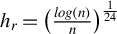
$h_r=\big (\frac {log(n)}{n} \big )^{\frac {1}{24}}$
 ,
$h_Y=\big (\frac {log(n)}{n} \big )^{\frac {1}{3}}$
 ,
$h_\epsilon =\big (\frac {log(n)}{n} \big )^{\frac {1}{4}}$
 , and
$h_{fr}=\big (\frac {log(n)}{n} \big )^{\frac {2}{7}}$
 . It is straightforward to verify that all conditions required for Theorem 3 are satisfied. Under these parameters, the convergence rate is
$O_p\Big ( \big (\frac {log(n)}{n} \big )^{\frac {1}{21}} \Big )$
 .
3.2 Fixed Effects Model
3.2.1 Estimator
First, we use the NW kernel estimator to estimate
$f_2(x_2,\mathbf {z}_2)$
 as follows:

where
$K_{i,h_{fd}}(x_2,\mathbf {z}_2,\bar {x}_3,\bar {\mathbf {z}}_3)=\frac {1}{h_{fd}^{2p+2}}\times k(\frac {X_{i2}-x_2}{h_{fd}}) \times k(\frac {Z_{i2,1}-z_{2,1}}{h_{fd}})\times \dots \times k(\frac {Z_{i2,p}-z_{2,p}}{h_{fd}})\times k(\frac {X_{i3}-\bar {x}_3}{h_{fd}}) \times k(\frac {Z_{i3,1}-\bar {z}_{3,1}}{h_{fd}})\times \dots \times k(\frac {Z_{i3,p}-\bar {z}_{3,p}}{h_{fd}})$
 . In this expression,
$k(\cdot )$
 denotes a univariate kernel function, and
$h_{fd}$
 is the bandwidth (Li and Racine, Reference Li and Racine2007, Chap. 2). We estimate
$f_3(x_3,\mathbf {z}_3)$
 using an analogous NW construction.
Next, following Equation (B.5), we estimate the conditional CDF of
$f_1(X_{i1},\mathbf {Z}_{i1})$
 as follows:

where
$\phi _f(\cdot )$
 is the Fourier transform of a kernel function
$K_f(\cdot )$
 with bounded support, and
$h_{f}$
 is a bandwidth parameter converging to zero (Fan, Reference Fan1991b; Evdokimov, Reference Evdokimov2010). We estimate
$\phi _{Y_{i1}-Y_{i2}+f_2(X_{i2},\mathbf {Z}_{i2})}(s|\mathbf {Z}_{i1}=\mathbf {z}_1)$
 in Equation (6) as follows:

where
$K_{i,h_{Y_d}}(\mathbf {z}_1)=\frac {1}{h_{Yd}^{p}} k(\frac {Z_{i1,1}-z_{1,1}}{h_{Yd}})\times \dots \times k(\frac {Z_{i1,p}-z_{1,p}}{h_{Yd}})$
 with bandwidth
$h_{Yd}$
 , and
$\hat {f}_2(X_{i2},\mathbf {Z}_{i2})$
 follows Equation (5). By identification, we have
$\phi _{\eta _{i1}-\eta _{i2}}(s|\mathbf {Z}_{i1}=\mathbf {z}_1)=\phi _{\eta _{i1}-\eta _{i2}}(s)=\phi _{\eta _{i3}-\eta _{i2}}(s)=\phi _{\eta _{i3}-\eta _{i2}}(s|X_{i3}=\bar {x}_3,\mathbf {Z}_{i3}=\bar {\mathbf {z}}_3)$
 . Therefore,
$\phi _{\eta _{i1}-\eta _{i2}}(s|\mathbf {Z}_{i1}=\mathbf {z}_1)$
 (equivalently,
$\phi _{\eta _{i1}-\eta _{i2}}(s)$
 ) in Equation (6) can be estimated as follows:

where
$K_{i,h_{\epsilon d}}(\bar {x}_3, \bar {\mathbf {z}}_3)=\frac {1}{h_{\epsilon d}^{p+1}}\times k(\frac {X_{i3}-\bar {x}_3}{h_{\epsilon d}}) \times k(\frac {Z_{i3,1}-\bar {z}_{3,1}}{h_{\epsilon d}})\times \dots \times k(\frac {Z_{i3,p}-\bar {z}_{3,p}}{h_{\epsilon d}})$
 with bandwidth
$h_{\epsilon d}$
 , and
$\hat {f}_2(X_{i2},\mathbf {Z}_{i2})$
 follows Equation (5). The rearrangement technique of Chernozhukov, Fernández-Val, and Galichon (Reference Chernozhukov, Fernández-Val and Galichon2010) can be applied to ensure that the estimated conditional CDF of
$f_1(X_{i1},\mathbf {Z}_{i1})$
 is strictly increasing.
Then, we estimate
$f_1(x_1,\mathbf {z}_1)$
 as follows:

where the conditional CDF
$F_{f_1(X_{i1},\mathbf {Z}_{i1})}(.|\mathbf {Z}_{i1}=\bar {\mathbf {z}}_1)$
 is estimated via Equation (6), and the conditional quantile
$F^{-1}_{f_1(X_{i1},\mathbf {Z}_{i1})}(.|\mathbf {Z}_{i1}=\mathbf {z}_1)$
 is obtained by inverting the corresponding estimated conditional CDF. As usual, the point
$(x_1,\mathbf {z}_1)$
 should be taken from the interior. Additionally, we construct estimators for the functionals of
$f_t(\cdot )$
 using a procedure analogous to that in the random effects model.
3.2.2 Convergence Rate
The convergence rates (and other asymptotic properties) of
$\hat {f}_2(x_2,\mathbf {z}_2)$
 and
$\hat {f}_3(x_3,\mathbf {z}_3)$
 are well established and therefore omitted. Under Assumptions CFE1–CFE7 in Appendix A.2, and defining
$\chi _d(h_f^{-1})=\max _t \sup _{s \in [-h_f^{-1},h_{f}^{-1}]} \frac {1}{|\phi _{\eta _{it}-\eta _{i,t+1}}(s)|}$
 , we establish the convergence rate of
$\hat {f}_1(x_1,\mathbf {z}_1)$
 .
Theorem 4. Suppose Assumptions FE1–FE4 and CFE1–CFE7 are satisfied. Further, for some small
$\delta>0$
 , assume that
$f_{X_{i1}}(x_1)$
 and
$\frac {\partial f_1(x_1,\mathbf {z}_1)}{\partial x_1}$
 are bounded away from zero and infinity for all
$x_1 \in [Q_{X_{i1}}(\delta /2),Q_{X_{i1}}(1-\delta /2)]$
 and
$\mathbf {z}_1 \in \mathcal {Z}_1$
 . Then,

There are two primary differences between Theorems 3 and 4. First, since
$f_2(x_2,\mathbf {z}_2)$
 is estimated using
$\hat {\mathbf {E}}[Y_{i2}|X_{i2},\mathbf {Z}_{i2}]$
 in the random effects model but via
$\hat {\mathbf {E}}[Y_{i2}-Y_{i3}|X_{i2},\mathbf {Z}_{i2},X_{i3},\mathbf {Z}_{i3}]$
 in the fixed effects model, Theorem 3 includes the term
$[log(n)/nh_{fr}^{p+1}]^{1/2}+(p+1)h_{fr}^{\bar {k}}$
 , whereas Theorem 4 includes
$[log(n)/nh_{fd}^{2p+2}]^{1/2} +(2p+2)h_{fd}^{\bar {k}}$
 . Second, the term
$[log(n)/nh_{fd}^{2p+2}]^{1/2}+(2p+2)h_{fd}^{\bar {k}}$
 appears in the second part of the expression in Theorem 4 but is absent from Theorem 3. This difference arises because the numerator of the estimator for
$\phi _{f_1(X_{i1}, \mathbf {Z}_{i1})}(s|\mathbf {Z}_{i1}=\mathbf {z}_1)$
 in the fixed effects model requires a first-stage estimation of
$f_2(X_{i2},\mathbf {Z}_{i2})$
 , whereas that in the random effects model does not. Aside from these two differences, the remaining components of Theorem 4 closely resemble those of Theorem 3. The full proof is provided in Appendix B.
The following example illustrates Theorem 4. Suppose
$p=1$
 ,
$\bar {k}=2$
 ,
$k_F=2$
 , and
$\gamma =5$
 . Let
$\eta _{i1}$
 ,
$\eta _{i2}$
 , and
$\eta _{i3}$
 be independent and follow
$Normal(0,1/2)$
 distributions (i.e., super-smooth), yielding
$\chi _d(h_{f}^{-1})=\exp ((h_{f}^{-1})^2/2)$
 . Set the bandwidths as
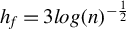
$h_f=3log(n)^{-\frac {1}{2}}$
 ,
$h_{Yd}=\big (\frac {log(n)}{n} \big )^{\frac {1}{3}}$
 ,
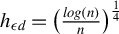
$h_{\epsilon d}=\big (\frac {log(n)}{n} \big )^{\frac {1}{4}}$
 , and
$h_{fd}=\big (\frac {log(n)}{n} \big )^{\frac {1}{8}}$
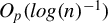
 . It is straightforward to verify that all conditions required for Theorem 4 are satisfied. Under these parameters, the convergence rate is
$O_p (log(n)^{-1} )$
 .
4 SIMULATION
In this section, we conduct two simulations to study the small-sample properties of
$\hat {f}_1(x_{1},\mathbf {z}_{1})$
 . The first considers the random effects model, and the second examines the fixed effects model.
4.1 Simulation I: Random Effects Model
We consider the following specification:


The functional form for
$f_1(X_{i1}, Z_{i1})$
 follows Evdokimov (Reference Evdokimov2010), while the specification for
$f_2(X_{i2}, Z_{i2})$
 is motivated by our empirical exercise.Footnote
5
The variables
$X_{it}$
 and
$Z_{it}$
 are drawn from
$Uniform(0,1)$
 distributions, and
$\alpha _i$
 follows a standard normal distribution. We assume that
$\eta _{i1}$
 and
$\eta _{i2}$
 are standard normal (super-smooth). The independence between the persistent heterogeneity
$\alpha _i$
 and the regressors
$(X_{it},Z_{it})$
 characterizes this as a random effects model.
We run 500 repetitions with sample sizes of 2,500, 5,000, and 10,000 observations. In each repetition, we estimate
$f_1(x_1,z_1)$
 at 200 fixed points
$(x_1,z_1)$
 drawn from the 10th to 90th percentiles of their distributions. We use the NW kernel estimator from Section 3 and the LL kernel estimator, the latter of which is less sensitive to boundary bias. Following Evdokimov (Reference Evdokimov2010), we consider two bandwidth settings for deconvolution. First is
$h_\epsilon =h_{fr}=h_r=0.4$
 , followed by
$h_\epsilon =h_{fr}=h_r=0.6$
 .Footnote
6
We also include an “infeasible” benchmark, where
$f_1(x_1,z_1)$
 is estimated using the NW kernel under full observability of
$X_{i1}$
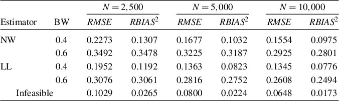
 . Table 1 reports the root mean squared error (
$RMSE$
 ) and root mean squared bias (
$RBIAS^2$
 ), defined as follows:


Random effects model with
$X_{i1}$
 completely missing

Table 1 Long description
The table is organized into columns for Estimator, B W, and three main groups based on sample size N.
* Header Row 1: Sample sizes N equals 2,500, N equals 5,000, and N equals 10,000.
* Header Row 2: Under each N value, there are sub-columns for R M S E and R B I A S squared.
Data Rows:
* N W Estimator:
- At B W 0.4: R M S E ranges from 0.2273 to 0.1554; R B I A S squared ranges from 0.1307 to 0.0975 as N increases.
- At B W 0.6: R M S E ranges from 0.3492 to 0.2925; R B I A S squared ranges from 0.3478 to 0.2801 as N increases.
* L L Estimator:
- At B W 0.4: R M S E ranges from 0.1952 to 0.1345; R B I A S squared ranges from 0.1192 to 0.0776 as N increases.
- At B W 0.6: R M S E ranges from 0.3076 to 0.2608; R B I A S squared ranges from 0.3061 to 0.2494 as N increases.
* Infeasible Estimator:
- R M S E ranges from 0.1029 to 0.0648; R B I A S squared ranges from 0.0265 to 0.0173 as N increases.
4.2 Simulation II: Fixed Effects Model
We consider the following specification:


The functional forms for
$f_1(\cdot )$
 and
$f_2(\cdot )$
 are identical to those in the random effects model, and the specification for
$f_3(\cdot )$
 follows Evdokimov (Reference Evdokimov2010). The variables
$X_{it}$
 and
$Z_{it}$
 are drawn from
$Uniform(0,1)$
 distributions, and the unobserved persistent heterogeneity is defined as
$\alpha _i=0.5\sum _{t=1}^3(X_{it}-0.5)+0.5\ Normal(0,1)$
 . We assume that
$\eta _{i1}$
 ,
$\eta _{i2}$
 , and
$\eta _{i3}$
 follow standard normal distributions. Because the unobserved persistent heterogeneity is correlated with the regressors, this constitutes a fixed effects model.
Consistent with the previous simulation, we run 500 repetitions with sample sizes of 2,500, 5,000, and 10,000 observations. In each repetition, we estimate
$f_1(x_1,z_1)$
 at 200 fixed points
$(x_1,z_1)$
 drawn from the 10th to 90th percentiles of their distributions. We use the NW and LL kernel estimators and consider two bandwidth settings for deconvolution:
$0.4$
 and
$0.6$
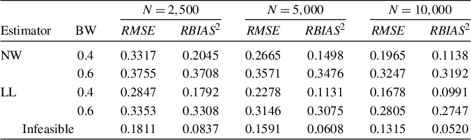
 . We also include an “infeasible” benchmark estimator. Table 2 reports the
$RMSE$
 and
$RBIAS^2$
 , defined previously.
Fixed effects model with
$X_{i1}$
 completely missing

Table 2 Long description
A table with eight columns. The first column is Estimator, the second is B W, and the remaining six columns are grouped under three sample sizes: N = 2,500, N = 5,000, and N = 10,000. Each sample size has two sub-columns: R M S E and R B I A S squared.
* Row 1: Estimator N W, B W 0.4. N = 2,500: R M S E 0.3317, R B I A S squared 0.2045. N = 5,000: R M S E 0.2665, R B I A S squared 0.1498. N = 10,000: R M S E 0.1965, R B I A S squared 0.1138.
* Row 2: Estimator N W, B W 0.6. N = 2,500: R M S E 0.3755, R B I A S squared 0.3708. N = 5,000: R M S E 0.3571, R B I A S squared 0.3476. N = 10,000: R M S E 0.3247, R B I A S squared 0.3192.
* Row 3: Estimator L L, B W 0.4. N = 2,500: R M S E 0.2847, R B I A S squared 0.1792. N = 5,000: R M S E 0.2278, R B I A S squared 0.1131. N = 10,000: R M S E 0.1678, R B I A S squared 0.0991.
* Row 4: Estimator L L, B W 0.6. N = 2,500: R M S E 0.3353, R B I A S squared 0.3308. N = 5,000: R M S E 0.3146, R B I A S squared 0.3075. N = 10,000: R M S E 0.2805, R B I A S squared 0.2747.
* Row 5: Estimator Infeasible. N = 2,500: R M S E 0.1811, R B I A S squared 0.0837. N = 5,000: R M S E 0.1591, R B I A S squared 0.0608. N = 10,000: R M S E 0.1315, R B I A S squared 0.0520.
The simulation results show that the estimators perform well in small samples. Several additional patterns emerge. First, a bandwidth of 0.4 outperforms 0.6 in both models, yielding smaller and more balanced
$RMSE$
 and
$RBIAS^2$
 values, consistent with the conditional deconvolution literature. Second, performance improves with sample size. Third, the NW and LL kernel estimators produce similar results, as the evaluation points exclude boundary regions. Finally, Simulation I exhibits better results than Simulation II because the latter applies first-differencing to eliminate unobserved persistent heterogeneity, introducing additional conditioning variables; this result is consistent with Theorems 3 and 4.
5 EMPIRICAL EXERCISE
Understanding the mechanisms underlying mathematical difficulties is essential for developing competencies required for academic and professional success (Peng and Lin, Reference Peng and Lin2019; Lin, Peng, and Luo, Reference Lin, Peng and Luo2021). In this section, we examine the effect of MV on computation (COM) among fourth- and sixth-grade Chinese elementary students. Section 5.1 describes the data, and Section 5.2 presents the estimation results.
5.1 Data
We use a dataset from Lin, Peng, and Luo (Reference Lin, Peng and Luo2021) comprising 237 participants (125 boys) from a representative elementary school in southern China. The school was selected because, according to county education bureau records, its academic performance aligns with the county average. MV is measured using multiple-choice questions covering the relevant vocabulary for fourth and sixth grades, where students select either the correct definition of a term or the term corresponding to a given definition. COM is assessed using the Wide Range Achievement Test, in which students have 30 minutes to complete 80 calculation problems of increasing difficulty. For this test, a small number of English terms were translated into Chinese. Scores are defined as the number of correctly solved items.
Computation data are available for both the fourth and sixth grades. However, MV data were collected only for the fourth grade, leaving sixth-grade observations completely missing due to funding and time constraints.Footnote
7
The regressors
$\mathbf {Z}_{it}$
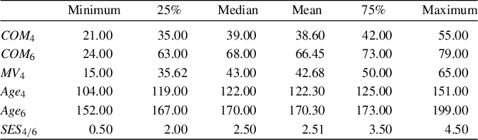
 include age (measured in months) and SES, both of which are fully observed for both grades. Table 3 reports the summary statistics.
Summary statistics of data

Table 3 Long description
The table consists of seven columns and six data rows. The columns are labeled: Variable (unlabeled in header), Minimum, 25%, Median, Mean, 75%, and Maximum.
* Row 1: COM sub 4. Minimum 21.00, 25% 35.00, Median 39.00, Mean 38.60, 75% 42.00, Maximum 55.00.
* Row 2: COM sub 6. Minimum 24.00, 25% 63.00, Median 68.00, Mean 66.45, 75% 73.00, Maximum 79.00.
* Row 3: M V sub 4. Minimum 15.00, 25% 35.62, Median 43.00, Mean 42.68, 75% 50.00, Maximum 65.00.
* Row 4: Age sub 4. Minimum 104.00, 25% 119.00, Median 122.00, Mean 122.30, 75% 125.00, Maximum 151.00.
* Row 5: Age sub 6. Minimum 152.00, 25% 167.00, Median 170.00, Mean 170.30, 75% 173.00, Maximum 199.00.
* Row 6: S E S sub 4 forward slash 6. Minimum 0.50, 25% 2.00, Median 2.50, Mean 2.51, 75% 3.50, Maximum 4.50.
5.2 Estimation Results
We employ the following nonparametric random effects panel data modelFootnote 8 :

Applying the identification and estimation strategies developed in this article, we examine the average marginal effects of MV on COM, defined as
$\mathbf {E}[\frac {\partial f_t(MV_{it},\mathbf {Z}_{it})}{\partial mv}]$
 for
$t \in \{4, 6\}$
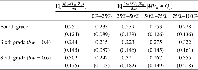
 . For the sixth-grade sample, we set the deconvolution bandwidths to 0.4 and 0.6 to maintain consistency with the simulations. The first column of Table 4 reports the results. For fourth-grade students, the estimated effect is 0.251 (s.e. 0.124). For sixth-grade students, the estimates exhibit some sensitivity to bandwidth choice: the estimate closest to the fourth-grade result is 0.244 (s.e. 0.145), obtained with a bandwidth of 0.4.Footnote
9
These findings highlight the important role of MV in developing computational proficiency.
Effects of MV on COM in different grades

Table 4 Long description
The table consists of six columns. The first column lists the grade levels: Fourth grade, Sixth grade with bw equal to 0.4, and Sixth grade with bw equal to 0.6.
Column 2 is labeled with the expectation of the partial derivative of f sub t with respect to m v. The values are:
- Fourth grade: 0.251 (standard error 0.124).
- Sixth grade (0.4): 0.244 (standard error 0.145).
- Sixth grade (0.6): 0.302 (standard error 0.175).
Columns 3 through 6 represent quartiles (0% to 25%, 25% to 50%, 50% to 75%, and 75% to 100%) for the conditional expectation of the partial derivative given M V sub i t is in Q sub j.
For Fourth grade:
- 0% to 25%: 0.233 (0.089)
- 25% to 50%: 0.239 (0.139)
- 50% to 75%: 0.253 (0.126)
- 75% to 100%: 0.278 (0.136)
For Sixth grade (bw = 0.4):
- 0% to 25%: 0.215 (0.087)
- 25% to 50%: 0.223 (0.146)
- 50% to 75%: 0.275 (0.145)
- 75% to 100%: 0.322 (0.161)
For Sixth grade (bw = 0.6):
- 0% to 25%: 0.242 (0.103)
- 25% to 50%: 0.321 (0.182)
- 50% to 75%: 0.267 (0.149)
- 75% to 100%: 0.355 (0.218)
Note: Standard errors are reported in parentheses.
Compared with linear models, the nonparametric approach offers the advantage of capturing more complex effects of MV on COM. We partition the support of MV into empirical quartiles,
$\mathcal {Q}_j$
 , defined by the intervals
$[F_{MV_{it}}^{-1}(\frac {j-1}{4}), F_{MV_{it}}^{-1}(\frac {j}{4})]$
 for
$j=1, \dots , 4$
 . We then estimate the average marginal effects within each segment:
$\mathbf {E} \left [ \frac {\partial f_t(MV_{it},\mathbf {Z}_{it})}{\partial mv} | MV_{it} \in \mathcal {Q}_j \right ]$
 . Columns 2–5 of Table 4 show that these effects vary with the level of MV. For both fourth- and sixth-grade students, the marginal effects increase with MV, indicating that MV has a progressively stronger impact on computational performance.
6 CONCLUSION
The nonparametric time-varying panel data model has gained considerable attention in recent years. However, identification and estimation become challenging when primary regressors are completely missing in some time periods due to funding constraints, time limitations, storage capacity, or legal requirements. This article proposes a novel strategy to address these challenges. Under standard assumptions from the panel data and nonparametric literature, we establish the identification of the unknown functions and the distributions of the missing regressors. Specifically, the random effects model is identified with one period of completely observed data, whereas the fixed effects model requires two. Following identification, we construct estimators: in periods with fully observed data, estimation relies on conditional expectations; in periods with missing data, it combines conditional CDFs and quantiles. We derive uniform convergence rates for these estimators and demonstrate favorable small-sample performance through simulation studies. An empirical application examining the effect of MV on computation further illustrates the relevance and applicability of the proposed method.
APPENDIX
A ASSUMPTIONS FOR CONVERGENCE RATES
A.1 Random Effects Model Assumptions
We impose smoothness and regularity assumptions on the random variables and the unknown functions (Fan, Reference Fan1991b; Evdokimov, Reference Evdokimov2010). A function
$\psi : \mathbf {S} \times \mathbf {W} \rightarrow \, \mathbb {C}$
 , where
$\mathbf {S} \subset \mathbb {R}$
 and
$\mathbf {W} \subset \mathbb {R}^p$
 , is said to belong to the class of functions
$\mathbf {D}_{\mathbf {W}}^{\mathbf {S}}(k)$
 if it is
$k$
 times continuously differentiable in
$w$
 , and there is a constant
$A>0$
 such that
$\sup _{w \in \mathbf {W}} \max _{|\alpha |=l} |\partial ^{\alpha }_{w} \psi (s,w)| \leq A(1+|s|^l)$
 for all
$l\leq k$
 and all
$s$
 on the support. Here,
$\partial ^{\alpha }_{w} \psi (s,w)$
 is defined as
$\partial ^{|\alpha |} \psi (s,w) / \partial w_1^{\alpha _1} \dots \partial w_p^{\alpha _p}$
 with
$|\alpha | = \alpha _1 + \dots + \alpha _p$
 .
Assumption CRE1.
$F_{f_1(X_{i1},\mathbf {Z}_{i1})}(f_1(x_1,\mathbf {z}_1)|\mathbf {Z}_{i1}=\mathbf {z}_1)$
 has
$k_F$
 continuous absolutely integrable derivatives for all
$f_1(x_1,\mathbf {z}_1)$
 and
$\mathbf {z}_1$
 on the support.
Assumption CRE2. For
$t \in \{1,2\}$
 : (i) the support of
$(X_{it},\mathbf {Z}_{it})$
 is bounded; (ii)
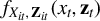
$f_{X_{it},\mathbf {Z}_{it}}(x_t,\mathbf {z}_t)$
 is bounded from above and away from zero for all
$(x_t,\mathbf {z}_t)$
 on the support; and (iii) there is a positive integer
$\bar {k} \geq 1$
 such that
$f_{X_{it},\mathbf {Z}_{it}}(x_t,\mathbf {z}_t)$
 has
$\bar {k}$
 continuous mixed partial derivatives.
Assumption CRE3. For
$t \in \{1,2\}$
 : (i) there is a constant
$\gamma>2$
 such that
$\sup _{x_t,\mathbf {z}_t} \mathbf {E}[|Y_{it}|^\gamma |X_{it}=x_t,\mathbf {Z}_{it}=\mathbf {z}_t]$
 is bounded and (ii)
$\mathbf {E}[Y_{it}|X_{it}=x_t,\mathbf {Z}_{it}=\mathbf {z}_t]$
 is
$\bar {k}$
 -th differentiable.
Assumption CRE4.
$\phi _{f_1(X_{i1},\mathbf {Z}_{i1})}(s|\mathbf {Z}_{i1}=\mathbf {z}_1) \in \mathbf {D}_{\mathcal {Z}_1}^{[-h_r^{-1},h_{r}^{-1}]}(\bar {k})$
 ,
$\partial \phi _{f_1(X_{i1},\mathbf {Z}_{i1})}(s|\mathbf {Z}_{i1}=\mathbf {z}_1)/\partial s \in \mathbf {D}_{\mathcal {Z}_1}^{[-h_r^{-1},h_{r}^{-1}]}(\bar {k})$
 .
Assumption CRE1 is stronger than the conventional assumption of bounded derivatives and is needed to establish the convergence rate of the Fourier regularization bias. Assumptions CRE2 and CRE3 are standard conditions on the support, the smoothness of the density and the regression function, and the conditional moment of the outcome variable for deriving uniform convergence rate. Assumption CRE4 imposes smoothness conditions on
$\phi _{f_1(X_{i1},\mathbf {Z}_{i1})}(s|\mathbf {Z}_{i1}=\mathbf {z}_1)$
 and its first derivative. These conditions are required to establish the uniform convergence rate of the weighted characteristic function estimation error appearing in the deconvolution step.
The tail behavior of the characteristic function of
$\epsilon _{it}$
 is critical in determining the difficulty of deconvolution. As discussed in Fan (Reference Fan1991b), a smoother distribution of
$\epsilon _{it}$
 leads to a more challenging deconvolution. Two categories are typically considered: ordinary-smooth (e.g., Gamma and Laplace) and super-smooth (e.g., Normal and Cauchy). In our simulations, we consider that
$\epsilon _{it}$
 follows a normal distribution. Recalling the notation introduced in the main text, we write

The next three assumptions are on the kernel functions and bandwidths used in estimation (Fan, Reference Fan1991b; Evdokimov, Reference Evdokimov2010).
Assumption CRE5. The Fourier transform
$\phi _r(\cdot )$
 is continuously differentiable, has support [-1,1], and satisfies
$\phi _r(s)=1+O(|s|^{k_F})$
 as
$s \rightarrow 0$
 .
Assumption CRE6.
$k(\cdot )$
 is a bounded, integrable, univariate
$\bar {k}$
 -th-order kernel function.
Assumption CRE7.
-
(i) $h_Y \rightarrow 0$
,
$nh_Y \rightarrow \infty $
,
$h_\epsilon \rightarrow 0$
,
$nh_\epsilon \rightarrow \infty $
,
$h_{fr} \rightarrow 0$
,
$nh_{fr} \rightarrow \infty $
,
$h_r \rightarrow 0$
. -
(ii) $(log(n))^{1/2} n^{1/\gamma -1/2}h_Y^{-p/2} \rightarrow 0 $
,
$(log(n))^{1/2} n^{1/\gamma -1/2}h_\epsilon ^{-(p+1)/2} \rightarrow 0 $
. -
(iii) $(log(n))^{\gamma -3/2}h_r^{-1}h_Y^{p/2}n^{1/\gamma -1/2} \rightarrow 0$
,
$(log(n))^{\gamma -3/2}h_r^{-1}h_\epsilon ^{(p+1)/2}n^{1/\gamma -1/2} \rightarrow 0$
. -
(iv) $h_r^{-1}\big ([log(n)/nh_\epsilon ^{p+1}]^{1/2}+h_r^{-(\bar {k}-1)}h_\epsilon ^{\bar {k}}+ [log(n)/nh_{fr}^{p+1}]^{1/2}+(p+1)h_{fr}^{\bar {k}} \big ) \chi ^2(h_r^{-1}) \rightarrow 0$
.







Assumption CRE5 concerns the Fourier regularization function, and Assumption CRE6 specifies the univariate kernel function used in estimation; both are standard conditions. Assumptions CRE7(i) and (iv) are needed for consistency. In particular, Assumption CRE7(iv) ensures that
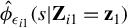
$\sup _{(s,\mathbf {z}_1)\in [-1/h_r,1/h_r]\times \bar {\mathcal {Z}}_1}\Big | \frac {\hat {\phi }_{\epsilon _{i1}}(s|\mathbf {Z}_{i1}=\mathbf {z}_1)-\phi _{\epsilon _{i1}}(s|\mathbf {Z}_{i1}=\mathbf {z}_1)}{\phi _{\epsilon _{i1}}(s|\mathbf {Z}_{i1}=\mathbf {z}_1)} \Big |=o_p(1)$
 , which is necessary because
${\hat {\phi }_{\epsilon _{i1}}(s|\mathbf {Z}_{i1}=\mathbf {z}_1)}$
 appears in the denominator of the estimator
$\hat {F}_{f_1(X_{i1},\mathbf {Z}_{i1})}(f_1(x_1,\mathbf {z}_1)|\mathbf {Z}_{i1}=\mathbf {z}_1)$
 . Assumptions CRE7(ii) and (iii) require the tails of
$Y_{it}$
 to be sufficiently thin. Although these conditions are not necessary for consistency, they simplify the expression for the uniform convergence rate.
A.2 Fixed Effects Model Assumptions
The following assumptions are needed to derive the convergence rates of the fixed effects model. Recall that
$\chi _d(h_f^{-1})$
 is defined as
$\max _t \sup _{s \in [-h_f^{-1},h_{f}^{-1}]} \frac {1}{|\phi _{\eta _{it}-\eta _{i,t+1}}(s)|}$
 .
Assumption CFE1.
$F_{f_1(X_{i1},\mathbf {Z}_{i1})}(f_1(x_1,\mathbf {z}_1)|\mathbf {Z}_{i1}=\mathbf {z}_1)$
 has
$k_F$
 continuous absolutely integrable derivatives for all
$f_1(x_1,\mathbf {z}_1)$
 and
$\mathbf {z}_1$
 on the support.
Assumption CFE2. For
$t \in \{1,2,3\}$
 : (i) the support of
$(X_{it},\mathbf {Z}_{it})$
 is bounded; (ii)
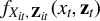
$f_{X_{it},\mathbf {Z}_{it}}(x_t,\mathbf {z}_t)$
 is bounded from above and away from zero for all
$(x_t,\mathbf {z}_t)$
 on the support; and (iii) there is a positive integer
$\bar {k} \geq 1$
 such that
$f_{X_{it},\mathbf {Z}_{it}}(x_t,\mathbf {z}_t)$
 has
$\bar {k}$
 continuous mixed partial derivatives.
Assumption CFE3. (i) There is a constant
$\gamma>2$
 such that
$\sup _{x_1,x_2,\mathbf {z}_1,\mathbf {z}_2} \mathbf {E}[|Y_{i1}-Y_{i2}|^\gamma |X_{i1}=x_1,X_{i2}=x_2,\mathbf {Z}_{i1}=\mathbf {z}_1,\mathbf {Z}_{i2}=\mathbf {z}_2]$
 and
$\sup _{x_2,x_3,\mathbf {z}_2,\mathbf {z}_3} \mathbf {E}[|Y_{i3}-Y_{i2}|^\gamma |X_{i2}=x_2,X_{i3}=x_3,\mathbf {Z}_{i2}=\mathbf {z}_2,\mathbf {Z}_{i3}=\mathbf {z}_3]$
 are bounded. (ii)
$\mathbf {E}[Y_{i3}-Y_{i2}|X_{i2}=x_2,\mathbf {Z}_{i2}=\mathbf {z}_2,X_{i3}=x_3,\mathbf {Z}_{i3}=\mathbf {z}_3]$
 is
$\bar {k}$
 -th differentiable.
Assumption CFE4.
$\phi _{f_1(X_{i1},\mathbf {Z}_{i1})}(s|\mathbf {Z}_{i1}=\mathbf {z}_1) \in \mathbf {D}_{\mathcal {Z}_1}^{[-h_f^{-1},h_{f}^{-1}]}(\bar {k})$
 ,
$\partial \phi _{f_1(X_{i1},\mathbf {Z}_{i1})}(s|\mathbf {Z}_{i1}=\mathbf {z}_1)/\partial s \in \mathbf {D}_{\mathcal {Z}_1}^{[-h_f^{-1},h_{f}^{-1}]}(\bar {k})$
 .
Assumption CFE5. The Fourier transform
$\phi _f(\cdot )$
 is continuously differentiable, has support [-1,1], and satisfies
$\phi _f(s)=1+O(|s|^{k_F})$
 as
$s \rightarrow 0$
 .
Assumption CFE6.
$k(\cdot )$
 is a bounded, integrable, univariate
$\bar {k}$
 -th-order kernel function.
Assumption CFE7.
-
(i) $h_{Yd} \rightarrow 0$
,
$nh_{Yd} \rightarrow \infty $
,
$h_{\epsilon d} \rightarrow 0$
,
$nh_{\epsilon d} \rightarrow \infty $
,
$h_{fd} \rightarrow 0$
,
$nh_{fd} \rightarrow \infty $
,
$h_{f} \rightarrow 0$
. -
(ii) $(log(n))^{1/2} n^{1/\gamma -1/2}h_{Yd}^{-p/2} \rightarrow 0 $
,
$(log(n))^{1/2} n^{1/\gamma -1/2}h_{\epsilon d}^{-(p+1)/2} \rightarrow 0 $
. -
(iii) $(log(n))^{\gamma -3/2}h_f^{-1}h_{Yd}^{p/2}n^{1/\gamma -1/2} \rightarrow 0$
,
$(log(n))^{\gamma -3/2}h_f^{-1}h_{\epsilon d}^{(p+1)/2}n^{1/\gamma -1/2} \rightarrow 0$
. -
(iv) $h_f^{-1}\big ([log(n)/nh_{\epsilon d}^{p+1}]^{1/2}+h_f^{-(\bar {k}-1)}h_{\epsilon d}^{\bar {k}}+ [log(n)/nh_{fd}^{2p+2}]^{1/2}+(2p+2)h_{fd}^{\bar {k}} \big ) \chi _d^2(h_f^{-1}) \rightarrow 0$
.






Assumption CFE2 extends Assumption CRE2 from two to three time periods, as required for the identification of the fixed effects model. Assumption CFE3 generalizes the conditional moment condition in Assumption CRE3 from single-period outcomes to first-differenced outcomes. The bandwidth conditions in Assumption CFE7 are modified to accommodate the additional conditioning variables arising from first differencing. Assumptions CFE1 and CFE4–CFE6 are analogous to those for the random effects model, differing only in notation.
B PROOFS
B.1 Proof of Theorem 1
Proof. Under Assumption RE1, the conditional expectation
$\mathbf {E}[Y_{i2}|X_{i2}=x_2,\mathbf {Z}_{i2}=\mathbf {z}_2]$
 identifies
$f_2(x_2,\mathbf {z}_2)$
 . We address the identification of
$f_1(x_1,\mathbf {z}_1)$
 by first recovering the characteristic function of
$\epsilon _{i1}$
 , denoted by
$\phi _{\epsilon _{i1}}(s)$
 . Under Assumptions RE1, RE2, and RE4, we have

Next, we identify the characteristic function of
$f_1(X_{i1},\mathbf {Z}_{i1})$
 conditional on
$\mathbf {Z}_{i1}=\mathbf {z}_1$
 for any
$\mathbf {z}_1$
 on the support. By Assumptions RE1 and RE4, we obtain

The numerator is identified from the data, and the denominator is identified by Equation (B.1), noting that
$\phi _{\epsilon _{i1}}(s|\mathbf {Z}_{i1}=\mathbf {z}_1)=\phi _{\epsilon _{i1}}(s)$
 . This conditional characteristic function identifies the conditional CDF as follows:

Finally, we identify
$f_1(x_1,\mathbf {z}_1)$
 using the identified conditional CDF and Assumptions RE1 and RE3. Specifically, it follows that

This implies

where
$F^{-1}_{(\cdot )}(\cdot |\cdot )$
 denotes the conditional quantile function. These results, together with Assumption RE1, establish that the distribution of
$X_{i1}$
 is also identified.
B.2 Proof of Theorem 2
Proof. We employ first-differencing to eliminate the unobserved persistent heterogeneity
$\alpha _i$
 :


Under Assumptions FE1–FE3,
$\mathbf {E}[Y_{i2}-Y_{i3}|X_{i2}=x_2,\mathbf {Z}_{i2}=\mathbf {z}_2,X_{i3}=\bar {x}_3,\mathbf {Z}_{i3}=\bar {\mathbf {z}}_3]$
 identifies
$f_2(x_2,\mathbf {z}_2)$
 . This, in turn, allows
$\mathbf {E}[Y_{i3}-Y_{i2}+f_2(X_{i2},\mathbf {Z}_{i2})|X_{i3}=x_3,\mathbf {Z}_{i3}=\mathbf {z}_3]$
 to identify
$f_3(x_3,\mathbf {z}_3)$
 .
We identify
$f_1(x_1, \mathbf {z}_1)$
 by first recovering the characteristic function of
$\eta _{i1}-\eta _{i2}$
 , denoted by
$\phi _{\eta _{i1}-\eta _{i2}}(s)$
 . Under Assumptions FE1–FE4, we have

Next, we identify the characteristic function of
$f_1(X_{i1}, \mathbf {Z}_{i1})$
 conditional on
$\mathbf {Z}_{i1}=\mathbf {z}_1$
 for any
$\mathbf {z}_1$
 on the support. By Assumptions FE1 and FE4, we obtain

The numerator is identified from the data and the previous step, and the denominator is identified by Equation (B.4) because
$\phi _{\eta _{i1}-\eta _{i2}}(s|\mathbf {Z}_{i1}=\mathbf {z}_1)=\phi _{\eta _{i1}-\eta _{i2}}(s)$
 . This conditional characteristic function identifies the conditional CDF as follows:

Finally, we identify
$f_1(x_1,\mathbf {z}_1)$
 using the identified conditional CDF and Assumptions FE1 and FE3:

where
$F^{-1}_{(\cdot )}(\cdot |\cdot )$
 denotes the conditional quantile function. These results, together with Assumption FE1, establish that the distribution of
$X_{i1}$
 is also identified.
B.3 Proof of Theorem 3
Proof. We first derive the convergence rate of
$\hat {F}_{f_1(X_{i1},\mathbf {Z}_{i1})}(f_1(x_1,\mathbf {z}_1)|\mathbf {Z}_{i1}=\mathbf {z}_1)$
 . By the definition of
$\hat {F}_{f_1(X_{i1},\mathbf {Z}_{i1})}(f_1(x_1,\mathbf {z}_1)|\mathbf {Z}_{i1}=\mathbf {z}_1)$
 , we have

This decomposition consists of two terms. The first term captures the Fourier regularization bias, while the second captures the estimation error arising from replacing
$\phi _{Y_{i1}}(s|\mathbf {Z}_{i1}=\mathbf {z}_1)$
 and
$\phi _{\epsilon _{i1}}(s|\mathbf {Z}_{i1}=\mathbf {z}_1)$
 with their estimators.
Under Assumptions CRE1 and CRE5, standard arguments from the conditional deconvolution literature, as in Evdokimov (Reference Evdokimov2010), show that the first term satisfies

We expand
$\frac {1}{s} \Big [ \frac {\hat {\phi }_{Y_{i1}}(s|\mathbf {Z}_{i1}=\mathbf {z}_1)}{\hat {\phi }_{\epsilon _{i1}}(s|\mathbf {Z}_{i1}=\mathbf {z}_1)}-\frac {\phi _{Y_{i1}}(s|\mathbf {Z}_{i1}=\mathbf {z}_1)}{\phi _{\epsilon _{i1}}(s|\mathbf {Z}_{i1}=\mathbf {z}_1)} \Big ]$
 appearing in the second term as

We define

Unlike
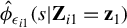
$\hat {\phi }_{\epsilon _{i1}}(s|\mathbf {Z}_{i1}=\mathbf {z}_1)$
 , which requires estimating
$f_2(X_{i2},\mathbf {Z}_{i2})$
 ,
$\tilde {\phi }_{\epsilon _{i1}}(s|\mathbf {Z}_{i1}=\mathbf {z}_1)$
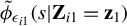 is the estimator that treats
$f_2(X_{i2},\mathbf {Z}_{i2})$
 as known.
Under Assumptions CRE1–CRE7, it follows from the uniform convergence rate for nonparametric regression (see, e.g., Li and Racine, Reference Li and Racine2007, Thm. 2.6) and the convergence results established by Evdokimov (Reference Evdokimov2010) for the conditional characteristic function estimator that

Then, the second term can be bounded as

Under Assumptions CRE1–CRE7, it follows from the convergence results established by Evdokimov (Reference Evdokimov2010) for the conditional characteristic function estimator that

Moreover, Assumption CRE1 implies that
$|\phi _{f_1(X_{i1},\mathbf {Z}_{i1})}(s|\mathbf {Z}_{i1}=\mathbf {z}_1)| <C$
 for
$|s| \leq 1$
 , and
$|\phi _{f_1(X_{i1},\mathbf {Z}_{i1})}(s|\mathbf {Z}_{i1}=\mathbf {z}_1)| <C|s|^{-(k_F-1)}$
 for
$|s|> 1$
 . Combining these decay properties with the preceding convergence result gives

Putting the bounds for the first and second terms together, the convergence rate of the conditional CDF is

Next, we derive the convergence rate of
$\hat {F}^{-1}_{f_1(X_{i1},\mathbf {Z}_{i1})}(q|\mathbf {Z}_{i1}=\mathbf {z}_1)$
 . Under Assumptions CRE1–CRE7, applying the convergence results for conditional quantile estimators established by Evdokimov (Reference Evdokimov2010), we obtain

The conclusion of Theorem 3 follows directly from Equations (B.7) and (B.8).
B.4 Proof of Theorem 4
Proof. We first derive the convergence rate of
$\hat {F}_{f_1(X_{i1},\mathbf {Z}_{i1})}(f_1(x_1,\mathbf {z}_1)|\mathbf {Z}_{i1}=\mathbf {z}_1)$
 . By the definition of
$\hat {F}_{f_1(X_{i1},\mathbf {Z}_{i1})}(f_1(x_1,\mathbf {z}_1)|\mathbf {Z}_{i1}=\mathbf {z}_1)$
 , we have

The first term captures the Fourier regularization bias, while the second captures the estimation error induced by replacing the conditional characteristic functions by their estimators.
Under Assumptions CFE1 and CFE5, standard arguments from the conditional deconvolution literature, as in Evdokimov (Reference Evdokimov2010), show that the first term satisfies

We expand
$\frac {1}{s} \Big [\frac {\hat {\phi }_{Y_{i1}-Y_{i2}+\hat {f}_2(X_{i2},\mathbf {Z}_{i2})}(s|\mathbf {Z}_{i1}=\mathbf {z}_{1})}{\hat {\phi }_{\eta _{i1}-\eta _{i2}}(s|\mathbf {Z}_{i1}=\mathbf {z}_{1})}-\frac {\phi _{Y_{i1}-Y_{i2}+f_2(X_{i2},\mathbf {Z}_{i2})}(s|\mathbf {Z}_{i1}=\mathbf {z}_{1})}{\phi _{\eta _{i1}-\eta _{i2}}(s|\mathbf {Z}_{i1}=\mathbf {z}_{1})} \Big ]$
 appearing in the second term as

We define

Unlike
$\hat {\phi }_{\eta _{i1}-\eta _{i2}}(s|\mathbf {Z}_{i1}=\mathbf {z}_1)$
 , which requires estimating
$f_2(X_{i2},\mathbf {Z}_{i2})$
 ,
$\tilde {\phi }_{\eta _{i1}-\eta _{i2}}(s|\mathbf {Z}_{i1}=\mathbf {z}_1)$
 is the estimator that treats
$f_2(X_{i2},\mathbf {Z}_{i2})$
 as known.
Under Assumptions CFE1–CFE7, it follows from the uniform convergence rate for nonparametric regression (see, e.g., Li and Racine, Reference Li and Racine2007, Thm. 2.6) and the convergence results established by Evdokimov (Reference Evdokimov2010) for the conditional characteristic function estimator that

Then, the second term can be bounded as

By the Lipschitz property of complex exponential and L’Hôpital’s rule, it holds that

This bound, together with the uniform convergence rate of
$\hat {\phi }_{Y_{i1}-Y_{i2}+f_2(X_{i2},\mathbf {Z}_{i2})}(s|\mathbf {Z}_{i1}=\mathbf {z}_1)$
 , yields


Moreover, Assumption CFE1 implies that
$|\phi _{f_1(X_{i1},\mathbf {Z}_{i1})}(s|\mathbf {Z}_{i1}=\mathbf {z}_1)| <C$
 for
$|s| \leq 1$
 , and
$|\phi _{f_1(X_{i1},\mathbf {Z}_{i1})}(s|\mathbf {Z}_{i1}=\mathbf {z}_1)| <C|s|^{-(k_F-1)}$
 for
$|s|> 1$
 . Combining these decay properties with the preceding convergence result gives

Putting the bounds for the first and second terms together, the convergence rate of the conditional CDF is

Next, we derive the convergence rate of
$\hat {F}^{-1}_{f_1(X_{i1},\mathbf {Z}_{i1})}(q|\mathbf {Z}_{i1}=\mathbf {z}_1)$
 . Under Assumptions CFE1–CFE7, applying the convergence results for conditional quantile estimators established by Evdokimov (Reference Evdokimov2010), we obtain

The conclusion of Theorem 4 follows directly from Equations (B.9) and (B.10).
FUNDING STATEMENT
The author declares that no specific funding has been received for this article.
COMPETING INTERESTS
The author declares that no competing interests exist.