1. Introduction
Turbulence is a highly complex, irregular flow phenomenon that occurs in liquids, gases and plasma, making it ubiquitous in both nature and engineering applications (Pope Reference Pope2001). Although the numerical integration of the Navier–Stokes (NS) equations is a crucial tool for studying the fundamental mechanisms of turbulent flows, even the most powerful foreseeable computers are unable to perform direct numerical simulations (DNS) for most engineering and environmental flows (Moin & Mahesh Reference Moin and Mahesh1998). Therefore, significant efforts are devoted to modelling the effects of the small, unresolved scales on the large, resolved ones – an approach known as turbulence modelling (Wilcox Reference Wilcox1998).
Since the pioneering work of Reynolds (Reference Reynolds1895), the Reynolds-averaged NS (RANS) approach has served as a fundamental framework on turbulence modelling. A major challenge in the RANS approach is to express the Reynolds stress in terms of the mean field and its properties, with early efforts relying on eddy viscosity concepts and dimensional scaling (Durbin Reference Durbin2018). This foundation continues today, with linear eddy viscosity models (EVMs) (Launder & Spalding Reference Launder and Spalding1983; Spalart & Allmaras Reference Spalart and Allmaras1992; Menter Reference Menter1997; Wilcox Reference Wilcox2008) and nonlinear eddy viscosity models (NLEVMs) (Pope Reference Pope1975; Speziale Reference Speziale1987; Gatski & Speziale Reference Gatski and Speziale1993; Craft et al. Reference Craft, Launder and Suga1996; Wallin & Johansson Reference Wallin and Johansson2000; Fu et al. Reference Fu, Wang and Guo2011). Additionally, there have been attempts to go beyond the EVMs to capture complex strain patterns, including anisotropy and history effects (Launder et al. Reference Launder, Reece and Rodi1975; Hanjalić Reference Hanjalić1994). Despite these advances, a significant gap remains in understanding turbulent fluctuations and their effects on mean flows. As a result, closure modelling often blends analysis, analogy and empiricism, with models sometimes relying on variables that lack clear physical meaning and remaining heavily empirical (Durbin Reference Durbin2018).
In addition to semi-empirical approaches, there have been attempts to derive turbulent models from a theoretical perspective. Notable efforts include the use of Kraichnan’s DIA formalism by Yoshizawa (Reference Yoshizawa1984), the application of the RNG method by Rubinstein & Barton (Reference Rubinstein and Barton1990), and the use of the double expansion method by Yakhot et al. (Reference Yakhot, Orszag, Thangam, Gatski and Speziale1992), all of which have achieved relatively successful results. Broadly speaking, these models are based on various averaging procedures within the coarse-grained NS description.
The coarse-grained NS approach, incorporating eddy viscosity concepts, has been undeniably successful but suffers from a key limitation: the assumption of scale separation between the mean and fluctuating fields (Monin & Yaglom Reference Monin and Yaglom2013). While this assumption works well for molecules, it breaks down for fully developed turbulence, where no such clear scale separation exists. Simple estimations reveal that the effective mean free path of eddies (i.e. the Prandtl mixing length) is comparable to the characteristic scales of the mean flow (Wilcox Reference Wilcox1998). Hence a theoretical and computational framework capable of addressing the eddy interactions across different scales of motion is required. Notably, kinetic equations such as the Boltzmann equation do not rely on a separation between microscopic and macroscopic scales (Cercignani Reference Cercignani1988), making them ideally suited for this purpose. Previous research has demonstrated that the Boltzmann equation is capable of accurately describing turbulent flows (Gallis et al. Reference Gallis, Bitter, Koehler, Torczynski, Plimpton and Papadakis2017; McMullen et al. Reference McMullen, Krygier, Torczynski and Gallis2022). As such, it is believed that coarse-grained kinetic equations inherently contain all potential turbulence models, regardless of their nonlinearity and complexity.
Indeed, the connections between turbulence modelling and kinetic theory are profound. The concept of eddy viscosity, along with the analogy between microscopic thermal effects and macroscopic eddy effects, has been a cornerstone of both theoretical and engineering models of turbulence to this day (Wilcox Reference Wilcox1998; Pope Reference Pope2001). This understanding dates back to Lord Kelvin (Thomson Reference Thomson1887), who highlighted the analogy between Maxwell’s kinetic theory of gas molecules and eddy transport in turbulence. The well-known Boussinesq approximation (Boussinesq Reference Boussinesq1870) fully analogises the motions of turbulent eddies to the behaviour of molecules in kinetic theory. Prandtl’s mixing-length hypothesis (Prandtl Reference Prandtl1925) borrows the concept of the molecular mean free path from kinetic theory. Interestingly, Chen et al. (Reference Chen, Orszag, Staroselsky and Succi2004) quantify the analogy beyond simple eddy viscosity by exploring the relationship between higher-order (nonlinear and non-Newtonian) kinetic theory and higher-order turbulence models. Their findings reveal that turbulence modelling is grounded in kinetic theory more firmly than previously recognised.
Recently, several attempts have been made to study turbulence from the perspective of kinetic theory, often employing a Bhatnagar–Gross–Krook (BGK)-type model as a starting point. For instance, Chen et al. (Reference Chen, Kandasamy, Orszag, Shock, Succi and Yakhot2003) formulated a kinetic theoretical representation of turbulence using a BGK-type model, achieving significant success with the lattice Boltzmann method to simulate complex turbulent flows. Chen et al. (Reference Chen, Staroselsky, Sreenivasan and Yakhot2023) further demonstrated this effective BGK-type model for fluid particles can be constructed by averaging the Klimontovich-type kinetic equation. Moreover, Chen et al. (Reference Chen, Staroselsky, Sreenivasan and Yakhot2024) showed that the relaxation time in this model can be theoretically estimated for homogeneous, isotropic, and stationary turbulent flow, yielding a turbulent viscosity coefficient that closely agrees with values obtained from existing turbulence modelling approaches. Girimaji (Reference Girimaji2007) developed a kinetic Boltzmann equation for describing filtered fluid turbulence, applicable to both continuum and non-continuum effects, thereby paving the way for unifying turbulence modelling at both kinetic and continuum levels. Yakhot (Reference Yakhot2007) explored a coarse-grained kinetic equation by introducing a ‘two-level’ phase space and integrating out the fast microscopic variables. This coarse-grained kinetic equation serves as the foundation for several turbulence models. Malaspinas & Sagaut (Reference Malaspinas and Sagaut2012) proposed a consistent method for introducing subgrid closures into the BGK equation for large eddy simulations of turbulent flows. They constructed a hierarchy of subgrid-scale terms by employing the Hermite expansion of the velocity distribution function. Succi (Reference Succi2020) presented a closure for the effective relaxation time of the BGK model for turbulence, based on a double-averaging procedure over both kinetic and turbulent fluctuations. Samiee et al. (Reference Samiee, Akhavan-Safaei and Zayernouri2020) utilised a Lévy-stable distribution to model the equilibrium distribution function in the filtered BGK equation, leading to the proposed fractional-order modelling of subgrid-scale stresses.
As an alternative, this work investigates turbulence from a stochastic modelling perspective, specifically using the Fokker–Planck equation. In kinetic theory, the Fokker–Planck equation can be regarded as an approximation of the Boltzmann equation, and can also be derived independently from the Kramers–Moyal equation (Cercignani Reference Cercignani1988). Besides, the Fokker–Planck equation is equivalent to Langevin dynamics, which is computationally efficient (Jenny et al. Reference Jenny, Torrilhon and Heinz2010) and effectively describes the Brownian motion of particles (Langevin Reference Langevin1908). Pioneering studies in this area include work by Kirkwood (Reference Kirkwood1946) and Kirkwood et al. (Reference Kirkwood, Buff and Green1949) on liquids, as well as by Heinz (Reference Heinz2003, Reference Heinz2004) on monatomic gases.
In turbulence modelling, the probability density function (PDF) method proposed by Pope (Reference Pope1985) and the filtered density function method proposed by Heinz (Reference Heinz2007) demonstrated the Fokker–Planck equation’s effectiveness in describing turbulence. Chung (Reference Chung1969) adapted a modified Fokker–Planck equation to govern the distribution functions of fluid particles and, by extension, chemical species. Mishra & Girimaji (Reference Mishra and Girimaji2016) applied a generalised set of Langevin equations to generate manufactured turbulence, which replicates the behaviour of physical turbulence rather than modelling it directly. Additionally, recent findings from both experiments and numerical simulations (Chong et al. Reference Chong, Shi, Ding, Ding, Lu, Zhong and Xia2020) indicate that the movement of vortices in a rotating turbulent convective flow resembles that of inertial Brownian particles, moving ballistically initially and then diffusively after a certain critical time. These studies suggest that the Fokker–Planck equation is a promising tool with which to study turbulence.
The aim of this study is to construct turbulence models for RANS using the kinetic Fokker–Planck equation. This procedure is self-consistent and reduces reliance on ad hoc parameters, offering a more physically grounded framework for capturing turbulent behaviour. The remainder of the paper is organised as follows. Section 2 presents the turbulence modelling procedure. In § 3, we validate the turbulence models obtained, including comparisons of coefficients with typical NLEVMs and comparisons of computational results with experimental data. Section 4 provides concluding remarks and discussions.
2. Turbulence modelling
2.1. Turbulence modelling from a kinetic perspective
The study and simulation of turbulence can be categorised into three distinct levels: the microscopic level, the hydrodynamic level, and the average flow field level. Each of these levels corresponds to a specific characteristic length (Wilcox Reference Wilcox1998; Yakhot Reference Yakhot2007): the molecular mean free path scale
 $\lambda$
, the Kolmogorov length scale
 ${\eta _K} \approx L{{{Re}} ^{ - 3/4}}$
, Re is the Reynolds number and the macroscopic length scale
 $L$
, as depicted in figure 1.
Schematic diagram of scales of length and velocity fields defined in turbulence.

At the microscopic level (
 $r \approx \lambda$
), our focus begins with molecules, where the velocity fields emphasise molecular velocities – specifically, the molecules’ instantaneous velocities
 $\boldsymbol{c}$
, and their thermal velocities
 $\boldsymbol{c}'$
. The thermal velocity can be determined by
 $\boldsymbol{c}' = \boldsymbol{c} - \boldsymbol{v}$
, where
 $\boldsymbol{v}$
represents the instantaneous velocity of a fluid particle. At the hydrodynamic level, fluid particles serve as the fundamental elements. Hydrodynamic approximations can be obtained by eliminating small-scale modes from the interval
 $r \leqslant {\eta _K}$
, resulting in the velocities of fluid particles – specifically, their instantaneous velocities
 $\boldsymbol{v}$
, and their fluctuating velocities
 $\boldsymbol{v}'$
. The fluctuating velocity can be determined by
 $\boldsymbol{v}' = \boldsymbol{v} - \bar{\boldsymbol{v}}$
, where
 $\bar{\boldsymbol{v}}$
represents the mean velocity at the average flow field level. Subsequently, turbulence models can be derived by averaging over the interval
 ${\eta _K} \leqslant r \leqslant L$
, focusing solely on mean velocities.
In principle, kinetic equations, such as the Boltzmann equation and its simplified models, can provide a comprehensive description of turbulence at the microscopic level (Gallis et al. Reference Gallis, Bitter, Koehler, Torczynski, Plimpton and Papadakis2017; McMullen et al. Reference McMullen, Krygier, Torczynski and Gallis2022). Based on this foundation, there are two fundamental approaches for deriving turbulence models at the average flow field level from kinetic equations (Succi Reference Succi2020). As depicted in figure 2, the first approach involves initially projecting out the velocity degrees of freedom from the kinetic equations to derive conservation equations – namely, the mass and momentum conservation equations – at the hydrodynamic level. The appearance of molecular viscous stress makes these equations unclosed. Assuming a weak departure from local equilibrium, we can apply the Chapman–Enskog expansion (Chapman & Cowling Reference Chapman and Cowling1990) to link the molecular viscous stress with hydrodynamic variables. Truncating this expansion to the first order yields the NS equations. By further coarse-graining the NS equations through ensemble averaging, we can derive the RANS equations with Reynolds stress, which forms the foundation of mainstream turbulence modelling.
The second approach begins by constructing a kinetic equation for turbulence at the hydrodynamic level from the molecular kinetic equations, either through coarse-graining or by analogy. Then by projecting out the velocity degrees of freedom from this kinetic equation, the RANS equations can be derived. To close these equations, the Chapman–Enskog expansion can be used to derive a constitutive relationship between the Reynolds stress and the average flow field variables. This methodology is adopted in the current study.
Two basic approaches to coarse-graining the kinetic equations to obtain turbulence models at the average flow field level.

Symbolically, the first approach (the hydrodynamic approach) can be expressed as
 \begin{equation} {U_h}\left ( {x;t} \right ) = {P_x} \, {P_v} \, f\left ( {\boldsymbol{x},\boldsymbol{v};t} \right ), \end{equation}
and the second approach (the kinetic approach) can be expressed as
 \begin{equation} {U_k}\left ( {x;t} \right ) = {P_v} \, {P_x} \, f\left ( {\boldsymbol{x},\boldsymbol{v};t} \right ). \end{equation}
In the above,
 $P_x$
denotes a space-filtering projection operator, while
 $P_v$
denotes the velocity projector associated with Chapman–Enskog expansion (Succi Reference Succi2020). For turbulence modelling, these two projectors do not commute, which indicates the potential of the kinetic approach to yield new turbulence models.
2.2. The coarse-grained Fokker–Planck equation for turbulence
2.2.1. The microscopic Fokker–Planck equation
At the microscopic level, the positions
 $\boldsymbol{x^*}{ ( t )}$
and velocities
 $\boldsymbol{c^*}{ ( t )}$
of molecules can be described using the Boltzmann equation. Alternatively, they can also be considered as a stochastic diffusion process (Heinz Reference Heinz2003). This process can be represented by deriving an equation for the motion of a single molecule colliding with all other molecules, resulting in the Langevin equation (Langevin Reference Langevin1908). Assuming the neglect of possible contributions from external forces, the Langevin equation can be expressed as
 \begin{equation} \frac {{\mathrm{d}x_i^*}}{{\mathrm{d}t}} = c_i^*,\quad \frac {{\mathrm{d}c_i^*}}{{\mathrm{d}t}} = - \frac {1}{{{\tau _m}}}\left ( {c_i^* - {u_i}} \right ) + \sqrt {\frac {{4e}}{{3{\tau _m}}}} \frac {{\mathrm{d}{W_i}}}{{\mathrm{d}t}}. \end{equation}
Notably, the mean velocity
 $u_i$
is equivalent to the fluid velocity measured on the hydrodynamic scale, in accordance with the ergodic theorem. According to (2.3), the molecular velocity is driven by a drift towards the hydrodynamic velocity and a stochastic noise term governed by the derivative of a Wiener process
 $W ( t )$
. A Wiener process is a Gaussian process with
 $\mathrm{d}{W_i} ( t ) = {W_i} ( {t + {\rm d}t} ) - {W_i} ( t )$
,
 $\left \langle {\mathrm{d}{W_i} ( t )} \right \rangle \equiv 0$
and
 $\left \langle {\mathrm{d}{W_i} ( t )\,\mathrm{d}{W_j} ( t )} \right \rangle \equiv \mathrm{d}t\,{\delta _{ij}}$
, where the angle brackets denote the expectation of the stochastic processes inside. Here,
 $\tau _m$
is a molecular relaxation time characterising the molecular velocity relaxation and is related to the molecular viscosity, while
 $e$
is the sensible energy relevant to the intensity of molecular fluctuations. All molecular statistics can be obtained by directly solving (2.3). For an Eulerian description, (2.3) can be reformulated as an equivalent Fokker–Planck equation for the molecular velocity distribution function
 $f ( {{c_i},{x_i},t} )$
, i.e.
 \begin{equation} \frac {{\partial f}}{{\partial t}} + {c_i}\frac {{\partial f}}{{\partial {x_i}}} = \frac {1}{{{\tau _m}}}\frac {\partial }{{\partial {c_k}}} [ {f( {{c_k} - {u_k}})} ] + \frac {{2e}}{{3{\tau _m}}}\frac {{{\partial ^2}f}}{{\partial {c_k}\,\partial {c_k}}}. \end{equation}
By multiplying (2.4) by the conservation variables and integrating the resulting equations over the velocity space, one obtains the conservation equations at the hydrodynamic level (Heinz Reference Heinz2004; Jenny et al. Reference Jenny, Torrilhon and Heinz2010; Singh & Ansumali Reference Singh and Ansumali2015).
2.2.2. The Fokker–Planck equation for turbulence
Equation (2.3) or (2.4) holds at the finest level of resolution, namely from the macroscopic length scale
 $L$
all the way down to the molecular mean free path scale
 $\lambda$
. However, such a microscale description is computationally prohibitive for most turbulent flows. Thus a kinetic model for turbulence at the hydrodynamic level is highly required – one that omits the intricate details of molecular motions.
Although differences between kinetic theory and statistical turbulence theory exist, as Taylor (Reference Taylor1935) pointed out, one can still leverage the fundamental similarities underlying both statistical phenomena. In Brownian stochastic processes, molecular dynamics is modelled using two characteristic times: a long characteristic time for the non-equilibrium degree of freedom, embedded in a drift term, and a short characteristic time for other degrees of freedom that are in equilibrium, embedded in the Wiener process of the diffusion term. In turbulent flows, eddies of various sizes intermingle, and the statistical properties of one fluid particle result from the combined influence of these different-sized eddies. This reveals certain similarities between turbulence and Brownian motion. In addition, it has been established that two statistically independent characteristic times exist in turbulence – a long one for lower wavenumbers, and a short one for higher wavenumbers. According to Kolmogorov’s hypotheses (Kolmogorov Reference Kolmogorov1962), these two characteristic times are sufficiently separated when the Reynolds number is large, enabling the application of Brownian statistics to describe turbulent flow.
Recently, the experiments by Chong et al. (Reference Chong, Shi, Ding, Ding, Lu, Zhong and Xia2020) further demonstrate that vortices can be treated as Brownian particles in a rotating turbulent convective flow. Based on these observations, we propose the following Langevin equation for turbulent flow at the hydrodynamic level:
 \begin{align} \frac {{\mathrm{d}x_i^*}}{{\mathrm{d}t}} = u_i^*, \quad \frac {{\mathrm{d}u_i^*}}{{\mathrm{d}t}} = \frac {1}{\rho }\frac {{\partial {\sigma _{ij}}}}{{\partial {x_j}}} - \frac {1}{{{\tau _T}}}( {u_i^* - {{\bar u}_i}} ) + \sqrt {\frac {{4k}}{{3{\tau _T}}}} \frac {{\mathrm{d}{W_i}}}{{\mathrm{d}t}}. \end{align}
And the corresponding Fokker–Planck equation can be obtained as
 \begin{equation} \frac {{\partial f}}{{\partial t}} + {u_i}\frac {{\partial f}}{{\partial {x_i}}} + \frac {1}{\rho }\frac {{\partial {\sigma _{ij}}}}{{\partial {x_j}}}\frac {{\partial f}}{{\partial {u_i}}} = \frac {1}{{{\tau _T}}}\frac {\partial }{{\partial {u_k}}} [ {f( {{u_k} - {{\bar u}_k}} )} ] + \frac {{2k}}{{3{\tau _T}}}\frac {{{\partial ^2}f}}{{\partial {u_k}\,\partial {u_k}}}. \end{equation}
The analogy between molecular and turbulent motions provides the basis for this model. Unlike (2.3) and (2.4), the velocities in (2.5) and (2.6) are at the hydrodynamic scale. Here,
 $\bar u_i$
is the mean velocity at the average flow field scale according to the ergodic theorem. The distribution function
 $f ( {{u_i},{x_i},t} )$
describes the occupancy probability of the fluid particles in the phase space. Fluctuations are characterised by energy and a characteristic relaxation time. It should be noted that for modelling turbulent motions, the molecular energy
 $e$
and relaxation time scale
 $\tau _m$
in (2.3) and (2.4) are replaced by the turbulent kinetic energy
 $k$
and the relaxation time
 $\tau _T$
for turbulence in (2.5) and (2.6). Notably, a term relevant to molecular viscous stress, defined as
 ${\sigma _{ij}} = - \overline {\rho {c'_i}{c'_j}}$
, is introduced in (2.5) and (2.6) to ensure the correct transport of mean velocities. As demonstrated in Appendix A, by taking moments of (2.6), one obtains the RANS equations and a partially modelled Reynolds stress equation at the average flow field level.
By focusing on the probabilistic evolution of velocity fluctuations, the Fokker–Planck model, as shown in (2.6), effectively captures the statistical nature of turbulence. The drift and diffusion terms account for the integrated effects of eddy interactions. Specifically, the drift term reflects the mean flow behaviour or large-scale structures, corresponding to coherent eddies, and is modelled as a relaxation towards the mean velocity, with
 $\tau _T$
characterising the relaxation time scale. As will be demonstrated in §§ 2.3 and 2.4,
 $\tau _T$
can be related to the eddy viscosity with an appropriate choice. The diffusion term captures the random, small-scale velocity fluctuations that arise from the chaotic breakdown of larger structures. While coherent structures are dependent on flow conditions, Kolmogorov’s hypotheses suggest that small-scale chaotic motions exhibit a surprising degree of independence from the larger scales. Thus these small-scale fluctuations are modelled using a Wiener process, with turbulent energy
 $k$
controlling their intensity.
2.2.3. Connection with the PDF method
Pope (Reference Pope1985, Reference Pope2001) derives the exact transport equation for
 $f ( {{u_i},{x_i},t} )$
as a hydrodynamic description from the NS equations. He then proposes a generalised Langevin model (GLM) to close this transport equation, which is the well-known PDF method. The form of GLM can be expressed as
 \begin{equation} \frac {{\mathrm{d}x_i^*}}{{\mathrm{d}t}} = u_i^*, \quad \frac {{\mathrm{d}u_i^*}}{{\mathrm{d}t}} = \frac {1}{\rho }\frac {{\partial {\sigma _{ij}}}}{{\partial {x_j}}} + {G_{ij}}( {u_j^* - {{\bar u}_j}} ) + \sqrt {{C_0}\varepsilon } \frac {{\mathrm{d}{W_i}}}{{\mathrm{d}t}}. \end{equation}
And the corresponding PDF transport equation is
 \begin{equation} \frac {{\partial f}}{{\partial t}} + {u_i}\frac {{\partial f}}{{\partial {x_i}}} + \frac {1}{\rho }\frac {{\partial {\sigma _{ij}}}}{{\partial {x_j}}}\frac {{\partial f}}{{\partial {u_i}}} = - \frac {\partial }{{\partial {u_i}}}\left [ {f{G_{ij}}\left ( {{u_j} - {{\bar u}_j}} \right )} \right ] + \frac {1}{2}{C_0}\varepsilon \frac {{{\partial ^2}f}}{{\partial {u_k}\,\partial {u_k}}}. \end{equation}
In fact, the GLM is a family of models, where
 ${G_{ij}} ( {\boldsymbol{x},t} )$
and
 ${C_0} ( {\boldsymbol{x},t} )$
are coefficients that define each specific model. By calibrating these coefficients against a broad range of experiments, Haworth & Pope (Reference Haworth and Pope1986, Reference Haworth and Pope1987) develop a model that exhibits satisfactory performance in both homogeneous shear flow and free shear flows. Furthermore, it can be contracted to the isotropisation of production model (IPM). According to Fu & Pope (Reference Fu and Pope1994) and Pope (Reference Pope2001), the GLM can be considered a nonlinear extension of Reynolds stress transport models, such as Rotta’s model (Rotta Reference Rotta1951) and the Launder–Reece–Rodi model (Launder et al. Reference Launder, Reece and Rodi1975). Fu & Pope (Reference Fu and Pope1994) derive the Reynolds stress transport model corresponding to the Haworth–Pope model, and assess its performance in complex flow conditions induced by strong swirl. The results are compared with those from IPM and the
 $k\text{-}\varepsilon$
model, revealing that the IPM demonstrates the best agreement with experimental data regarding the size of the recirculation, while the Haworth–Pope model tends to produce an excessively strong recirculation. However, when it comes to the profiles of mean flow and turbulence quantities, none of the models outperforms the others significantly.
Notably, our proposed model exhibits a form similar to the GLM. If we specify
 $G_{ij}$
as isotropic and the coefficient
 $C_0$
as
 \begin{align} {G_{ij}} &= - {\delta _{ij}}/{\tau _T},\nonumber \\[3pt] {C_0} &= \frac {4}{{3{\tau _T}}}\frac {k}{\varepsilon },\end{align}
the GLM ((2.7) and (2.8)) recovers (2.5) and (2.6). This implies that our proposed Fokker–Planck equation for turbulence can also be regarded as a specific instance of the GLM. In the next two subsections, the connection between the turbulent Fokker–Planck equation and the Reynolds stress constitutive relationship will be established.
2.3. First-order expansion: linear EVMs
Building on the derivation by Chen et al. (Reference Chen, Orszag, Staroselsky and Succi2004) for the BGK model, we employ a Chapman–Enskog expansion technique (Chapman & Cowling Reference Chapman and Cowling1990) to derive turbulence models from the Fokker–Planck equation for turbulence, as illustrated in (2.6). We first use a reference velocity
 $u_r$
, a reference collision time
 $\tau _r$
and a reference length
 $L$
to non-dimensionalise (2.6) as
 \begin{equation} \frac {{\partial \hat f}}{{\partial \hat t}} + {\hat u_j}\frac {{\partial \hat f}}{{\partial {{\hat x}_j}}} + \frac {1}{{\hat \rho }}\frac {{\partial {{\hat \sigma }_{ij}}}}{{\partial {{\hat x}_i}}}\frac {{\partial \hat f}}{{\partial {{\hat u}_j}}} = \frac {1}{{{{\hat \tau }_T}}}\frac {\partial }{{\partial {{\hat u}_i}}}\left ( {{{\hat u}_i}'\hat f + \frac {2}{3}\hat k\frac {{\partial \hat f}}{{\partial {{\hat u}_i}}}} \right ) \frac {1}{\xi }. \end{equation}
In (2.10),
 $u'$
is the fluctuation velocity, and
 $\xi$
is defined as
 \begin{equation} \xi = \frac {{{u_r}{\tau _r}}}{L}. \end{equation}
In essence,
 $\xi$
represents the ratio of the unresolved scale of motion to the resolved one, and can therefore be interpreted as a Knudsen number based on turbulent fluctuations (Righi Reference Righi2016). Notably, it vanishes when returning to the dimensional form. For simplicity, we will omit the caret placed over the symbol in the following context. If we assume that
 $\xi$
is a small quantity less than unity, then we can expand
 $f$
as the power series
 \begin{equation} f = {f^{\left ( 0 \right )}} + \xi {f^{\left ( 1 \right )}} + {\xi ^2}{f^{\left ( 2 \right )}} + \cdots . \end{equation}
Substituting (2.12) into (2.10), we obtain
 \begin{equation} \begin{aligned} &- \frac {1}{{{\tau _T}}}\frac {\partial }{{\partial {u_i}}}\left [ {{u'_i}{f^{\left ( 0 \right )}} + \frac {2}{3}k\frac {{\partial {f^{\left ( 0 \right )}}}}{{\partial {u_i}}}} \right ] \\[6pt] &{}+ \xi \left [ {\frac {{\partial {f^{\left ( 0 \right )}}}}{{\partial t}} + {u_i}\frac {{\partial {f^{\left ( 0 \right )}}}}{{\partial {x_i}}} + \frac {1}{\rho }\frac {{\partial {\sigma _{ij}}}}{{\partial {x_j}}}\frac {{\partial {f^{\left ( 0 \right )}}}}{{\partial {u_i}}} - \frac {1}{{{\tau _T}}}\frac {\partial }{{\partial {u_i}}}\left ( {{u'_i}{f^{\left ( 1 \right )}} + \frac {2}{3}k\frac {{\partial {f^{\left ( 1 \right )}}}}{{\partial {u_i}}}} \right )} \right ]\\[6pt] &{}+ {\xi ^2}\left [ {\frac {{\partial {f^{\left ( 1 \right )}}}}{{\partial t}} + {u_i}\frac {{\partial {f^{\left ( 1 \right )}}}}{{\partial {x_i}}} + \frac {1}{\rho }\frac {{\partial {\sigma _{ij}}}}{{\partial {x_j}}}\frac {{\partial {f^{\left ( 1 \right )}}}}{{\partial {u_i}}} - \frac {1}{{{\tau _T}}}\frac {\partial }{{\partial {u_i}}}\left ( {{u'_i}{f^{\left ( 2 \right )}} + \frac {2}{3}k\frac {{\partial {f^{\left ( 2 \right )}}}}{{\partial {u_i}}}} \right )} \right ] = o( {{\xi ^3}} ). \end{aligned} \end{equation}
Note that
 $f^{ ( 0 )}$
is an equilibrium distribution that does not include the non-trivial flow-induced fluctuations. Following the previous work of Chen et al. (Reference Chen, Kandasamy, Orszag, Shock, Succi and Yakhot2003, Reference Chen, Orszag, Staroselsky and Succi2004), it is reasonable to use a local Gaussian form, specifically the Maxwell distribution
 \begin{equation} {f^{\left ( 0 \right )}} = \frac {n}{{{{\left ( {4/3\pi k} \right )}^{3/2}}}} \exp \left ( { - \frac {{\boldsymbol{u}{'^2}}}{{4k/3}}} \right ), \end{equation}
to represent
 $f^{ ( 0 )}$
. Notably, measurements from experiments and DNS in homogeneous turbulence (Tavoularis & Corrsin Reference Tavoularis and Corrsin1981; Yeung & Pope Reference Yeung and Pope1989) indicate that the one-point velocity distribution function is indeed jointly normal. Consequently, we find that the first term of (2.13) vanishes.
We further expand the time derivation as
 \begin{equation} \left \{ \begin{aligned} \frac {{\partial {f^{\left ( 0 \right )}}}}{{\partial t}} = \frac {{{\partial _0}{f^{\left ( 0 \right )}}}}{{\partial t}} + \xi \frac {{{\partial _1}{f^{\left ( 0 \right )}}}}{{\partial t}} + {\xi ^2}\frac {{{\partial _2}{f^{\left ( 0 \right )}}}}{{\partial t}} + \cdots, \\[6pt] \frac {{\partial {f^{\left ( 1 \right )}}}}{{\partial t}} = \frac {{{\partial _0}{f^{\left ( 1 \right )}}}}{{\partial t}} + \xi \frac {{{\partial _1}{f^{\left ( 1 \right )}}}}{{\partial t}} + {\xi ^2}\frac {{{\partial _2}{f^{\left ( 1 \right )}}}}{{\partial t}} + \cdots. \end{aligned} \right . \end{equation}
Substituting (2.15) into (2.13), after rearrangement we obtain
 \begin{align} &\left [ {\frac {{{\partial _0}{f^{\left ( 0 \right )}}}}{{\partial t}} + {u_i}\frac {{\partial {f^{\left ( 0 \right )}}}}{{\partial {x_i}}} + \frac {1}{\rho }\frac {{\partial {\sigma _{ij}}}}{{\partial {x_j}}}\frac {{\partial {f^{\left ( 0 \right )}}}}{{\partial {u_i}}} - \frac {1}{{{\tau _T}}}\frac {\partial }{{\partial {u_i}}}\left ( {{u'_i}{f^{\left ( 1 \right )}} + \frac {2}{3}k\frac {{\partial {f^{\left ( 1 \right )}}}}{{\partial {u_i}}}} \right )} \right ]\nonumber\\[6pt] & + \xi \left [ {\frac {{{\partial _1}{f^{\left ( 0 \right )}}}}{{\partial t}} + \frac {{{\partial _0}{f^{\left ( 1 \right )}}}}{{\partial t}} + {u_i}\frac {{\partial {f^{\left ( 1 \right )}}}}{{\partial {x_i}}} + \frac {1}{\rho }\frac {{\partial {\sigma _{ij}}}}{{\partial {x_j}}}\frac {{\partial {f^{\left ( 1 \right )}}}}{{\partial {u_i}}} - \frac {1}{{{\tau _T}}}\frac {\partial }{{\partial {u_i}}}\left ( {{u'_i}{f^{\left ( 2 \right )}} + \frac {2}{3}k\frac {{\partial {f^{\left ( 2 \right )}}}}{{\partial {u_i}}}} \right )} \right ] \nonumber\\[6pt] & = o ( {{\xi ^2}} ). \end{align}
Consequently, (2.10) is transformed into an infinite hierarchy of equations based of the order of
 $\xi$
. In particular,
 \begin{equation} {f^{\left ( 0 \right )}} = {f_M} = \frac {n}{{{{\left ( {4/3\pi k} \right )}^{3/2}}}} \exp \left ( { - \frac {{\boldsymbol{u}{'^2}}}{{4k/3}}} \right ), \end{equation}
 \begin{equation} \frac {\partial }{{\partial {u_i}}}\left ( {{u'_i}{f^{\left ( 1 \right )}} + \frac {2}{3}k\frac {{\partial {f^{\left ( 1 \right )}}}}{{\partial {u_i}}}} \right ) = {\tau _T}\left ( {\frac {{{\partial _0}{f^{\left ( 0 \right )}}}}{{\partial t}} + {u_i}\frac {{\partial {f^{\left ( 0 \right )}}}}{{\partial {x_i}}} + \frac {1}{\rho }\frac {{\partial {\sigma _{ij}}}}{{\partial {x_j}}}\frac {{\partial {f^{\left ( 0 \right )}}}}{{\partial {u_i}}}} \right ), \end{equation}
 \begin{equation} \frac {\partial }{{\partial {u_i}}}\left ( {{u'_i}{f^{\left ( 2 \right )}} + \frac {2}{3}k\frac {{\partial {f^{\left ( 2 \right )}}}}{{\partial {u_i}}}} \right ) = {\tau _T}\left ( {\frac {{{\partial _1}{f^{\left ( 0 \right )}}}}{{\partial t}} + \frac {{{\partial _0}{f^{\left ( 1 \right )}}}}{{\partial t}} + {u_i}\frac {{\partial {f^{\left ( 1 \right )}}}}{{\partial {x_i}}} + \frac {1}{\rho }\frac {{\partial {\sigma _{ij}}}}{{\partial {x_j}}}\frac {{\partial {f^{\left ( 1 \right )}}}}{{\partial {u_i}}}} \right ). \end{equation}
Next, we will determine the solution corresponding to the first-order expansion. Since the spatial and time dependence of
 $f^{ ( 0 )}$
is only through
 $\rho$
,
 $\bar u_i$
and
 $k$
, we can organise the right-hand side of (2.18) into
 \begin{align} & {\tau _T}\left ( \frac {{{\partial _0}{f^{\left ( 0 \right )}}}}{{\partial t}} \right .+\left . {u_i}\frac {{\partial {f^{\left ( 0 \right )}}}}{{\partial {x_i}}} + \frac {1}{\rho }\frac {{\partial {\sigma _{ij}}}}{{\partial {x_j}}}\frac {{\partial {f^{\left ( 0 \right )}}}}{{\partial {u_i}}} \right ) \nonumber \\[6pt] & \qquad = {\tau _T} \left [ \frac {{\partial {f^{\left ( 0 \right )}}}}{{\partial \rho }} \left ( {\frac {{{\partial _0}\rho }}{{\partial t}} + {u_j}\frac {{\partial \rho }}{{\partial {x_j}}}} \right ) + \frac {{\partial {f^{\left ( 0 \right )}}}}{{\partial {{\bar u}_i}}}\left ( {\frac {{{\partial _0}{{\bar u}_i}}}{{\partial t}} + {u_j}\frac {{\partial {{\bar u}_i}}}{{\partial {x_j}}}} \right ) \right . \nonumber \\[6pt] & \qquad \quad+ \left . \frac {{\partial {f^{\left ( 0 \right )}}}}{{\partial k}}\left ( {\frac {{{\partial _0}k}}{{\partial t}} + {u_j}\frac {{\partial k}}{{\partial {x_j}}}} \right ) - \frac {1}{\rho }\frac {{\partial {\sigma _{ij}}}}{{\partial {x_j}}} \times {f^{\left ( 0 \right )}}\frac {{{u'_i}}}{{2k/3}} \right ]. \end{align}
Using the expression for
 $f^{ ( 0 )}$
, it can be demonstrated directly that
 \begin{equation} \left \{ \begin{aligned} \frac {{\partial {f^{\left ( 0 \right )}}}}{{\partial \rho }} &= \frac {{{f^{\left ( 0 \right )}}}}{\rho },\\[6pt] \frac {{\partial {f^{\left ( 0 \right )}}}}{{\partial {{\bar u}_i}}} &= {f^{\left ( 0 \right )}}\frac {{{u'_i}}}{{2k/3}},\\[6pt] \frac {{\partial {f^{\left ( 0 \right )}}}}{{\partial k}} &= {f^{\left ( 0 \right )}}\left [ {\frac {{{u'_i}{u'_i}}}{{4{k^2}/3}} - \frac {3}{{2k}}} \right ]. \end{aligned} \right . \end{equation}
For the time derivation terms involved in (2.20), we will use the RANS equation and the governing equation of
 $k$
, i.e.
 \begin{equation} \left \{ \begin{aligned} \frac {{\partial \rho }}{{\partial t}} &= - \rho \frac {{\partial {{\bar u}_j}}}{{\partial {x_j}}} - {{\bar u}_j}\frac {{\partial \rho }}{{\partial {x_j}}},\\[6pt] \frac {{\partial {{\bar u}_i}}}{{\partial t}} &= - {{\bar u}_j}\frac {{\partial {{\bar u}_i}}}{{\partial {x_j}}} + \frac {1}{\rho }\frac {{\partial {\sigma _{ij}}}}{{\partial {x_j}}} + \frac {1}{\rho }\frac {{\partial {\sigma _{ij}^T}}}{{\partial {x_j}}},\\[6pt] \frac {{\partial k}}{{\partial t}} &= - {{\bar u}_j}\frac {{\partial k}}{{\partial {x_j}}} + \frac {1}{\rho }{\sigma _{ij}^T}\frac {{\partial {{\bar u}_i}}}{{\partial {x_j}}} - \frac {\partial }{{\partial {x_j}}}\left ( {\nu _{eff}^k\frac {{\partial k}}{{\partial {x_j}}}} \right ) - \varepsilon . \end{aligned} \right . \end{equation}
In the above equations,
 $\nu _{eff}^k = \nu + {\nu _T}/{\sigma _k}$
is the effective diffusivity for
 $k$
, and
 ${\sigma _{ij}^T} = - \overline {\rho {u'_i}{u'_j}}$
is the Reynolds stress. We can expand
 $\sigma _{ij}^T$
into a power series as
 \begin{equation} {\sigma _{ij}^T} = - \frac {2}{3}\rho k \delta _{ij} + \sigma _{ij}^{T\left ( 0 \right )} + \xi \sigma _{ij}^{T\left ( 1 \right )} + {\xi ^2}\sigma _{ij}^{T\left ( 2 \right )} + \cdots, \end{equation}
where
 $\sigma _{ij}^{T ( \alpha )} = - \int _{{R^3}} {mu{'_{\left \langle i \right .}}u{'_{\left . j \right \rangle }}} {f^{ ( \alpha )}}\,\mathrm{d}\boldsymbol{u}$
. Notably, to enhance clarity and conciseness, we use angle brackets to denote the symmetric and deviatoric (or trace-free) part of the tensor. Its complete form is given by
 \begin{equation} u{'_{\left \langle i \right .}}u{'_{\left . j \right \rangle }} = \frac {1}{2} ( {u{'_i}u{'_j} + u{'_j}u{'_i}} ) - \frac {1}{3}u{'_k}u{'_k}{\delta _{ij}}. \end{equation}
Additionally, the Einstein summation convention is applied here and throughout the text. It is easy to demonstrate that
 \begin{equation} \sigma _{ij}^{T\left ( 0 \right )} = - \int _{{R^3}} {mu{'_{\left \langle i \right .}}u{'_{\left . j \right \rangle }}} {f^{\left ( 0 \right )}}\,\mathrm{d}\boldsymbol{u} = 0. \end{equation}
Thus
 \begin{equation} {\sigma _{ij}^T} = - \frac {2}{3}\rho k \delta _{ij} + \xi \sigma _{ij}^{T\left ( 1 \right )} + {\xi ^2}\sigma _{ij}^{T\left ( 2 \right )} + \cdots . \end{equation}
Substituting (2.26) into (2.22), we obtain
 \begin{equation} \left \{ \begin{aligned} \frac {{\partial \rho }}{{\partial t}} &= - \rho \frac {{\partial {{\bar u}_j}}}{{\partial {x_j}}} - {{\bar u}_j}\frac {{\partial \rho }}{{\partial {x_j}}},\\[6pt] \frac {{\partial {{\bar u}_i}}}{{\partial t}} &= - {{\bar u}_j}\frac {{\partial {{\bar u}_i}}}{{\partial {x_j}}} + \frac {1}{\rho }\frac {{\partial {\sigma _{ij}}}}{{\partial {x_j}}} - \frac {1}{\rho }\,\frac {2}{3}\frac {{\partial \rho k{\delta _{ij}}}}{{\partial {x_j}}} + \frac {1}{\rho }\sum \limits _\alpha {{\xi ^\alpha }\frac {{\partial \sigma _{ij}^{T\left ( \alpha \right )}}}{{\partial {x_j}}}}, \\[6pt] \frac {{\partial k}}{{\partial t}} &= - {{\bar u}_j}\frac {{\partial k}}{{\partial {x_j}}} - \frac {1}{\rho } \cdot \frac {2}{3}\rho k\frac {{\partial {{\bar u}_i}}}{{\partial {x_j}}}{\delta _{ij}} + \frac {1}{\rho }\sum \limits _\alpha {{\xi ^\alpha }\sigma _{ij}^{T\left ( \alpha \right )}\frac {{\partial {{\bar u}_i}}}{{\partial {x_j}}}} - \nu _{eff}^k\frac {{{\partial ^2}k}}{{\partial {x_j}^2}} - \varepsilon . \end{aligned} \right . \end{equation}
In this manner, the time derivation of
 $\rho$
,
 $\bar u_i$
and
 $k$
can be expanded in a power series as
 \begin{equation} \left \{ \begin{aligned} \frac {{{\partial _0}\rho }}{{\partial t}} &= - \rho \frac {{\partial {{\bar u}_j}}}{{\partial {x_j}}} - {{\bar u}_j}\frac {{\partial \rho }}{{\partial {x_j}}},\\[6pt] \frac {{{\partial _0}{{\bar u}_i}}}{{\partial t}} &= - {{\bar u}_j}\frac {{\partial {{\bar u}_i}}}{{\partial {x_j}}} + \frac {1}{\rho }\frac {{\partial {\sigma _{ij}}}}{{\partial {x_j}}} - \frac {1}{\rho }\,\frac {2}{3}\frac {{\partial \rho k}}{{\partial {x_i}}},\\[6pt] \frac {{{\partial _0}k}}{{\partial t}} &= - {{\bar u}_j}\frac {{\partial k}}{{\partial {x_j}}} - \frac {1}{\rho } \, \frac {2}{3}\rho k\frac {{\partial {{\bar u}_i}}}{{\partial {x_i}}} - \nu _{eff}^k\frac {{{\partial ^2}k}}{{\partial {x_j}^2}} - \varepsilon, \end{aligned} \right .\left ( {\alpha = 0} \right ), \end{equation}
 \begin{equation} \left \{ \begin{aligned} \frac {{{\partial _\alpha }\rho }}{{\partial t}} &= 0,\\[6pt] \frac {{{\partial _\alpha }{{\bar u}_i}}}{{\partial t}} &= \frac {1}{\rho }{\xi ^\alpha }\frac {{\partial \sigma _{ij}^{T\left ( \alpha \right )}}}{{\partial {x_j}}},\\[6pt] \frac {{{\partial _\alpha }k}}{{\partial t}} &= \frac {1}{\rho }{\xi ^\alpha }\sigma _{ij}^{T\left ( \alpha \right )}\frac {{\partial {{\bar u}_i}}}{{\partial {x_j}}}. \end{aligned} \right .\left ( {\alpha \geqslant 1} \right ). \end{equation}
Substituting (2.21) and (2.28) into (2.20), and omitting terms that are associated with the second derivative of
 $k$
and
 $\varepsilon$
for simplicity, we then obtain
 \begin{align} {\tau _T}&\left ( {\frac {{{\partial _0}{f^{\left ( 0 \right )}}}}{{\partial t}} + {u_i}\frac {{\partial {f^{\left ( 0 \right )}}}}{{\partial {x_i}}} + \frac {1}{\rho }\frac {{\partial {\sigma _{ij}}}}{{\partial {x_j}}}\frac {{\partial {f^{\left ( 0 \right )}}}}{{\partial {u_i}}}} \right ) \nonumber \\[6pt] &= \frac {{{\tau _T}}}{{2k/3}}{f^{\left ( 0 \right )}}\left [ {\left ( {{u'_i}{u'_j}\frac {{\partial {{\bar u}_i}}}{{\partial {x_j}}} - \frac {1}{3}{u'_i}{u'_i}\frac {{\partial {{\bar u}_j}}}{{\partial {x_j}}}} \right ) + {u'_j}\left ( {\frac {{\boldsymbol{u}{'^2}}}{2} - \frac {5}{2} \cdot \frac {2}{3}k} \right )\frac {{\partial \ln k}}{{\partial {x_j}}}} \right ]. \end{align}
We can transform the left-hand side of (2.18) into
 \begin{equation} \frac {\partial }{{\partial {u_i}}}\left ( {{u'_i}{f^{\left ( 1 \right )}} + \frac {2}{3}k\frac {{\partial {f^{\left ( 1 \right )}}}}{{\partial {u_i}}}} \right ) = \frac {\partial }{{\partial {u_i}}}\left [ {\frac {2}{3}k \, {f_M}\frac {\partial }{{\partial {u_i}}}\left ( {\frac {{{f^{\left ( 1 \right )}}}}{{{f_M}}}} \right )} \right ]. \end{equation}
Combining with (2.30), (2.18) can be written as
 \begin{align} \frac {1}{{{f_M}}}&\frac {\partial }{{\partial {u_i}}}\left [ {\frac {2}{3}k \, {f_M}\frac {\partial }{{\partial {u_i}}}\left ( {\frac {{{f^{\left ( 1 \right )}}}}{{{f_M}}}} \right )} \right ] \nonumber \\[6pt] &= \frac {{{\tau _T}}}{{2k/3}}\left [ {\left ( {{u'_i}{u'_j}\frac {{\partial {{\bar u}_i}}}{{\partial {x_j}}} - \frac {1}{3}{u'_i}{u'_i}\frac {{\partial {{\bar u}_j}}}{{\partial {x_j}}}} \right ) + {u'_j}\left ( {\frac {{\boldsymbol{u}{'^2}}}{2} - \frac {5}{2} \, \frac {2}{3}k} \right )\frac {{\partial \ln k}}{{\partial {x_j}}}} \right ]. \end{align}
The left-hand side of (2.32) is a linear operator of
 ${f^{ ( 1 )}}/{f_M}$
, so we can denote it as
 $L [ {{f^{ ( 1 )}}/{f_M}} ]$
. If we define
 \begin{align} {A_{ij}} &= {u'_i}{u'_j} - \frac {1}{3}{u'_k}{u'_k}{\delta _{ij}}, \end{align}
 \begin{align} {B_j} &= {u'_j}\left ( {\frac {\boldsymbol{u}^{\prime 2}}{2} - \frac {5}{2} \, \frac {2}{3}k} \right ), \end{align}
then (2.32) can be simplified as
 \begin{equation} L\left [ {\frac {{{f^{\left ( 1 \right )}}}}{{{f_M}}}} \right ] = \frac {{{\tau _T}}}{{2k/3}}\left [ {{A_{ij}}\frac {{\partial {{\bar u}_i}}}{{\partial {x_j}}} + {B_j}\frac {{\partial \ln k}}{{\partial {x_j}}}} \right ]. \end{equation}
Notably, it is easy to demonstrate that
 $A_{ij}$
and
 $B_j$
are eigenfunctions of operator
 $L [ {\ } ]$
, specifically,
 \begin{align} L\left [ {{A_{ij}}} \right ] &= - 2{A_{ij}},\nonumber \\[6pt] L\left [ {{B_j}} \right ] &= - 3{B_j}. \end{align}
So
 $f^{ ( 1 )}$
must be a linear combination of
 $A_{ij}$
and
 $B_j$
. We can assume the form of
 $f^{ ( 1 )}$
as
 \begin{equation} \frac {{{f^{\left ( 1 \right )}}}}{{{f_M}}} = \frac {{{\tau _T}}}{{2k/3}}\left ( {a \, {A_{ij}} + b \, {B_j}} \right ), \end{equation}
and the parameters can be determined easily, i.e.
 \begin{align} a &= - \frac {1}{2}\frac {{\partial {{\bar u}_i}}}{{\partial {x_j}}}, \nonumber \\[6pt] b &= - \frac {1}{3}\frac {{\partial \ln k}}{{\partial {x_j}}}. \end{align}
Consequently, we obtain the expression for
 $f^{ ( 1 )}$
as
 \begin{equation} {f^{\left ( 1 \right )}} = {f_M} \, \frac {{{\tau _T}}}{{2k/3}}\left [ { - \frac {1}{2}\left ( {{u'_i}{u'_j} - \frac {1}{3}{u'_k}{u'_k}{\delta _{ij}}} \right )\frac {{\partial {{\bar u}_i}}}{{\partial {x_j}}} - \frac {1}{3}{u'_j}\left ( {\frac {{\boldsymbol{u}{'^2}}}{2} - \frac {5}{2} \, \frac {2}{3}k} \right )\frac {{\partial \ln k}}{{\partial {x_j}}}} \right ]. \end{equation}
The first-order approximation of Reynolds stress can be determined by taking moments of
 $f^{ ( 1 )}$
, i.e.
 \begin{equation} \sigma _{ij}^{T\left ( 1 \right )} = - \int _{{R^3}} {mu{'_{\left \langle i \right .}}u{'_{\left . j \right \rangle }}{f^{\left ( 1 \right )}}\,\mathrm{d}\boldsymbol{u}'} = \frac {{{\tau _T}}}{2} \, \rho \frac {2}{3}k\left [ {\frac {{\partial {{\bar u}_i}}}{{\partial {x_j}}} + \frac {{\partial {{\bar u}_j}}}{{\partial {x_i}}} - \frac {2}{3}\frac {{\partial {{\bar u}_k}}}{{\partial {x_k}}}{\delta _{ij}}} \right ]. \end{equation}
If
 $\tau _T$
is determined by
 $3{\nu _T}/k$
, then (2.40) together with the isotropic part
 $-2/3\rho k$
is exactly the linear EVM, i.e.
 \begin{equation} {\sigma _{ij}^T} = - \frac {2}{3}\rho k{\delta _{ij}} + 2\rho {\nu _T}S_{ij}^d, \end{equation}
where
 $S_{ij}^d$
is the strain tensor of the mean flow, i.e.
 \begin{equation} S_{ij}^d = \frac {1}{2}\frac {{\partial {{\bar u}_i}}}{{\partial {x_j}}} + \frac {1}{2}\frac {{\partial {{\bar u}_j}}}{{\partial {x_i}}} - \frac {1}{3}\frac {{\partial {{\bar u}_k}}}{{\partial {x_k}}}{\delta _{ij}}. \end{equation}
2.4. Second-order expansion: nonlinear EVMs
As noted in the previous subsection, the parameter
 $\xi$
can be regarded as a Knudsen number for turbulence, with the Boussinesq approximation’s applicability relying on it being small. The linear EVM offers a limited representation of anisotropy and is effective only for simple shear flows. To some extent, a mean turbulent flow more closely resembles a flow with a finite Knudsen number (Wilcox Reference Wilcox1998). For example, when the Reynolds number exceeds 20,000, an overlap region exists between the inner layer (
 $y \lt 0.1\delta$
) and the outer layer (
 $y \gt 50{\delta _v}$
) of the boundary layer (Pope Reference Pope2001), where
 $y$
denotes the distance from the wall. Here,
 $\delta$
represents the boundary layer thickness, while
 $\delta _v$
is the viscosity scale, defined as
 ${\delta _v} \equiv \nu \sqrt {\rho /{\tau _w}}$
,
 $\nu$
denotes the kinematic viscosity,
 $\rho$
is the density, and
 $\tau _w$
is the wall shear stress. In this region, the characteristic length scale of large-scale turbulent eddies
 $L$
, given by
 $L \equiv {k^{3/2}}/\varepsilon$
, and the mixing length
 $l_{mix}$
both vary linearly with
 $y$
(Wilcox Reference Wilcox1998; Pope Reference Pope2001). The proportionality constant for
 $L/y$
is approximately 2.5, while that for
 ${l_{mix}}/y$
corresponds to the Kármán constant,
 $\kappa \approx 0.41$
. Consequently, the turbulent Knudsen number is typically of order 1, i.e.
 \begin{equation} Kn = \frac {{{l_{mix}}}}{L} = \frac {{0.41y}}{{2.5y}} \approx 0.164. \end{equation}
This implies that the contributions from higher-order terms become non-negligible. To enhance the representation of Reynolds stress anisotropy, we next expand the turbulent Fokker–Planck equation to second order.
Starting with (2.19) and applying calculations similar to those in the previous subsection, we can reorganise (2.19) as
 \begin{equation} \frac {1}{{{f_M}}}\frac {\partial }{{\partial {u_i}}}\left [ {\frac {2}{3}k \, {f_M}\frac {\partial }{{\partial {u_i}}}\left ( {\frac {{{f^{\left ( 2 \right )}}}}{{{f_M}}}} \right )} \right ] = - \frac {1}{2}\frac {{\tau _T^2}}{{2k/3}}\left [ { - \left ( {{E_1} + {E_2}} \right ) + A + B + C + D} \right ], \end{equation}
where
 \begin{eqnarray} {E_1} &=& 2 \times \frac {2}{3}k \times {u'_i}\frac {{\partial S_{ij}^d}}{{\partial {x_j}}}, \nonumber\\[6pt] {E_2} &=& 2 \times \frac {2}{3}k \times \frac {1}{3}\left ( {\frac {{{u'_i}{u'_i}}}{{4k/3}} - \frac {3}{2}} \right ) \times 2S_{ij}^d\frac {{\partial {{\bar u}_i}}}{{\partial {x_j}}},\nonumber\\[6pt] A &=& \frac {1}{{2k/3}}{\left [ {\left ( {{u'_i}{u'_j} - \frac {1}{3}{u'_k}{u'_k}{\delta _{ij}}} \right )\frac {{\partial {{\bar u}_i}}}{{\partial {x_j}}}} \right ]^2},\nonumber\\[6pt] B &=& \left [ {\frac {{{\partial _0}}}{{\partial t}}\left ( {\frac {{\partial {{\bar u}_i}}}{{\partial {x_j}}}} \right ) + {{\bar u}_l}\frac {\partial }{{\partial {x_l}}}\left ( {\frac {{\partial {{\bar u}_i}}}{{\partial {x_j}}}} \right )} \right ] \times \left ( {{u'_i}{u'_j} - \frac {1}{3}{u'_k}{u'_k}{\delta _{ij}}} \right )\nonumber\\[4pt] && {}+ {u'_l}\frac {\partial }{{\partial {x_l}}}\left ( {\frac {{\partial {{\bar u}_i}}}{{\partial {x_j}}}} \right ) \times \left ( {{u'_i}{u'_j} - \frac {1}{3}{u'_k}{u'_k}{\delta _{ij}}} \right ),\nonumber\\[4pt] C &=& - \left [ {{u'_l}{u'_j}\frac {{\partial {{\bar u}_i}}}{{\partial {x_l}}} + {u'_l}{u'_i}\frac {{\partial {{\bar u}_j}}}{{\partial {x_l}}} - \frac {2}{3}{u'_k}{u'_l}\frac {{\partial {{\bar u}_k}}}{{\partial {x_l}}}{\delta _{ij}}} \right ]\frac {{\partial {{\bar u}_i}}}{{\partial {x_j}}},\nonumber\\[6pt] D &=& - \frac {1}{\rho }\frac {{\partial {\sigma _{lj}}}}{{\partial {x_j}}}\left [ {\frac {{{u_l}'}}{{2k/3}} \times \left ( {{u'_i}{u'_j} - \frac {1}{3}{u'_k}{u'_k}{\delta _{ij}}} \right )\frac {{\partial {{\bar u}_i}}}{{\partial {x_j}}}} \right. \nonumber\\[4pt] && \left. {+ \left ( {{u'_j}\frac {{\partial {{\bar u}_l}}}{{\partial {x_j}}} + {u'_i}\frac {{\partial {{\bar u}_i}}}{{\partial {x_l}}} - \frac {2}{3}{u'_l}{\delta _{ij}}\frac {{\partial {{\bar u}_i}}}{{\partial {x_j}}}} \right )} \right ]. \end{eqnarray}
We further express (2.44) in terms of the eigenfunctions, with the expressions of the eigenfunctions provided in Appendix B, as
 \begin{align} L\left [ {\frac {{{f^{\left ( 2 \right )}}}}{{{f_M}}}} \right ] &= - \frac {1}{2}\frac {{\tau _T^2}}{{2k/3}} \left \{ - \frac {4}{3}k \, {Q_{{E_1}}} - \frac {8}{9}k \, S_{ij}^d\frac {{\partial {{\bar u}_i}}}{{\partial {x_j}}} \, {Q_{{E_2}}} + \frac {1}{{2k/3}} \, {Q_A} \right . \nonumber \\[4pt] &\quad\left . {}+ \left [ {\frac {{{\partial _0}}}{{\partial t}}\left ( {\frac {{\partial {{\bar u}_i}}}{{\partial {x_j}}}} \right ) + {{\bar u}_l}\frac {\partial }{{\partial {x_l}}}\left ( {\frac {{\partial {{\bar u}_i}}}{{\partial {x_j}}}} \right )} \right ] {Q_{{B_1}}} + {Q_{{B_2}}} - {Q_C} - \frac {1}{{2k/3}}{Q_{{D_1}}} - {Q_{{D_2}}} \right \}. \\[-24pt] \nonumber \end{align}
We can assume that
 $f^{ ( 2 )}$
is the combination of eigenfunctions of the Fokker–Planck operator, i.e.
 \begin{align} \frac {{{f^{\left ( 2 \right )}}}}{{{f_M}}} & = - \frac {1}{2}\frac {{\tau _T^2}}{{2k/3}} \left ( p {Q_{{E_1}}} + q {Q_{{E_2}}} + x {Q_A} + y {Q_{{B_1}}} + z {Q_{{B_2}}} \right . \nonumber \\[2pt] & \quad \left . {}+ u {Q_C} + v {Q_{{D_1}}} + w {Q_{{D_2}}} + m D + n M \right ), \end{align}
where
 $p,q,x,y,z,u,v,w,m,n$
are parameters that need to be determined. By substituting (2.47) into the Fokker–Planck operator and using the relationships provided in Appendix B, we find that
 \begin{equation} \begin{aligned} \!L\left [ {\frac {{{f^{\left ( 2 \right )}}}}{{{f_M}}}} \right ] = - \frac {1}{2}\frac {{\tau _T^2}}{{2k/3}}&\left [\!\vphantom{\left ( {\frac {4}{3}k \cdot u + \frac {8}{3}k \cdot n} \right )} - p \cdot {Q_{{E_1}}} - 2q \cdot {Q_{{E_2}}} - 4x \cdot {Q_A} - 2y \cdot {Q_{{B_1}}} - 3z \cdot {Q_{{B_2}}} - 2u \cdot {Q_C} \right . \\[6pt] & \,\ - 3v \cdot {Q_{{D_1}}} + \left ( {\frac {4}{3}k \cdot v - w} \right ){Q_{{D_2}}} + \left ( {\frac {4}{3}k \cdot z - m} \right ) \cdot D \\[6pt] & \,\ \left .+ \left ( {\frac {4}{3}k \cdot x - 2n} \right ) \cdot M + \left ( {\frac {4}{3}k \cdot u + \frac {8}{3}k \cdot n} \right ) \cdot N \right ]. \end{aligned} \end{equation}
By comparing (2.48) with (2.46), we obtain eleven equations for the ten unknown parameters. Evidently, these equations are consistent, and the parameters can be determined as
 \begin{equation} \begin{aligned} p &= \frac {4}{3}k,\quad q = \frac {4}{9}k \cdot S_{ij}^d\frac {{\partial {{\bar u}_i}}}{{\partial {x_j}}},\quad x = - \frac {1}{{8k/3}},\quad y = - \frac {1}{2}\left [ {\frac {{{\partial _0}}}{{\partial t}}\left ( {\frac {{\partial {{\bar u}_i}}}{{\partial {x_j}}}} \right ) + {{\bar u}_l}\frac {\partial }{{\partial {x_l}}}\left ( {\frac {{\partial {{\bar u}_i}}}{{\partial {x_j}}}} \right )} \right ],\\[4pt] z &= - \frac {1}{3},\quad u = \frac {1}{2},\quad v = \frac {1}{{2k}},\quad w = \frac {5}{3},\quad m = - \frac {4}{9}k,\quad n = - \frac {1}{4}. \end{aligned} \end{equation}
So far, we have derived the expression for
 $f^{ ( 2 )}$
, i.e.
 \begin{align} {f^{\left ( 2 \right )}} = \frac {1}{2}\frac {{\tau _T^2}}{{2k/3}} \cdot {f_M}\left ( - \frac {4}{3}k \cdot {Q_{{E_1}}} - \frac {4}{9}k \cdot S_{ij}^d\frac {{\partial {{\bar u}_i}}}{{\partial {x_j}}} \cdot {Q_{{E_2}}} + \frac {1}{{8k/3}} \cdot {Q_A} \right . \nonumber \\[4pt] + \frac {1}{2}\left [ {\frac {{{\partial _0}}}{{\partial t}}\left ( {\frac {{\partial {{\bar u}_i}}}{{\partial {x_j}}}} \right ) + {{\bar u}_l}\frac {\partial }{{\partial {x_l}}}\left ( {\frac {{\partial {{\bar u}_i}}}{{\partial {x_j}}}} \right )} \right ] \cdot {Q_{{B_1}}} + \frac {1}{3} \cdot {Q_{{B_2}}} \nonumber \\[4pt] \left . - \frac {1}{2} \cdot {Q_C} - \frac {1}{{2k}}{Q_{{D_1}}} - \frac {5}{3}{Q_{{D_2}}} + \frac {4}{9}k \cdot D + \frac {1}{4} \cdot M \right ). \end{align}
The second-order expansion of Reynolds stress can be obtained by taking moments of
 $f^{ ( 2 )}$
term by term, with the relevant integrals presented in Appendix C. After reorganisation, the result can be expressed as
 \begin{equation} \begin{aligned} \sigma _{ij}^{T\left ( 2 \right )} &= - \frac {1}{2}\rho \tau _T^2 \cdot \left ( {\frac {2}{3}k} \right ) \cdot \left ( {\frac {{{\partial _0}}}{{\partial t}} + {{\bar u}_k}\frac {\partial }{{\partial {x_k}}}} \right )S_{ij}^d\\[4pt] &\quad {}- \rho \tau _T^2 \cdot \left ( {\frac {2}{3}k} \right ) \cdot \left ( {S_{ik}^dS_{kj}^d - \frac {1}{3}S_{mn}^dS_{mn}^d{\delta _{ij}}} \right ) + \frac {1}{2}\rho \tau _T^2 \cdot \left ( {\frac {2}{3}k} \right ) \cdot ( {S_{ik}^d{\Omega _{kj}} + S_{jk}^d{\Omega _{ki}}} ). \end{aligned} \end{equation}
The turbulent relaxation time
 $\tau _T$
can be related to the eddy viscosity
 $\nu _T$
according to the relationship
 \begin{equation} {\nu _T} = \frac {{{\tau _T}}}{2} \cdot \frac {2}{3}k, \end{equation}
which is consistent with the first-order expansion. In this way, (2.51) can be expressed in a more formal manner, i.e.
 \begin{align} \sigma _{ij}^{T\left ( 2 \right )} &= - 2\rho \frac {{\nu _T^2}}{{2k/3}} \cdot \left ( {\frac {{{\partial _0}}}{{\partial t}} + {{\bar u}_k}\frac {\partial }{{\partial {x_k}}}} \right )S_{ij}^d \nonumber \\[4pt] &\quad{}- 4\rho \frac {{\nu _T^2}}{{2k/3}} \cdot \left ( {S_{ik}^dS_{kj}^d - \frac {1}{3}S_{mn}^dS_{mn}^d{\delta _{ij}}} \right ) + 2\rho \frac {{\nu _T^2}}{{2k/3}} \cdot ( {S_{ik}^d{\Omega _{kj}} + S_{jk}^d{\Omega _{ki}}} ). \end{align}
In (2.53),
 $\Omega _{ij}$
is the vorticity tensor of the mean velocity field, which is defined as
 \begin{equation} {\Omega _{ij}} \equiv \frac {1}{2}\left ( {\frac {{\partial {{\bar u}_i}}}{{\partial {x_j}}} - \frac {{\partial {{\bar u}_j}}}{{\partial {x_i}}}} \right ). \end{equation}
This second-order expansion, as shown in (2.53), provides a more accurate representation of the Reynolds stress by including the effects of higher-order velocity gradients, which are essential for capturing complex turbulent behaviours such as secondary flow in a square duct.
3. Results and validation
Ignoring terms associated with
 $\nu _{eff}^k$
,
 $\varepsilon$
and the derivations of
 $k$
, the Reynolds stress based on the turbulent Fokker–Planck equation is given by
 \begin{equation} \begin{aligned} &\text{truncated to zeroth order,}\\[6pt] &\quad\sigma _{ij}^T \approx - \frac {2}{3}\rho k{\delta _{ij}},\\[6pt] &\text{truncated to first order,}\\[6pt] &\quad \sigma _{ij}^T \approx - \frac {2}{3}\rho k{\delta _{ij}} + 2\rho {\nu _T}S_{ij}^d,\\[6pt] &\text{truncated to second order,}\\[6pt] &\quad \sigma _{ij}^T \approx - \frac {2}{3}\rho k{\delta _{ij}} + 2\rho {\nu _T}S_{ij}^d - 2\rho \frac {{\nu _T^2}}{{2k/3}} \cdot \left ( {\frac {{{\partial _0}}}{{\partial t}} + {{\bar u}_k}\frac {\partial }{{\partial {x_k}}}} \right )S_{ij}^d\\[6pt] &\qquad\ \quad{}- 4\rho \frac {{\nu _T^2}}{{2k/3}} \cdot \left ( {S_{ik}^dS_{kj}^d - \frac {1}{3}S_{mn}^dS_{mn}^d{\delta _{ij}}} \right ) + 2\rho \frac {{\nu _T^2}}{{2k/3}} \cdot ( {S_{ik}^d{\Omega _{kj}} + S_{jk}^d{\Omega _{ki}}} ). \end{aligned} \end{equation}
When truncated to zeroth order, the obtained solution corresponds to the isotropic part of the Reynolds stress. Truncating to first order recovers the linear EVM, which offers an insufficient representation of anisotropy and is primarily effective for simple shear flows. When extending the truncation to second order, the resulting quadratic Reynolds stress constitutive relationship closely mirrors the form of NLEVMs, providing a more accurate description of turbulent anisotropy. Additionally, a history effect is revealed by the material derivative of the strain tensor, which may be effective for flows with sudden changes in the mean strain rate. Notably, this constitutive relationship is applicable to regions outside the viscous sublayer. By applying direction-specific damping functions, the near-wall asymptotic behaviour of normal Reynolds stress anisotropy can be effectively preserved. This approach has been demonstrated successfully by Apsley & Leschziner (Reference Apsley and Leschziner1998), Rung et al. (Reference Rung, Thiele and Fu1998), Wallin & Johansson (Reference Wallin and Johansson2000) and Fu et al. (2003), showing significant effectiveness in low-Reynolds-number modifications. Interestingly, (3.1) closely aligns with the results obtained by Chen et al. (Reference Chen, Orszag, Staroselsky and Succi2004), differing mainly by the omission of the molecular viscous term in their coarse-grained BGK model.
To further validate the effectiveness of (3.1), we compare the coefficients of (3.1) with those of typical quadratic NLEVMs in the literature. Subsequently, we implement (3.1) in computational fluid dynamics (CFD) codes, and compare the results with experimental data to evaluate the model’s ability to accurately reproduce physical phenomena.
3.1. Comparison of the coefficients
Truncated to quadratic terms, the basic stress–strain relationship can be written in a normalised anisotropic form as
 \begin{align} {a_{ij}} ={}& \frac {{\overline {\rho {u_i}{u_j}} - \frac {2}{3}\rho k{\delta _{ij}}}}{{\rho k}} \nonumber \\[4pt] =& - 2 \frac {{{\nu _T}}}{k}{S_{ij}} + {C_1}\frac {{\nu _T^2}}{{{k^2}}}\left ( {{S_{ik}}{S_{kj}} - \frac {1}{3}{S_{kl}}{S_{kl}}{\delta _{ij}}} \right ) + {C_2}\frac {{\nu _T^2}}{{{k^2}}}\left ( {{\Omega _{ik}}{S_{kj}} - {S_{ik}}{\Omega _{kj}}} \right ) \nonumber \\[4pt] &{}+ {C_3}\frac {{\nu _T^2}}{{{k^2}}}\left ( {{\Omega _{ik}}{\Omega _{jk}} - \frac {1}{3}{\Omega _{lk}}{\Omega _{lk}}{\delta _{ij}}} \right ). \end{align}
For
 $k\text{-}\varepsilon$
models, the turbulent viscosity
 $\nu _T$
can be determined by
 \begin{equation} {\nu _T} = {C_\mu }\frac {{{k^2}}}{\varepsilon }. \end{equation}
Note that there are four empirical coefficients in (3.2):
 $C_\mu$
, the usual coefficient employed in linear EVMs, and the coefficients of the quadratic terms,
 $C_1$
,
 $C_2$
and
 $C_3$
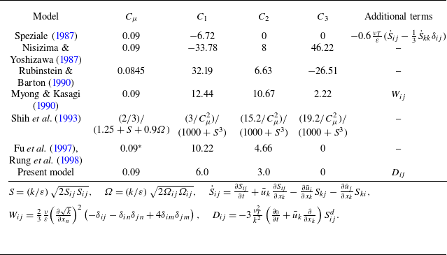
. Table 1 lists the proposed values for these coefficients in several typical quadratic NLEVMs.
Coefficients in typical quadratic NLEVMs.

*In the original model of Fu et al. (Reference Fu, Wang, Rung and Thiele1997) and Rung et al. (Reference Rung, Thiele and Fu1998), this coefficient depends on the local mean strain rates. For ease of comparison, it is set to 0.09 here.
Typically, the coefficients in NLEVMs are determined by considering the prediction of shear stress in simple shear flows or other complex flows. It is evident that the optimised sets of coefficients proposed for
 ${C_1}{-}{C_3}$
can vary significantly, depending on the specific flow or flow feature chosen for prediction. Remarkably, the present model, which is theoretically derived from the Fokker–Planck equation for turbulence, yields coefficients that are quantitatively close to those of established NLEVMs, particularly the quasi-realisable quadratic EVM of Fu et al. (Reference Fu, Wang, Rung and Thiele1997) and Rung et al. (Reference Rung, Thiele and Fu1998). Additionally, a notable feature of the present quadratic model is that there is no contribution from
 ${\Omega _{ik}}{\Omega _{jk}} - 1/3{\Omega _{lk}}{\Omega _{lk}}{\delta _{ij}}$
. This finding aligns with the prediction of Speziale (Reference Speziale1987), which demonstrated that such a quadratic rate-of-rotation tensor contribution leads to erroneous predictions for isotropic turbulence subjected to a solid-body rotation.
3.2. Comparison with experiments
The performance of the present nonlinear model is evaluated across three test cases: one incompressible and two compressible. The calculations are performed using the open-source software OpenFOAM (Jasak et al. Reference Jasak, Jemcov and Tuković2007), version 10. For the incompressible case, the solver simpleFoam is utilised. For the compressible cases, we use a modified density-based solver, ausmpwTurbulentFoam (Zhang Reference Zhang2021), which is adapted from rhoCentralFoam (Greenshields et al. Reference Greenshields, Weller, Gasparini and Reese2010) and employs the AUSMPW+ scheme (Kim et al. Reference Kim, Kim and Rho2001) for the convection terms to reduce numerical dissipation. The remaining terms are discretised similarly to those in rhoCentralFoam. Specifically, a second-order central scheme is applied for diffusion terms, while a second-order total variation diminishing method with the van Albada et al. (Reference van Albada, Van Leer and Roberts1982) limiter is used for cell face interpolations to ensure solution boundedness.
The new models are implemented based on two well-established
 $k\text{-}\varepsilon$
models: the Launder & Sharma (Reference Launder and Sharma1974) linear model and the Craft et al. (Reference Craft, Launder and Suga1996) cubic model. We replace the Reynolds stress constitutive relationship with (3.1), while retaining all other coefficients from these two models to ensure a fair comparison. In the following, we denote the new quadratic model based on the Launder & Sharma (Reference Launder and Sharma1974) model as ‘new model (1)’ and the new quadratic model based on the Craft et al. (Reference Craft, Launder and Suga1996) model as ‘new model (2)’.
To accurately capture the pronounced non-equilibrium effects in the shock-wave–boundary-layer interaction (SWBLI) cases, a specifically designed source term is introduced in the dissipation rate equation to control the excessive turbulent length scale in the SWBLI region. The source term is formulated as
 \begin{equation} {S_{\varepsilon cm}} = H Y{\lambda _l}\frac {{{{\tilde \varepsilon }^2}}}{k}, \end{equation}
where the homogeneous dissipation rate
 $\tilde \varepsilon$
is defined as
 $\tilde \varepsilon = \varepsilon - 2\nu { ( {\partial {k^{1/2}}/\partial {x_j}} )^2}$
. Here,
 $H$
is a calibration constant determined from numerical experiments, with recommended value 3. The term
 ${\lambda _l} = \max ( { ( {k/\tilde \varepsilon } ) ( {\partial {u_k}/\partial {x_k}} ), - 0.5} )$
is associated with velocity divergence, which vanishes in incompressible cases, and the coefficient
 $-0.5$
is introduced to maintain numerical stability. The switch function
 $Y = \tanh ( {2 ( {\eta - 3} )} ) - 1$
restricts the correction term to be primarily active in the near-wall viscous region, where
 $\eta = \max ( {\hat S,\hat \Omega } )$
, with
 $\hat S = ( {k/\tilde \varepsilon } )\sqrt {2S_{ij}^dS_{ij}^d}$
and
 $\hat \Omega = ( {k/\tilde \varepsilon } )\sqrt {{2\Omega _{ij}}{\Omega _{ij}}}$
. As demonstrated by Zhang et al. (Reference Zhang, Craft and Iacovides2022), incorporating this source term significantly mitigates the severe overprediction of wall heat flux in the SWBLI region, while exerting only a limited influence on wall pressure distributions and flow separation. Consequently, the overall results remain in good agreement with experimental measurements. Notably, the magnitude of the correction is determined directly by the velocity divergence, thereby accounting for compressibility effects.
Although numerous compressibility corrections have been proposed, their effectiveness and general applicability remain open questions. Some researchers advocate incorporating these compressibility corrections into their turbulence models. For example, Wang & Fu (Reference Wang and Fu2011) and Fu & Wang (Reference Fu and Wang2013) integrated the dilatation–dissipation corrections proposed by Sarkar et al. (Reference Sarkar, Erlebacher, Hussaini and Kreiss1991) and Sarkar (Reference Sarkar1995) into their
 $k{-}\omega{-}\gamma$
transition/turbulence model. This model has demonstrated remarkable success in engineering applications, and has been employed effectively to predict boundary layer transition in vehicles operating across a broad speed range, from subsonic to hypersonic. Conversely, some researchers suggest that incorporating these compressibility corrections is unnecessary for wall-bounded flows, as compressibility effects are generally not significant over a broad range of Mach numbers, and most turbulence models can already provide reasonably accurate predictions (So et al. Reference So, Gatski and Sommer1998; Wilcox Reference Wilcox1998; Rumsey Reference Rumsey2010). Additionally, DNS results (Huang et al. Reference Huang, Coleman and Bradshaw1995; Vreman et al. Reference Vreman, Sandham and Luo1996; Li et al. Reference Li, Komperda, Peyvan, Ghiasi and Mashayek2022) indicate that the associated terms are small or negligible. Given the ongoing debate on this issue, these compressibility corrections are not adopted in this study.
3.2.1. Two-dimensional backward-facing step
The first case is based on the experiment by Driver & Seegmiller (Reference Driver and Seegmiller1985), in which a series of laser Doppler velocimeter measurements were conducted for an incompressible turbulent flow over a backward-facing step in a diverging channel. Flow conditions upstream of the step were well developed, with a Reynolds number based on boundary layer momentum thickness 5000 at a location 4 step heights upstream of the step. The step height
 $H$
is set as 1.27 cm, the expansion rate is 1 : 9/8, and the molecular viscosity is
 $1.5 \times {10^{ - 5}}\,\mathrm{{m^2}\, s^{-1}}$
. In our calculation, the inflow length has been adjusted so that the naturally developing turbulent boundary layer on the lower wall grows to approximately the correct thickness and yields approximately the correct wall skin friction coefficient prior to the step. The inflow velocity is adjusted to yield the correct Mach number (
 $Ma=0.128$
) upstream of the step. Calculations are performed on a rectilinear mesh of approximately 60 000 cells, ensuring that the
 $y+$
value at the wall is less than unity.
Two-dimensional backward-facing step: comparison of velocity contours and streamlines for the four models. The arrow represents the reattachment point measured in the experiment.

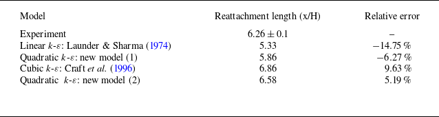
The reattachment length is a critical parameter for validating turbulence models in separated flow regions. We compare the reattachment lengths predicted by the four models with experimental measurements. As shown in figure 3, the Launder & Sharma (Reference Launder and Sharma1974) model predicts a shorter separating length, while the Craft et al. (Reference Craft, Launder and Suga1996) model seems to overestimate it. The two new quadratic models developed in this work demonstrate improved accuracy. A quantitative comparison is presented in table 2. It is shown that by replacing the Reynolds stress with the expression in (3.1), the relative error of the reattachment length for the Launder & Sharma (Reference Launder and Sharma1974) model decreases from 14.75 % to 6.27 %, and that of the Craft et al. (Reference Craft, Launder and Suga1996) model decreases from 9.63 % to 5.19 %.
Two-dimensional backward-facing step: comparison of reattachment length with the measured value for the four models.

Two-dimensional backward-facing step: comparison of computed and measured surface pressure and skin friction coefficients downstream of the step for the four models.

Axisymmetric compression corner: (a) the test model of the experiment of Kussoy & Horstman (Reference Kussoy and Horstman1989); (b) computational grid for the compression corner case.

Figure 4 compares the computed and measured surface pressure and skin friction coefficients downstream of the step. The pressure coefficients predicted by all four models are close to the experimental data. For the skin friction coefficients, the new model (1) demonstrates significant improvement over the original Launder & Sharma (Reference Launder and Sharma1974) linear model, while the new model (2), though essentially quadratic, performs comparably to the cubic Craft et al. (Reference Craft, Launder and Suga1996) model. These results highlight the effectiveness of the Reynolds stress relation derived from the turbulent Fokker–Planck equation proposed in this work.
3.2.2. Axisymmetric compression corner near
 $Ma=7$

The second case is based on the study by Kussoy & Horstman (Reference Kussoy and Horstman1989), who investigated the flow over axisymmetric ogive-cylinder-flares at Mach number 7.05. The test model used in his experiment is shown in figure 5(a). He considered a flare angle of
 $35^\circ$
, which represents a fully separated flow. The freestream temperature is 81.2 K, and the Reynolds number based on the nominal freestream conditions is 5,800,000 m−1.
The set-up of our study is the same as that of Zhang et al. (Reference Zhang, Craft and Iacovides2022). The computational grid, shown in figure 5(b), is a structured grid that is uniform in the streamwise direction and expands exponentially in the wall-normal direction. Both the cylinder and flare lengths are set to 20 cm, which is sufficient to cover the entire interaction region. The inlet boundary condition is determined by first calculating an undisturbed boundary layer flow over the cylinder and matching the measured and computed displacement thickness, which is 0.0074 m, at a point 6 cm upstream of the corner. A no-slip condition is applied to the wall, with the wall temperature fixed at 311 K, and zero gradient for pressure. Zero-gradient conditions are also applied to all variables at the outlet boundaries. Since the test model is axisymmetric, the ‘wedge’ boundary condition of OpenFOAM is used to run axisymmetric simulations with one cell in the circumferential direction and angle
 $1^\circ$
. The values of
 $y+$
at the first grid point off the wall are maintained below 0.1. A grid-independence test was conducted, showing that a mesh of
 $200\times200$
cells is sufficient to achieve numerically grid-independent results.
Axisymmetric compression corner: comparison of temperature contours and streamlines for the four models. The arrow represents the separating point measured in the experiment.

Axisymmetric compression corner: comparison of computed and measured surface pressure and heat flux at the wall for the four models.

The temperature contours and streamlines predicted by the four models are shown in figure 6. The Launder & Sharma (Reference Launder and Sharma1974) model and the new model (1) both predict a later separation, while the Craft et al. (Reference Craft, Launder and Suga1996) model and the new model (2) predict an earlier separation. For a quantitative comparison, as shown in figure 7, the surface pressure and heat flux predicted by the new model (1) are closer to the experimental values than those predicted by the Launder & Sharma (Reference Launder and Sharma1974) linear model. Specifically, the Launder & Sharma (Reference Launder and Sharma1974) model overestimates the peak wall heat flux by approximately 24 %, while the new model (1) overestimates it by only 8 %. This aligns with the findings of Friedrich & Bertolotti (Reference Friedrich and Bertolotti1996), who observed that compressibility effects enhance the anisotropy of the Reynolds stress due to turbulent fluctuations, and that NLEVMs provide a better foundation than linear models for improving predictions of compressibility effects. The results of the new model (2) are shown to be quite accurate and comparable to those of the cubic model, despite being only quadratic.
3.2.3. Two-dimensional impinging shock near
$Ma=8$

The third case is based on the experiment conducted by Kussoy & Horstman (Reference Kussoy and Horstman1991), which involved a two-dimensional impinging shock generated by a shock generator with turning angle
 $10^\circ$
. The test model is shown in figure 8(a). The free stream conditions are Mach number 8.18, pressure 430 Pa, temperature 81 K, and velocity 1446 m s−1. In our calculation, the shock generator is included in the computational domain, as shown in figure 8(b). A structured grid with
 $570\times180$
cells is used to discretise the flow field. The grid points in the streamwise direction are clustered at the leading edge of the shock generator, uniformly distributed in the interaction region, and grow exponentially in the wall-normal direction. The inlet boundary conditions are set to ensure that the displacement thickness at a specified station, 47 cm behind the leading edge of the shock generator, matches the measured value, i.e. 1.59 cm. The inlet profiles are obtained from a separate calculation of undisturbed boundary layer flow on a flat plate. Zero-gradient conditions are applied to all variables at the outlet boundary. At the wall, a no-slip condition is applied, with the temperature fixed at the experimental value 300 K, and a zero-gradient condition for pressure.
Two-dimensional impinging shock: (a) the test model of the experiment of Kussoy & Horstman (Reference Kussoy and Horstman1991); (b) computational grid for the impinging shock case.

Two-dimensional impinging shock: comparison of pressure contours and separation bubbles for the four models.

The pressure contours and the separation bubbles predicted by the four models are presented in figure 9. The Launder & Sharma (Reference Launder and Sharma1974) model and the new model (1) both predict a small separation bubble, while the Craft et al. (Reference Craft, Launder and Suga1996) model and the new model (2) predict a larger one. Figure 10 compares the computed surface pressure and heat flux at the wall with experimental measurements. It appears that higher-order terms play a minor role in this situation. The pressure profiles downstream of the interaction region are well predicted by all models, although the initial pressure rise predicted by the Launder & Sharma (Reference Launder and Sharma1974) model and the new model (1) is slightly underpredicted. The wall heat flux predicted by the Craft et al. (Reference Craft, Launder and Suga1996) model and the new model (2) fits the data very well, whereas the Launder & Sharma (Reference Launder and Sharma1974) model and the new model (1) predict a slightly higher peak wall heat flux.
Two-dimensional impinging shock: comparison of computed and measured surface pressure and heat flux at the wall for the four models.

4. Conclusions and discussions
In this study, we proposed a Fokker–Planck equation for turbulence based on the analogy with molecules described by kinetic theory. This equation aims to characterise turbulent flows at the hydrodynamic level and can be viewed as a specific instance of Pope’s GLM. We established a connection between the turbulent Fokker–Planck equation and the Reynolds stress constitutive relationship using the Chapman–Enskog expansion. When truncated to the zeroth order, the obtained solution corresponds to the isotropic part of the Reynolds stress. The first-order expansion yielded the well-known linear eddy viscosity model (EVM), while the second-order expansion resulted in a quadratic Reynolds stress constitutive relationship that also accounts for history effects.
We compared the coefficients of the quadratic Reynolds stress model with those of typical NLEVMs, and found them to be qualitatively consistent. Additionally, we implemented this quadratic Reynolds stress model in CFD codes and calculated three typical cases: a two-dimensional backward-facing step, an axisymmetric compression corner near Mach 7, and an impinging shock near Mach 8. The results indicate that the kinetic-based NLEVM developed in this work, without the use of ad hoc parameters in the Reynolds stress relationship, outperforms the traditional EVM and is comparable to a cubic model for two-dimensional flows.
Our efforts demonstrated the potential of deriving turbulence models from a kinetic perspective. Traditional models often struggle with the lack of scale separation between mean and fluctuating fields in the NS equations when incorporating eddy viscosity. In contrast, kinetic theory does not rely on scale separation, offering a distinct advantage in turbulence modelling. We demonstrated that turbulence models can be effectively encapsulated within a kinetic equation for turbulence. Compared to the similar work conducted by Chen et al. (Reference Chen, Kandasamy, Orszag, Shock, Succi and Yakhot2003, Reference Chen, Orszag, Staroselsky and Succi2004), which treats turbulent motion as a BGK-type relaxation process, describing turbulent motion as a stochastic process governed by a Fokker–Planck equation appears to be a more suitable approach. In this study, we expanded the turbulent Fokker–Planck equation to second order. As noted by Launder (Reference Launder1996), the introduction of nonlinear terms at the quadratic level proved insufficient for accurately capturing the effects of streamline curvature and the behaviour of three-dimensional flows. Notably, the same methodology can be used to perform higher-order expansions, generating additional terms to further refine the model.
As highlighted in § 2.1, there are two fundamentally different approaches to deriving turbulence models from kinetic theory. The approach adopted in this study involves first establishing a coarse-grained kinetic equation at the hydrodynamic level, then applying the Chapman–Enskog expansion to derive the constitutive relationship between Reynolds stress and average flow variables. The key challenge in this method lies in constructing the coarse-grained kinetic equation. In this study, we address this challenge by drawing an analogy between turbulent dynamics and Brownian motion. A more rigorous approach, such as directly coarse-graining the kinetic equation for molecules, remains a challenging yet promising area for future research.
Acknowledgements
The authors would like to thank Xiaoyong Wang and Jinglei Xu for valuable suggestions. The authors would also like to thank Xinliang Li and Ji Zhang for many helpful discussions.
Funding
This work was supported by the National Natural Science Foundation of China (grant nos 92371102 and 12272028).
Declaration of interests
The authors report no conflict of interest.
Appendix A. Moments of the Fokker–Planck equation for turbulence
From the Fokker–Planck equation for turbulence, i.e. (2.6), the corresponding moment equations can be straightforwardly derived.
We firstly multiply both sides of (2.6) by a generalised property function
 $Q$
, which is a function of the particle velocity and is therefore independent of space and time. Then integrating the product over the entire velocity space yields the extended moment equation
 \begin{equation} \frac {{\partial ( {n\bar Q} )}}{{\partial t}} + \frac {{\partial ( {n\overline {Q{u_k}} } )}}{{\partial {x_k}}} - n\frac {1}{\rho }\frac {{\partial {\sigma _{ij}}}}{{\partial {x_j}}}\frac {{\partial \bar Q}}{{\partial {u_i}}} = \Delta \left [ Q \right ]. \end{equation}
In (A1), the source term
 $\Delta [ Q ]$
is defined as
 \begin{equation} \Delta \left [ Q \right ] = \int _{{R^3}} {Q \left ( {\frac {1}{{{\tau _T}}}\frac {\partial }{{\partial {u_k}}} [ {f( {{u_k} - {{\bar u}_k}} )} ] + \frac {{2k}}{{3{\tau _T}}}\frac {{{\partial ^2}f}}{{\partial {u_k}\,\partial {u_k}}}} \right )} \mathrm{d}\boldsymbol{u}. \end{equation}
If
 $Q$
is taken as mass
 $m$
and fluid particle velocity
 $u_i$
, respectively, then the source terms vanish and the RANS equations at the average flow field level are recovered, i.e.
 \begin{equation} \left \{ \begin{aligned} &\frac {{\partial \rho }}{{\partial t}} + \frac {{\partial \rho {{\bar u}_j}}}{{\partial {x_j}}} = 0,\\[4pt] &\frac {{\partial {{\bar u}_i}}}{{\partial t}} + {{\bar u}_j}\frac {{\partial {{\bar u}_i}}}{{\partial {x_j}}} - \frac {1}{\rho }\frac {{\partial {\sigma _{ij}}}}{{\partial {x_j}}} - \frac {1}{\rho }\frac {{\partial {\sigma _{ij}^T}}}{{\partial {x_j}}} = 0. \end{aligned} \right . \end{equation}
In (A3),
 ${\sigma _{ij}^T} = - \overline {\rho {u'_i}{u'_j}}$
is the Reynolds stress.
If
 $Q$
is taken as
 ${u_i}{u_j}$
, and we simplify the resulting equation using (A3), then a partially modelled Reynolds stress transport equation can be obtained:
 \begin{equation} \frac {{D\overline {{u'_i}{u'_j}} }}{{Dt}} + \frac {{\partial \overline {{u'_i}{u'_j}{u'_k}} }}{{\partial {x_k}}} = {P_{ij}} + \frac {1}{\rho }\frac {{\partial {\sigma _{mn}}}}{{\partial {x_n}}}\frac {{\partial \overline {{u'_i}{u'_j}} }}{{\partial {u_m}}} - \frac {2}{{{\tau _T}}}\overline {{u'_i}{u'_j}} + \frac {4}{3}\frac {k}{{{\tau _T}}}{\delta _{ij}}. \end{equation}
The first three terms, representing mean convection, turbulent transport and production, are exact. When comparing (A4) with the exact Reynolds stress transport equation, and neglecting the viscous and pressure transport terms, the corresponding redistribution and dissipation terms are modelled as
 \begin{equation} {R_{ij}} - {\varepsilon _{ij}} = \frac {1}{\rho }\frac {{\partial {\sigma _{mn}}}}{{\partial {x_n}}}\frac {{\partial \overline {{u'_i}{u'_j}} }}{{\partial {u_m}}} - \frac {2}{{{\tau _T}}}\overline {{u'_i}{u'_j}} + \frac {4}{3}\frac {k}{{{\tau _T}}}{\delta _{ij}}. \end{equation}
Taking dissipation to be isotropic, the pressure rate of strain model implied by the Fokker–Planck equation for turbulence is
 \begin{equation} {R_{ij}} = \frac {1}{\rho }\frac {{\partial {\sigma _{mn}}}}{{\partial {x_n}}}\frac {{\partial \overline {{u'_i}{u'_j}} }}{{\partial {u_m}}} - \frac {2}{{{\tau _T}}}\overline {{u'_i}{u'_j}} + \left ( {\frac {4}{3}\frac {k}{{{\tau _T}}} + \frac {2}{3}\varepsilon } \right ){\delta _{ij}}. \end{equation}
The requirement that
 $R_{ij}$
be redistributive (i.e.
 ${R_{ii}} = 0$
) leads to the dissipation rate as
 \begin{equation} \varepsilon = - \frac {1}{\rho }\frac {{\partial {\sigma _{mn}}}}{{\partial {x_n}}}\frac {{\partial k}}{{\partial {u_m}}}, \end{equation}
which indicates that the dissipation of turbulent kinetic energy is related to molecular viscosity.
Appendix B. The eigenfunctions of the Fokker–Planck operator
The Fokker–Planck operator, defined as
 \begin{equation} L\left [ Q \right ] = \frac {1}{{{f_M}}}\frac {\partial }{{\partial {u_i}}}\left [ {\frac {2}{3}k \, {f_M}\frac {\partial }{{\partial {u_i}}}\left ( Q \right )} \right ], \end{equation}
is a linear operator. Its eigenfunctions, denoted by
 $Q$
, possess the property
 \begin{equation} L\left [ Q \right ] = \lambda Q, \end{equation}
where
 $\lambda$
are the corresponding eigenvalues. To obtain solutions for the Chapman–Enskog expansion of the Fokker–Planck model, we identify several eigenfunctions as follows:
 \begin{align} &{A_{ij}} = {u'_i}{u'_j} - \frac {1}{3}{u'_k}{u'_k}{\delta _{ij}},\end{align}
 \begin{align} &{B_j} = {u'_j}\left ( \frac {\boldsymbol{u}^{\prime 2}}{2} - \frac {5}{2} \, \frac {2}{3}k \right ),\end{align}
 \begin{align} &{Q_{{E_1}}} = {u'_i}\frac {{\partial S_{ij}^d}}{{\partial {x_j}}},\end{align}
 \begin{align} &{Q_{{E_2}}} = \frac {{{u'_i}{u'_i}}}{{4k/3}} - \frac {3}{2},\end{align}
 \begin{align} &{Q_A} = {\left ( {{u'_i}{u'_j}\frac {{\partial {{\bar u}_i}}}{{\partial {x_j}}} - \frac {1}{3}{u'_m}{u'_m}\frac {{\partial {{\bar u}_i}}}{{\partial {x_j}}}{\delta _{ij}}} \right )^2}, \end{align}
 \begin{align} &{Q_{{B_1}}} = {u'_i}{u'_j} - \frac {1}{3}{u'_k}{u'_k}{\delta _{ij}}, \end{align}
 \begin{align} &{Q_{{B_2}}} = {u'_l}\frac {\partial }{{\partial {x_l}}}\left ( {\frac {{\partial {{\bar u}_i}}}{{\partial {x_j}}}} \right ) \left ( {{u'_i}{u'_j} - \frac {1}{3}{u'_k}{u'_k}{\delta _{ij}}} \right ), \end{align}
 \begin{align} &{Q_C} = \left ( {{u'_l}{u'_j}\frac {{\partial {{\bar u}_i}}}{{\partial {x_l}}} + {u'_l}{u'_i}\frac {{\partial {{\bar u}_j}}}{{\partial {x_l}}} - \frac {2}{3}{u'_k}{u'_l}\frac {{\partial {{\bar u}_k}}}{{\partial {x_l}}}{\delta _{ij}}} \right )\frac {{\partial {{\bar u}_i}}}{{\partial {x_j}}}, \end{align}
 \begin{align} &{Q_{{D_1}}} = \frac {1}{\rho }\frac {{\partial {\sigma _{lj}}}}{{\partial {x_j}}}{u'_l}\left ( {{u'_i}{u'_j} - \frac {1}{3}{u'_k}{u'_k}{\delta _{ij}}} \right )\frac {{\partial {{\bar u}_i}}}{{\partial {x_j}}}, \end{align}
 \begin{align} &{Q_{{D_2}}} = \frac {1}{\rho }\frac {{\partial {\sigma _{lj}}}}{{\partial {x_j}}}\left ( {{u'_j}\frac {{\partial {{\bar u}_l}}}{{\partial {x_j}}} + {u'_i}\frac {{\partial {{\bar u}_i}}}{{\partial {x_l}}} - \frac {2}{3}{u'_l}{\delta _{ij}}\frac {{\partial {{\bar u}_i}}}{{\partial {x_j}}}} \right ), \end{align}
 \begin{align} &D = \frac {\partial }{{\partial {x_j}}}\left ( {\frac {{\partial {{\bar u}_i}}}{{\partial {x_j}}}} \right ){u'_i} + \frac {\partial }{{\partial {x_i}}}\left ( {\frac {{\partial {{\bar u}_i}}}{{\partial {x_j}}}} \right ){u'_j} - \frac {2}{3}\frac {\partial }{{\partial {x_m}}}\left ( {\frac {{\partial {{\bar u}_i}}}{{\partial {x_j}}}} \right ){u'_m}{\delta _{ij}}, \end{align}
 \begin{align} &M = {u'_i}{u'_s}\frac {{\partial {{\bar u}_i}}}{{\partial {x_m}}}\frac {{\partial {{\bar u}_s}}}{{\partial {x_m}}} + {u'_j}{u'_s}\frac {{\partial {{\bar u}_m}}}{{\partial {x_j}}}\frac {{\partial {{\bar u}_s}}}{{\partial {x_m}}} - \frac {2}{3}{u'_m}{u'_s}\frac {{\partial {{\bar u}_n}}}{{\partial {x_n}}}\frac {{\partial {{\bar u}_s}}}{{\partial {x_m}}} \nonumber \\[6pt] &\qquad {}+ {u'_i}{u'_t}\frac {{\partial {{\bar u}_i}}}{{\partial {x_m}}}\frac {{\partial {{\bar u}_m}}}{{\partial {x_t}}} + {u'_j}{u'_t}\frac {{\partial {{\bar u}_m}}}{{\partial {x_j}}}\frac {{\partial {{\bar u}_m}}}{{\partial {x_t}}} - \frac {2}{3}{u'_m}{u'_t}\frac {{\partial {{\bar u}_n}}}{{\partial {x_n}}}\frac {{\partial {{\bar u}_m}}}{{\partial {x_t}}} \end{align}
 \begin{align} &\qquad {}- \frac {2}{3}{u'_i}{u'_m}\frac {{\partial {{\bar u}_i}}}{{\partial {x_m}}}\frac {{\partial {{\bar u}_n}}}{{\partial {x_n}}} - \frac {2}{3}{u'_j}{u'_m}\frac {{\partial {{\bar u}_m}}}{{\partial {x_j}}}\frac {{\partial {{\bar u}_n}}}{{\partial {x_n}}} + \frac {4}{9}{u'_k}{u'_k}\frac {{\partial {{\bar u}_m}}}{{\partial {x_m}}}\frac {{\partial {{\bar u}_n}}}{{\partial {x_n}}}, \nonumber \\[6pt] &N = \frac {{\partial {{\bar u}_k}}}{{\partial {x_m}}}\frac {{\partial {{\bar u}_k}}}{{\partial {x_m}}} + \frac {{\partial {{\bar u}_k}}}{{\partial {x_m}}}\frac {{\partial {{\bar u}_m}}}{{\partial {x_k}}} - \frac {2}{3}\frac {{\partial {{\bar u}_m}}}{{\partial {x_m}}}\frac {{\partial {{\bar u}_k}}}{{\partial {x_k}}}. \\[6pt] \nonumber \end{align}
It is straightforward to demonstrate that
 \begin{align} L\left [ {{A_{ij}}} \right ] &= - 2{A_{ij}},\nonumber\\[4pt] L\left [ {{B_j}} \right ] &= - 3{B_j},\nonumber\\[4pt]L\left [ {{Q_{{E_1}}}} \right ] &= - {Q_{{E_1}}},\nonumber\\[4pt]L\left [ {{Q_{{E_2}}}} \right ] &= - 2{Q_{{E_2}}},\nonumber\\[4pt] L\left [ {{Q_A}} \right ] &= - 4{Q_A} + 2\theta M,\nonumber\\[4pt] L\left [ {{Q_{{B_1}}}} \right ] &= - 2{Q_{{B_1}}},\nonumber\\[4pt]L\left [ {{Q_{{B_2}}}} \right ]& = - 3{Q_{{B_2}}} + 2\theta D, \nonumber\\[4pt] L\left [ {{Q_C}} \right ] &= - 2{Q_C} + 2\theta N,\nonumber\\[4pt]L\left [ {{Q_{{D_1}}}} \right ] &= - 3{Q_{{D_1}}} + \tfrac {4}{3}k{Q_{{D_2}}},\nonumber\\[4pt]L\left [ {{Q_{{D_2}}}} \right ] &= - 3{Q_{{D_2}}},\nonumber\\[4pt] L\left [ D \right ] &= - D,\nonumber\\[4pt] L\left [ M \right ] &= - 2M{\rm { + }}4\theta N,\nonumber\\[4pt]L\left [ N \right ] &= 0. \end{align}
By using these eigenfunctions, we can expand the distribution function in terms of the eigenfunctions of the Fokker–Planck operator, and obtain the coefficients through the Chapman–Enskog expansion.
Appendix C. The integrals of
${\boldsymbol{f}}^{\boldsymbol{( 2 )}}$
correspond to the Fokker–Planck equation for turbulence

The second-order expansion of the turbulent Fokker–Planck equation is expressed in (2.50). To derive the Reynolds stress up to second order, we integrate
 $m{u'_{\left \langle i \right .}}{u'_{\left . j \right \rangle }}$
with respect to the second-order distribution function
 $f^{ ( 2 )}$
, handling each component term by term, and then reformulate the results into tensorial form. The relevant integrals are computed and presented as follows:
 \begin{align} \int _{{R^3}} {mu{'_{\left \langle i \right .}}u{'_{\left . \! j \right \rangle }}{f_M}}& \left [ { - \frac {4}{3}k \, {Q_{{E_1}}}} \right ]\mathrm{d}\boldsymbol{u}' = 0, \end{align}
 \begin{align} \int _{{R^3}} {mu{'_{\left \langle i \right .}}u{'_{\left .\! j \right \rangle }}{f_M}}& \left [ { - \frac {4}{9}k \, S_{ij}^d\frac {{\partial {{\bar u}_i}}}{{\partial {x_j}}} \, {Q_{{E_2}}}} \right ]\mathrm{d}\boldsymbol{u}' = 0, \end{align}
 \begin{align} \int _{{R^3}} {mu{'_{\left \langle i \right .}}u{'_{\left . \!j \right \rangle }}{f_M}}& \left [ {\frac {1}{{8k/3}} \, {Q_A}} \right ]\mathrm{d}\boldsymbol{u}' = \frac {1}{2}\rho {\left ( {\frac {2}{3}k} \right )^2} \nonumber \\[4pt] & \times \left [ {4\left ( {{S_{ik}}{S_{kj}} - \frac {2}{3}{S_{ij}}{S_{mm}}} \right ) - \frac {4}{3}\left ( {{S_{mn}}{S_{mn}} - \frac {2}{3}{S_{mm}}{S_{nn}}} \right ){\delta _{ij}}} \right ], \end{align}
 \begin{align} \int _{{R^3}} {mu{'_{\left \langle i \right .}}u{'_{\left . \!j \right \rangle }}{f_M}}& \frac {1}{2}\left [ {\frac {{{\partial _0}}}{{\partial t}}\left ( {\frac {{\partial {{\bar u}_i}}}{{\partial {x_j}}}} \right ) + {{\bar u}_l}\frac {\partial }{{\partial {x_l}}}\left ( {\frac {{\partial {{\bar u}_i}}}{{\partial {x_j}}}} \right )} \right ] {Q_{{B_1}}}\mathrm{d}\boldsymbol{u}' = \rho {\left ( {\frac {2}{3}k} \right )^2}\left ( {\frac {{{\partial _0}}}{{\partial t}} + {{\bar u}_l}\frac {\partial }{{\partial {x_l}}}} \right )S_{ij}^d, \end{align}
 \begin{align} \int _{{R^3}} {mu{'_{\left \langle i \right .}}u{'_{\left .\! j \right \rangle }}{f_M}}& \left [ {\frac {1}{3} \, {Q_{{B_2}}}} \right ]\mathrm{d}\boldsymbol{u}' = 0, \end{align}
 \begin{align} \int _{{R^3}} {mu{'_{\left \langle i \right .}}u{'_{\left . \! j \right \rangle }}{f_M}}& \left [ { - \frac {1}{2} \, {Q_C}} \right ]\mathrm{d}\boldsymbol{u}' = - \rho {\left ( {\frac {2}{3}k} \right )^2} \nonumber \\[4pt] & \times \left [ {{S_{ik}}\frac {{\partial {{\bar u}_k}}}{{\partial {x_j}}} + {S_{jk}}\frac {{\partial {{\bar u}_k}}}{{\partial {x_i}}} - \frac {2}{3}{S_{ij}}{S_{mm}} - \frac {2}{3}\left ( {{S_{mn}}{S_{mn}} - \frac {1}{3}{S_{mm}}{S_{nn}}} \right ){\delta _{ij}}} \right ], \end{align}
 \begin{align} \int _{{R^3}} {mu{'_{\left \langle i \right .}}u{'_{\left .\! j \right \rangle }}{f_M}}& \left [ {\frac {4}{9}k \, {Q_{{D_1}}}} \right ]\mathrm{d}\boldsymbol{u}' = 0, \end{align}
 \begin{align} \int _{{R^3}} {mu{'_{\left \langle i \right .}}u{'_{\left .\! j \right \rangle }}{f_M}}& \left [ {\frac {4}{9}k \, {Q_{{D_2}}}} \right ]\mathrm{d}\boldsymbol{u}' = 0, \end{align}
 \begin{align} \int _{{R^3}} {mu{'_{\left \langle i \right .}}u{'_{\left .\! j \right \rangle }}{f_M}}& \left [ {\frac {4}{9}k \, D} \right ]\mathrm{d}\boldsymbol{u}' = 0, \end{align}
 \begin{align} \int _{{R^3}} {mu{'_{\left \langle i \right .}}u{'_{\left .\! j \right \rangle }}{f_M}}& \left [ {\frac {1}{4} \, M} \right ]\mathrm{d}\boldsymbol{u}' = 2\rho {\left ( {\frac {2}{3}k} \right )^2} \nonumber \\[4pt] &{}\times \left [ {\left ( {{S_{ik}}{S_{kj}} - \frac {2}{3}{S_{ij}}{S_{mm}}} \right )} \right ] - \frac {1}{3}\left ( {{S_{mn}}{S_{mn}} - \frac {2}{3}{S_{mm}}{S_{nn}}} \right ){\delta _{ij}}. \\[6pt] \nonumber \end{align}
The expressions for eigenfunctions such as
 $Q_{{E_1}}$
,
 $Q_{{E_2}}$
and others are given in Appendix B. Summarising these integrals, we obtain the second-order Reynolds stress. After reorganisation, the result can be expressed as
 \begin{equation} \begin{aligned} \sigma _{ij}^{T\left ( 2 \right )} =& - \frac {1}{2}\rho \tau _T^2 \left ( {\frac {2}{3}k} \right ) \left ( {\frac {{{\partial _0}}}{{\partial t}} + {{\bar u}_k}\frac {\partial }{{\partial {x_k}}}} \right )S_{ij}^d \\[4pt] &{}- \rho \tau _T^2 \left ( {\frac {2}{3}k} \right ) \left ( {S_{ik}^dS_{kj}^d - \frac {1}{3}S_{mn}^dS_{mn}^d{\delta _{ij}}} \right ) + \frac {1}{2}\rho \tau _T^2 \left ( {\frac {2}{3}k} \right ) ( {S_{ik}^d{\Omega _{kj}} + S_{jk}^d{\Omega _{ki}}} ). \end{aligned} \end{equation}