NUTRITIONAL STATUS, BODY STATURE, AND BIOLOGICAL STANDARD OF LIVING

Anthropometry provides one of the best tools to assess nutritional and health status. There is a biological relationship between nutrition and health on the one hand and the physical development of children on the other. To the human body, nutritional intake and body reserves provide energy which is absorbed for the maintenance of vital body functions (breathing, heart rate, and so on), diseases (raised body temperature, bodily wastes, parasites, and so on), physical activities, and body growth. The latter acts as a buffer, when intakes are low or energy expenditures are high.Footnote ¹⁰ For the transformation of energy into body growth, certain micronutrients like iron, calcium, iodine, or vitamin A, are also essential. Accordingly, the body fails to grow at a normal rate as a result of chronically insufficient intakes—in terms of both quantity and quality—and a high burden of diseases and physical exertion. Mean height can be considered an indicator of a population's nutritional and health status.

Final adult height registers height increments cumulatively from fetal origins to maturity.Footnote ¹¹ However, not every phase of growth is equally important. A large share of total height is acquired in the first three years of life.Footnote ¹² It is also this period, when children are weaned, that they have quantitatively and qualitatively high energy needs and are highly vulnerable to infections caused by unhygienic conditions or contaminated food.Footnote ¹³ For this reason, deprived children typically fall behind in the early years of life. In principle, children can catch-up the shortfall in growth later if conditions do markedly improve.Footnote ¹⁴ However, because socioeconomic and nutritional conditions often persist, such catch-up is unusual, so that much of the variation in adult height is set by age four.Footnote ¹⁵

The anthropometry based indicator has several advantages. Heights measure outcomes, not inputs.Footnote ¹⁶ They do not, for example, discriminate against certain foodstuffs; what matters is whether the diet is sufficient to meet the bodily needs of growing children; a mixture of leaves, groundnuts, and beans, and a good grain staple can together make up a suitable source of nutrients, although animal products such as milk, meat, fish, and eggs often proved to be more effective. Furthermore, mean heights are responsive to distributional effects. Heights are subject to a decreasing marginal product. In other words, the height increment resulting from additional expenditures on nutrition and health will decrease with higher levels of consumption of nutrition and health inputs. Therefore, mean heights will decrease when redistributing inputs from the poor to the rich. Finally, it is not assumed that there is only one pattern of development. Height measurements are applicable to the diverse social and economic systems that existed in Kenya including hunters, pastoralists, subsistence farmers, cash crop producers, and employees in the modern and informal sector. This implies that mean height is a consistent measure over time.

Kenya's population is ethnically diverse.Footnote ¹⁷ What role does genetics play for heights? Genetics does indeed have a strong influence on heights of individuals—it is expressed in the variance of individual heights that can be observed when individuals grow up under relatively equal conditions. However, when mean heights of populations are considered, the “noise” of individual genetics cancels. Large height differences were found between rich and poor people of the same ethnic group more so than between socioeconomic elites of different ethnic backgrounds that grew up under good environmental conditions.Footnote ¹⁸ Moreover, average heights vary considerably within the major ethnolinguistic groups in Kenya, the Bantu (Kamba, Kikuyu, Luhya, Meru, and Mijikenda), Nilotic (Luo, Kalenjin, Samburu, Turkana, and Maasai), and Cushitic (Somali), while there is considerable overlap in the range. Plausible explanations other than genetics exist for the differences in stature (in fact, ethnicity is a marker of spatial, economic, and social characteristics). Finally, the genetic pool of a population does not vary over short periods of time such as 10–50 years—mean height, on the other hand, does, if the environment has changed accordingly. By and large, environmental conditions are the determining factors of height differences between populations.

Heights must not be regarded narrowly as a measure of nutritional status. They have a much broader meaning. Children's body growth responds very sensitively to deprivation in essential human needs; that is, when they are exposed to hunger, low-nutrient diets, poor housing and sanitary conditions, contaminated food and water, no or limited access to medical care, and child labor. Thus, average stature is a biological indicator of social and economic development and as such it is a component of the Biological Standard of Living.Footnote ¹⁹

DATA

Historical sources of height measurements are diverse. Height was used for identification purposes and, as a measure of physical fitness, body stature was routinely taken in medical examinations, so that height data can be found for groups including prison, hospital, or school populations. Nutrition and health surveys frequently collected anthropometric data. Furthermore, anthropologists took a keen interest in the shape and body proportions of African ethnic groups. This study draws from these sources. The core data set, however, is derived from military records that have survived at the Defence Headquarters, Kenyan Armed Forces, Nairobi. Attestation papers and medical reports of 1,667 Kenyans enlisted in the British colonial forces provide details such as date of enlistment, regimental number, unit, place of birth, age, ethnicity, religion, the soldier's signature (if literate), and barefoot height.

Heights reveal the nutritional status only of those who were measured; the findings can only be generalized to the extent to which the sample represents the broader population. Can a selection of army recruits be considered sufficiently representative of Kenyan men? In the following, I summarize relevant facts about recruiting patterns, making special reference to the data set.

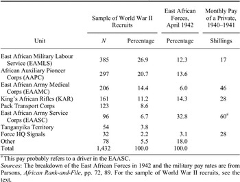
In peace time, the British colonial army in Kenya was a small force. There was no conscription and the army was extremely selective, recruiting soldiers from ethnic groups with supposedly inherent military qualities, the so-called “martial races.”Footnote ²⁰ In the 1920s and 1930s, martial races included the Kamba, Kalenjin, and Somali, pastoral and semi-pastoral groups from impoverished regions. In contrast, the Kikuyu and Meru of central Kenya were hardly found in the army. World War II brought a massive expansion of military personnel. From an interwar strength of less than 1,000 men, the armed forces increased to 75,000 by 1943. Thus, every tenth adult man was serving in the military, representing about 20 percent of the wage labor force.Footnote ²¹ The huge demand for able-bodied and skilled men was met by extending the recruitment pool to communities the British did not consider martial. Additionally, the military offered wages above civilian levels. In 1941 the pay ranged between 17 and 60 shillings per month for a newly trained private in the East African Military Labour Service (EAMLS) and East African Army Service Corps (EAASC) respectively, whereas civil wages for unskilled labor averaged between 8 and 12 shillings.Footnote ²² The military offered additional pulls such as uniforms, housing, food, professional training, and promotion. Understandably, military service was attractive for most men, except for those from very high status background in the proximity of Nairobi, who could find better paid urban employment.Footnote ²³

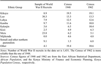
It appears that World War II recruits would provide a good coverage of ethnic and social backgrounds of Kenyan men. Therefore, this study focuses on World War II recruits who comprise 85 percent of the data set. The World War II subsample covers the larger ethnic groups in Kenya, and the geographic origins of the rank and file are widely spread (Figure 1). There are clusters of recruits born in places around Lake Victoria and in the Highlands north of Nairobi. Fewer recruits are from places in between, or from the northern parts of Kenya, but this is what one would expect considering the lower population density of these areas.Footnote ²⁴ The only apparent drawback is that coastal peoples (Mijikenda, Pokomo, Taita, Taveta, and Swahili) are almost entirely missing. The ethnic composition of the sample of World War II recruits thus does deviate slightly from that of the Kenyan population (Table 1). The Kikuyu are somewhat underrepresented, while Luo and Meru are overrepresented. However, since we are interested in differences between ethnic groups, their proportions are largely irrelevant. It is a much more crucial requirement that each ethnic group in the sample is sufficiently representative of each ethnic group in the population.

The East African Forces were a complex organization with specialized branches and therefore, a high degree of differentiation can be found within the army. The least skilled labor was pooled in labor units such as the EAMLS. The African Auxiliary Pioneer Corps (AAPC) took on somewhat more sophisticated works, but it was still generally composed of men who did not meet the physical and intelligence requirements of combatant and technical units.Footnote ²⁵ The healthiest recruits were sent to the frontline battalions of the King's African Rifles (KAR). Moreover, there were a number of support and specialist units that absorbed proficient and educated men such as the East African Army Service Corps (EAASC), which was responsible for motorized transport and logistics, the Signals Corps, and the East African Army Medical Corps (EAAMC). The different requirements and qualifications were also reflected in pay scales. The data set, though it does not concur completely, covers some of the diversity within the East African Forces (Table 2). Most of the recruits in the sample are from the EAMLS, which, however, does not count much, as their heights were seldom recorded.Footnote ²⁶ Next come the AAPC, EAAMC, and KAR. The data set also contains a substantial number of about 100 recruits of the EAASC and the Pack Transport Corps. These units account for 90 percent of the sample. Because they reflect the range of social and educational backgrounds of the men very well, membership to these units will later be used to explain height differences.

Figure 1

ETHNIC GROUP AND PLACE OF BIRTH AND ORIGIN OF KENYAN WORLD WAR II RECRUITS

Notes: Place of birth and origin from attestation papers were matched with entries in the Geographic Names Database of the National Geospatial-Intelligence Agency, from which latitude and longitude were retrieved. The database is the official repository of foreign place name decisions approved by the U.S. Board on Geographic Names. It was possible to locate 89 percent of World War II recruits from my sample of 1,439.Source: See the text.

Table 1

ETHNIC GROUPS IN THE SAMPLE OF WORLD WAR II RECRUITS AND THE KENYAN POPULATION (in percent)

Notes:

Number of World War II recruits in the data set is 1,431. The Census of 1962 is more reliable than the one of 1948.

Sources:

Census figures of 1948 and 1962 are from the East African Statistical Department, African Population, and the Kenya Ministry of Finance and Economic Planning, Kenya Population Census, respectively.

Despite the demand for recruits and the wide variety of employment opportunities, the army did not accept everyone. The most unfit men were certainly rejected on medical grounds. Official standards, which varied between units and changed over time, were also in place for age, height, weight, eyesight, and intelligence. Beyond the requirement of an age between 18 and 40, the most critical restriction was the minimum height requirement (MHR). T. Farnworth Anderson, a medical officer who served with the forces, reported that stunted growth was a frequent cause of rejection.Footnote ²⁷ As short recruits were sorted out, available height measurements represent the taller men in the population. This is a potential source of bias. Fortunately, econometric techniques exist to overcome the problem, via a procedure that will be explained in the next section. Furthermore, the data set does not include soldiers who were killed in action or died from accidents and disease. Because of the relatively low casualty rate of 3 percent, biases from this source are likely to be negligible.Footnote ²⁸ To conclude, the recruiting pattern of World War II makes recruits an excellent sample that sufficiently represents the ethnic diversity and social backgrounds of a reasonably fit, male Kenyan wage labor force, aged 20–30 years.

Table 2

DESCRIPTIVES OF MILITARY UNITS, WORLD WAR II

# This pay probably refers to a driver in the EAASC.

Sources:

The breakdown of the East African Forces in 1942 and the military pay rates are from Parsons, African Rank-and-File, pp. 72, 89. For the sample of World War II recruits, see the text.

The sample of army recruits does not permit a thorough analysis of changes in height over a longer period of time.Footnote ²⁹ Therefore, a variety of other sources were consulted. The anthropologists Norman M. Leys and T. A. Joyce provide an excellent coverage of ethnic groups and a large sample of adult men born in the time before the colonial conquest (N = 622).Footnote ³⁰ They reported the measurement of each individual, and even though they did not give detailed background information on individuals, they describe their sample as “fairly representative of the racial types,” where height was considered a characteristic thereof. Specifically, Leys and Joyce procured their measurements at the town surgery in Mombasa, from trivial cases. Additionally, they took measurements from villagers at a mission station, and from political prisoners in Mombasa.Footnote ³¹ They also drew measurements from policemen and applicants for admission to the police force who, in their words, “were certainly above the tribal average in physique.”Footnote ³² The remark probably refers to the Indians, Somalis, Comorians, and Swahilis in their sample who predominated amongst the police rank and file at that time and which I do not use in my analaysis.Footnote ³³ I examined the reported height measurements, screening the height distributions for abnormal behaviours, but I could not find any apparent problems.Footnote ³⁴ Note that biases are unlikely, especially if one agrees that intra-ethnic height gradients were small at that time.

Furthermore, I make use of summary statistics of 1,271 physical examinations taken from 21–40 year old men in the Kikuyu Reserve published in John Boyd Orr and J. L. Gilks.Footnote ³⁵ For postindependence Kenya, anthropometric data was retrieved from the nationally representative Kenya Demographic and Health Survey 2003.Footnote ³⁶ The DHS survey provides data for women but not for men. Female heights are therefore transformed into male equivalents, an approach described in the next section and, in more detail, in the Appendix.

METHODOLOGY

Heights are most informative about conditions of nutrition and health in the first few years after birth. Many World War II recruits did not know their year of birth or their age. In these cases, their age was either estimated, described as “adult” or the entry was simply left blank. Using the available age data gives an average age at enlistment of 26.5 years. About 70 percent of the recruits were aged 20–35. Hence, most World War II recruits were born in the 1910–1920 period (Figure 2). The heights, therefore, refer to conditions during this period.

The army required recruits to pass a minimum height and short stature was indeed a frequent cause of rejection.Footnote ³⁷ The shortfall of recruits at the lower tail of the height distribution is a severe problem; without proper treatment, mean height estimates will be upwardly biased. Anthropometric historians were frequently confronted with deficient height distributions. From various techniques that were proposed to overcome the problem, truncated normal regression became the method of choice.Footnote ³⁸

Figure 2

YEAR OF BIRTH AND YEAR OF ENLISTMENT

Notes: The age was only recorded for a fraction of recruits. N(year of birth/year of enlistment): 610/1439. Mean age of recruits was 26.5 years old.Sources: See the text.

Truncated normal regression is a standard technique in econometrics.Footnote ³⁹ From an underlying data generating process of the form

the sample is restricted to those cases, where y is greater than the truncation point τ (in the left truncated situation). From assuming normality in the underlying process it follows that y has a truncated normal distribution in the sample data. Its density can be expressed as

where φ(.) and Φ(.) denote the standard normal pdf and cdf respectively. The maximum likelihood estimator (MLE) chooses the parameters β and σ that maximize the sum of logs of these densities. Truncated MLE is an unbiased, consistent, and asymptotically efficient estimator of β. Normality is a crucial assumption, which, however, reasonably holds for heights in homogeneous populations. In this study, we use an unconstrained MLE, where no ad hoc restrictions on the standard deviation σ of the underlying population are made.

To apply this technique, knowledge of the truncation point τ is needed, which in the case of truncated height samples corresponds to the MHR.Footnote ⁴⁰ According to medical handbooks, the prewar MHR was 5'7”.Footnote ⁴¹ In the course of the huge demand for soldiers in World War II, physical requirements were officially lowered to 5'3” except for the EAMLS, which dropped its requirement to 5'2” in 1942. The Signal Corps had no height requirement and recruits as young as 15 years old were accepted.Footnote ⁴² The recruits in the data set mostly enrolled between 1939 and 1941, when requirements may have been in transition. Moreover, there were a couple of exceptions and recruiters did not always pay attention to the guidelines. In order to determine the de facto truncation point, histograms are examined.Footnote ⁴³ Taking World War II recruits as a whole the histogram indicates a shortfall starting at 66 inches and growing at 64 inches (Figure 3, lower right panel). When distinguishing by branch, various truncation points can be observed (Figure 3).Footnote ⁴⁴ In particular, truncation points could be identified at 63 (EAAMC, General Hospital), 65 (PT Corps and Camel Transport, EAASC), and 66 (AAPC and KAR) inches. For the small number of recruits in the Signals, no MHR is assumed.Footnote ⁴⁵ Note that MHRs are well below the sample modes, a feature which enhances the reliability of the estimates.

Figure 3

HEIGHT DISTRIBUTIONS BY BRANCH OF SERVICE

Notes: Acronyms refer to branches of services; for full names, see Table 2. Bin width is one inch. Truncation point chosen is 63 inches for EAAMC, 65 inches for PT Corps and EAASC, and 66 inches for AAPC and KAR. About 22 percent of the available height measurements fall below the truncation points.Sources: See the text.

Using the sample of African army recruits, I will estimate the following regression models. The start will make a specification in which ethnic group is taken as the single predictor of mean height. Ethnicity is a fundamental clue to geographical origin (Figure 1). Taking ethnicity as regional entity also facilitates comparisons with other height data (Kenyan administrative units changed frequently). Next, I will test the effect of social and educational background on nutritional status. In particular, the recruit's ability to sign the attestation paper and branch membership are used as proxy variables. Note that literacy is a rather weak indicator of wealth. In pastoral societies before 1960, for example, education and wealth are not correlated, or even negatively correlated. Finally, for taking into account that environmental influences changed over time, variables are used that indicate the year of birth (in the case of the World War II army sample, birth years are restricted to the 1900–1920 period). In all three models, dummy variables for known ages 15–22 years are included in order to control for lower statures of individuals who had not attained their final adult height at the time of measurement.

For postindependence Kenya, only height data of women are used, since nutrition surveys collected extensive anthropometric data on this gender, allowing for the most comprehensive coverage of Kenyan ethnic groups. It is possible to predict male heights from female heights based on prevalent patterns of sexual dimorphism in stature.Footnote ⁴⁶ Admittedly, nutritional status of the genders does not perfectly correlate. Part of dimorphism in stature is made up by discriminatory environmental influences including differential resource allocation between girls and boys. The approach can nevertheless be justified on the grounds that the relationship is strong and that prediction errors are typically small. Boys and girls living in the same household are subject to many similar environmental conditions. Gender dimorphism in stature can therefore be expected to be much smaller than height differences over space, time or between social classes.Footnote ⁴⁷ Differences or changes in gender dimorphism are therefore unlikely to delude conclusions about secular trend in the heights of Kenyan ethnic groups. Female heights were transformed into male equivalents assuming a male to female ratio of 106.73 percent observed in a sample of African populations. This is a rather conservative estimate. Details of the derivation are presented in the Appendix.

A potential caveat for the long-term series 1880–1980 is that it is compiled from four cross sections, where birth cohorts do not overlap. Thus, there is a risk that the observed height differences partly reflect differences in the backgrounds of the sampled population rather than genuine changes over time. However, from what is known of the backgrounds, cohorts are comparable and major biases are not to be expected.

REGIONAL INEQUALITY: A CROSS SECTION OF WORLD WAR II RECRUITS

Mean stature estimates of World War II recruits indicate a pronounced regional inequality in nutritional and health status (Table 3, column 1). With an average height of 65.1 inches (165.4 cm), the

Table 3

DETERMINANTS OF HEIGHTS IN KENYAN WORLD WAR II RECRUITS: TRUNCATED NORMAL REGRESSION (in inches)

*** p<0.01

** p<0.05

* p<0.1

Notes:

Coefficients were estimated by maximum likelihood. Sigma denotes the estimated standard deviation of heights. See the text for details. Robust z-statistics in parentheses; all explanatory variables are dummy variables. For full names of the branches, see Table 2.

Sources:

See the text.

agricultural Kikuyu and Meru of the Central Highlands were the shortest.Footnote ⁴⁸ Spatially, this region is the nadir from which stature gradually increases. Semi-pastoralist groups like the Kamba in the east and the Kalenjin in the west were 66.1 and 66.3 inches (167.9 cm and 168.4 cm) respectively, while the various pastoralist groups and Somalis in the northern arid area attained a mean height of 66.9 inches (170 cm). Interestingly, with an average height of 67.7 inches (171.9 cm) Luos and Kisii, summarized as “Others,” living at the shores of Lake Victoria, were the tallest.Footnote ⁴⁹

The height differences between ethnic groups should not be interpreted as the result of colonial policies or short term influences. Without doubt, shocks and crises do affect heights. However, they usually do not change the life of communities dramatically and permanently. Therefore, a large proportion in cross-sectional height differences may rather reflect longer-term or structural causes. What factors can explain the observed height differences?

The harsh epidemiological environment is an obvious factor to start with. Prevalent diseases include diarrhea, pneumonia, and other respiratory illnesses, diphtheria, measles, malaria, yellow fever, sleeping sickness, dengue, plague, smallpox, schistosomiasis, and other parasites like hookworms. Repeated episodes of infectious diseases and constant exposures, in particular, play a major role in hindering nutrient absorption, limiting catch-up growth, and therewith, putting a strain on bodily growth of the surviving child population. However, while I strongly believe that the disease environment limited the height potential in general, the available evidence for health as the driving factor behind the spatial pattern in Kenyan heights is ambiguous.

Regional differences in exposure to diseases are difficult to establish. Nevertheless, all evidence points to Lake Victoria, where the Luo settled, as the area with the worst disease environment. Malaria, for example, was endemic around Lake Victoria.Footnote ⁵⁰ The arid areas in northern Kenya were prone to epidemics after rainfalls, but pastoralists also moved to avoid seasonal malaria. The Western and Central Highlands, where Kikuyu dominated, as well as parts of the northern and southern plains, had low malaria risks or, in higher altitudes, were entirely malaria-free.

Population density may also affect the epidemiological environment, because crowding facilitates the accumulation and transmission of bacteria, viruses, and parasites. On this account, nomadic lifestyle could have been associated with better health, which agrees with the tall stature of pastoralists. Studies of modern populations, for example, indeed found nomadic children to have low parasite counts and only modest rates of gastrointestinal infections.Footnote ⁵¹ In contrast, the densely populated areas of the Central Highlands and Lake Victoria should have the worst epidemiological environment. These are the settlement areas respectively of the Kikuyu and Luo who, however, can be found on opposite sides of the height scale.

An investigation of 16 villages in 1922 in the area north of Lake Victoria showed an infant mortality rate in the range between 335 and 514 per 1,000 live births and an average rate of 424.Footnote ⁵² Interestingly, one could observe a spatial pattern, in that infant mortality tended to decrease with distance from the lake. Stature, however, does not follow this pattern: Luhya and Kalenjin were shorter than the Luo.

Nutrition is much more in line with the observed height differences. John Boyd Orr and J. L. Gilks described the Kikuyu as agriculturalists living on an essentially vegetarian diet consisting of cereals (maize and millet), tubers, plantains, legumes, and green leaves.Footnote ⁵³ Though Kikuyus had goats and sheep, they were used as currency. Meat was primarily consumed on occasions of sacrifices or festivals and it was confined to the elders. Probably more importantly, little milk was available. Milk is believed to play a crucial role in the development of infants and children.Footnote ⁵⁴ Easily digestible by infants and young children, milk contains large amounts of proteins, minerals, and vitamins that are important inputs for muscle and bone formation. Orr and Gilks concluded that the Kikuyu diet was high in carbohydrates and low in protein, vitamin A, iron, and calcium.Footnote ⁵⁵ Even though no detailed quantitative account exists, these general observations could well explain the “poor physique” of Kikuyu World War II recruits.

Nutrition also provides a plausible explanation for the remarkable stature of the Luos at the shores of Lake Victoria. Their livelihood centered around fishing, farming, and livestock herding.Footnote ⁵⁶ The soils were mostly of good quality, so that yields were presumably high. Because of surpluses in agricultural production, Hugh Fearn regarded this region as the “granary of East Africa.”Footnote ⁵⁷ Fish provided another rich source of protein. Additionally, the tri-economy represents a good portfolio to distribute risks against rainfall shocks.

It is not surprising that Kenyan pastoralists had a tall stature. The livestock they reared was a source of high-quality food, particularly milk, meat, and blood, all of which usually provided adequate calories and more than adequate protein intakes.Footnote ⁵⁸ The herds of cattle, sheep, and goats represented considerable buying power that could be used to supplement their diet with produce from farmers. Clearly, when taking livestock as wealth and currency, pastoralists were one of the richest groups in Kenya.Footnote ⁵⁹

Heights of World War II recruits also exhibit traces of social inequality. The few who were literate on enlistment were probably of higher social background, with parents who could afford to invest in education and forego the labor that their children could contribute to the household. Most of the literates in the army sample are Kikuyu (with a literacy rate of 7 percent), Luo (8 percent), and Luhya (12 percent), who were working in the General Hospital under contract of the army (EAAMC branch). I find that literacy was indeed associated with a better nutritional status, though not significantly so (Table 3, column 2).Footnote ⁶⁰

I argued above that membership of certain military branches can be taken as proxy for abilities. Controlling for ethnicity, there are indeed significant differences. Recruits of the KAR, the unit which took the most able-bodied men, were 0.7 inches taller than members of the AAPC, EAMLS, or Camel Transport Corps, who serve here as the reference category. Similarly, medical personnel enrolled in EAAMC and General Hospital were 0.6 inches taller. Men in the Pack Transport Corps, who were probably the least skilled manual laborers, were 2.5 inches shorter. Contrary to expectations, Signals were 1.1 inches shorter than the reference group. This is probably an age effect; educated personnel were in such a short supply that the army specifically recruited teenagers at ages 15–18 to the Signals; if the majority of recruits in the Signals had not attained their final height, they are naturally shorter than their adult comrades.Footnote ⁶¹

In the final regression, I tested for birth cohort effects, that is, changes in nutritional status over time (Table 3, column 3). The sample size is considerably reduced, because only those cases where the age is known enter the regression. Moreover, it might be possible that selection effects were a function of age. For example, one might suspect that recruits older than 30 years old were accepted because of special skills. As it is not possible to control for these confounding factors, the results need to be treated with care. Nevertheless, it is worth mentioning that a significant trend in stature of cohorts born in the 1900s and 1910s cannot be found.

PRECOLONIAL AND POSTINDEPENDENCE KENYA

Birth cohorts that cover the time shortly before the colonial conquest and after independence complete the insights into changes in nutritional status over time. From the compiled series, several features stand out (Figure 4). First, there are only small height differences between 1880 and 1910 birth cohorts. Mean heights of Luo and Luhya did not change at all, while those of the Kikuyu and Kamba increased. Second, mean heights of all ethnic groups except for the Kamba increased in the twentieth century. Improvements in nutritional status began during colonial times and continued at almost the same pace after Kenyan independence in 1963. Mean height of Kikuyu men increased by an astonishing 0.7 cm per decade; Kalenjin and Luhya grew by about 0.5 cm per decade; and Luo men by 0.3 cm per decade. As increments were larger the shorter the initial stature, one is inclined to see an indication for convergence, if it had not been for the experience of the Kamba. It nevertheless follows, third, that differences in nutritional status between ethnic groups declined. The 7.5 cm height difference between the tallest and the shortest ethnic group in cohorts born around 1880 decreased to 5.6 cm in 1980 birth cohorts.

At this point, some qualifications are in order. First of all, the development of total inequality remains unknown; rising inequalities within ethnic groups could well have offset the decreasing inequality between ethnic groups. Qualitative reports as well as Gini coefficients of tax income suggest that inequality did increase, as Kuznets-like income differentials widened between economic sectors and among smallholders.Footnote ⁶² Moreover, it is clear that a secular trend derived from three points in time omits important short-term fluctuations. Kenya has a history of crises. In the 1890s, for example, Kenyans were hit by a series of natural calamities. Rinderpest swept through the country causing cattle losses of 80–90 percent.Footnote ⁶³ Locust swarms and a lengthy drought added to this resulting in a devastating famine in 1897–1899, with death rates leaving vast areas depopulated.Footnote ⁶⁴ One cannot exclude that the Great

Table 4

INTERNATIONAL COMPARISON: MEAN ADULT HEIGHT OF MEN (in cm)

Notes:

Calculation of mean adult height in Kenya is based on the ethnic groups in my analysis (see notes below Figure 4), which I weighted by their population share as given in the 1962 Census.

Sources:

Britain: Rosenbaum et al., “Survey”; United States: Costa and Steckel, “Long-Term Trends”; Colombia: Meisel and Vega, “Biological Standard”; Mexico: Lopez-Alonso and Condey, “Ups”; Indonesia: Baten, “Global Height Trends”; India: Guntupalli and Baten, “Development”; and Kenya: see the text.

Famine set the bar of comparison low. Other crises include World War I, the Influenza Pandemic in 1918, economic slumps during the early 1920s and the Great Depression, and food shortages in 1943.Footnote ⁶⁵ Similarly, one would expect negative consequences from the loss of land, hut, and poll taxes, coercive labor, discriminatory policies against African producers, the change in staple food from beans and millet to less nutritious white maize, shifting fortunes of squatters, and so on. We cannot say much about the impact of short-term crises or the impact of specific events or policies. However, what can be concluded is that whatever detrimental impacts they had, nutritional status improved in the long run.

Figure 4

MEAN HEIGHTS IN KENYA, POOLED CROSS SECTION, 1880–1980

Notes: The ethnic categories used by Leys and Joyce, “Note,” are outdated. I replaced them taking “Bantu Kavirondo” as Luhya, and summarizing “Nandi,” “Suk,” and “Kamasia” as Kalenjin. In the latter case, the mean height represents a weighted average. Leys and Joyce reported to have measured “adult males”; in absence of any further particulars and as it was published, I arrived at 1880 as the approximate year of birth. Heights of 1959–1979 birth cohorts are male equivalents assuming a male female height ratio of 1.067 (see Appendix). Error bars denote 95 percent confidence intervals. For Kikuyu cohorts 1892–1904, only mean height and sample size were available. I derived standard errors by assuming a standard deviation of heights of 6.86 cm as in Komlos, “Deficient Height Samples.”Sources: For 1880 birth cohorts (N = 622): Leys and Joyce, “Note.” For 1892, 1899, and 1904 Kikuyu cohorts (age groups: 21–25, 26–30, 31–40; N = 1271): Orr and Gilks, “Studies.” For 1910s birth cohorts: Kenyan World War II recruits derived from Table 3, regression 1. For 1959–1979 cohorts (N = 4319): Macro, Kenya Demographic and Health Survey 2003.

A comparison with other countries supports the optimistic view of Kenya's colonial development. In industrialized countries, mean heights grew at a faster pace than in Kenya (Table 4). In the United States, the rate was one centimeter per decade; in Britain it was somewhat lower. Certainly, it would have been surprising if Kenya outperformed the metropole. Developing countries hardly ever achieved such rates, but some did, such as Colombia, for example. However, Kenya compared well to most other developing countries like Mexico and Indonesia, and outperformed others like India, where heights stagnated at very low levels.

Table 5

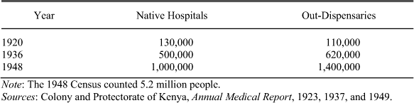
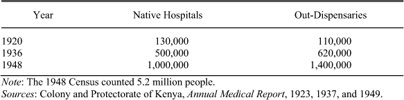
NUMBER OF TREATMENTS IN HEALTH FACILITIES IN KENYA

Note:

The 1948 Census counted 5.2 million people.

Sources:

Colony and Protectorate of Kenya, Annual Medical Report, 1923, 1937, and 1949.

What then caused the secular trend in Kenya? Several potential determinants can be put forward. As their influences are difficult to quantify, the explanations offered here are tentative.

The beneficial effects of Western medicine on health and living standards in Kenya are frequently overlooked. From the 1920s onwards, the health infrastructure expanded considerably. While 130,000 Kenyans were treated in “native hospitals” in 1920, the number of patients increased to 500,000 in 1936 and to one million in 1948.Footnote ⁶⁶ Additional 110,000, 620,000, and 1.4 million attendances were counted in out-dispensaries in 1923, 1936, and 1948 respectively (Table 5). By no means did the colonial system provide universal access, given the 1948 Census population of 5.2 million. Nevertheless, the rate of growth is extremely impressive.

Specific health strategies changed over the years. In the 1920s, for example, a campaign targeted tropical yaws, which was very common in rural areas. More than 700,000 Africans were treated and the incidence of the disease dropped markedly.Footnote ⁶⁷ Despite large-scale interventions like this, the colonial medical system placed an emphasis on preventive rather than curative care. Efforts included improvements in sanitation, health education, and vector management; specifically, the large-scale extermination of rats and bush clearances.Footnote ⁶⁸ In the early years, immunizations targeted plague and smallpox; later vaccines addressed tuberculosis and polio. In the 1950s modern antibiotics, particularly penicillin, became available, making treatments more effective overall.

The decentralized pattern of service delivery helped to extend medical coverage significantly. Several towns had hospitals and clinics; out-dispensaries staffed with skilled African personnel served rural areas, and members of the medical department regularly undertook “medical safaris” to remote communities. Geographically, medical services were indeed astonishingly well distributed (Figure 5). Nairobi had a favored position compared to other regions in terms of hospitals: in 1948, for example, 20 percent of hospital patients were treated in Nairobi, whereas her population share represented only 2 percent. On the other side of the scale is the lake region (Nyanza), where only 6 percent of all hospital patients were treated despite a population share of 34 percent. However, taking patients at out-dispensaries into account, provision of basic health care was roughly balanced—21 percent and 8 percent for Nyanza and Nairobi respectively. In addition, health care was financed by local taxes so that most services were provided without charging fees to Africans.Footnote ⁶⁹

Figure 5

MEDICAL TREATMENTS IN KENYA, 1936 AND 1948

Sources: Colony and Protectorate of Kenya, Annual Medical Report, 1937 and 1949.

The spread of Western medicine had an impact on mortality. Rough estimates of infant mortality rates in “native areas” in the 1920s ranged between 300 and 500 deaths per 1,000 live births, whereas infant mortality rates of 147.1 and 91.5 are reported for the 1950–1955 and 1970–1975 period respectively.Footnote ⁷⁰ William Brass and Carole L. Jolly confirmed the downward trend in death rates of children aged 0–5 years; applying indirect methods to Kenyan census data, they arrived at a child mortality rate of 270 for 1940, decreasing to 153 in 1974.Footnote ⁷¹

Summing up, progress in health care was substantial in the 1920–1970 period. The improvements in health almost certainly contributed to the positive trend in the nutritional status of Kenyans. However, the different experiences of ethnic groups suggest that health cannot be considered the only cause. The remarkable increase in stature of the Kikuyu is particularly striking and it is not clear that the Kikuyu benefited disproportionately from health services.

Improvements in nutrition must also be taken into account. Most Kenyans were dependent on agriculture for their livelihood—approximately 90 percent of the population in 1950.Footnote ⁷² Hence, the agricultural sector is of substantial importance. Unfortunately, quantitative aspects of agricultural production and trade are fuzzy. The output in subsistence agriculture was not documented. Moreover, African production found its way to domestic consumers mostly through informal marketing channels organized by African producers and traders, and Indian traders.Footnote ⁷³ It is only from the 1930s onwards that economic surveys and trade statistics provide a rough indication.

From the beginning of the century, a predominantly subsistence-based economy slowly changed to one based on commodity exchange. In the 1920s the commercialization of agriculture gained momentum.Footnote ⁷⁴ The portfolio of cash crops included wattle bark, sim sim, cotton, meat, and hides. Maize cultivation in particular, grown for the domestic market, expanded rapidly, benefiting both African producers and consumers. Shifting cultivation and long fallow periods made way to more intensive production. Both the area under cultivation and agricultural production increased.

Development was not uniform across regions. Using per capita sales of agricultural produce outside the district as a measure of peasant prosperity, Mosley found that Luo/Luhya and Kikuyu districts were on equal footing in 1929: sales of about 3 shillings per head were recorded for both regions.Footnote ⁷⁵ In 1945, however, the corresponding figures were 5 and 17 shillings (in 1929 prices), indicating that Kikuyu peasants were more prosperous. The diverging paths continued after World War II. As a response to the Mau Mau uprising, a land reform program was initiated in 1954 concentrating on the Highlands north of Nairobi, where the Kikuyu lived. The so-called Swynnerton Plan aimed at consolidating fragmented lands and providing for freehold titles. Restrictions on coffee cultivation were weakened. The reform brought additional incentives to intensification and cash-crop production. Productivity increased and cash revenues of African smallholders tripled during 1955–1964.Footnote ⁷⁶

The Kamba reserve had very different ecological and economic conditions and reports repeatedly point to agronomic deterioration from the 1930s onwards: soil erosion from overgrazing and intensive farming practices, low productivity, and underproduction.Footnote ⁷⁷ The Kamba lived on marginal lands susceptible to shortfalls in rain. From the early 1940s to the late 1950s, Kamba areas experienced a series of droughts and the population suffered from food shortages that could not be fully mitigated by migrant wage labor.Footnote ⁷⁸ However, in their study of the Machakos District, where the majority of the Kamba lived, Mary Tiffen, Michael Mortimore, and Francis Gichuki came to a different conclusion.Footnote ⁷⁹ According to them, from 1930 to 1990 environmental degradation was stopped and reversed, Boserup-style.Footnote ⁸⁰ They found that livestock numbers had decreased, but the value of crops per capita increased significantly. Still, for the time before 1960, production figures are unreliable and evidence remains scanty.Footnote ⁸¹

There are other factors to consider. Fiona MacKenzie, for example, argued that maize intensification weakened the position of women. Women provided the labor for maize production but had limited control over sales revenues.Footnote ⁸² Gender studies demonstrated that this can negatively affect child care, leading to lower nutrition and health for children, and hence to lower adult height.Footnote ⁸³ There are explanations beyond agricultural production. Increasing inequality, for example, put downward pressure on mean heights and one may indeed speculate that rising inequality affected Kikuyu heights as a whole. Additional factors include education, real wages, proximity to markets, and infrastructure. Ultimately, increasing heights reflected prosperity in a broad sense, whereas the different height trajectories of ethnic groups mirrored the economic inequalities at that time.

SUMMARY

The existing economic and social history literature is characterized by a pessimistic view of the colonial period, pointing to immiseration and downplaying aspects of modernization. The factual account, however, is essentially uncertain. Data is lacking and unreliable, and most measures fail to take into account differing economic systems and the transformations that took place in Kenya. Anthropometric indicators do not suffer from these shortcomings. Mean height of a population measures the outcome of nutrition and health consistently, and hence, indicates how well basic human needs are met.

Using height data from African army recruits and civilians this study found evidence for the following. First, large regional inequalities existed in late-nineteenth- and early-twentieth-century Kenya. Nutritional status was exceptionally poor in the central region, whereas conditions around Lake Victoria and in pastoral zones were much more favorable. Second, the nutritional status of cohorts born 20 years before and after colonization did not change significantly. Therefore, accounts of pre-colonial sufficiency, often implicitly made, cannot be maintained. Third, from 1920 onwards, secular improvements took place, which continued after independence for at least 15 years. Fourth, this development was particularly dynamic in the central region, so that inequality between ethnic groups declined over the course of the twentieth century.

My hypothesis is that climate-related diseases limited the height potential of ethnic groups indiscriminately and that the expanding health infrastructure, slightly favoring the central region and urban areas, improved the nutritional and health status of most Kenyans. Nutrition, I argue, is the factor that can explain the spatial pattern as well as the differences in mean height trajectories of ethnic groups, with nutritional status essentially following economic prosperity.

This study is the very first which has analyzed the Biological Standard of Living in an Eastern African colony. It is necessarily limited. The current data set cannot account for the ups and downs in the twentieth century. Short-term crises are important as their occurrences indicate failure to reduce exposure to risks. Also, not much can be said about inequality within ethnic groups. The increasing differentiation within the Kikuyu is a predominant theme, and an important one for understanding the Mau Mau uprising in the 1950s. Clearly, more research is needed. The potential of anthropometric techniques is not exhausted by this study, for historical records of body stature are an untapped source in African economic history. Heights of other social and occupational groups that allow for longer series and more covariates would be of great value in confirming the trends and providing a detailed account of social inequalities.

Acknowledging these limitations, one finding nonetheless stands out: colonial times were not as bad as commonly believed. In fact, the Kenya colony outperformed places like Mexico or India. This does not imply that colonialism was good. Colonial policies were a long way from maximizing the welfare of the indigenous population, and not all of the changes that occurred during the colonial era were the result of intention.