





1. Introduction
In tokamaks and stellarators, the large density and temperature gradients between the hot dense core and the cold dilute edge drive microinstabilities on the scale of the particles’ gyroradii. These microinstabilities give rise to turbulence which mixes the plasma, causing large heat fluxes limiting the energy confinement. The most virulent microinstabilities are typically on ion gyroradius scales, such as the ion temperature gradient (ITG) mode (Rudakov & Sagdeev Reference Rudakov and Sagdeev1961; Coppi, Rosenbluth & Sagdeev Reference Coppi, Rosenbluth and Sagdeev1967; Horton, Choi & Tang Reference Horton, Choi and Tang1981; Biglari, Diamond & Rosenbluth Reference Biglari, Diamond and Rosenbluth1989; Cowley, Kulsrud & Sudan Reference Cowley, Kulsrud and Sudan1991). When considering ion-scale microinstabilities, the passing electron response is generally assumed to be adiabatic. This assumption is motivated by the fast propagation rate of electrons
 $\omega _{{\scriptstyle \|}e} \sim v_{Te}/R$
parallel to the magnetic field. The typical frequency of ion-scale modes
 $\omega \sim v_{Ti}/R$
is comparatively slow, as
 $v_{Te}/v_{Ti} \sim (m_i/m_e)^{1/2} \gg 1$
. Here,
 $R$
is the major radius of the tokamak or stellarator, taken to be the typical system scale length, and
 $v_{T{s}} = (2 T_{s}/m_{s})^{1/2}$
is the thermal speed of particles of species
 $s$
with temperature
 $T_{s}$
and mass
 $m_{s}$
.
Notwithstanding the fast electron propagation, the non-adiabatic response of trapped electrons can become important even for ion-scale modes. Electrons trapped in regions of small magnetic field strength cannot respond adiabatically; this non-adiabatic trapped electron response can substantially modify the growth rate of ITG modes (see e.g. Dominski et al. Reference Dominski, Brunner, Görler, Jenko, Told and Villard2015) and give rise to trapped electron modes (TEMs) (Kadomtsev & Pogutse Reference Kadomtsev and Pogutse1967; Rosenbluth Reference Rosenbluth1968). Furthermore, the non-adiabatic response of passing electrons can also affect ion-scale modes. The non-adiabatic passing electron response typically leads to modes which extend far along the magnetic field line. Observations of such extended modes go back to early gyrokinetic simulations including kinetic electrons (Hallatschek & Dorland Reference Hallatschek and Dorland2005) and they have since been the object of various numerical studies (Dominski et al. Reference Dominski, Brunner, Görler, Jenko, Told and Villard2015; Belli, Candy & Waltz Reference Belli, Candy and Waltz2019; Ball, Brunner & A. Reference Ball, Brunner and C.J.2020; C. J. et al. Reference C. J., Brunner, McMillan, Ball, Dominski and Merlo2020, Reference C. J., Brunner and Ball2021).
By performing a multiscale expansion of the gyrokinetic system of equations in
 $m_e/m_i \ll 1$
, Hardman et al. (Reference Hardman, Parra, Chong, Adkins, Anastopoulos-Tzanis, Barnes, Dickinson, Parisi and Wilson2022) uncovered two types of electrostatic modes: the ‘small electron tail modes’ and the ‘dominant electron tail modes’, whose mode frequencies are determined by non-adiabatic ion physics and by non-adiabatic electron physics, respectively. In the expansion of Hardman et al. (Reference Hardman, Parra, Chong, Adkins, Anastopoulos-Tzanis, Barnes, Dickinson, Parisi and Wilson2022), the magnetic shear
 $\hat s$
, which describes the change in the field line pitch across flux surfaces, was assumed to be of order unity. For
 $\hat s \sim 1$
, the non-adiabatic ion response vanishes for
 $\theta \gg 1$
due to finite Larmor radius (FLR) effects. Here,
 $\theta$
is the poloidal angle and will be used throughout this work as a coordinate parallel to the magnetic field lines. Because of the ion FLR stabilisation, the ‘small electron tail modes’ are peaked at
 $\theta \sim 1$
and the non-adiabatic passing electron response only modifies the decay of the mode eigenfunction at
 $\theta \gg 1$
. In contrast, the eigenfunctions of the ‘dominant electron tail modes’ are extended in
 $\theta$
and the non-adiabatic ion response only causes a small change to the eigenfunction at
 $\theta \sim 1$
.
In this work, we present a theory of extended modes for small values of the magnetic shear
 $\hat s \sim (m_e/m_i)^{1/2}$
. With this ordering of
 $\hat s$
, the ion FLR effects become substantial only for large
 $\theta \sim (m_i/m_e)^{1/2}$
, the typical distance of electron propagation within a mode period
 $\omega ^{-1}\sim R/v_{Ti}$
. As a result, the mode frequency and eigenfunction are generally determined by non-adiabatic physics of both the electrons and the ions, unlike for the
 $\hat s \sim 1$
case. Notably, small values of the magnetic shear allow for a new type of microinstability. The new mode is prominent in the precise quasisymmetric stellarators of Landreman & Paul (Reference Landreman and Paul2022) (see § 5). The mode is also a salient feature of tokamak simulations at small magnetic shear, where it was called a ‘
 $k_z \approx 0$
’ toroidal ITG mode (Volčokas et al. Reference Volčokas, Ball and Brunner2023, Reference Volčokas, Ball and Brunner2024b
). Henceforth, we call the new mode a geodesic extended mode (GEM), due to its connection with geodesic acoustic mode physics (see § 4).
In figure 1, we show representative gyrokinetic simulations exhibiting GEMs. The GEMs are indeed very extended compared with modes of a larger magnetic shear case, see figure 1(b). Furthermore, compared with the localised modes found at larger magnetic shear
 $\hat s \approx 0.8$
, the GEMs oscillate rapidly in time and have a larger growth rate at small binormal wavenumbers.
(a) Complex frequency and (b) eigenmode structure for
 $k_y \rho _i = 0.1$
at small and large magnetic shear,
 $\hat s =0.01$
and
 $\hat s = 0.8$
. The data are obtained from gyrokinetic simulations using the stella code (Barnes, Parra & Landreman Reference Barnes, Parra and Landreman2019) for a tokamak with circular cross-section. The safety factor is
 $q=2.38$
, the electron-to-ion mass ratio is
 $m_e/m_i = 1/1836$
and a pure ion temperature gradient drive is considered,
 $a/L_{Ti}=4$
and
 $a/L_{Te}=a/L_n = 0$
, where
 $a$
is the plasma minor radius. All other parameters are identical to those presented in § 3.1.

Figure 1. Long description
The image contains two panels with graphs. Panel A shows two line graphs. The top graph plots the growth rate (ωiR/vTi) against the binormal wavenumber (kyρi) for two different values of magnetic shear (ŝ = 0.01 and ŝ = 0.80). The bottom graph plots the real frequency (ωrR/vTi) against the binormal wavenumber (kyρi) for the same values of magnetic shear. Both graphs use a logarithmic scale for the y-axis and a linear scale for the x-axis. The red line represents ŝ = 0.01, and the blue line represents ŝ = 0.80. Panel B shows a line graph of the potential fluctuation ballooning structure (|δφ̂|) along the magnetic field for kyρi = 0.1. The x-axis represents the angle (θ) in radians, and the y-axis represents the potential fluctuation (|δφ̂|). The red line represents ŝ = 0.01, and the blue line represents ŝ = 0.80. The graph shows two peaks and a dip in the middle, indicating the structure of the potential fluctuation.
The effect of low magnetic shear values on non-adiabatic passing electron physics has been studied in a series of recent papers by Volčokas et al. (Reference Volčokas, Ball and Brunner2023, Reference Volčokas, Ball and Brunner2024a , Reference Volčokas, Ball and Brunnerb , Reference Volčokas, Ball, Di Giannatale and Brunner2025). Small values of magnetic shear are a common occurrence in stellarator magnetic fields, for example, in stellarators optimised for quasisymmetry (Landreman & Paul Reference Landreman and Paul2022; Nies et al. Reference Nies, Paul, Panici, Hudson and Bhattacharjee2024; Buller et al. Reference Buller, Landreman, Kappel and Gaur2025). In tokamaks, small magnetic shear values are especially relevant for reverse-shear operating scenarios, where the safety factor has a minimum away from the magnetic axis (in common tokamak operating scenarios, the safety factor monotonically increases from the core to the edge). In some reverse-shear discharges, large internal transport barriers were observed (see e.g. Levinton et al. Reference Levinton1995; Strait et al. Reference Strait1995; Eriksson et al. Reference Eriksson2002), with greatly improved plasma confinement. It has been suggested by Volčokas et al. (Reference Volčokas, Ball, Di Giannatale and Brunner2025) that these transport barriers arise due to the flattening of the safety factor profile caused by the self-interaction of extended modes, further motivating the study of the GEMs. We note that extended modes (though typically less extended than the modes presented in this paper) were also previously observed in linear gyrokinetic simulations at low magnetic shear for electrostatic instabilities in tokamaks and stellarators (Zocco et al. Reference Zocco, Xanthopoulos, Doerk, Connor and Helander2018), and for electromagnetic instabilities in tokamaks (Mulholland et al. Reference Mulholland, Zocco, Morren, Aleynikova, Pueschel, Proll and Terry2025).
This paper is structured as follows. We first present the theory of extended modes at small magnetic shear in § 2. The theory is then validated against gyrokinetic simulations in § 3, which will also reveal the parametric dependences of the GEMs. We then elucidate the physics of the GEMs in § 4. In § 5, we show that GEMs are important to understand linear and nonlinear gyrokinetic simulations in stellarators by considering the precise quasi-axisymmetric stellarator of Landreman & Paul (Reference Landreman and Paul2022). Finally, we conclude and discuss our results in § 6.
2. Theory of extended modes
In § 2.1, we review the theory of gyrokinetics used to describe microinstabilities in tokamak and stellarator plasmas. We introduce the multiscale expansion of the gyrokinetic equation along the field line in § 2.2. We derive the ion and electron contributions to quasineutrality in a particular convenient limit in §§ 2.3 and 2.4, respectively. These allow us to derive the dispersion relation for extended tail modes in § 2.5. In § 2.6, we consider a subsidiary limit of slow electron propagation over the scale of the mode and finally, in § 2.7, we consider a simplified dispersion relation assuming fluid ions and negligible electron propagation.
2.1. Linear gyrokinetics in tokamaks and stellarators
We consider a strongly magnetised plasma, i.e. the gyroradius
 $\rho _{s} = v_{T{s}}/\varOmega _{s}$
is much smaller than the system size (
 $\rho _{s} \ll R$
), with
 $\varOmega _{s} = Z_{s} e B/m_{s}$
the Larmor frequency,
 $Z_{s} e$
the particle charge,
 $e$
the proton charge and
 $B$
the magnetic field strength. The fast gyromotion of particles may then be averaged over to derive gyrokinetics (Catto Reference Catto1978; Frieman & Chen Reference Frieman and Chen1982), a kinetic theory describing the motion of rings of charge. We consider
 $\delta f$
-gyrokinetics: for each species, the particle distribution function
 $f_{s}$
may be decomposed as
 $f_{s} = F_{M{s}} + \delta f_{s}$
, where the fluctuating distribution function
 $\delta f_{s} \sim (\rho _{s}/R) F_{M{s}}$
is small compared with the background Maxwellian
 \begin{align} F_{M{s}} = \frac {n_{s}}{\pi ^{3/2} v_{T{s}}^3} \exp \left ( - \frac {v^2}{v_{T{s}}^2} \right ), \end{align}
with
 $n_{s}$
the background density and
 $v$
the particle speed. The spatial derivatives of the fluctuating distribution function are ordered as
 \begin{align} |\boldsymbol{\hat {b}} \boldsymbol{\cdot }\boldsymbol{\nabla }\ln \delta f_{s}| \sim 1/R, \qquad |\boldsymbol{\hat {b}} \times \boldsymbol{\nabla }\ln \delta f_{s}| \sim 1/\rho _{s}, \end{align}
corresponding to anisotropic turbulent eddies that are elongated along the magnetic field, but are narrow in the direction perpendicular to it. Here,
 $\boldsymbol{\hat {b}} = \boldsymbol{B}/B$
is the unit magnetic field vector. Finally, the derivatives in velocity space and with respect to time are ordered as
 \begin{align} |\partial _{\boldsymbol{v}} \ln \delta f_{s}| \sim 1/v_{T{s}}, \qquad |\partial _t \ln \delta f_{s}| \sim v_{T{s}}/R. \end{align}
It is convenient to express the gyrokinetic equation in terms of the non-adiabatic contribution to the distribution function
 $h_{s}$
, which satisfies
 \begin{align} \delta f_{s}(\boldsymbol{r}, \sigma , \varepsilon , \mu , \vartheta ,t) = h_{s}(\boldsymbol{R}, \sigma , \varepsilon , \mu , t) - \frac {Z_{s} e \delta \varphi (\boldsymbol{r})}{T_{s}} F_{M{s}}, \end{align}
with
 $\delta \varphi$
the fluctuating electrostatic potential. Here, we have defined the sign of the parallel velocity
 $\sigma =v_{\scriptstyle \|} / |v_{\scriptstyle \|}|$
with
 $v_{\scriptstyle \|}=\boldsymbol{v}\boldsymbol{\cdot }\boldsymbol{\hat {b}}$
, the particle energy
 $\varepsilon =m_{s} v^2/2$
, the magnetic moment
 $\mu = m_{s} v_\perp ^2/(2B)$
, the gyrophase
 $\vartheta$
measuring the angle between
 $\boldsymbol{v}_\perp = \boldsymbol{v}-v_{\scriptstyle \|}\boldsymbol{\hat {b}}$
and an arbitrarily defined coordinate axis perpendicular to the magnetic field, and finally the guiding centre position
 \begin{align} \boldsymbol{R} = \boldsymbol{r} - \frac {\boldsymbol{\hat {b}}\times \boldsymbol{v}}{\varOmega _{s}}, \end{align}
which is shifted from the real space position
 $\boldsymbol{r}$
by the gyroradius vector. We note that the non-adiabatic piece
 $h_s$
does not depend on the gyrophase
 $\vartheta$
.
We consider the linearised, electrostatic, collisionless and low-flow limit of the gyrokinetic equation, given by
 \begin{align} \frac {\partial h_{{s}}}{\partial t} + \big(v_{\scriptstyle \|} \boldsymbol{\hat {b}} + \tilde {\boldsymbol{v}}_{Ms}\big) \boldsymbol{\cdot }\frac {\partial h_{{s}}}{\partial \boldsymbol{R}} + \langle \boldsymbol{v}_E \rangle _{\boldsymbol{R}}\boldsymbol{\cdot }\frac {\partial F_{M{s}}}{\partial \boldsymbol{R}} = \frac {Z_{s} e}{T_{s}} \frac {\partial \left \langle \delta \varphi \right \rangle _{\boldsymbol{R}}}{\partial t} F_{M{s}}, \end{align}
where
 $\left \langle \right \rangle _{\boldsymbol{R}}$
is a gyro-average (average over the gyrophase
 $\vartheta$
) at fixed guiding centre position
 $\boldsymbol{R}$
. Here, we defined the fluctuating
 $\boldsymbol{E}\times \boldsymbol{B}$
drift velocity
 \begin{align} \boldsymbol{v}_E = \frac {\boldsymbol{\hat {b}}\times \boldsymbol{\nabla }\delta \varphi }{B}, \end{align}
and the magnetic drift velocity
 \begin{align} \tilde {\boldsymbol{v}}_{Ms} = \frac {\boldsymbol{\hat {b}}}{\varOmega _{s}} \times \left ( v_{\scriptstyle \|}^2 \boldsymbol{\hat {b}}\boldsymbol{\cdot }\boldsymbol{\nabla }\boldsymbol{\hat {b}} + \frac {v_\perp ^2}{2}\boldsymbol{\nabla }\ln B \right ), \end{align}
which is the combination of the curvature and
 $\boldsymbol{\nabla }B$
drifts.
The fluctuating electrostatic potential
 $\delta \varphi$
entering the gyrokinetic equation (2.6) is obtained self-consistently from the quasineutrality equation
 \begin{align} 0 = \sum _{s} Z_{s} \int \mathrm{d}^3 v\, \delta f_{s} = - \sum _{s} \frac {Z_{s}^2 e n_{s}}{T_{s}} \delta \varphi + \sum _{s} Z_{s} \int \mathrm{d}^3 v\, \langle h_{{s}}\rangle _{\boldsymbol{r}}, \end{align}
where
 $\langle \rangle _{\boldsymbol{r}}$
denotes a gyro-average at fixed real space position
 $\boldsymbol{r}$
.
In a tokamak or stellarator, it is convenient to use the coordinate system
 $(\psi , {{\alpha }}, \theta )$
, where
 $\psi$
is the poloidal flux labelling flux surfaces and
 ${{\alpha }} = \zeta - q\theta + \nu (\theta ,\zeta )$
is a field line label defined such that
 $\boldsymbol{B}=\boldsymbol{\nabla }\psi \times \boldsymbol{\nabla }{{\alpha }}$
. Here,
 $\nu$
is a single-valued function of the toroidal and poloidal angles
 $\zeta$
and
 $\theta$
, and
 $q=q(\psi )$
is the safety factor measuring the average pitch of magnetic field lines on a flux surface.
We consider a narrow flux tube centred on the flux surface
 $\psi _0$
and field line
 ${\alpha _{0}}$
. The flux tube domain is parametrised in the perpendicular directions by
 \begin{align} x = (\psi -\psi _0) \frac {\mathrm{d} x}{\mathrm{d} \psi }, \qquad y = ({{\alpha }}-{{\alpha _{0}}}) \frac {\mathrm{d} y}{\mathrm{d} {{\alpha }}}, \end{align}
with the radial coordinate
 $x$
labelling flux surfaces and the binormal coordinate
 $y$
labelling field lines on a flux surface. The constants
 $\mathrm{d} x/\mathrm{d}\psi$
and
 $\mathrm{d}y/\mathrm{d}{{\alpha }}$
are arbitrary, and are chosen differently in different formulations and codes.
Because the flux tube is narrow in the direction perpendicular to
 $\boldsymbol{B}$
compared with the system scale length, statistical periodicity of the fluctuations may be invoked to justify the use of periodic boundary conditions in the directions perpendicular to
 $\boldsymbol{B}$
. We may therefore consider the fluctuations in Fourier space, parametrised by a binormal wavenumber
 $k_y$
and radial wavenumber
 $k_x$
. We also consider Fourier eigenmodes in time, allowing us to express the distribution function and fluctuating electrostatic potential as
 \begin{align} h_s(t, X, Y, \theta , \varepsilon , \mu , \sigma ) & = \sum _{k_x, k_y, \omega } \hat h_s(\omega , k_x, k_y, \theta , \varepsilon , \mu , \sigma )e^{-i\omega t+ik_x X+ik_y Y},\\[-10pt]\nonumber \end{align}
 \begin{align} \delta \varphi (t, x, y, \theta ) & = \sum _{k_x, k_y, \omega } \delta \hat \varphi (\omega , \theta , k_x, k_y)e^{-i\omega t+ik_x x+ik_y y}, \end{align}
where
 $X$
and
 $Y$
are the radial and binormal coordinates of the guiding centre.
It will prove convenient to express the radial wavenumber through the quantity
 \begin{align} \theta _0 = \frac {k_x}{k_y} \left (\frac {\mathrm{d} q}{\mathrm{d} x} \frac {\mathrm{d} y}{\mathrm{d} {{\alpha }}} \right )^{-1}. \end{align}
The perpendicular wavevector may then be written as
 \begin{align} \boldsymbol{k}_\perp & = k_x \boldsymbol{\nabla }x + k_y \boldsymbol{\nabla }y \nonumber \\ & = k_y \frac {\mathrm{d} y}{\mathrm{d} {{\alpha }}} \left ( \boldsymbol{\nabla }\zeta \left (1 + \partial _\zeta \nu \right ) + \boldsymbol{\nabla }\theta \left ( - q + \partial _\theta \nu \right ) + \boldsymbol{\nabla }x \frac {\mathrm{d} q}{\mathrm{d} x} \left ( \theta _0-\theta \right ) \right ), \end{align}
where the last term captures the secular increase in
 $\theta$
due to magnetic shear
 \begin{align} \hat s = \frac {\mathrm{d}\ln q}{\mathrm{d}\ln \psi } = \frac {\psi _0}{q(\psi _0)} \frac {\mathrm{d}x}{\mathrm{d}\psi } \frac {\mathrm{d} q}{\mathrm{d} x}. \end{align}
In Fourier space, the linearised GK equation (2.6) is given by
 \begin{align} (\omega - \tilde {\omega }_{M{s}}) \hat h_{s} + i v_{\scriptstyle \|} \boldsymbol{\hat {b}}\boldsymbol{\cdot }\boldsymbol{\nabla }\theta \frac {\partial \hat h_{s}}{\partial \theta } = (\omega - \tilde \omega _{*{s}}) J_{0{s}} F_{M{s}} \frac {Z_{s} e \delta \hat \varphi }{T_{s}}, \end{align}
and the quasineutrality equation (2.9) becomes
 \begin{align} 0 = \sum _{s} Z_{s} \delta \hat n_{s} = - \sum _{s} \frac {Z_{s}^2 e n_{s}}{T_{s}} \delta \hat \varphi + \sum _{s} Z_{s} \int \mathrm{d}^3 v\, J_{0{s}}\hat h_{{s}}. \end{align}
Equation (2.16) is an ordinary differential equation in
 $\theta$
, with
 $\theta \in (-\infty , \infty )$
. For passing particles, we assume that there is no inflow of particles from infinity, i.e.
 \begin{align} \lim _{\theta \rightarrow -\sigma \infty }\hat h_{s}^{\mathrm{p}}(\theta ,\sigma ) = 0. \end{align}
For trapped particles, the distribution function must be independent of
 $\sigma$
at the bounce points
 $\theta _b^{\pm }$
, i.e.
 \begin{align} \hat h_{s}^{\mathrm{t}}\big(\theta _b^\pm ,\sigma =1\big) = \hat h_{s}^{\mathrm{t}}\big(\theta _b^\pm ,\sigma =-1\big). \end{align}
In (2.16), the magnetic drift frequency is defined as
 \begin{align} \tilde {\omega }_{M{s}} = \boldsymbol{k}_\perp \boldsymbol{\cdot }\tilde {\boldsymbol{v}}_{M{s}}, \end{align}
and the diamagnetic frequency is given by
 \begin{align} \tilde \omega _{*{s}} & = \omega _{*{s}} + \omega _{*{s}}^T \left ( \frac {v^2}{v_{T{s}}^2} - \frac {3}{2} \right ) \nonumber \\[5pt] & = -k_y \frac {\mathrm{d} y}{\mathrm{d} {{\alpha }}} \frac {T_{s}}{Z_{s} e} \left ( \frac {\mathrm{d} \ln n_{s}}{\mathrm{d} \psi } + \frac {\mathrm{d} \ln T_{s}}{\mathrm{d} \psi } \left ( \frac {v^2}{v_{T{s}}^2} - \frac {3}{2} \right ) \right ), \end{align}
which implicitly defines
 $\omega _{*{s}}$
and
 $\omega _{*{s}}^T$
. Finite Larmor radius effects are captured by the Bessel functions of the first kind
 \begin{align} J_{0{s}} = J_0 \left ( \frac {k_\perp v_\perp }{\varOmega _{s}} \right ). \end{align}
2.2. Ordering and multiscale expansion
As discussed previously, the modes we seek to describe become very extended along the magnetic field as the magnetic shear is reduced. However, these modes will also have some variation over smaller scales (
 $\theta \sim 1$
) due to the variation of the magnetic geometry, which enters
 $\tilde \omega _{Ms}$
and
 $J_{0s}$
. To capture both of these behaviours, we follow in the footsteps of Hardman et al. (Reference Hardman, Parra, Chong, Adkins, Anastopoulos-Tzanis, Barnes, Dickinson, Parisi and Wilson2022) and consider a multiscale expansion in
 $\theta$
of the distribution function,
 $\hat h_{s}(\theta ) \rightarrow \hat h_{s}(\theta _s, \theta _f)$
. Here,
 $\theta _f$
captures the fast variation of geometric quantities, typically over a single poloidal turn, while
 $\theta _s$
captures the slower variation due to the magnetic shear.
We use the small electron-to-ion mass ratio to define the expansion parameter
 \begin{align} \epsilon = \sqrt {m_e/m_i} \ll 1 \end{align}
and we order the magnetic shear to be small in
 $\epsilon$
, i.e.
 \begin{align} \hat s \sim \epsilon . \end{align}
To leading order in
 $\epsilon$
, we may approximate the perpendicular wavenumber vector (2.14) as
 \begin{align} \boldsymbol{k}_\perp = k_y \frac {\mathrm{d} y}{\mathrm{d} {{\alpha }}} \left ( \boldsymbol{\nabla }\zeta \left (1 + \partial _\zeta \nu \right ) + \boldsymbol{\nabla }\theta \left ( - q + \partial _\theta \nu \right ) - \boldsymbol{\nabla }x \frac {\mathrm{d} q}{\mathrm{d} x} \theta _s \right ), \end{align}
where the secular variation due to the magnetic shear is captured through
 $\theta _s$
only, and
 $\boldsymbol{\nabla }\zeta$
,
 $\boldsymbol{\nabla }\theta$
,
 $\partial _\zeta \nu$
,
 $\partial _\theta \nu$
and
 $\boldsymbol{\nabla }x$
are functions of
 $\theta _f$
only. We also neglected the contribution from
 $\theta _0$
to the secular term in (2.14), i.e. we assumed
 $\theta _s \gg \theta _0 \sim 1$
. This may be justified rigorously in a tokamak, where
 $\theta _0 \in [0,2\pi )$
without loss of generality.
The terms in the gyrokinetic equation (2.16) for ions and electrons are ordered as
 \begin{align} \epsilon \, v_{Te} \boldsymbol{\hat {b}} \boldsymbol{\cdot }\boldsymbol{\nabla }\theta \frac {\partial \ln \hat h_e}{\partial \theta _f} \sim v_{Te} \boldsymbol{\hat {b}} \boldsymbol{\cdot }\boldsymbol{\nabla }\theta \frac {\partial \ln \hat h_e}{\partial \theta _s} \sim \tilde \omega _{*e} \sim \tilde \omega _{Me} \sim v_{Ti} \boldsymbol{\hat {b}} \boldsymbol{\cdot }\boldsymbol{\nabla }\theta \frac {\partial \ln \hat h_i}{\partial \theta _f} \sim \tilde \omega _{*i} \sim \tilde \omega _{Mi} \sim \omega . \end{align}
The electrons propagate quickly over a distance
 $\theta _f$
, while their propagation speed over a distance
 $\theta _s$
is maximally ordered with the mode frequency, the magnetic drift frequencies, the diamagnetic frequencies, and the ion propagation speed over
 $\theta _f$
.
In what follows, we consider a single ion species for ease of notation, though the theory may easily be generalised to multiple species. We study ion-scale modes with
 $k_\perp \rho _e \ll k_\perp \rho _i \sim 1$
. We therefore neglect electron FLR effects, such that
 $J_{0e}=1$
.
2.3. Local ion response
With the ordering equation (2.26), the gyrokinetic equation (2.16) for the ions is given by
 \begin{align} (\omega - \tilde {\omega }_{Mi}) \hat h_i + i v_{\scriptstyle \|} \boldsymbol{\hat {b}}\boldsymbol{\cdot }\boldsymbol{\nabla }\theta \frac {\partial \hat h_i}{\partial \theta _f} = (\omega - \tilde \omega _{*i}) J_{0i} F_{Mi} \frac {Z_i e \delta \hat \varphi }{T_i}. \end{align}
To make further progress, we neglect the ion parallel streaming term. This approximation is often appropriate for the geodesic extended modes, which oscillate rapidly with frequency
 $\omega \sim v_{Ti}/R$
, even for small
 $k_y \rho _i$
(see figure 1a
). The ion parallel streaming may be neglected when the connection length is sufficiently long; we discuss this approximation in § 4.4. Neglecting the ion parallel streaming, the ion gyrokinetic equation (2.27) simplifies to an algebraic equation, which may be rearranged to obtain
 \begin{align} \hat h_i = \frac {\omega - \tilde \omega _{*i}}{\omega - \tilde {\omega }_{Mi}} J_{0i} F_{Mi} \frac {Z_i e \delta \hat \varphi }{T_i}. \end{align}
The ion density fluctuations may therefore be written as
 \begin{align} \frac {\delta \hat n_i}{n_i} = -\frac {Z_i e \delta \hat \varphi }{T_i} + \frac {1}{n_i}\int \mathrm{d}^3 v\, J_{0i}\hat h_{i} = -\frac {Z_i e \delta \hat \varphi }{T_i} (1-\mathcal{M}_i), \end{align}
where we defined the ion response function
 \begin{align} \mathcal{M}_i = \frac {1}{n_i}\int \mathrm{d}^3 v\, \frac {\omega - \tilde \omega _{*i}}{\omega - \tilde {\omega }_{Mi}} J_{0i}^2 F_{Mi}, \end{align}
which depends on both
 $\theta _f$
and
 $\theta _s$
through the Bessel functions and the magnetic drift frequency.
To numerically evaluate
 $\mathcal{M}_i$
, it is convenient to express the velocity integral as a one-dimensional integral (Terry, Anderson & Horton Reference Terry, Anderson and Horton1982). We consider unstable modes (Im
 $(\omega )\gt 0$
), such that the resonant denominator in (2.30) may be written as
 \begin{align} \frac {1}{ \omega - \tilde {\omega }_{Mi}} = -i \int _0^\infty \mathrm{d}\varLambda \, \exp [ i \varLambda (\omega -\tilde {\omega }_{Mi}) ]. \end{align}
The ion response function (2.30) may then be reduced to (see also Biglari et al. Reference Biglari, Diamond and Rosenbluth1989; Zocco et al. Reference Zocco, Xanthopoulos, Doerk, Connor and Helander2018; Parisi et al. Reference Parisi2020)
 \begin{align} \mathcal{M}_i & = -i \int _0^\infty \mathrm{d}\varLambda \frac {e^{i\varLambda \omega }}{\sqrt {1+i\varLambda \omega _{\kappa ,i}}} \frac {1}{1+i \varLambda \omega _{\boldsymbol{\nabla }B,i} /2} \Bigg \{ \tilde b_i ( \varGamma _0(\tilde b_i) - \varGamma _1(\tilde b_i) ) \frac {\omega _{*i}^T}{1 + i \varLambda \omega _{\boldsymbol{\nabla }B,i}/2} \nonumber \\[5pt] & \quad + \varGamma _0(\tilde b_i) \left ( \omega - \omega _{*i} - \omega _{*i}^T \left ( \frac {1/2}{1+i \varLambda \omega _{\kappa ,i}} + \frac {1}{1+i\varLambda \omega _{\boldsymbol{\nabla }B,i}/2} - \frac {3}{2} \right ) \right ) \Bigg \}, \end{align}
where we have defined the curvature drift frequency
 \begin{align} \omega _{\kappa ,i} = \frac {v_{Ti}^2}{\varOmega _i} \boldsymbol{k}_\perp \boldsymbol{\cdot }\boldsymbol{\hat {b}} \times (\boldsymbol{\hat {b}}\boldsymbol{\cdot }\boldsymbol{\nabla }\boldsymbol{\hat {b}}), \end{align}
the
 $\boldsymbol{\nabla }B$
drift frequency
 \begin{align} \omega _{\boldsymbol{\nabla }B,i} = \frac {v_{Ti}^2}{\varOmega _i}\boldsymbol{k}_\perp \boldsymbol{\cdot }\boldsymbol{\hat {b}} \times \boldsymbol{\nabla }\ln B \end{align}
and the quantity
 \begin{align} \tilde b_i = \frac {k_\perp ^2 \rho _i^2}{2} \frac {1}{1 + i \varLambda \omega _{\boldsymbol{\nabla }B,i}/2}, \end{align}
which sets the strength of ion FLR effects. These enter in (2.32) through the functions
 $\varGamma _n(\tilde b_i) = I_n(\tilde b_i) e^{-\tilde b_i}$
, where
 $I_n$
is the modified Bessel function of the first kind.
The integral over
 $\varLambda$
in (2.32) is well behaved as long as Re
 $(\varLambda ) \rightarrow +\infty$
and Im
 $(\omega ) \gt 0$
, such that the complex exponential
 $e^{i\varLambda \omega }$
decays. Numerically, we find it sufficient to carry out the integration along the positive real axis of
 $\varLambda$
, though other integration paths may also be considered (see e.g. Parisi et al. Reference Parisi2020).
2.4. Electron propagator
The electron distribution function is expanded in the parameter
 $\epsilon$
as
 \begin{align} \hat h_e = \hat h_{e,(0)} + \hat h_{e,(1)} + \ldots , \end{align}
where
 $\hat h_{e,(n)} \sim \epsilon ^n \hat h_e$
. With the ordering (2.26), the electron gyrokinetic equation is given to leading order by
 \begin{align} i v_{\scriptstyle \|} \boldsymbol{\hat {b}}\boldsymbol{\cdot }\boldsymbol{\nabla }\theta \frac {\partial \hat h_{e,(0)}}{\partial \theta _f} = 0, \end{align}
and to next order by
 \begin{align} (\omega - \tilde {\omega }_{M e}) \hat h_{e,(0)} + i v_{\scriptstyle \|} \boldsymbol{\hat {b}}\boldsymbol{\cdot }\boldsymbol{\nabla }\theta \frac {\partial \hat h_{e,(0)}}{\partial \theta _s} + i v_{\scriptstyle \|} \boldsymbol{\hat {b}}\boldsymbol{\cdot }\boldsymbol{\nabla }\theta \frac {\partial \hat h_{e,(1)}}{\partial \theta _f} = -(\omega - \tilde \omega _{*e}) F_{Me} \frac {e \delta \hat \varphi }{T_e}. \end{align}
We now define the transit average over the fast coordinate
 $\theta _f$
,
 \begin{align} \langle A \rangle _{\tau _f} = \begin{cases} \left ( \displaystyle\int _{\theta _f^-}^{\theta _f^+} \mathrm{d}\theta _f \dfrac {A}{v_{\scriptscriptstyle \|} \boldsymbol{\hat {b}}\boldsymbol{\cdot }\boldsymbol{\nabla }\theta } \right ) \Big / \left ( \displaystyle\int _{\theta _f^-}^{\theta _f^+} \mathrm{d}\theta _f \dfrac {1}{v_{\scriptscriptstyle \|} \boldsymbol{\hat {b}}\boldsymbol{\cdot }\boldsymbol{\nabla }\theta } \right ) \qquad & (\text{passing}),\\[16pt] \left (\sum _\sigma \displaystyle\int _{\theta _b^-}^{\theta _b^+} \mathrm{d}\theta _f \dfrac {A}{|v_{\scriptscriptstyle \|}| \boldsymbol{\hat {b}}\boldsymbol{\cdot }\boldsymbol{\nabla }\theta } \right ) \Big / \left (2 \displaystyle\int _{\theta _b^-}^{\theta _b^+} \mathrm{d}\theta _f \dfrac {1}{|v_{\scriptscriptstyle \|}| \boldsymbol{\hat {b}}\boldsymbol{\cdot }\boldsymbol{\nabla }\theta } \right ) \qquad & (\text{trapped}). \end{cases} \end{align}
Here,
 $\theta _b^\pm$
are the bounce points of trapped particles. We proceed to discuss the limits of integration
 $\theta _f^\pm$
for the passing particle transit average over the fast coordinate. We assume the existence of a periodicity length in the fast variable
 $\theta _f$
given by
 $\theta _f^+ - \theta _f^-$
. Thus, the passing electron distribution function is assumed to satisfy
 \begin{align} \hat h_e^{\mathrm{p}}\big(\theta _f = \theta _f^-\big) = \hat h_e^{\mathrm{p}}\big(\theta _f =\theta _f^+\big). \end{align}
This assumption is justified in tokamaks, where
 $\theta _f^\pm = \pm \pi$
as all geometric quantities are periodic in
 $\theta$
, and on rational flux surfaces in stellarators, where
 $\theta _f^\pm = \pm N\pi$
, as geometric quantities are periodic after
 $N$
poloidal turns if
 $q = M/N$
with
 $M,N\in \mathbb{N}$
. On an irrational flux surface in a stellarator, finding
 $\theta _f^\pm$
such that (2.40) is satisfied requires the flux tube to have sufficiently sampled the geometry of the flux surface.
From (2.37), the leading order electron distribution function satisfies
 \begin{align} \hat h_{e,(0)} = \big\langle \hat h_{e,(0)} \big\rangle _{\tau _f} \end{align}
and is determined as a solvability condition of (2.38), whose transit average over the fast coordinate is given by
 \begin{align} (\omega - \langle \tilde {\omega }_{M e} \rangle _{\tau _f}) \hat h_{e,(0)} + i \big\langle v_{\scriptstyle \|} \boldsymbol{\hat {b}}\boldsymbol{\cdot }\boldsymbol{\nabla }\theta \big\rangle _{\tau _f} \frac {\partial \hat h_{e,(0)}}{\partial \theta _s} = -(\omega - \tilde \omega _{*e}) F_{Me} \frac {e \langle \delta \hat \varphi \rangle _{\tau _f}}{T_e}. \end{align}
As trapped particles are localised in magnetic field wells, they cannot sample the slow variation in
 $\theta _s$
. Indeed,
 $\langle v_{\scriptstyle \|} \boldsymbol{\hat {b}}\boldsymbol{\cdot }\boldsymbol{\nabla }\theta \rangle _{\tau _f} = 0$
for trapped particles and the trapped electron distribution
 $\hat h_{e,(0)}^{\mathrm{t}}$
is therefore given by
 \begin{align} \hat h_{e,(0)}^{\mathrm{t}} = -\frac {\omega - \tilde \omega _{*e}}{\omega - \langle \tilde {\omega }_{M e} \rangle _{\tau _f}} F_{Me} \frac {e \langle \delta \hat \varphi \rangle _{\tau _f}}{T_e}. \end{align}
To determine the passing electron distribution function
 $h_{e,(0)}^{\mathrm{p}}$
, we first define
 \begin{align} \phi _e(\theta _s) = \frac {\omega - \langle \tilde {\omega }_{M e} \rangle _{\tau _f}}{\big\langle v_{\scriptstyle \|} \boldsymbol{\hat {b}}\boldsymbol{\cdot }\boldsymbol{\nabla }\theta \big\rangle _{\tau _f}} \end{align}
and
 \begin{align} H_e = \hat h_{e,(0)}^{\mathrm{p}} \exp \left (-i \int ^{\theta _s}\mathrm{d}\theta _s'\,\phi _e(\theta _s')\right ). \end{align}
Equation (2.42) for passing particles may then be written as
 \begin{align} i \big\langle v_{\scriptstyle \|} \boldsymbol{\hat {b}}\boldsymbol{\cdot }\boldsymbol{\nabla }\theta \big\rangle _{\tau _f} \frac {\partial H_e}{\partial \theta _s} = -(\omega - \tilde \omega _{*e}) F_{Me} \frac {e \langle \delta \hat \varphi \rangle _{\tau _f}}{T_e} \exp \left (-i \int ^{\theta _s}\mathrm{d}\theta _s'\,\phi _e(\theta _s')\right ). \end{align}
Integrating from infinity and using the boundary condition (2.18), the leading order electron distribution function is derived to be
 \begin{align} \hat h_{e,(0)}^{\mathrm{p}}(\theta _s) = i \frac {\omega - \tilde \omega _{*e}}{\big\langle v_{\scriptstyle \|} \boldsymbol{\hat {b}}\boldsymbol{\cdot }\boldsymbol{\nabla }\theta \big\rangle _{\tau _f}} F_{Me} \int _{-\sigma \infty }^{\theta _s} \mathrm{d}\theta _s' \frac {e \langle \delta \hat \varphi \rangle _{\tau _f}(\theta _s')}{T_e} \exp \left (i \int ^{\theta _s}_{\theta _s'}\mathrm{d}\theta _s''\,\phi _e(\theta _s'')\right ). \end{align}
To make further progress, we now make two simplifying assumptions. First, we consider a large aspect ratio configuration, i.e. the variation of
 $B$
and
 $v_{\scriptstyle \|}$
in
 $\theta$
are assumed to be negligible. Therefore, the number of trapped particles is negligibly small and transit averages over the fast coordinate (2.39) simplify to averages over
 $\theta _f$
,
 \begin{align} \langle A \rangle _{\tau _f} \rightarrow \langle A \rangle _{\theta _f} = \left ( \int _{\theta _f^-}^{\theta _f^+} \mathrm{d}\theta _f \frac {A}{\boldsymbol{\hat {b}}\boldsymbol{\cdot }\boldsymbol{\nabla }\theta } \right ) \Bigg / \left ( \int _{\theta _f^-}^{\theta _f^+} \mathrm{d}\theta _f \frac {1}{\boldsymbol{\hat {b}}\boldsymbol{\cdot }\boldsymbol{\nabla }\theta } \right ). \end{align}
Second, we assume that the transit-averaged magnetic drift frequency of electrons is negligible,
 $\langle \tilde \omega _{Me} \rangle _{\tau _f} \ll \omega$
. This may be justified e.g. by considering small
 $k_y \rho _i \ll 1$
because
 $\tilde \omega _{Me} / \omega \sim k_y \rho _i$
, where we have assumed
 $\omega \sim v_{Ti}/R$
– we will show that this is the GEM frequency in § 3. Furthermore, in practice, the transit average (over the fast coordinate) of the magnetic drift is smaller than the local value of the magnetic drift. We discuss the validity of our assumptions in more detail in § 4.4.
With the previous assumptions, we only need to consider the passing electron distribution function (2.47), which simplifies to
 \begin{align} \hat h_{e,(0)} = i \frac {\omega - \tilde \omega _{*e}}{v_{\scriptstyle \|} \langle \boldsymbol{\hat {b}}\boldsymbol{\cdot }\boldsymbol{\nabla }\theta \rangle _{\theta _f}} F_{Me} \int _{-\sigma \infty }^{\theta _s} \mathrm{d}\theta _s' \frac {e \langle \delta \hat \varphi \rangle _{\theta _f}(\theta _s')}{T_e} \exp \left (\frac {i \omega (\theta _s -\theta _s') }{v_{\scriptstyle \|} \langle \boldsymbol{\hat {b}} \boldsymbol{\cdot }\boldsymbol{\nabla }\theta \rangle _{\theta _f}} \right ). \end{align}
Using
 \begin{align} & \sum _{\sigma = \pm 1} \frac {1}{\sigma } \int _{-\sigma \infty }^{\theta _s} \mathrm{d}\theta _s'\,\langle \delta \hat \varphi \rangle _{\theta _f}(\theta _s') \exp \left (\frac {i \omega (\theta _s -\theta _s') }{\sigma |v_{\scriptstyle \|}| \langle \boldsymbol{\hat {b}} \boldsymbol{\cdot }\boldsymbol{\nabla }\theta \rangle _{\theta _f}} \right ) \nonumber \\[3pt] & = -\int _{ \infty }^{\theta _s} \mathrm{d}\theta _s'\,\langle \delta \hat \varphi \rangle _{\theta _f}(\theta _s') \exp \left (\frac {-i \omega (\theta _s -\theta _s') }{|v_{\scriptstyle \|}| \langle \boldsymbol{\hat {b}} \boldsymbol{\cdot }\boldsymbol{\nabla }\theta \rangle _{\theta _f}} \right ) +\int _{ -\infty }^{\theta _s} \mathrm{d}\theta _s'\,\langle \delta \hat \varphi \rangle _{\theta _f}(\theta _s') \exp \left (\frac {i \omega (\theta _s -\theta _s') }{|v_{\scriptstyle \|}| \langle \boldsymbol{\hat {b}} \boldsymbol{\cdot }\boldsymbol{\nabla }\theta \rangle _{\theta _f}} \right ) \nonumber \\[3pt] & = \int _{-\infty }^{\infty }\mathrm{d}\theta _s' \,\langle \delta \hat \varphi \rangle _{\theta _f}(\theta _s') \exp \left (\frac {i \omega |\theta _s -\theta _s'| }{|v_{\scriptstyle \|}| \langle \boldsymbol{\hat {b}} \boldsymbol{\cdot }\boldsymbol{\nabla }\theta \rangle _{\theta _f}} \right ), \end{align}
we derive the electron density fluctuation to be
 \begin{align} \frac {\delta \hat n_e}{n_e} = \frac {e \delta \hat \varphi }{T_e} + \frac {1}{n_e}\int \mathrm{d}^3v\,\hat h_{e,(0)} = \frac {e \delta \hat \varphi }{T_e}+\int _{-\infty }^\infty \mathrm{d}\theta _s' \frac {e \langle \delta \hat \varphi \rangle _{\theta _f}(\theta _s')}{T_e} \mathcal{P}_e(\theta _s-\theta _s') , \end{align}
where we have introduced the electron propagator
 \begin{align} \mathcal{P}_e(\theta _s-\theta _s') = 2\pi i \int _0^\infty \mathrm{d}v_{\scriptstyle \|}\int _0^\infty \mathrm{d}v_\perp v_\perp \, \frac {\omega - \tilde \omega _{*e}}{v_{\scriptstyle \|} \langle \boldsymbol{\hat {b}}\boldsymbol{\cdot }\boldsymbol{\nabla }\theta \rangle _{\theta _f}} \frac {F_{Me}}{n_e} \exp \left (\frac {i \omega |\theta _s -\theta _s'| }{v_{\scriptstyle \|} \langle \boldsymbol{\hat {b}} \boldsymbol{\cdot }\boldsymbol{\nabla }\theta \rangle _{\theta _f}} \right ). \end{align}
Evaluating the integral over perpendicular velocities in (2.52), the electron propagator simplifies to
 \begin{align} \mathcal{P}_e(\theta _s-\theta _s') = \frac {i}{\sqrt {\pi }} \!\int _0^\infty \frac {\mathrm{d}v_{\scriptstyle \|}}{v_{Te}} \exp \!\left ( - \frac {v_{\scriptstyle \|}^2}{v_{Te}^2} + \frac {i \omega | \theta _s - \theta _s'|}{v_{\scriptstyle \|} \langle \boldsymbol{\hat {b}}\boldsymbol{\cdot }\boldsymbol{\nabla }\theta \rangle _{\theta _f}} \right ) \frac{\omega - \omega _{*e} - \omega _{*e}^T \big({v_{\scriptscriptstyle \|}^2}/{v_{Te}^2} - {1}/{2} \big)}{v_{\scriptstyle \|} \langle \boldsymbol{\hat {b}}\boldsymbol{\cdot }\boldsymbol{\nabla }\theta \rangle _{\theta _f}}. \end{align}
The parallel velocity integral may in turn be expressed in terms of Meijer G-functions (Meijer Reference Meijer1936),

where we defined the average transit frequency of an electron with thermal speed
 \begin{align} \omega _{{\scriptstyle \|} e} = v_{Te} \langle \boldsymbol{\hat {b}}\boldsymbol{\cdot }\boldsymbol{\nabla }\theta \rangle _{\theta _f} \end{align}
and a rescaled parallel distance
 \begin{align} z_c = -i \frac {\omega }{\omega _{{\scriptstyle \|} e}} |\theta _s-\theta _s'|. \end{align}
The Meijer G-functions required for the evaluation of the electron propagator (2.54) are shown in figure 2. They are localised to
 $|z_c| \sim 1$
, i.e. the electron propagator’s characteristic length scale in
 $\theta _s$
corresponds to the distance that a thermal electron travels within the mode time scale for growth or oscillation.
Meijer G-functions for the evaluation of the electron propagator (2.54). Only Re
 $(z_c)\gt 0$
values are considered, corresponding to growing modes (Im
 $\omega =\omega _i\gt 0$
). One-dimensional cuts are projected on the sides as contours.

The electron propagator (2.54) diverges logarithmically as
 $z_c \rightarrow 0$
because we did not take into account that particles with
 $v_{\scriptstyle \|} \rightarrow 0$
become trapped or that they break the assumption of fast parallel streaming in the ordering equation (2.26). However, the contribution from such particles to the fluctuating density is negligible in the cases of interest: indeed, the integral (2.51) over the electron propagator remains finite for any smoothly varying
 $\langle \delta \hat \varphi \rangle _{\theta _f}$
.
2.5. Dispersion relation
Using expressions (2.29) for the ion density fluctuation and (2.51) for the electron density fluctuation, we can evaluate the quasineutrality equation (2.17) to derive the dispersion relation for extended modes. Considering a single ion species for simplicity, we obtain
 \begin{align} 0 = -(1+\tau -\mathcal{M}_i) \delta \hat \varphi - \tau \int _{-\infty }^\infty \mathrm{d}\theta _s' \langle \delta \hat \varphi \rangle _{\theta _f}(\theta _s') \mathcal{P}_e(\theta _s-\theta _s'), \end{align}
where we used that
 $Z_i n_i = n_e$
by quasineutrality of the background and we defined
 $\tau = T_i/Z_i T_e$
. We rearrange (2.57) to
 \begin{align} 0 = \delta \hat \varphi + \frac {\tau }{1+\tau -\mathcal{M}_i} \int _{-\infty }^\infty \mathrm{d}\theta _s' \langle \delta \hat \varphi \rangle _{\theta _f}(\theta _s') \mathcal{P}_e(\theta _s-\theta _s') \end{align}
and average over the fast coordinate
 $\theta _f$
to derive
 \begin{align} 0 = \mathcal{D}^{\mathrm{extended}} = \langle \delta \hat \varphi \rangle _{\theta _f} + \left \langle \frac {\tau }{1+\tau -\mathcal{M}_i} \right \rangle _{\theta _f} \int _{-\infty }^\infty \mathrm{d}\theta _s' \langle \delta \hat \varphi \rangle _{\theta _f}(\theta _s') \mathcal{P}_e(\theta _s-\theta _s'). \end{align}
This integral equation for
 $\langle \delta \hat \varphi \rangle _{\theta _f}(\theta _s)$
is the dispersion relation for extended tail modes at low magnetic shear. For a given solution to (2.59), the potential fluctuation’s variation in
 $\theta _f$
may be recovered using
 \begin{align} \delta \hat \varphi = \frac {\tau }{1+\tau -\mathcal{M}_i} \left \langle \frac {\tau }{1+\tau -\mathcal{M}_i} \right \rangle _{\theta _f}^{-1} \langle \delta \hat \varphi \rangle _{\theta _f}, \end{align}
which follows from replacing (2.59) in (2.58).
We note that when the electron propagation over the scale of the mode is very fast compared with the mode frequency and growth rate, i.e.
 $\omega _{{\scriptstyle \|} e} / |\theta _s| \gg |\omega |$
, the integral of such a mode multiplied by the electron propagator
 $\mathcal{P}_e$
may be neglected in (2.57) and we obtain instead a dispersion relation for localised ion-scale modes

While the electron propagator still determines the localised mode’s eigenfunction in
 $\theta$
, the localised mode’s frequency is independent of the propagator to leading order. The dispersion relation (2.61) describes toroidal ITG modes (Horton et al. Reference Horton, Choi and Tang1981; Guzdar et al. Reference Guzdar, Chen, Tang and Rutherford1983; Biglari et al. Reference Biglari, Diamond and Rosenbluth1989; Zocco et al. Reference Zocco, Xanthopoulos, Doerk, Connor and Helander2018) in the limit of negligible ion parallel streaming.
2.6. Slow electron propagation limit
An instructive limit of the extended tail mode theory may be obtained by considering the mode extent along the magnetic field to be large compared with the typical distance of electron propagation within an oscillation period. As we will discuss in § 4.3, this limit of slow electron propagation is typically satisfied for the fastest growing GEMs because the parallel streaming of electrons stabilises the GEM. We note that the electrons are still assumed to propagate quickly over the distance
 $\theta _f \sim 1$
.
In the slow electron propagation limit, the electron propagator
 $\mathcal{P}_e$
decays in
 $\theta _s$
over a distance that is short compared with the mode width. We may therefore Taylor expand the potential fluctuation in the electron density response (2.51): to the order required, we find
 \begin{align} & \int _{-\infty }^\infty \mathrm{d}\theta _s' \frac {e \langle \delta \hat \varphi \rangle _{\theta _f}(\theta _s')}{T_e} \mathcal{P}_e(\theta _s-\theta _s') \nonumber \\[1pt]& \approx \frac {e}{T_e} \int _{-\infty }^\infty \mathrm{d}\theta _s' \left ( \langle \delta \hat \varphi \rangle _{\theta _f}\bigg |_{\theta _s} + \frac {\partial \langle \delta \hat \varphi \rangle _{\theta _f}}{\partial \theta _s}\bigg |_{\theta _s} (\theta _s'-\theta _s) + \frac {\partial ^2 \langle \delta \hat \varphi \rangle _{\theta _f}}{\partial \theta _s^2}\bigg |_{\theta _s} \frac {(\theta _s'-\theta _s)^2}{2} \right ) \mathcal{P}_e(\theta _s-\theta _s'). \end{align}
The required integrals over the electron propagator may be derived directly from (2.53),
 \begin{align} \int _{-\infty }^\infty \mathrm{d}x \,\mathcal{P}_e(x) &= -1 + \frac {\omega _{*e}}{\omega },\\[-13pt]\nonumber \end{align}
 \begin{align} \int _{-\infty }^\infty \mathrm{d}x \,\mathcal{P}_e(x) x & = 0,\\[-13pt]\nonumber \end{align}
 \begin{align} \int _{-\infty }^\infty \mathrm{d}x \,\mathcal{P}_e(x) \frac {x^2}{2} & = \frac {\omega _{{\scriptstyle \|} e}^2}{2\omega ^2} \left ( 1 - \frac {\omega _{*e}}{\omega } - \frac {\omega _{*e}^T}{\omega }\right ). \end{align}
The electron density fluctuation (2.51) then simplifies to
 \begin{align} \frac {\delta \hat n_e}{n_e} = \frac { e}{T_e} \left ( \delta \hat \varphi - \langle \delta \hat \varphi \rangle _{\theta _f} \right ) + \frac {\omega _{*e}}{\omega } \frac { e \langle \delta \hat \varphi \rangle _{\theta _f}}{T_e} + \frac {e}{T_e} \frac {\partial ^2 \langle \delta \hat \varphi \rangle _{\theta _f}}{\partial \theta _s^2} \frac {\omega _{{\scriptstyle \|} e}^2}{2\omega ^2} \left ( 1- \frac {\omega _{*e}+\omega _{*e}^T}{\omega } \right ). \end{align}
In the limit of slow electron propagation, the integral dispersion relation (2.59) becomes a second order differential equation
 \begin{align} \langle \delta \hat \varphi \rangle _{\theta _f} = & \left \langle \frac {\tau }{1+\tau -\mathcal{M}_i} \right \rangle _{\theta _f} \bigg [ \left (1 - \frac {\omega _{*e}}{\omega } \right ) \langle \delta \hat \varphi \rangle _{\theta _f} - \frac {\omega _{{\scriptstyle \|} e}^2}{2\omega ^2}\left ( 1 - \frac {\omega _{*e}}{\omega } - \frac {\omega _{*e}^T}{\omega }\right ) \frac {\partial ^2 \langle \delta \hat \varphi \rangle _{\theta _f}}{\partial \theta _s^2} \bigg ], \end{align}
or equivalently,
 \begin{align} 0 & = \mathcal{D}^{ \mathrm{slow}} = \frac {\omega _{{\scriptstyle \|} e}^2}{2\omega ^2} \left ( 1 - \frac {\omega _{*e}}{\omega } - \frac {\omega _{*e}^T}{\omega }\right ) \frac {\partial ^2 \langle \delta \hat \varphi \rangle _{\theta _f}}{\partial \theta _s^2}\nonumber\\[5pt]& \quad + \left ( \left \langle \frac {\tau }{1+\tau -\mathcal{M}_i} \right \rangle _{\theta _f}^{-1} - \left ( 1 - \frac {\omega _{*e}}{\omega } \right ) \right ) \langle \delta \hat \varphi \rangle _{\theta _f}. \end{align}
Equation (2.68) is the dispersion relation of extended tail modes in the slow electron propagation limit. We will find numerically in § 3 that this limit is appropriate to describe the geodesic extended modes.
2.7. Fluid ion limit
It will prove instructive to further consider the dispersion relation (2.68) in the ‘fluid’ limit of non-resonant ions and long perpendicular wavelengths, corresponding to the subsidiary ordering
 \begin{align} k_\perp \rho _i \sim \frac {\tilde {\omega }_{Mi}}{\omega } \ll \frac {\tilde \omega _{*i}}{\omega } \sim 1. \end{align}
We may then approximate the ion response function (2.30) as
 \begin{align} \mathcal{M}_i \approx & \; 1-\frac {\omega _{*i}}{\omega } - \frac {k_\perp ^2 \rho _i^2}{2} \left ( 1 - \frac {\omega _{*i}+\omega _{*i}^T}{\omega } \right ) \nonumber \\[4pt] & + \frac {\omega _{Mi}}{\omega } \left ( 1 - \frac {\omega _{*i}+\omega _{*i}^T}{\omega } \right ) + \frac {7}{4}\frac {\omega _{Mi}^2}{\omega ^2} \left ( 1 - \frac {\omega _{*i}+2\omega _{*i}^T}{\omega } \right ), \end{align}
where we assumed
 $\omega _{\boldsymbol{\nabla }B,i} = \omega _{\kappa ,i}=\omega _{Mi}$
, which is satisfied for small plasma
 $\beta \ll 1$
or for small binormal wavenumbers
 $k_y \ll k_x$
(this is automatically satisfied for
 $\hat s\theta _s \gg 1$
, see (2.25)).
The corresponding contribution from (2.70) to the dispersion relation (2.68) is
 \begin{align} \left \langle \frac {\tau }{1+\tau -\mathcal{M}_i} \right \rangle _{\theta _f}^{-1} & \approx 1 + \frac {\omega _{*i}}{\tau \omega } + \frac {\langle k_\perp ^2 \rho _i^2 \rangle _{\theta _f}}{2 \tau } \left ( 1 - \frac {\omega _{*i}+\omega _{*i}^T}{\omega } \right ) \nonumber \\[5pt] & \quad - \frac {\langle \omega _{Mi}^2 \rangle _{\theta _f}}{\tau \omega ^2} \left [ \frac {7}{4} \left ( 1 - \frac {\omega _{*i}+2\omega _{*i}^T}{\omega } \right ) + \left ( \tau + \frac {\omega _{*i}}{\omega } \right )^{-1} \left ( 1 - \frac {\omega _{*i}+\omega _{*i}^T}{\omega } \right )^2 \right ] ,\nonumber\\[3pt] \end{align}
where we assumed
 $\langle \omega _{Mi} \rangle _{\theta _f} = 0$
; we will discuss this assumption in § 4.4. For sufficiently large
 $\theta _s$
, the averaged finite Larmor radius effect and magnetic drift terms may be approximated as
 \begin{align} \frac {\langle k_\perp ^2 \rho _i^2 \rangle _{\theta _f}}{2} & \approx \overline {b}_{i0} (C_b + \hat s^2 \theta _s^2),\\[-10pt]\nonumber \end{align}
 \begin{align} \langle \omega _{Mi}^2\rangle _{\theta _f} & \approx \frac {\overline {\omega }_{Mi0}^2}{2} (C_M + \hat s^2 \theta _s^2), \end{align}
with constant coefficients
 \begin{align} \overline {b}_{i0} & = \frac {k_y^2 \rho _i^2}{2} \left ( \frac {\mathrm{d} y}{\mathrm{d} \alpha } \right )^2 \left ( \frac {\psi _0}{q(\psi _0)} \frac {\mathrm{d} x}{\mathrm{d} \psi } \right )^{-2} \left \langle |\boldsymbol{\nabla }x|^2 \right \rangle _{\theta _f},\\[-10pt]\nonumber \end{align}
 \begin{align} \overline {\omega }_{Mi0}^2 & = 2 k_y^2 v_{Ti}^4 \left ( \frac {\mathrm{d} y}{\mathrm{d} \alpha } \right )^2 \left ( \frac {\psi _0}{q(\psi _0)} \frac {\mathrm{d} x}{\mathrm{d} \psi } \right )^{-2} \left \langle \left (\frac {\boldsymbol{\nabla }x \boldsymbol{\cdot }\boldsymbol{\hat {b}} \times \boldsymbol{\nabla }\ln B}{\varOmega _i} \right )^2 \right \rangle _{\theta _f}, \end{align}
and
 $C_b\gt 0$
,
 $C_M\gt 0$
. In a large aspect ratio circular cross-section tokamak,
 $C_b = C_M =1$
, which we will now consider for simplicity. We may then write the dispersion relation (2.68) as
 \begin{align} 0 & = \frac {\omega _{{\scriptstyle \|} e}^2}{2\omega ^2} \left ( 1 - \frac {\omega _{*e}}{\omega } - \frac {\omega _{*e}^T}{\omega }\right ) \frac {\partial ^2 \langle \delta \hat \varphi \rangle _{\theta _f}}{\partial \theta _s^2} + \Bigg \{ \frac {\overline {b}_{i0}}{\tau } \left ( 1 - \frac {\omega _{*i}+\omega _{*i}^T}{\omega } \right ) \nonumber\\[5pt] & \quad - \frac {\overline {\omega }_{Mi0}^2}{2 \tau \omega ^2} \!\Bigg [ \frac {7}{4} \left ( 1 - \frac {\omega _{*i}+2\omega _{*i}^T}{\omega } \right ) + \left ( \tau + \frac {\omega _{*i}}{\omega } \right )^{-1} \!\left ( 1 - \frac {\omega _{*i}+\omega _{*i}^T}{\omega } \right )^2 \Bigg ] \!\Bigg \} \big(1+\hat s^2 \theta _s^2\big) \langle \delta \hat \varphi \rangle _{\theta _f}, \end{align}
where we used
 $\omega _{*i}+\tau \omega _{*e}=0$
, which follows from the quasineutrality of the background.
Equation (2.76) is equivalent to a quantum harmonic oscillator with negative energy and, for this reason, bounded eigenfunctions do not exist to lowest order. Indeed, the bound solutions of a quantum harmonic oscillator are well known, as are their energy levels: these are quantised and strictly positive. We illustrate the problem by inserting the quantum harmonic oscillator ground-state solution
 \begin{align} \langle \delta \hat \varphi \rangle _{\theta _f} = \delta \hat \varphi _0 \exp \big({-}A\theta _s^2\big) \end{align}
into (2.76). We find either an exponentially growing solution in
 $|\theta |$
(i.e. Re
 $(A) \lt 0$
) or
 \begin{align} 0 &= \mathcal{D}^{\mathrm{fluid}} = \frac {\overline {b}_{i0}}{\tau } \left ( 1 - \frac {\omega _{*i}+\omega _{*i}^T}{\omega } \right ) \nonumber \\[5pt] & \quad - \frac {\overline {\omega }_{Mi0}^2}{2 \tau \omega ^2} \left [ \frac {7}{4} \left ( 1 - \frac {\omega _{*i}+2\omega _{*i}^T}{\omega } \right ) + \left ( \tau + \frac {\omega _{*i}}{\omega } \right )^{-1} \left ( 1 - \frac {\omega _{*i}+\omega _{*i}^T}{\omega } \right )^2 \right ]. \end{align}
In the latter case,
 $A = 0$
, such that the eigenmode is constant in
 $\theta _s$
instead of decaying at large
 $|\theta _s|$
. The non-resonant expansion carried out in this section cannot therefore capture the correct eigenfunction of the extended modes: higher order contributions in
 $k_\perp \rho _i$
and
 $\omega _{Mi}/\omega$
must be included in the expansion of the ion response function (2.30). These contributions could originate from higher order non-resonant corrections or from resonant corrections; we leave the study of such terms to future work.
Even though these small corrections to the ion response function are required to determine the eigenmode, they are not necessarily important for the determination of the mode frequency. Indeed, (2.76) is well behaved when the electron parallel streaming becomes negligible (
 $\omega _{{\scriptstyle \|} e}\rightarrow 0$
), in which case, the fluid dispersion relation (2.78) approximately holds. We will show in § 3 that the fluid dispersion relation recovers the GEM frequency as the electron propagation over the mode extent becomes negligibly slow. Due to its simplicity, the dispersion relation (2.78) will prove useful to understand the physics of the GEMs, at least qualitatively (see discussion in § 4.1).
3. Simulations of extended modes
We first discuss in § 3.1 our algorithm to solve numerically the derived dispersion relations, as well as various numerical parameters. We then verify our theory against stella (Barnes et al. Reference Barnes, Parra and Landreman2019) gyrokinetic simulations in § 3.2 and consider various parameter dependences of the extended modes.
3.1. Numerical methods and parameters
To find the mode frequency
 $\omega$
and the fluctuating potential
 $\langle \delta \hat \varphi \rangle _{\theta _f}$
which solve the extended tail mode dispersion relation (2.59), we consider the eigenvalue problem
 \begin{align} \lambda \langle \delta \hat \varphi \rangle _{\theta _f} = - \left \langle \frac {\tau }{1+\tau -\mathcal{M}_i} \right \rangle _{\theta _f} \int _{-\infty }^\infty \mathrm{d}\theta _s' \langle \delta \hat \varphi \rangle _{\theta _f}(\theta _s') \mathcal{P}_e(\theta _s-\theta _s'), \end{align}
which may be solved for a given value of
 $\omega$
. By using a root finding algorithm to minimise
 $|\lambda -1|$
, we obtain the
 $\omega$
and
 $\langle \delta \hat \varphi \rangle _{\theta _f}$
that solve the dispersion relation (2.59).
The eigenvalue problem (3.1) is solved on a uniform grid
 \begin{align} \theta _{s,n} = \frac {\theta _M}{2} \left (-1 + \frac {2n}{N_\theta -1}\right ), \end{align}
with
 $n \in [0,1,\ldots ,N_\theta -1]$
. The tube length
 $\theta _M$
and resolution
 $N_\theta$
are inputs. The eigenvalue equation (3.1) is then discretised as
 \begin{align} \lambda \varPhi _i = \sum _j A_{ij} \varPhi _j, \end{align}
where
 \begin{align} \varPhi _i = \langle \delta \hat \varphi \rangle _{\theta _f}(\theta _{s,i}) \end{align}
and
 \begin{align} A_{ij} = - \left \langle \frac {\tau }{1+\tau -\mathcal{M}_i} \right \rangle _{\theta _f} (\theta _{s,i}) \; \mathcal{P}_e(\theta _{s,i}-\theta _{s,j}) \Delta \theta _s, \end{align}
with the grid spacing
 $\Delta \theta _s = \theta _M/(N_\theta -1)$
. An inverse power method (see e.g. Franklin Reference Franklin2013) is used to find the eigenvalue of (3.3) closest to
 $\lambda = 1$
.
When the electron propagator
 $\mathcal{P}_e$
in (3.5) is evaluated through Meijer G-functions (2.54), we introduce an additional normalisation factor in
 $A_{ij}$
to ensure that the identity (2.63) is exactly satisfied numerically. Instead of (3.5), we thus use
 \begin{align} A_{ij} = - \left \langle \frac {\tau }{1+\tau -\mathcal{M}_i} \right \rangle _{\theta _f} (\theta _{s,i}) \; \mathcal{P}_e(\theta _{s,i}-\theta _{s,j}) \Delta \theta _s \frac {\omega _{*e}/\omega -1}{\int _{-\infty }^\infty \mathrm{d}\theta _s \mathcal{P}_e(\theta _s)}, \end{align}
with the infinite integral in
 $\theta _s$
evaluated as
 \begin{align} \int _{-\infty }^\infty \mathrm{d}\theta _s \mathcal{P}_e(\theta _s) \rightarrow \Delta \theta _s \sum _i \mathcal{P}_e(\theta _{s,i}). \end{align}
This normalisation factor helps to avoid numerical instabilities which occur even for small numerical errors in the integral (2.63), and would therefore force us to consider computationally intractable values of
 $N_\theta$
and
 $\theta _M$
.
In the slow electron propagation limit considered in § 2.6, the electron propagator in (3.5) is instead evaluated as
 \begin{align} \mathcal{P}_e^{\mathrm{slow}}(\theta _{s,i}-\theta _{s,j}) = -\left (1 - \frac {\omega _{*e}}{\omega } \right )\delta _{i,j} + \frac {\omega _{{\scriptstyle \|} e}^2}{2\omega ^2}\left ( 1 - \frac {\omega _{*e}}{\omega } - \frac {\omega _{*e}^T}{\omega }\right ) D_{i,j} , \end{align}
where
 $\delta _{i,j}$
is the Kronecker delta and
 \begin{align} D_{i,j} = \frac {1}{(\Delta \theta _s)^2}\boldsymbol{\cdot }\begin{cases} \delta _{i,j+2} - 2\delta _{i,j+1} + \delta _{i,j} \qquad & (j=0),\\[4pt] \delta _{i,j+1} - 2\delta _{i,j} + \delta _{i,j-1} \qquad & (0 \lt j \lt N_\theta -1), \\[4pt] \delta _{i,j} - 2\delta _{i,j-1} + \delta _{i,j-2} \qquad & (j=N_\theta -1), \end{cases} \end{align}
is the discretised second-order derivative operator. Equation (2.63) is exactly satisfied numerically in this case.
Most results we present in the following assume a tube length corresponding to
 $\theta ^M / (2\pi ) = 101$
poloidal turns and a parallel resolution of
 $N_\theta / 101 = 32$
grid points per poloidal turn. For the simulations at small electron mass
 $m_e/m_i \leqslant 1/3672$
or small magnetic shear
 $\hat s \leqslant 0.025$
, we consider longer tubes
 $\theta ^M / (2\pi ) = 201$
, keeping the same number of grid points per poloidal turn. The same tube lengths and resolution per turn are used in the gyrokinetic simulations.
We use the stella code (Barnes et al. Reference Barnes, Parra and Landreman2019) to perform gyrokinetic simulations in a flux tube of a tokamak with circular flux surfaces and aspect ratio
 $R/a=6$
, and we consider the flux surface at
 $r/a = 0.3$
. Here,
 $r$
is the radial distance from the magnetic axis to the circular flux surface under consideration and
 $a$
is its value of
 $r$
for the outermost flux surface. We perform linear simulations to find the fastest growing mode for a given binormal wavenumber
 $k_y$
and with
 $\theta _0=0$
in all cases, without loss of generality. Indeed, the extended modes are very weakly dependent on
 $\theta _0$
as its contribution to the perpendicular wavenumber is negligible compared with
 $\theta _s$
for extended modes, see (2.25) and the discussion by Hardman et al. (Reference Hardman, Parra, Chong, Adkins, Anastopoulos-Tzanis, Barnes, Dickinson, Parisi and Wilson2022). In all simulations, the velocity-space resolution is
 $N_{v_{\scriptscriptstyle \|}} = 64$
,
 $N_\mu = 16$
, max
 $(v_{\scriptstyle \|})=3.5\, v_{Ti}$
and the maximum of
 $\mu$
is chosen such that the maximum perpendicular velocity is
 $3 v_{Ti}$
at the minimum value of
 $B$
. The ion charge is taken to be
 $Z_i = 1$
, and the electron and ion temperatures are set to be equal. The plasma beta is set to
 $\beta =0$
, such that
 $\omega _{\kappa ,i} = \omega _{\boldsymbol{\nabla }B,i}$
in the simulations.
3.2. Parameter scans
In figure 3, we show that the dispersion relation (2.59) captures the shape and frequency of the extended mode obtained from gyrokinetic simulations with good accuracy. Furthermore, the slow electron propagation limit presented in § 2.6 proves adequate in this case, as it provides an eigenmode that is nearly identical to the solution of the dispersion relation using the more general propagator (2.54).
Extended tail eigenmode obtained from stella (Barnes et al. Reference Barnes, Parra and Landreman2019) gyrokinetic simulations (black curve) and from the dispersion relation (2.59) for the general electron propagator (2.54) (red curves) and for the slow electron propagation limit (blue curves). The thick transparent curves are the averages
 $\langle \delta \hat \varphi \rangle _{\theta _f}$
of the eigenmode in the fast coordinate, found as solutions to the dispersion relation (2.59). The variation of
 $B$
along the magnetic field is plotted for reference (grey curve) and the mode frequencies are provided in the legend. We only show the eigenmode for positive values of
 $\theta$
as it is symmetric in
 $\theta$
. We model a deuterium plasma (
 $\sqrt {m_i/m_e} = 60.6, Z_i = 1$
) on the flux surface
 $r/a=0.3$
of a tokamak with circular cross-section, aspect ratio
 $R/a = 6$
, safety factor
 $q=5$
and magnetic shear
 $\hat s = 0.1$
. We consider a binormal wavenumber
 $k_y \rho _i = 0.1$
, and a pure ion-temperature-gradient drive
 $a/L_{Ti}=4$
and
 $a/L_n = a/L_{Te}=0$
. The vertical black dashed lines indicate the distance along the field line where the radial and binormal wavenumbers are of similar size (
 $\theta = \hat s^{-1} \Leftrightarrow k_x \approx k_y$
), and where the ion FLR effects become significant (
 $\theta = (k_y \rho _i \hat s)^{-1} \Leftrightarrow k_\perp \rho _i \approx 1$
). The horizontal left–right arrow gives the distance of parallel propagation of a thermal electron within the characteristic time scale of the mode (
 $\Delta \theta = \omega _{{\scriptstyle \|} e} 2\pi /|\omega |$
).

We take the simulation of figure 3 to be our reference case and study how varying several parameters affects the mode frequency and eigenfunction, as well as the accuracy of the dispersion relations (2.59) and (2.68). We also include in our comparisons the complex frequency of the fastest growing mode from the fluid dispersion relation (2.78).
3.2.1. Varying magnetic shear
First, we consider the effect of varying the magnetic shear in figure 4. Increasing the magnetic shear reduces the growth rate, i.e. it stabilises the extended modes. Localised modes with smaller real frequency become dominant for
 $\hat s \gtrsim 0.2$
; these are captured by the gyrokinetic simulations, but not by the theory for extended modes. For
 $\hat s \lesssim 0.2$
, the dispersion relations (2.59) and (2.68) capture the complex mode frequency accurately. For very small values of the magnetic shear, the eigenmodes become very extended and the solution tends towards the fluid dispersion relation (2.78).
We note that the extended modes have a large real frequency
 $\omega _r \sim v_{Ti}/R \gt 0$
, corresponding to propagation in the ion diamagnetic direction. These are the rapidly oscillating geodesic extended modes (GEMs), whose fast oscillation will be explained in § 4. In contrast, the localised modes have a small real frequency, as shown by the gyrokinetic simulations for
 $\hat s \gtrsim 0.2$
in figure 4.
Complex frequency for varying magnetic shear – other parameters are identical to the reference case of figure 3. The solid and dashed curves correspond to the real and imaginary frequencies, respectively, obtained from solving the dispersion relations (2.59) (red), (2.68) (blue) and (2.78) (green). The circles and squares correspond to the real and imaginary frequencies, respectively, obtained from gyrokinetic simulations.

Complex frequency for varying (a) electron mass and (b) safety factor – other parameters are identical to the reference case of figure 3. The solid and dashed curves correspond to the real and imaginary frequencies, respectively, obtained from solving the dispersion relations (2.59) (red), (2.68) (blue) and (2.78) (green). The circles and squares correspond to the real and imaginary frequencies, respectively, obtained from gyrokinetic simulations.

3.2.2. Varying electron mass and safety factor
Next, we consider the effects of varying the electron mass and safety factor in figure 5. We note that
 $\boldsymbol{\hat {b}} \boldsymbol{\cdot }\boldsymbol{\nabla }\theta = (qR)^{-1}$
in the circular cross-section tokamak considered here, such that the characteristic electron parallel propagation frequency (2.55) is given by
 \begin{align} \omega _{{\scriptstyle \|} e} = \frac {v_{Te}}{qR} \sim \frac {v_{Ti}}{R} \frac {1}{q} \sqrt {\frac {m_i}{m_e}}, \end{align}
assuming
 $T_e \sim T_i$
. Because we ignored the ion parallel streaming in § 2.3, the electron-to-ion mass ratio and the safety factor only enter the extended mode theory through their combination in
 $\omega _{{\scriptstyle \|} e}$
, explaining the similarities between figures 5(a) and 5(b).
As
 $m_e/m_i$
or
 $q$
are reduced,
 $\omega _{\| e}/\omega$
increases, making the non-adiabatic electron response more important (see the last term in (2.66)) and thus stabilising the extended modes. Eventually, for very small
 $m_e/m_i \lesssim 10^{-4}$
or
 $q \lesssim 2$
, the extended modes become subdominant to localised ion-scale modes with smaller real frequency. Oppositely, as
 $m_e/m_i$
or
 $q$
are increased, the stabilising electron parallel streaming becomes progressively weaker, the GEM growth rate increases and the fluid dispersion relation (2.78) becomes more accurate. However, for very large
 $m_e/m_i \gtrsim 10^{-2}$
or
 $q \gtrsim 40$
, the dispersion relations (2.59) and (2.68) fail to capture the frequency from gyrokinetic simulations because the electron propagation becomes so slow that the electrons can no longer be assumed to propagate quickly over
 $\theta _f\sim 1$
scales.
3.2.3. Varying binormal wavenumber and ion temperature gradient
In figure 6, we show the mode frequency as a function of the binormal wavenumber and the ion temperature gradient drive. The extended modes are the fastest growing modes at small
 $k_y \rho _i \lesssim 0.2$
and
 $a/L_{Ti} \lesssim 15$
. For larger
 $k_y \rho _i \gtrsim 0.2$
or large ion temperature gradient values
 $a/L_{Ti} \gtrsim 15$
, localised modes with smaller real frequency become dominant in the gyrokinetic simulations. The fluid dispersion relation (2.78) captures these trends qualitatively, though it fails to quantitatively predict the correct mode frequency because the stabilising electron parallel streaming is not negligible for the chosen values of
 $q$
,
 $m_e/m_i$
and
 $\hat s$
.
Complex mode frequency for varying (a) binormal wavenumber and (b) ion temperature gradient – other parameters are identical to the reference case of figure 3. The solid and dashed curves correspond to the real and imaginary frequencies, respectively, obtained from solving the dispersion relations (2.59) (red), (2.68) (blue) and (2.78) (green). The circles and squares correspond to the real and imaginary frequencies, respectively, obtained from gyrokinetic simulations.

Figure 6. Long description
Two line graphs depict the complex mode frequency for varying parameters. Panel A shows a binormal wavenumber scan, while Panel B shows an ion temperature gradient scan. Both graphs have the same y-axis labeled ’ωR/vTi’ and different x-axes: ’kyρi’ for Panel A and ’a/LTi’ for Panel B. The solid lines represent real frequencies, and the dashed lines represent imaginary frequencies. The red, blue, and green colors correspond to different dispersion relations. Circles and squares mark the frequencies obtained from gyrokinetic simulations. The graphs show how the frequencies change with varying parameters, highlighting the differences between the real and imaginary components.
Complex mode frequency for varying (a) electron temperature gradient and (b) density gradient – other parameters are identical to the reference case of figure 3. The solid and dashed curves correspond to the real and imaginary frequencies, respectively, obtained from solving the dispersion relations (2.59) (red), (2.68) (blue) and (2.78) (green). The circles and squares correspond to the real and imaginary frequencies, respectively, obtained from gyrokinetic simulations.

Figure 6(a) shows that the GEMs have a finite real frequency as the binormal wavenumber is made vanishingly small (
 $k_y \rightarrow 0$
), though their growth rate vanishes below some wavenumber threshold. The GEMs also have an instability threshold in the ion temperature gradient, as evidenced by figure 6(b).
3.2.4. Varying electron temperature gradient and density gradient
Finally, we study the dependence of the extended mode frequency on the electron temperature gradient
 $a/L_{Te}$
and the density gradient
 $a/L_n$
in figure 7. The extended modes become subdominant only for large values of
 $a/L_{Te}$
or
 $a/L_n$
. For
 $a/L_{Te} \gtrsim 10$
or
 $a/L_n \gtrsim 5$
, the fastest growing modes in gyrokinetic simulations propagate in the electron diamagnetic direction (
 $\omega _r \lt 0$
). These modes are not captured by our theory; we leave their study for future work.
4. Physics of the geodesic extended modes
Based on the theory of § 2 and the numerical insights of § 3, we now seek to develop physical intuition for the geodesic extended modes. Although the simulations considered only tokamak geometries, we will aim to extract from these simulations a more general understanding of GEMs relevant to both tokamak and stellarator plasmas. Instead of discussing the physics in terms of the major radius
 $R$
and the safety factor
 $q$
, we will use the connection length
 $L_{\scriptstyle \|}$
and the magnetic curvature length scale
 $L_B$
, with
 $L_{\scriptstyle \|} = qR$
and
 $L_B =R$
in a tokamak.
Real frequency (top) and growth rate (bottom) from the fluid dispersion relation (2.78) for a pure temperature gradient driven case (
 $\omega _{*i}=0$
) with
 $\overline {b}_{i0}/\overline {\omega }^2_{Mi0} = L_B^2/v_{Ti}^2$
and electron-to-ion temperature ratio
 $\tau =1$
. Different branches of (2.78) are indicated by varying colours and line styles.

Figure 8. Long description
The image contains two line graphs. Panel A: The top graph is a line graph showing the real frequency. The horizontal axis is labeled with omega sub T times L sub B divided by v sub Ti, ranging from 0.0 to 2.0. The vertical axis is labeled with omega sub r times L sub B divided by v sub Ti, ranging from -2 to 2. Different branches of the dispersion relation are indicated by varying colors and line styles: red solid line, blue dashed line, green dash-dotted line, and black dotted line. Panel B: The bottom graph is a line graph showing the growth rate. The horizontal axis is labeled with omega sub T times L sub B divided by v sub Ti, ranging from 0.0 to 2.0. The vertical axis is labeled with omega sub i times L sub B divided by v sub Ti, ranging from -1 to 1. Different branches of the dispersion relation are indicated by varying colors and line styles: red solid line, blue dashed line, green dash-dotted line, and black dotted line.
4.1. Rapid oscillation and connection with geodesic acoustic mode physics
The real frequency of GEMs is of the order of
 $\omega _r \sim v_{Ti}/L_B$
, similar to the frequency of geodesic acoustic modes (GAMs) (Winsor, Johnson & Dawson Reference Winsor, Johnson and Dawson1968; Conway, Smolyakov & Ido Reference Conway, Smolyakov and Ido2021). This is not coincidental, as may be understood by considering the fluid dispersion relation derived in § 2.7. Indeed, (2.78) has two contributions: the first, proportional to
 $\overline {b}_{i0}$
, corresponds to the polarisation of ion gyro-orbits; the second, proportional to
 $\overline {\omega }_{Mi}^2$
, corresponds to the geodesic curvature contribution. These two terms give rise to GAMs, whose frequency (in the absence of ion parallel streaming) may indeed be recovered exactly from (2.78) by considering the limit of
 $\omega _{*i} \sim \omega _{*i}^T \ll \omega$
, such that
 \begin{align} 0 = \mathcal{D}^{\mathrm{fluid}} \quad \Leftrightarrow \quad \omega ^2 = \omega _{\mathrm{GAM}}^2 = \frac {\overline {\omega }_{Mi0}^2}{2\overline {b}_{i0}} \left (\frac {7}{4}+\frac {1}{\tau }\right ). \end{align}
We note that
 $\omega _{\mathrm{GAM}} \sim v_{Ti}/L_B$
and that
 $\omega _{*i},\omega _{*i}^T\rightarrow 0$
as
 $k_y \rho _i \rightarrow 0$
. The GAM-like physics of the GEMs thus explains the finite GEM frequency
 $\omega _r \sim v_{Ti}/L_B$
as
 $k_y \rho _i \rightarrow 0$
(see figures 1
a and 6
a) and distinguishes them from localised ITG modes, whose frequency
 $\omega \propto k_y$
vanishes as
 $k_y \rho _i \rightarrow 0$
.
When the ion diamagnetic frequencies
 $\omega _{*i}$
and
 $\omega _{*i}^T$
are finite, the dispersion relation (2.78) allows for instability, as the mode can extract free energy from the background gradients. We show in figure 8 that the fluid dispersion relation (2.78) describes how the mode propagating in the ion diamagnetic direction (
 $\omega _r \gt 0$
) becomes unstable above a threshold in
 $\omega _{*i}^T$
. For the zero density gradient case
 $a/L_n = 0$
considered in figure 8, this threshold is at
 $\omega _{*i}^T L_B/v_{Ti} = k_y \rho _i L_B/L_{Ti} \approx 0.4$
. This explains the GEM instability thresholds in
 $k_y$
and
 $L_B/L_{Ti}$
observed in figure 6. We note that, in comparison, the ITG temperature gradient threshold is
 $L_B/L_{Ti} \gtrsim 4$
for typical tokamak parameters (see e.g. Dimits et al. Reference Dimits2000).
The instability is mediated by the magnetic drifts, which aligns with the numerical result of Volčokas et al. (Reference Volčokas, Ball and Brunner2024
b) who found very extended modes that were driven unstable by the curvature and
 $\boldsymbol{\nabla }B$
drifts. We note that the instability mechanism is different from that of toroidal ITG modes in the sense that the GEMs are not driven by ‘bad curvature’: the stability of the toroidal ITG depends on the combination
 $\omega _{*i}^T \omega _{Mi}$
, with instability only when the magnetic field curvature and temperature gradient are aligned. This is not required for the GEMs, as may be seen from the fluid dispersion relation (2.78).
4.2. Vanishing adiabatic electron response
The discussion of § 4.1 assumed that the extended mode is entirely determined by ion physics. For this assumption to hold, the (stabilising) electron response must be negligibly small. We derived the electron density fluctuation (2.66) in the limit of slow electron propagation: this equation shows that there is only an adiabatic electron response on short distances
 $\theta _f$
, as the first term in (2.66) vanishes upon averaging over
 $\theta _f$
, i.e.
 \begin{align} \frac {\langle \delta \hat n_e \rangle _{\theta _f}}{n_e} = \frac {\omega _{*e}}{\omega } \frac { e \langle \delta \hat \varphi \rangle _{\theta _f}}{T_e} + \frac {e}{T_e} \frac {\partial ^2 \langle \delta \hat \varphi \rangle _{\theta _f}}{\partial \theta _s^2} \frac {\omega _{{\scriptstyle \|} e}^2}{2\omega ^2} \left ( 1- \frac {\omega _{*e}+\omega _{*e}^T}{\omega } \right ). \end{align}
Physically, the extended mode width is so large that electrons cannot respond to the potential fluctuation within the characteristic oscillation time of the mode.
This behaviour is reminiscent of zonal flow and GAM physics, where the electrons cannot respond to radial variations of the potential as they are tied to flux surfaces and have small gyroradii. In the zonal flow case, this leads to a modified adiabatic electron response (Dorland & Hammett Reference Dorland and Hammett1993; Hammett et al. Reference Hammett, Beer, Dorland, Cowley and Smith1993) with the electron density fluctuations obeying
 \begin{align} \frac {\delta n_e}{n_e} = \frac {e}{T_e} \left ( \delta \varphi - \langle \delta \varphi \rangle _\psi \right )\!, \end{align}
where
 $\langle \rangle _\psi$
is a flux-surface average. The GAM-like physics of the GEMs is explained by the similarity of (4.3) and (2.66), which reduces to leading order to
 \begin{align} \frac {\delta n_e}{n_e} = \frac {e}{T_e} \left ( \delta \varphi - \langle \delta \varphi \rangle _{\theta _f} \right )\!. \end{align}
The first remaining term in (4.2), proportional to
 $\omega _{*e}/\omega$
, corresponds to the
 $\boldsymbol{E}\times \boldsymbol{B}$
mixing of the background electron density. In the quasineutrality equation, this term will be largely cancelled by a corresponding ion contribution (see § 2.7), as the
 $\boldsymbol{E}\times \boldsymbol{B}$
mixing of the quasineutral background does not cause charge imbalances.
The second remaining term in (4.2) stems from parallel compressibility of the parallel electron flow, viz.
 $\partial _t \delta n_e \sim -n_e \boldsymbol{\nabla} _{\scriptstyle \|} \delta u_{{\scriptstyle \|} e}$
. This parallel electron flow is driven by the parallel electric field and by the parallel pressure gradient, viz.
 $\partial _t \delta u_{{\scriptstyle \|} e} \sim -e \boldsymbol{\nabla} _{\scriptstyle \|} \delta \varphi /m_e -\boldsymbol{\nabla} _{\scriptstyle \|} \delta p_e /m_en_e$
, with pressure fluctuations originating from mixing of the background pressure, leading to the
 $\omega _{*e}$
and
 $\omega _{*e}^T$
terms in the last parentheses of (4.2). These terms introduce a slab electron temperature gradient (ETG) destabilisation mechanism. However, in practice, the electron response is stabilising for the GEMs, as seen e.g. in figure 7(a), presumably due to the propagation of the GEM in the ion diamagnetic direction. The stabilising effect of electron parallel streaming aligns with the numerical results of Volčokas et al. (Reference Volčokas, Ball and Brunner2024b
).
4.3. Conditions on extended mode width
A small adiabatic electron response requires the mode width to be sufficiently large. The characteristic length scale of parallel electron propagation within a mode period is given by
 \begin{align} \theta _{\mathrm{el}} \sim \frac {\omega _{{\scriptstyle \|} e}}{\omega } \sim \frac {v_{Te}/L_{\scriptstyle \|}}{v_{Ti}/L_B}. \end{align}
However, the mode cannot be infinitely extended, as it is eventually sheared to small radial scales and stabilised by ion finite Larmor radius effects. The FLR effects become important for mode widths of the order of
 \begin{align} \theta _{\mathrm{FLR}} \sim \frac {1}{k_y \rho _i \hat s}, \end{align}
i.e. when the mode has been sheared to the point that the radial wavelength is of the order of the ion gyroradius,
 $k_\perp (\theta _{\mathrm{FLR}})\rho _i \sim 1$
. To obtain (4.6) from
 $k_\perp (\theta _{\mathrm{FLR}})\rho _i \sim 1$
, we have used (2.25) and assumed small binormal wavenumbers
 $k_y \rho _i \ll 1$
.
The extended mode width
 $\varDelta$
must therefore satisfy
 \begin{align} \theta _{\mathrm{el}} \lesssim \varDelta \lesssim \theta _{\mathrm{FLR}}. \end{align}
We may use this inequality to derive a condition on the size of the magnetic shear that allows for the existence of GEMs,
 \begin{align} \hat s \lesssim \frac {1}{k_y \rho _i} \frac {v_{Ti}/L_B}{v_{Te}/L_{\scriptstyle \|}} \sim \frac {L_{\scriptstyle \|}}{L_{Ti}} \sqrt {\frac {m_e}{m_i}}, \end{align}
where the latter approximation assumes
 $T_e \sim T_i$
and
 $k_y \rho _i L_B/L_{Ti} \sim 1$
to satisfy the instability criterion (see § 4.1).
We estimate the mode width
 $\varDelta$
in gyrokinetic simulations from the following integral over the flux-tube domain:
 \begin{align} \varDelta = \left ( \int \mathrm{d}\theta \, |\delta \hat \varphi | \right )^{-1} \int \mathrm{d}\theta \, |\theta | |\delta \hat \varphi | . \end{align}
In figure 9, we show that the mode width in gyrokinetic simulations is well approximated by
 $\varDelta \sim \sqrt {\theta _{\mathrm{el}} \theta _{\mathrm{FLR}}}$
, the geometric mean of
 $\theta _{\mathrm{el}}$
and
 $\theta _{\mathrm{FLR}}$
. As
 $\theta _{\mathrm{el}} \lesssim \theta _{\mathrm{FLR}}$
in the region of instability, the modes do indeed satisfy the condition (4.7). We note that, while
 $\varDelta \sim \sqrt {\theta _{\mathrm{el}} \theta _{\mathrm{FLR}}}$
seems reasonably well satisfied, other scalings such as
 $\varDelta \sim \theta _{\mathrm{el}}^{1/3}\theta _{\mathrm{FLR}}^{2/3}$
cannot be excluded based on our data. A more complete analytical theory of the dispersion relation (2.68) may shed light on the scaling of the mode width; we leave this task for future work.
Because of the condition (4.7), the slow electron propagation limit of § 2.6 is appropriate to describe the extended modes. This explains the success of the dispersion relation (2.68) in capturing the GEM frequency and eigenmode, as demonstrated by the simulations of § 3.
Condition (4.8) explains why the extended modes are stabilised at large
 $\hat s$
, small
 $m_e/m_i$
, small
 $q$
and large
 $k_y \rho _i$
, as observed in figures 4, 5(a), 5(b) and 6(a), respectively. In these limits, the electron parallel streaming is fast over the scale of the mode and the electrons are therefore adiabatic to leading order, such that only localised modes are unstable.
Extended mode width
 $\varDelta$
along the magnetic field evaluated from the gyrokinetic simulations in § 3 using (4.9). The obtained mode width is compared with the geometric mean of
 $\theta _{\mathrm{el}} = q^{-1} (m_e/m_i)^{-1/2}$
and
 $\theta _{\mathrm{FLR}}=(k_y\rho _i\hat s)^{-1}$
. To exclude gyrokinetic simulations where the localised modes are dominant, we only include those simulations where the complex mode frequency is within
 $10\,\%$
of that obtained from the dispersion relation (2.59), i.e.
 $|1-\omega _{\mathrm{sim}}/\omega _{\mathrm{theory}}| \lt 0.1$
.

We note that condition (4.8) is necessary, but not sufficient. Indeed, in the limit of vanishing magnetic shear,
 $\hat s = 0$
, we expect GEMs to exist only on flux surfaces with safety factor sufficiently close to a rational number because fluctuations extended along the magnetic field may destructively interfere on irrational flux surfaces. In flux tube simulations, this destructive interference may be modelled by introducing a phase shift in the parallel boundary condition (St-Onge, Barnes & Parra Reference St-Onge, Barnes and Parra2022; Volčokas et al. Reference Volčokas, Ball and Brunner2023). If the connection length
 $\theta _{\mathrm{conn}}$
is short compared with the typical electron propagation distance within a GEM oscillation time,
 $\theta _{\mathrm{conn}} \lesssim \omega _{{\scriptstyle \|} e}/|\omega |$
, the electrons respond adiabatically and the GEMs should be stabilised. Conversely, rational flux surfaces or irrational flux surfaces with long connection lengths
 $\theta _{\mathrm{conn}} \gtrsim \omega _{{\scriptstyle \|} e}/|\omega |$
should allow for the existence of GEMs. A detailed investigation of the
 $\hat s = 0$
limit is outside the scope of this work.
4.4. Limits of validity of the geodesic extended mode theory
Equipped with our newfound understanding of the extended mode physics, we can now investigate whether the assumptions made in the derivations of § 2 are self-consistent and how much they limit the validity of our theory.
4.4.1. Negligible ion parallel streaming
We neglected the parallel streaming of ions, which is justified provided that the connection length is sufficiently long,
 \begin{align} \frac {v_{Ti}/L_{\scriptstyle \|}}{\omega } \sim \frac {L_B}{L_{\scriptstyle \|}} \lesssim 1, \end{align}
i.e.
 $q \gtrsim 1$
in a tokamak. This condition is similar to that for geodesic acoustic modes to avoid Landau damping. For the case of extended modes, the condition
 $L_{\scriptstyle \|} \gtrsim L_B$
will only be important if it is more stringent than condition (4.7), which may be rewritten as
 \begin{align} L_{\scriptstyle \|} \gtrsim L_B k_y \rho _i \hat s \frac {v_{Te}}{v_{Ti}}. \end{align}
Therefore, for
 $k_y \rho _i \hat s \,v_{Te}/v_{Ti} \lesssim 1$
and
 $q \sim 1$
, there might be GEMs for which the ion streaming cannot be neglected. We do not consider such regimes in this work (see e.g. figure 5
b, where the GEM growth rate vanishes for
 $q \lesssim 2$
).
4.4.2. Negligible averaged magnetic drifts
In the theory of § 2, we assumed that
 $\langle \tilde \omega _{Me} \rangle _{\tau _f} = 0$
, i.e. the transit-averaged electron magnetic drifts could be neglected. Using (2.25), we may approximate the magnetic drift frequency as
 \begin{align} \tilde \omega _{M{s}} = k_y \frac {\mathrm{d} y}{\mathrm{d} {\alpha}} \tilde {\boldsymbol{v}}_{Ms}\boldsymbol{\cdot }\left ( \boldsymbol{\nabla }\zeta \left (1 + \partial _\zeta \nu \right ) + \boldsymbol{\nabla }\theta \left ( - q + \partial _\theta \nu \right ) - \boldsymbol{\nabla }x \frac {\mathrm{d} q}{\mathrm{d} x} \theta _s \right ). \end{align}
The secularly increasing component due to magnetic shear only contains the radial magnetic drift, which vanishes upon a transit average over the fast coordinate for passing particles,
 $\langle \tilde {\boldsymbol{v}}_{Ms}\boldsymbol{\cdot }\boldsymbol{\nabla }x \rangle _{\tau _f} = 0$
. Therefore, the transit-averaged magnetic drift frequency
 \begin{align} \langle \tilde \omega _{M{s}} \rangle _{\tau _f} = k_y \frac {\mathrm{d} y}{\mathrm{d} {\alpha}} \left \langle \tilde {\boldsymbol{v}}_{Ms}\boldsymbol{\cdot }\left ( \boldsymbol{\nabla }\zeta \left (1 + \partial _\zeta \nu \right ) + \boldsymbol{\nabla }\theta \left ( - q + \partial _\theta \nu \right ) \right ) \right \rangle _{\tau _f} \end{align}
only has contributions from the binormal magnetic drift. At long binormal wavelengths
 $k_y \rho _i \ll 1$
, the frequency (4.13) is small compared with the mode frequency
 $\omega \sim v_{Ti}/R$
,
 \begin{align} \frac {\langle \tilde \omega _{M{s}} \rangle _{\tau _f}}{\omega } \sim k_y \rho _i \ll 1. \end{align}
The condition (4.14) is sufficient for the transit-averaged electron magnetic drift to be negligible in the derivation of the electron propagator.
For the ions, no assumptions were made about the transit-averaged magnetic drift in the derivation of the dispersion relations (2.59) and (2.68), as only the local ion response needed to be evaluated, see § 2.3. However, when deriving the fluid dispersion relation in § 2.7, we assumed that the transit-averaged magnetic drift was negligible compared with the ion polarisation contribution to quasineutrality, i.e. we assumed
 \begin{align} \frac {\langle \tilde \omega _{Mi} \rangle _{\tau _f}}{\omega } \ll k_\perp ^2 \rho _i^2 \sim (k_y \rho _i \hat s \varDelta )^2, \end{align}
which could in theory impose a more stringent condition than (4.7) on the minimum mode width. We note that, in practice, the transit average (over the fast coordinate) of the binormal magnetic drift is smaller than the binormal magnetic drift itself in many cases, e.g. in a large aspect ratio tokamak
 $\langle \tilde \omega _{Mi} \rangle _{\tau _f} \sim (r/R) k_y \rho _i v_{Ti}/R$
, which alleviates the stringency of the conditions (4.14) and (4.15).
4.4.3. Negligible trapped particle effects
The importance of trapped particle effects depends on the magnitude of the variation of
 $B$
along the field line. We consider numerically in figure 10 how the mode frequency obtained from gyrokinetic simulations of the GEMs varies with aspect ratio. For these simulations, we consider an idealised tokamak with
 $R/a = 1$
and vary the flux-surface
 $r/a$
under consideration. All parameters are identical to the reference case of figure 3 except for the ion temperature gradient, which is set to
 $a/L_{Ti}=24$
so that
 $R/L_{Ti}$
is the same as in the reference case. Figure 10 shows that the geodesic extended mode growth rate decreases as
 $r/R$
is increased, but full stabilisation requires large values
 $r/R \gtrsim 0.5$
, which may limit the relevance of this effect to the outermost flux surfaces of spherical tokamaks. The stabilisation could be due to trapped particles or other geometric effects – in any case, figure 10 shows that the GEMs are not highly sensitive to the fraction of trapped particles in the tokamak case considered here.
It is plausible that trapped particles will have a larger effect in stellarators. In particular, trapped particles in non-omnigeneous stellarators have a finite transit-averaged radial magnetic drift; our assumption of
 $\langle \tilde \omega _{M{s}} \rangle _{\tau _f}/\omega \ll 1$
(see the previous discussion) may thus be violated more easily in such devices, further limiting the parameter regime of GEMs. We leave a detailed study of these effects for future work.
Complex frequency for varying tokamak inverse aspect ratio
 $r/R$
calculated using the stella code. The growth rate of geodesic extended modes decreases with increasing inverse aspect ratio, but the modes are only fully stabilised for large
 $r/R \gtrsim 0.5$
.

5. Extended modes in precise quasi-axisymmetric stellarator
We show here that the geodesic extended modes are also relevant for stellarator configurations. We consider the precise quasi-axisymmetric configuration of Landreman & Paul (Reference Landreman and Paul2022), a stellarator with aspect ratio
 $R/a = 6$
. This stellarator has a low magnetic shear,
 $\hat s \approx 0.022$
on the flux surface with normalised toroidal flux of
 $\psi /\mathrm{max}(\psi ) =0.635$
considered here. We simulate the field line centred on
 $\zeta =0$
in the coordinates of the VMEC code (Hirshman, van Rij & Merkel Reference Hirshman, van Rij and Merkel1986) – though we do not show this here, other field lines exhibit similar behaviour.
(a) Complex frequency and (b) eigenmode structure from linear gyrokinetic simulations in the precise quasi-axisymmetric stellarator of Landreman & Paul (Reference Landreman and Paul2022). The high-frequency geodesic extended modes are the fastest growing modes at small binormal wavenumbers
 $k_y \rho _i\lesssim 0.2$
.

5.1. Linear simulations
First, we consider linear simulations similar to those presented for tokamaks in § 3. Here, we use a flux tube extending for
 $600$
field periods (approximately
 $126$
poloidal turns as the rotational transform
 $\iota = 1/q \approx 0.42$
and the number of field periods is two) with
 $3600$
grid points. The velocity-space resolution is
 $N_{v_{\scriptscriptstyle \|}}=48, N_\mu = 8$
, max
 $(v_{\scriptstyle \|})=3 v_{Ti}$
, and the maximum of
 $\mu$
is chosen such that the maximum perpendicular velocity is
 $3 v_{Ti}$
at the minimum value of
 $B$
. We consider a large ion temperature gradient
 $a/L_{Ti}=4$
, a moderate density gradient
 $a/L_n=1$
, and no electron temperature gradient,
 $a/L_{Te}=0$
.
We show in figure 11 that the GEMs are clearly observed in the precise quasi-axisymmetric stellarator. Like in the tokamak case (see figure 1), they manifest as rapidly oscillating modes at small
 $k_y \rho _i$
(figure 11a
) which are extended along the magnetic field (figure 11b
). Their growth rate increases as the electron mass is artificially increased, due to the weakening of the stabilising electron response – see discussion in § 4.2. At large
 $k_y \rho _i$
, localised modes with smaller
 $\omega _r$
grow faster than the GEMs, with a growth rate that is independent of the electron mass.
We note here that, in contrast to tokamaks, stellarators like the precise quasi-axisymmetric stellarator exhibit a large variation of the local magnetic shear
 $\boldsymbol{\nabla }x \boldsymbol{\cdot }\boldsymbol{\nabla }y$
along the magnetic field, as shown in figure 11(b). At least in the case considered here, these ‘shear spikes’ do not prohibit the existence of GEMs.
Normalised potential fluctuations
 $e\delta \varphi /T_i (a/\rho _i)$
at
 $\theta =0$
for various times (top to bottom) in a nonlinear simulation of the precise quasi-axisymmetric stellarator of Landreman & Paul (Reference Landreman and Paul2022).

Figure 12. Long description
Panel A: A heat map displays the linear stage of instability at low-order rationals. The x-axis is labeled x/ρi ranging from -200 to 200, and the y-axis is labeled y/ρi ranging from -25 to 25. The color scale ranges from -0.05 to 0.05, with blue indicating lower values and red indicating higher values. The heat map shows a relatively uniform distribution with slight variations. Panel B: A heat map illustrates the onset of nonlinearity. The x-axis is labeled x/ρi ranging from -200 to 200, and the y-axis is labeled y/ρi ranging from -25 to 25. The color scale ranges from -5 to 5, with blue indicating lower values and red indicating higher values. The heat map shows more pronounced patterns and variations compared to Panel A. Panel C: A heat map depicts nonlinear structures at low-order rationals. The x-axis is labeled x/ρi ranging from -200 to 200, and the y-axis is labeled y/ρi ranging from -25 to 25. The color scale ranges from -5 to 5, with blue indicating lower values and red indicating higher values. The heat map shows distinct nonlinear structures and more complex patterns. Panel D: A heat map shows nonlinear structures filling most of the radial domain. The x-axis is labeled x/ρi ranging from -200 to 200, and the y-axis is labeled y/ρi ranging from -25 to 25. The color scale ranges from -5 to 5, with blue indicating lower values and red indicating higher values. The heat map shows extensive nonlinear structures and complex patterns throughout the domain.
5.2. Nonlinear simulations
We show in figure 12 the real space variation of the turbulent fluctuations from a nonlinear gyrokinetic simulation of the precise quasi-axisymmetric stellarator. Here, the flux tube length is chosen to extend for
 $4.782$
field periods, so that the ends of the tube are at the maximum of the quasisymmetric
 $B$
on the surface. The parallel grid consists of
 $24$
grid points and the velocity-space resolution is given by
 $N_{v_{\scriptscriptstyle \|}}=32, N_\mu = 6$
, max
 $(v_{\scriptstyle \|})=3 v_{Ti}$
, and the maximum of
 $\mu$
is chosen such that the maximum perpendicular velocity is
 $3 v_{Ti}$
at the minimum value of
 $B$
. The twist-and-shift boundary condition (Beer, Cowley & Hammett Reference Beer, Cowley and Hammett1995) is used: due to the low shear, this sets the perpendicular domain aspect ratio to
 $\Delta k_x/\Delta k_y = 2\pi \hat s \approx 0.14$
. The binormal resolution is
 $\Delta k_y \rho _i = 0.1$
, the number of radial modes is
 $N_x = 512$
and the number of binormal modes is
 $N_y = 128$
. The background gradients are set to
 $a/L_{Ti}=0.9$
,
 $a/L_n = 0.5$
and
 $a/L_{Te}=0$
.
The twist-and-shift boundary condition introduces mode-rational surfaces in the simulation domain, as discussed e.g. by Volčokas et al. (Reference Volčokas, Ball and Brunner2024b
): the flux surfaces at
 $x=0$
and
 $x=\pm \pi /\Delta k_x$
are periodic at the tube ends, the flux surfaces at
 $x=\pm \pi /(2\Delta k_x)$
are periodic after two tube ‘turns’, etc. By tube ‘turns’, we mean the traversal of the tube extent in the parallel direction and the subsequent application of the twist-and-shift boundary condition. On an irrational flux surface, the extended mode eigenfunction cannot be sustained due to destructive interference, as each tube ‘turn’ will add an irrational phase shift. Therefore, the extended tail modes are predominantly observed at the low-order mode rational surfaces, as shown in figure 12. As time progresses, structures become visible around higher order rationals and eventually fill the entire radial domain.
6. Summary and discussion
In this article, we presented a theory of extended modes at low magnetic shear. This theory naturally led to the geodesic extended modes (GEMs), previously identified as a ‘
 $k_z \approx 0$
’ branch of the toroidal ITG modes in Volčokas et al. (Reference Volčokas, Ball and Brunner2023, Reference Volčokas, Ball and Brunner2024b
). The GEMs have a frequency
 $\omega \sim v_{Ti}/R$
(which is large compared with diamagnetic frequencies at small
 $k_y \rho _i$
) and are very extended along the magnetic field. Indeed, the extent of these modes along the magnetic field must be sufficiently large for the electron parallel streaming term to become small despite the electrons’ fast propagation speed. In the limit where the electron parallel streaming term is negligibly small, the GEMs can be described by a simple fluid dispersion relation (2.78), which exhibits characteristics similar to the dispersion relation for geodesic acoustic modes, as discussed in § 4.1. The stabilisation due to the finite electron parallel streaming is adequately captured by the numerical solutions of the dispersion relations (2.59) and (2.68).
For the sake of simplicity, we studied the GEM physics considering mostly a simple tokamak geometry with circular cross-section. As a proof of principle, we also showed in § 5 that the GEMs are present in linear and nonlinear simulations of the precise quasi-axisymmetric stellarator (Landreman & Paul Reference Landreman and Paul2022). Although only this stellarator was considered here, we anticipate GEMs to be more generally relevant for all tokamaks and stellarators with global magnetic shear sufficiently low to satisfy condition (4.8). For instance, the GEMs exist in the precise quasi-axisymmetric stellarator despite large variations of the local magnetic shear (see figure 11b ), and the GEMs are only weakly sensitive to the device aspect ratio (see figure 10).
Future studies ought to consider the nonlinear GEM physics and their impact on turbulence, topics which are outside the scope of this paper. On the one hand, one may expect the GEMs to decorrelate nonlinearly more easily than localised modes due to their extent along the magnetic field lines. On the other hand, the self-interaction of extended modes has previously been shown to nonlinearly modify zonal profiles, e.g. the zonal flows (Weikl et al. Reference Weikl, Peeters, Rath, Seiferling, Buchholz, Grosshauser and Strintzi2018; C. J. et al. Reference C. J., Brunner, McMillan, Ball, Dominski and Merlo2020) and the safety factor profile (Volčokas et al. Reference Volčokas, Ball, Di Giannatale and Brunner2025). The linear physics and the parametric dependences of the GEMs elucidated in this study may thus prove important for the description of turbulence in tokamaks and stellarators with low magnetic shear.
Acknowledgements
Editor Per Helander thanks the referees for their advice in evaluating this article.
Funding
This work was supported by U.S. DOE DE-AC02-09CH11466 through PPPL’s Laboratory Directed Research and Development (LDRD). The simulations presented in this article were performed on computational resources managed and supported by Princeton Research Computing, a consortium of groups including the Princeton Institute for Computational Science and Engineering (PICSciE) and the Office of Information Technology’s High Performance Computing Center and Visualization Laboratory at Princeton University.
Declaration of interests
The authors report no conflict of interest.
Data availability statement
The data supporting the findings of this article is openly available at https://datacommons.princeton.edu/discovery/catalog/doi-10-34770-7z83-hy37.

 kyρi=0.1
 s^=0.01
 s^=0.8
 q=2.38
 me/mi=1/1836
 a/LTi=4
 a/LTe=a/Ln=0
 a

 (zc)>0
 ω=ωi>0

 ⟨δφ^⟩θf
 B
 θ
 θ
 mi/me=60.6,Zi=1
 r/a=0.3
 R/a=6
 q=5
 s^=0.1
 kyρi=0.1
 a/LTi=4
 a/Ln=a/LTe=0
 θ=s^−1⇔kx≈ky
 θ=(kyρis^)−1⇔k⊥ρi≈1
 Δθ=ω‖e2π/|ω|
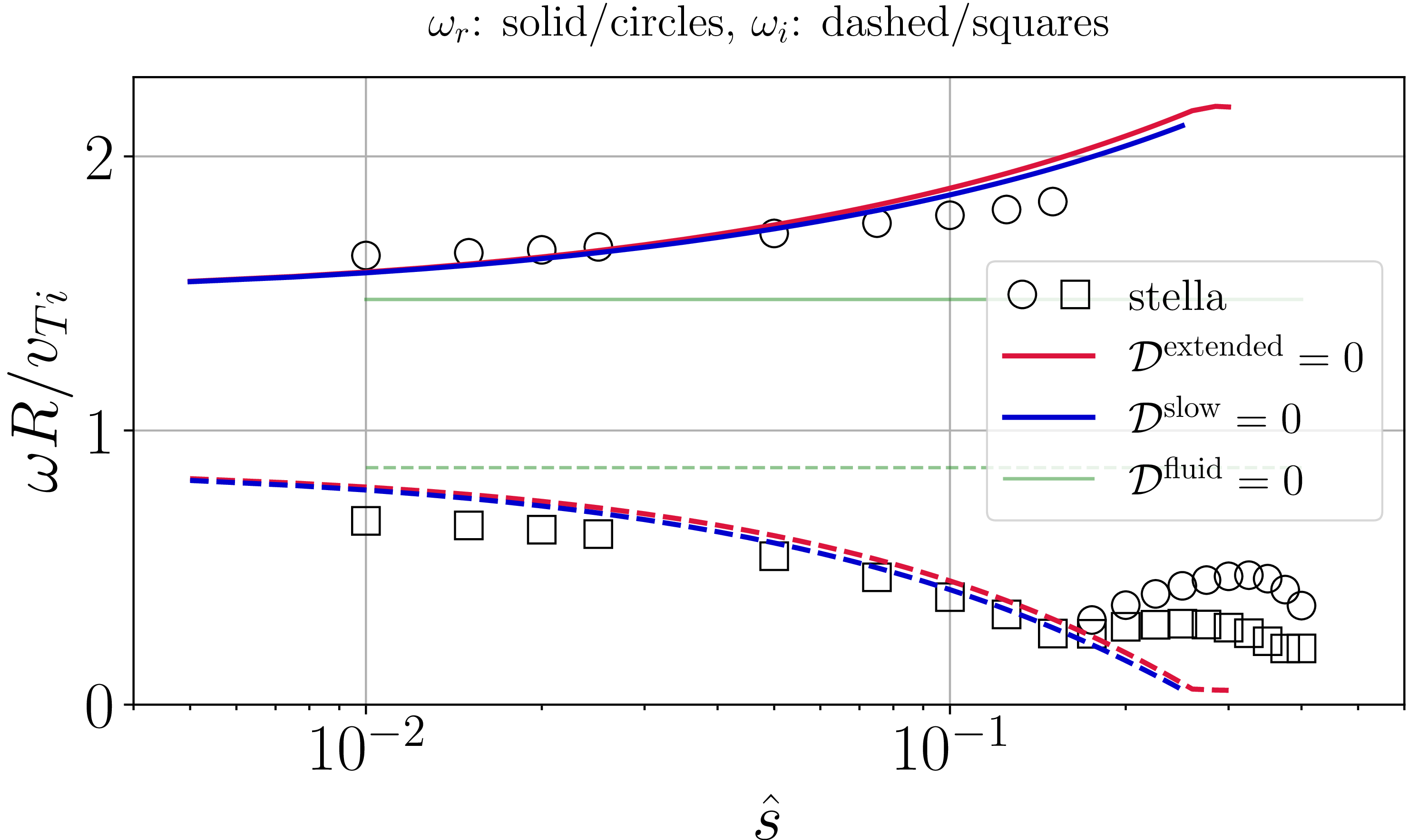


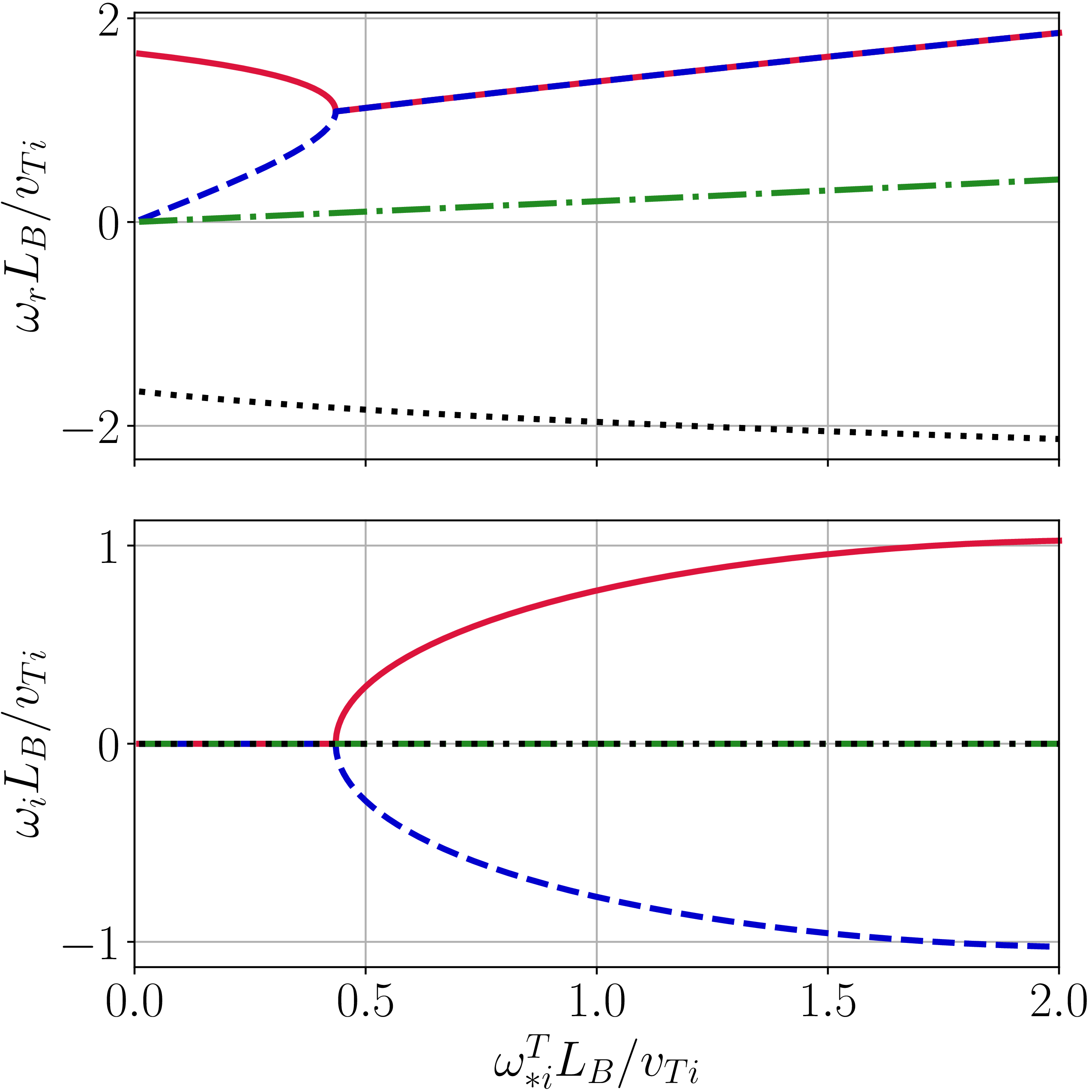
 ω∗i=0
 b¯i0/ω¯Mi02=LB2/vTi2
 τ=1
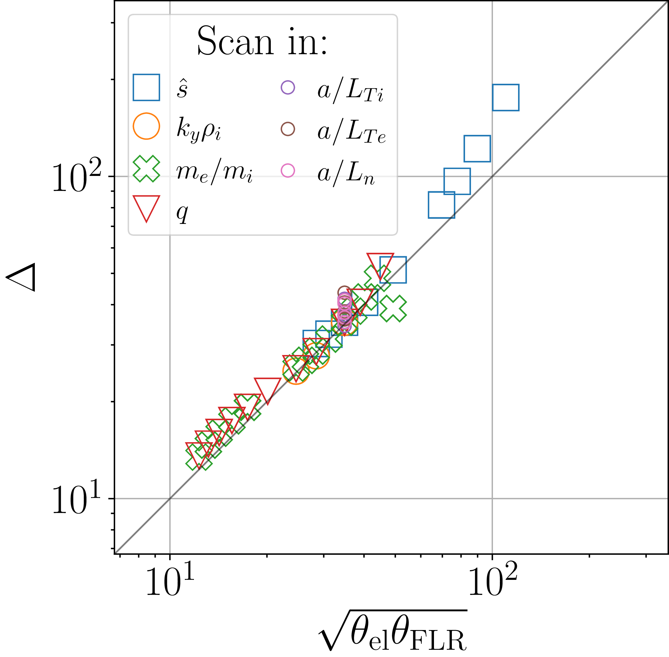
 Δ
 θel=q−1(me/mi)−1/2
 θFLR=(kyρis^)−1
 10%
 |1−ωsim/ωtheory|<0.1
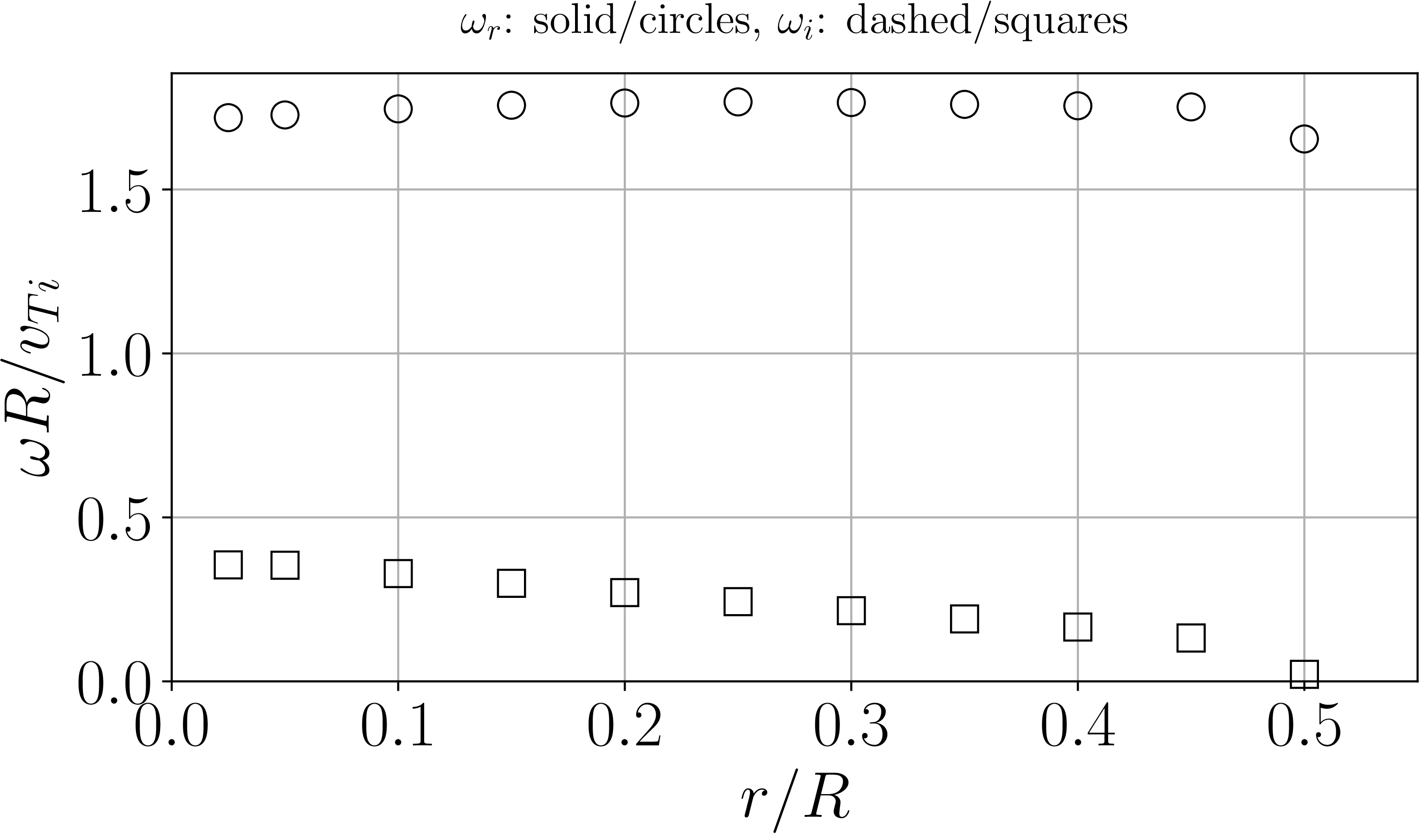
 r/R
 r/R≳0.5

 kyρi≲0.2

 eδφ/Ti(a/ρi)
 θ=0

 Open access

