1 Introduction
In this paper, we establish the existence and uniqueness of equilibrium states for Viana maps under a natural small-oscillation condition on the potential. The equilibrium state we derive is a Gibbs measure that satisfies a global upper Gibbs property. This enables us to obtain an upper level-2 large deviation principle.
Viana maps form an influential class of non-uniformly expanding surface endomorphisms obtained as skew-products of an expanding circle map with a perturbed quadratic family on the fibers [Reference VianaVia97]. Along the one-dimensional central bundle, the derivative is, in principle, expanding; however, whenever an orbit slips into the critical line
 $t=0$
, the quadratic term folds the fiber, sharply reducing the local derivative and diluting the accumulated expansion. This intermittent weakening prevents the system from being Anosov while still permitting a rich thermodynamic theory.
Let
 $f :M \rightarrow M$
be a continuous map on a compact smooth manifold. Among the invariant probability measures for the system, thermodynamic formalism identifies distinguished measures called equilibrium states; these are measures that maximize the quantity
 $h_{\mu }(f)+ \int \varphi \,d\mu $
, where
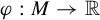 $\varphi :M \rightarrow {\mathbb {R}}$
is a potential function.
Classically, Bowen showed that for a mixing uniformly hyperbolic system, the combination of expansivity and the specification property ensures both existence and uniqueness of equilibrium states for every Hölder potential [Reference BowenBow74]. Climenhaga and Thompson later extracted the main ingredient of Bowen’s argument and recast it in a flexible orbit-decomposition framework that works beyond uniform hyperbolicity [Reference Climenhaga and ThompsonCT16]. Their technique measures the topological pressure carried by ‘obstructions’ to expansivity and specification; if these obstructions have strictly smaller pressure than the whole system, a unique equilibrium state still exists. In recent years, the Climenhaga–Thompson machinery has been applied extensively to construct equilibrium states in a range of settings:
-
(1) Mañé diffeomorphisms [Reference Climenhaga, Fisher and ThompsonCFT19] and the Katok map [Reference WangWan21];
-
(2) geodesic flows on manifolds of non-positive curvature [Reference Burns, Climenhaga, Fisher and ThompsonBCFT18, Reference Call and ThompsonCT22] and on surfaces without conjugate points [Reference Climenhaga, Knieper and WarCKW21];
-
(3) Lorenz flows with singularities [Reference Pacifico, Yang and YangPYY22];
-
(4) geodesic flows on flat surfaces with singularities [Reference Call, Constantine, Erchenko, Sawyer and WorkCCE + 22].
Using this generalization, we show that for Viana maps, every Hölder continuous function whose oscillation is below an explicit threshold admits a unique equilibrium state. The proof adapts the Climenhaga–Thompson machinery: we carve the dynamics into a ‘good’ core that enjoys specification and the Bowen property, and a ‘bad’ tail whose pressure we show is strictly lower than the topological pressure.
One benefit of [Reference BowenBow74, Reference Climenhaga and ThompsonCT16] is the construction of the unique equilibrium state as a Gibbs measure. In [Reference BowenBow74], the lower Gibbs property is essential in ruling out mutually singular equilibrium states. This approach is generalized in [Reference Climenhaga and ThompsonCT16], in which Climenhaga and Thompson derive the lower Gibbs property of equilibrium state for the ‘essential collection of orbit segments’ which dominates in pressure as well as a global upper Gibbs property for all orbit segments.
Based on this property, we are able to deduce an upper bound for the level-2 large deviation principle for the equilibrium state of Viana maps. In general, the large deviation principle describes the exponential rate of convergence of time average to the space average with respect to a given measure.
Before stating the main theorem, recall Viana’s construction. We refer to §3 for a more detailed discussion of the dynamical properties of Viana maps.
Definition 1.1. (Viana map)
Consider the map
 $$ \begin{align*} f_{\alpha}(\theta,t)= (d\theta\, \mod 1,\, a_0-t^2+\alpha \sin (2\pi\theta)), \quad (\theta,t)\in S^{1}\times {\mathbb{R}}. \end{align*} $$
Here,
 $d \geq 2$
is an integer,
 $\alpha $
is a small real number and the parameter
 $a_0 \in (1, 2)$
is such that the map
 $h(t) = a_0 - t^2$
has a pre-periodic (but not periodic) critical point. For
 $\alpha $
small enough, there is an interval
 $I \subset (-2,2)$
for which
 $f_{\alpha }(S^1\times I) \subset \mathrm {int}(S^1\times I)$
.
In [Reference VianaVia97], Viana constructed this quadratic skew-product over the linear strongly expanding map of the circle and proved that if
 $d\geq 16$
, then there exists a positive constant
 $c_0> 0$
such that any map f sufficiently
 $C^{3}$
-close to
 $f_{\alpha }$
has both Lyapunov exponents greater than
 $c_0$
Lebesgue-almost everywhere. Buzzi, Sester, and Tsujii later in [Reference Buzzi, Sester and TsujiiBST03] proved that if
 $d\ge 2$
, then for every sufficiently small
 $\alpha>0$
, the same is true in a
 $C^{\infty }$
-neighborhood.
1.1 Statement of main results
The principal result of this paper is the following.
Theorem A. For all
 $d\ge 16$
and
 $\epsilon>0$
sufficiently small, there is an
 $\alpha _0>0$
such that for all
 $\alpha \le \alpha _0$
and all Hölder potentials with
 $\sup \varphi -\inf \varphi <({c_0}/{2})-\log ({d+\epsilon }/{d-\epsilon })$
, the Viana map
 $f_{\alpha }$
has a unique equilibrium state
 $\mu $
for
 $\varphi $
. Moreover,
 $\mu $
has the upper level-2 large deviations principle.
Our proof is designed so that every step survives small perturbations to the dynamics. In particular, the expansivity, specification, and Bowen property we establish for
 $f_{\alpha }$
remain valid for all maps in a sufficiently small
 $C^{3}$
neighborhood. This robustness yields the following extension.
Theorem B. The same result in Theorem A is true for any sufficiently small
 $C^{3}$
perturbation of
 $f_{\alpha }$
(which is not necessarily a skew-product).
Henceforth, we use the term Viana map for any map f that lies in a sufficiently small
 $C^{3}$
-neighborhood of the reference skew product
 $f_{\alpha }$
. Unless explicitly stated otherwise, every result we state for a Viana map therefore applies simultaneously to
 $f_{\alpha }$
itself and to all its
 $C^{3}$
perturbations within this neighborhood.
In this paper, we study Viana maps on the forward-invariant region
 $S^1 \times I$
from Definition 1.1. For such a map f, we set
 $$ \begin{align*} \Lambda := \bigcap_{n \ge 0} f^n(S^1 \times I), \end{align*} $$
which equals
 $f^2(S^1 \times I)$
once I is chosen as in Viana’s construction. All notions of pressure and equilibrium states in Theorems A and B are taken for the restriction
 ${f|_\Lambda : \Lambda \to \Lambda }$
, that is, among f-invariant Borel probability measures supported on
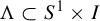 $\Lambda \subset S^1 \times I$
.
We briefly situate our results within the existing literature on Viana maps. Alves proved existence and uniqueness of the SRB measure [Reference AlvesAlv00]. Arbieto, Matheus, and Senti later established existence of equilibrium states for Hölder potentials with sufficiently small oscillation in an unpublished preprint [Reference Arbieto, Matheus and SentiAMS05]. Pinheiro and Varandas extended uniqueness to every Hölder potential whose oscillation is below a threshold [Reference Pinheiro and VarandasPV23]. Recently, using the countable Markov coding approach, Lima, Obata, and Poletti also obtained uniqueness of the measure of maximal entropy [Reference Lima, Obata and PolettiLOP26]. Alves, Oliveira, and Santana employed an inducing scheme to establish existence and finiteness of the measure of maximal entropy [Reference José, Alves and SantanaAOS24]; and Bilbao and Santana studied equilibrium states for zooming systems, obtaining stability and uniqueness under topological exactness, a framework that includes Viana attractors [Reference Bilbao and SantanaBS25].
The present work complements these results in several ways: Theorems A and B give a coding-free and robust proof of existence and uniqueness for all Hölder potentials whose oscillation is below an explicit, computable threshold, in a form that is uniform over a whole
 $C^3$
-neighborhood of the reference Viana map and, hence, applies to non-skew perturbations; in addition, the Climenhaga–Thompson decomposition we build yields a weak Gibbs description of the equilibrium state and an upper level-2 large deviation principle. Moreover, to the best of our knowledge, this provides the first example of the Climenhaga–Thompson machinery being implemented in a non-invertible setting with critical points.
We conclude the introduction with a road-map of the paper.
-
• Section 2 reviews the decomposition–obstruction framework of Climenhaga–Thompson and the necessary concepts from thermodynamic formalism.
-
• Section 3 recalls Viana’s construction and compiles the dynamical properties used later.
-
• Section 4 discusses non-uniformly expanding maps and summarizes Alves’s notion of hyperbolic times.
-
• Section 5 proves that Viana maps are non-uniformly expansive by showing that the set of non-expansive points carries pressure strictly below the topological pressure.
-
• Section 6 establishes a non-uniform specification property by demonstrating that most orbit segments satisfy specification.
-
• Section 7 combines these ingredients to prove the main theorem and, as a consequence of the Gibbs property, derives a large-deviation principle.
2 Background and main technique
We state the preliminary definitions needed for the technique and introduce how to apply the technique to deduce the desired thermodynamic formalism.
2.1 Pressure
Let
 $f : X \to X$
be a continuous map on a compact metric space. We identify the set
 $X \times \mathbb {N}$
with the space of finite orbit segments by identifying
 $(x, n)$
with
 $(x, f(x), \ldots , f^{n-1}(x)).$
The Bowen metric of order n associated to f is defined by
 $$ \begin{align*} d_n(x,y) = \max_{0 \le k < n} d(f^k(x), f^k(y)). \end{align*} $$
Given
 $x \in X$
,
 $\epsilon> 0$
, and
 $n \in \mathbb {N}$
, the Bowen ball of order n with center x and radius
 $\epsilon $
is
 $$ \begin{align*} B_n(x, \epsilon) = \{y \in X : d_n(x, y) < \epsilon\}. \end{align*} $$
A set
 $E \subset X$
is called
 $(n, \epsilon )$
-separated if
 $$ \begin{align*} d_n(x, y)\, \ge\, \epsilon \quad\text{for all } x, y \in E \text{ with } x \neq y. \end{align*} $$
Given
 $\mathcal {D} \subset X \times \mathbb {N}$
, we interpret
 $\mathcal {D}$
as a collection of finite orbit segments. Define
 $$ \begin{align*} \mathcal{D}_n = \{ x \in X : (x, n) \in \mathcal{D} \}, \end{align*} $$
the set of initial points of all length-n orbit segments in
 $\mathcal {D}$
. We then consider the corresponding partition sum
 $$ \begin{align*} \Lambda_n^{\mathrm{sep}} (\mathcal{D}, \varphi, \epsilon; f) = \sup \bigg\{\!\sum_{x \in E} e^{S_n \varphi(x)} : E \subset \mathcal{D}_n \text{ is } (n,\epsilon)\text{-separated}\bigg\}. \end{align*} $$
Definition 2.1. (Pressure)
The pressure of
 $\varphi $
on
 $\mathcal {D}$
at scale
 $\epsilon $
is given by
 $$ \begin{align*} P(\mathcal{D}, \varphi, \epsilon; f) = \limsup_{n \to \infty} \dfrac{1}{n} \log \Lambda_n^{\mathrm{sep}}(\mathcal{D}, \varphi, \epsilon; f). \end{align*} $$
Then, the pressure of
 $\varphi $
on
 $\mathcal {D}$
is defined as
 $$ \begin{align*} P(\mathcal{D}, \varphi; f) = \lim_{\epsilon \to 0}\, P(\mathcal{D}, \varphi, \epsilon; f). \end{align*} $$
Given
 $Z \subset X$
, define
 $$ \begin{align*} P(Z, \varphi, \epsilon; f) := P(Z \times \mathbb{N}, \varphi, \epsilon; f). \end{align*} $$
Observe that
 $P(Z, \varphi; f)$
denotes the usual upper capacity pressure [Reference BowenBow74] and we often write
 $P(\varphi; f)$
in place of
 $P(X, \varphi; f)$
for the pressure on the entire space.
When
 $\varphi = 0$
, our definition yields the entropy of
 $\mathcal {D}$
:
 $$ \begin{align} h(\mathcal{D}, \epsilon; f) = h(\mathcal{D}, \epsilon) := P(\mathcal{D}, 0, \epsilon) \quad\text{and}\quad h(\mathcal{D}) = \lim_{\epsilon \to 0} h(\mathcal{D}, \epsilon). \end{align} $$
Definition 2.2. (Equilibrium state)
Let
 $\mathcal {M}(f)$
be the set of f-invariant Borel probability measures and
 $\mathcal {M}_e(f)$
the subset of ergodic measures in
 $\mathcal {M}(f)$
. By the variational principle for pressure [Reference WaltersWal82, Theorem 9.10],
 $$ \begin{align*} P(\varphi; f) = \sup_{\mu \in \mathcal{M}(f)}\bigg(h_\mu(f) + \int \varphi \,d\mu \bigg) = \sup_{\mu \in \mathcal{M}_e(f)}\bigg(h_\mu(f) + \int \varphi \,d\mu\bigg). \end{align*} $$
A measure achieving this supremum is called an equilibrium state.
2.2 Obstructions to expansivity, specification, and regularity
Bowen showed in [Reference BowenBow74] that if
 $(X, f)$
is expansive and has the specification property, and if
 $\varphi $
satisfies certain regularity conditions, then there is a unique equilibrium state. We recall definitions and results from [Reference Climenhaga and ThompsonCT16], which demonstrate that non-uniform analogs of Bowen’s hypotheses are sufficient to guarantee uniqueness.
2.2.1 Expansivity
Given a continuous map
 $f : X \to X$
, the infinite Bowen ball of size
 $\epsilon> 0$
around a point
 $x \in X$
is defined by
 $$ \begin{align*} \Gamma_\epsilon(x) := \{ y \in X : d(f^k x, f^k y) < \epsilon \text{ for all } k \in \mathbb{{\mathbb{N}}} \}. \end{align*} $$
If there exists
 $\epsilon> 0$
such that
 $\Gamma _\epsilon (x) = \{x\}$
for every
 $x \in X$
, then we say that
 $(X, f)$
is positively expansive. Throughout the rest of the paper, we drop ‘positively’ and simply write expansive, since all maps under consideration are non-invertible.
Definition 2.3. For
 $f : X \to X$
, the set of non-expansive points at scale
 $\epsilon $
is defined by
 $$ \begin{align*} \mathrm{NE}(\epsilon) = \{ x \in X : \Gamma_\epsilon(x) \neq \{x\} \}. \end{align*} $$
An f-invariant measure
 $\mu $
is called almost expansive at scale
 $\epsilon $
if
 $\mu (\mathrm {NE}(\epsilon )) = 0$
.
Given a potential
 $\varphi $
, the pressure of obstructions to expansivity at scale
 $\epsilon $
is
 $$ \begin{align*} P_{\mathrm{exp}}^{\perp}(\varphi,\epsilon) &= \sup_{\mu \in \mathcal{M}_e(f)} \bigg\{h_\mu(f) + \int \varphi \, d\mu: \mu(\mathrm{NE}(\epsilon))> 0\bigg\}. \end{align*} $$
This quantity is non-increasing in
 $\epsilon $
, so we define a scale-free version by
 $$ \begin{align*} P_{\mathrm{exp}}^{\perp}(\varphi) = \lim_{\epsilon \to 0} P_{\mathrm{exp}}^{\perp}(\varphi,\epsilon). \end{align*} $$
In particular, the scale-free version
 $ P_{\exp }^{\perp }(\varphi ) $
satisfies
 $$ \begin{align*} P_{\exp}^{\perp}(\varphi) \le P_{\exp}^{\perp}(\varphi,\epsilon) \end{align*} $$
for any fixed
 $\epsilon> 0$
.
Roughly speaking,
 $ P^\perp _{\exp }(f,\epsilon ) $
can be understood as follows. Recall that positive expansivity is equivalent to the condition
 $$ \begin{align*} \bigcap_{n \ge 0} B_n(x,\epsilon) = \{x\}, \end{align*} $$
which holds for every
 $ x \in X $
when
 $\epsilon $
is sufficiently small. We define
 $ P^\perp _{\exp }(f,\epsilon ) $
to be the supremum of the pressures of all ergodic measures that assign positive weight to the set of points where this condition fails.
2.2.2 Specification
Definition 2.4. (W-specification at scale
 $\epsilon $
)

A collection of orbit segments
 $$ \begin{align*} \mathcal D \subset X\times{\mathbb{N}} \quad (\text{with } (x,n)\text{ representing the segment } x,\,f(x),\ldots,f^{n-1}(x)) \end{align*} $$
has the (W)-specification property at scale
 $\epsilon>0$
if there exists
 $\tau =\tau (\epsilon )\in {\mathbb {N}}$
such that, for every finite set of segments
 $$ \begin{align*} \{(x_j,n_j)\}_{j=1}^{k}\subset\mathcal D, \end{align*} $$
one can find ‘gluing times’
 $\tau _1,\ldots ,\tau _{k-1}\in {\mathbb {N}}$
with
 $\tau _i\le \tau $
for every i and a point
 $y\in X$
satisfying
 $$ \begin{align*} d_{n_j}\!(f^{t_{j}}(y),x_j)<\epsilon \quad\text{for each }1\le j\le k, \end{align*} $$
where
 $$ \begin{align*} t_1:=0,\quad t_j:=\sum_{i=1}^{j-1}(n_i+\tau_i)\quad (2\le j\le k). \end{align*} $$
Here,
 $d_{n}(x,y)=\max _{0\le m<n}d(f^{m}x,f^{m}y)$
is the Bowen metric of length n.
We say that
 $\mathcal {D}$
has the (W)-specification property if the above condition holds for every
 $\epsilon> 0$
. We say that
 $(X, f)$
has the (W)-specification property if
 $X \times \mathbb {N}$
does.
As in [Reference Climenhaga and ThompsonCT16], we will sometimes say that
 $\mathcal {G}$
has (W)-specification, or simply specification. This version of the specification is weak in the sense that the ‘transition times’
 $\tau _i$
are only assumed to be bounded by, rather than equal to,
 $\tau $
.
Definition 2.5. A triple
 $(\mathcal {P}, \mathcal {G}, \mathcal {S}) \subset (X \times \mathbb {N})^3$
is called a decomposition for
 $(X, f)$
if for every
 $x \in X$
and
 $n \in \mathbb {N}$
, there exist
 $p, g, s \in \mathbb {N}$
with
 $p + g + s = n$
such that
 $$ \begin{align*} (x, p) \in \mathcal{P},\quad (f^p x, g) \in \mathcal{G},\quad (f^{p+g} x, s) \in \mathcal{S}. \end{align*} $$
In other words, every orbit segment can be decomposed into a ‘prefix’ from
 $\mathcal {P}$
, a ‘good’ core from
 $\mathcal {G}$
, and a ‘suffix’ from
 $\mathcal {S}$
.
Note that the symbol
 $(x, 0)$
denotes the empty set and the functions
 $p, g, s$
are permitted to take the value zero.
Definition 2.6. The pressure of obstructions to specification at scale
 $\epsilon $
is defined by
 $$ \begin{align*} P_{\mathrm{spec}}^{\perp}(\varphi, \epsilon) := \inf \{P(\mathcal{P} \cup \mathcal{S},\varphi, 3\epsilon)\}, \end{align*} $$
where the infimum is taken over
 $\mathcal {P}, \mathcal {S} \subset X \times {\mathbb {N}}$
such that there exists a decomposition
 $(\mathcal {P},\mathcal {G},\mathcal {S}$
) for
 $(X,f)$
for which every
 $\mathcal {G}$
has specification at scale
 $\epsilon $
. We then define the scale-free version:
 $$ \begin{align*} P_{\mathrm{spec}}^{\perp}(\varphi) = \lim_{\epsilon \to 0} P_{\mathrm{spec}}^{\perp}(\varphi, \epsilon). \end{align*} $$
Again, since
 $P_{\mathrm {spec}}^{\perp }(\varphi , \epsilon )$
is monotonic as a function of
 $\epsilon $
, this limit exists. In contrast to
 $P_{\mathrm {exp}}^{\perp }(\varphi , \epsilon )$
,
 $P_{\mathrm {spec}}^{\perp }(\varphi , \epsilon )$
is non-decreasing in
 $\epsilon $
.
2.2.3 Regularity for potential
Definition 2.7. (Bowen property)
Given
 $\mathcal {D} \subset X \times \mathbb {N}$
, we say a function
 $\varphi : X \to \mathbb {R}$
has the Bowen property on
 $\mathcal {D}$
at scale
 $\epsilon $
if there is a constant
 $K = K(\varphi , \mathcal {D}, \epsilon )$
such that
 $$ \begin{align*} | S_n \varphi(x) - S_n \varphi(y) | < K \end{align*} $$
for every
 $(x, n) \in \mathcal {D}$
and every
 $y \in B_n(x, \epsilon )$
. A function
 $\varphi $
has the Bowen property on
 $\mathcal {D}$
if it satisfies the Bowen property on
 $\mathcal {D}$
at some scale
 $\epsilon $
(and thus at all smaller scales as well).
2.3 General results on uniqueness of equilibrium states
Our main tool for existence and uniqueness of equilibrium state is [Reference Climenhaga and ThompsonCT16, Theorem 5.5].
Theorem 2.8. [Reference Climenhaga and ThompsonCT16, Theorems 5.5 and 5.7]
Let X be a compact metric space and
 $f \colon X \to X$
a continuous map. Let
 $\varphi \colon X \to \mathbb {R}$
be a continuous potential function. Suppose that
 $$ \begin{align*} P_{\mathrm{exp}}^{\perp}(\varphi) < P_{\mathrm{top}}(\varphi) \end{align*} $$
and that
 $(X, f)$
admits a decomposition
 $(\mathcal {P}, \mathcal {G}, \mathcal {S})$
with the following properties:
-
(1)
$\mathcal {G}$
has (W)-specification at any scale; -
(2)
$\varphi $
has the Bowen property on
$\mathcal {G}$
; -
(3)
$P(\mathcal {P} \cup \mathcal {S}, \varphi ) < P(\varphi; f )$
.



Then, there is a unique equilibrium state
 $\mu $
for
 $\varphi $
. Moreover,
 $\mu $
satisfies the following upper large deviations bound: if A is any weak*-closed and convex subset of the space of Borel probability measures on X, then
 $$ \begin{align*} \limsup_{n\rightarrow\infty} \dfrac{1}{n} \log\mu(\mathcal{E}_n^{-1}(A)) \le \sup_{\nu\in A\cap \mathcal{M}(f)}\bigg(h_{\nu}(f)+ \int \varphi \,d\nu - P(\varphi; f)\bigg), \end{align*} $$
where
 $\mathcal {E}_n(x) = ({1}/{n})\sum _{k=0}^{n-1} \delta _{f^kx}$
is the nth empirical measure associated to x.
We note that the theorem we apply assumes that the pressures of obstructions to both expansivity and specification are defined in a scale-free manner.
3 Viana maps and their properties
We begin by gathering the necessary materials for the construction of Viana maps with the desired decomposition properties.
We consider from here on these maps f close to
 $f_{\alpha }$
restricted to
 $S^1 \times I$
. The main properties of f in a
 $C^3$
neighborhood of
 $f_{\alpha }$
are summarized below; see [Reference AlvesAlv00, Reference VianaVia97].
-
• Non-uniformly expanding, that is, for
$\alpha $
sufficiently small, there exists a positive constant
$c_0> 0$
such that any map f sufficiently close to
$f_{\alpha }$
in the
$C^3$
topology has both Lyapunov exponents greater than
$c_0$
at Lebesgue-almost every (a.e.) point, that is, for Lebesgue-a.e.
$x=(\theta , t) \in S^1 \times I$
,
$$ \begin{align*}\liminf_{n\rightarrow \infty} \dfrac{1}{n} \log \|Df^n(x)\|> c_0.\end{align*} $$
-
• Slow approximation to the critical set, that is, letting
denote the critical set of f, for every
$$ \begin{align*} \mathcal C := \{x \in S^1 \times I : \det|Df_x|=0\} \end{align*} $$
$\gamma>0$
, there exists
$\delta> 0$
such that for Lebesgue-a.e.
$x \in S^1 \times I$
,
$$ \begin{align*} \limsup_{n\rightarrow\infty} \dfrac{1}{n}\sum_{j=0}^{n-1} -\log [\mathrm{dist}_{\delta}(f^j(x),\mathcal{C})]\leq \gamma. \end{align*} $$
Here,
$\mathrm {dist}_{\delta }$
is the
$\delta $
-truncated distance defined by
$$ \begin{align*}\mathrm{dist}_{\delta}(x,\mathcal{C}) = \begin{cases} 1 &\quad \text{if }\mathrm{dist}(x,\mathcal{C}) \geq \delta,\\ \mathrm{dist}(x,\mathcal{C}) &\quad \text{otherwise}. \end{cases}\end{align*} $$
-
• Existence and uniqueness of an ergodic absolutely continuous invariant (SRB) measure
$\mu _{\mathrm {SRB}}$
. -
• The attractor of f within the forward-invariant region
$S^1 \times I$
is defined as the intersection of all forward images of
$$ \begin{align*} \Lambda =\bigcap_{n\geq 0} f^n(S^1\times I) \end{align*} $$
$S^1 \times I$
, which is just
$\Lambda = f^2(S^1 \times I)$
, as long as the interval I is properly chosen.
-
• Strongly topologically mixing: for any open set
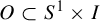
$ O \subset S^1 \times I $
, there exists
$n= n(O) \in \mathbb {N} $
such that
$$ \begin{align*} f^{n}(O) = \Lambda. \end{align*} $$








Next, we study the dynamics of the tangent bundle for Viana maps. Denote by
 $ f_0 $
the direct product map
 $$ \begin{align*} f_0 = g \times h: S^1 \times I \to S^1 \times I, \quad (\theta, t) \mapsto (d\theta\, \mod 1, a_0 - t^2). \end{align*} $$
Since
 $ Df_0 \cdot ({\partial }/{\partial \theta }) = d \cdot ({\partial }/{\partial \theta }) $
and
 $ Df_0 \cdot ({\partial }/{\partial t}) = -2t \cdot ({\partial }/{\partial t}) $
, with
 $ d \geq 16> 4 $
and
 $ I \subset (-2, 2) $
, it is clear that
 $ f_0 $
is a partially hyperbolic map of the form
 $ T_{(\theta ,t)}(S^1 \times I) = E^u \oplus E^c $
, where
 $ E^u $
is uniformly expanding and
 $ E^c $
is dominated by
 $ E^u $
. From the theory of partial hyperbolicity, we know that if
 $ \alpha $
is sufficiently small, the map
 $ f_{\alpha } $
(like any
 $ C^1 $
-nearby map) also admits a partially hyperbolic splitting of the form
 $ E^u \oplus E^c $
, which varies continuously. As a consequence, we get the following proposition.
Proposition 3.1. Given
 $\epsilon> 0$
, if
 $\alpha $
is sufficiently small, the Lyapunov exponent
 $$ \begin{align*}\unicode{x3bb}^u(x, f):= \lim_{n\rightarrow\infty}\frac{1}{n}\log \|Df^n|_{E^u(x)}\|\end{align*} $$
associated to
 $E^u$
at every point x satisfies
 $$ \begin{align*}\log(d-\epsilon)\leq \unicode{x3bb}^u(x, f) \leq \log(d+\epsilon)\end{align*} $$
for any f close to
 $f_{\alpha }$
.
By applying the previous theorems, we derive a lower bound on the entropy of the SRB measure
 $ \mu _{\mathrm {SRB}}$
. By Pesin’s formula, the entropy
 $ h_{\mu _{\mathrm {SRB}}}(f) $
of
 $ \mu _{\mathrm {SRB}} $
is given by the integrated sum of the positive Lyapunov exponents of
 $ \mu _{\mathrm {SRB}} $
. Therefore, by Proposition 3.1, we obtain the following bound:
 $$ \begin{align*} h_{\mu_{\mathrm{SRB}}}(f) \geq \log(d - \epsilon) + c_0. \end{align*} $$
4 Hyperbolic times and non-uniformly expanding maps
To advance the proof, we recall the notion of hyperbolic time for maps with a critical set, following the framework of Alves, Bonatti, and Viana [Reference Alves, Bonatti and VianaABV00], specialized to our partially hyperbolic setting.
Let
 $f\colon M \to M$
be a
 $C^2$
map that is a local diffeomorphism except on a set
 $\mathcal {C} \subset M$
of zero Lebesgue measure. We assume that there is a continuous
 $Df$
-invariant splitting
 $E^u \oplus E^c$
on M and a continuous cone field
 $\mathrm {Cone}^c = \{\mathrm {Cone}^c(x)\}_{x\in M}$
around
 $E^c$
such that
 $\mathrm {Cone}^c(x)$
contains the critical (center) direction at points of
 $\mathcal {C}$
.
We say that f is non-flat along the critical direction if there exist constants
 ${B>1}$
and
 $\ell>0$
such that, for all
 $x,y \notin \mathcal {C}$
with
 $2\,\mathrm {dist}(x,y) < \mathrm {dist}(x,\mathcal {C})$
and for every
 $v \in \mathrm {Cone}^c(x)\setminus \{0\}$
, we have:
-
•
$({1}/{B}) \mathrm {dist}(x, \mathcal {C})^l \leq {\|Df(x)v\|}/{\|v\|} \leq B \mathrm {dist}(x, \mathcal {C})^l;$
-
•
$|\!\log \!\|Df (x)^{-1}\|\!- \log \|Df (y)^{-1}\||\!\leq B ({\mathrm {dist}(x,y)}/{\mathrm {dist}(x, \mathcal {C})^l}) ;$
-
•
$|\!\log \!|\det Df (x)^{-1}|\!- \log \!|\det Df (y)^{-1}||\!\leq B ({\mathrm {dist}(x,y)}/{\mathrm {dist}(x, \mathcal {C})^l}).$



By dominated splitting and uniform control of the angle between
 $E^u$
and
 $E^c$
, these estimates along
 $\mathrm {Cone}^c$
are equivalent up to a uniform multiplicative constant to the corresponding estimates for the full operator norm
 $\|Df(x)^{-1}\|$
and the Jacobian
 $|\!\det Df(x)|$
, exactly as in [Reference Alves, Bonatti and VianaABV00].
In our application, we take
 $M = \Lambda $
,
 $\mathcal {C}$
equal to the critical set of the fiber map,
 $E^c$
the center bundle, and
 $\mathrm {Cone}^c$
a center cone field. As the reader can verify, the reference Viana map
 $f_{\alpha }$
satisfies these non-flatness assumptions along the center direction and since these conditions are
 $C^2$
-open, they hold for all Viana maps in a sufficiently small
 $C^2$
-neighborhood of
 $f_{\alpha }$
.
For the definition of hyperbolic times, we fix
 $0 < b < \min \{1/2, 1/(2\beta )\}$
.
Definition 4.1. Given
 $0 < \sigma < 1$
and
 $\delta> 0$
, we say that n is a
 $(\sigma ,\delta )$
-hyperbolic time for x if, for all
 $1 \leq k \leq n$
,
 $$ \begin{align*}\prod_{j=n-k}^{n-1}\|Df(f^j(x))^{-1}\| \leq \sigma^k\end{align*} $$
and
 $$ \begin{align*}\mathrm{dist}_{\delta}(f^{n-k}(x),\mathcal{C}) \geq \sigma^{bk}.\end{align*} $$
Hyperbolic times are useful because they have the following key property.
Lemma 4.2. [Reference Alves, Bonatti and VianaABV00, p. 377]
Given
 $\sigma < 1$
and
 $\delta> 0$
, there exists
 $\delta _1> 0$
such that if n is a
 $(\sigma ,\delta )$
-hyperbolic time of x, then there exists a neighborhood
 $V_x$
of x such that:
-
•
$f^n$
maps
$V_x$
diffeomorphically onto the ball
$B_{\delta _1}(f^n(x))$
; -
• for every
$1\leq k \leq n$
and
$y,z\in V_x$
,
$$ \begin{align*}\mathrm{dist}(f^{n-k}(y), f^{n-k}(z)) \leq \sigma^{k/2} \mathrm{dist}(f^n(y), f^n(z)).\end{align*} $$


Remark. In our setting, the non-flatness assumption is verified along the center direction, that is, on a
 $Df$
-invariant cone field
 $\mathrm {Cone}^c$
around
 $E^c$
and [Reference Alves, Bonatti and VianaABV00, Lemma 5.2] is applied to
 $\sup _{v\in \mathrm {Cone}^c(x), \|v\|=1}\|Df(x)^{-1}v\|$
. By dominated splitting and the uniform bound on the angle between
 $E^u$
and
 $E^c$
, there exists
 $C\ge 1$
such that
 $$ \begin{align*} \sup_{v\in \mathrm{Cone}^c(x), \|v\|=1}\|Df(x)^{-1}v\| \kern1.5pt{\le}\kern1.5pt \|Df(x)^{-1}\| \kern1.5pt{\le}\kern1.5pt C\,\kern-0.9pt\sup_{v\in \mathrm{Cone}^c(x), \|v\|=1}\kern-1pt\|Df(x)^{-1}v\| \kern-1pt\quad\text{for all }x, \end{align*} $$
so the notion of
 $(\sigma ,\delta )$
-hyperbolic time used in Definition 4.1, which is formulated with the full operator norm
 $\|Df^{-1}\|$
, is equivalent to the one used in [Reference Alves, Bonatti and VianaABV00], up to adjusting
 $\sigma $
. Thus, Lemma 4.2 is precisely [Reference Alves, Bonatti and VianaABV00, Lemma 5.2] adapted to our center cone field setting.
Definition 4.3. For a fixed
 $\sigma <1$
, we define the expanding set
 $H(\sigma )$
to be the set of points
 $x\in M$
with the following two properties:
 $$ \begin{align*}\limsup_{n\rightarrow \infty} \dfrac{1}{n}\sum_{j=0}^{n-1}\log\|Df(f^j(x)^{-1})\| \leq 3\log\sigma < 0\end{align*} $$
and, for any
 $\gamma> 0$
, there is some
 $\delta> 0$
satisfying
 $$ \begin{align*}\limsup_{n\rightarrow \infty} \dfrac{1}{n}\sum_{j=0}^{n-1}-\log(\mathrm{dist}_{\delta}(f^j(x),\mathcal{C})) \leq \gamma.\end{align*} $$
Proposition 4.4. [Reference Alves, Bonatti and VianaABV00, p. 379]
Given
 $\sigma < 1$
, there exist
 $\nu> 0$
and
 $\delta> 0$
depending only on
 $\sigma $
and f such that, given any
 $x \in H(\sigma )$
and
 $N \geq 1$
sufficiently large, there are
 $(\sigma ,\delta )$
-hyperbolic times
 $1\leq n_1 <\cdots <n_l \leq N$
for x with
 $l\geq \nu N$
.
5 Non-uniform expansivity
In this section, we show that Viana maps are systems for which expansivity fails, but this failure occurs in a lower entropy setting, giving rise to a form of non-uniform expansivity.
5.1 Non-expansive set
We first explain how Viana maps fail to be expansive. A key source of non-expansivity in Viana maps is the repeated folding of points on the fiber direction. More precisely, one constructs a small vertical segment crossing the critical set
 $\{t=0\}$
and observes that its forward image is folded by the quadratic term
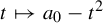 $t\mapsto a_0-t^2$
. Although iterates away from the critical region could, in principle, separate points, the skew-product structure makes it possible that for some choice
 $\theta $
, this same vertical segment (or a small sub-segment of it) is returned to the critical region sufficiently often, so that before substantial divergence occurs, another iterate causes it to fold again. This process produces pairs of distinct points whose forward orbits remain arbitrarily close for all times. In particular, for any arbitrarily small
 $\epsilon $
, there always exist distinct points whose orbits remain
 $\epsilon $
-close for every iterate, so the infinite Bowen ball of size
 $\epsilon $
never degenerates to a single point. Consequently, Viana maps fail to be expansive at every scale.
5.2 Slow recurrence
To overcome the loss of expansion caused by folding, we need to control the recurrence to the critical set
 $\mathcal {C}$
of generic points of invariant ergodic measures whose Lyapunov exponents are regular.
Lemma 5.1. Let
 $\eta $
be an ergodic measure such that
 $\unicode{x3bb} ^c(\eta )> -\infty $
, where
 $\unicode{x3bb} ^c$
is the Lyapunov exponent of
 $\eta $
associated to
 $E^c$
. Then,
 $$ \begin{align*}\int |\!\log \mathrm{dist} (x, \mathcal{C})| \,d\eta < \infty.\end{align*} $$
Proof. Since
 $\eta $
is ergodic,
 $\unicode{x3bb} ^c(\eta ) = \int \log \|Df|_{E^c}\|\,d\eta> -\infty $
. However, the definition of
 $f_{\alpha }$
and
 $\alpha $
sufficiently small implies
 $\tfrac 13 \|Df(x)|_{E^c}\| \leq \mathrm {dist} (x, \mathcal {C}) \leq 3 \|Df(x)|_{E^c}\|$
. These two facts together finish the proof.
Lemma 5.2. Let
 $\eta $
be an ergodic measure with
 $\unicode{x3bb} ^c(\eta )> -\infty $
. Then, for any
 $\gamma> 0$
, there exists
 $\delta> 0$
such that for
 $\eta $
-a.e. point x,
 $$ \begin{align*} \limsup_{n \to \infty} \dfrac{1}{n} \sum_{j=0}^{n-1}(-\!\log \mathrm{dist}_\delta(f^j(x), \mathcal{C})) \le \gamma. \end{align*} $$
Proof. By Lemma 5.1, the function
 $|\!\log \mathrm {dist}(x, \mathcal {C})|$
is
 $\eta $
-integrable and, in particular,
 $\eta (\mathcal {C}) = 0$
. Using these facts together with the definition of the
 $\delta $
-truncated distance
 $\mathrm {dist}_\delta $
, we deduce that for any
 $\gamma> 0$
, there exists
 $\delta> 0$
such that
 $$ \begin{align*} \int -\log \mathrm{dist}_\delta(x,\mathcal{C}) \, d\eta \le \gamma. \end{align*} $$
Because
 $\eta $
is ergodic, an application of Birkhoff’s ergodic theorem to the function
 $-\log \mathrm {dist}_\delta (x, \mathcal {C})$
completes the proof.
5.3 Almost expansivity
Next, we prove that, for Viana maps, any ergodic f-invariant measure with large pressure must be positively expansive. We prove this using the strategy outlined below; see [Reference Arbieto, Matheus and SentiAMS05, Reference OliveiraOli03].
-
• Select a certain set
$\mathcal {K}$
of ergodic f-invariant measures, which are natural candidates for attaining the variational principle. -
• Prove that any measure outside
$\mathcal {K}$
have strictly smaller pressure than the topological pressure hence cannot be an equilibrium state. -
• Show that any measure inside
$\mathcal {K}$
is an expanding measure and any expanding measure is almost positively expansive.


We begin by describing
 $\mathcal {K}$
, the set of candidate measures for achieving the variational principle. Define
 $$ \begin{align*} \mathcal{K} = \bigg\{\mu \in \mathcal{M}_e(f):\unicode{x3bb}^c(\mu)> \dfrac{c_0}{3}\bigg\}. \end{align*} $$
That is,
 $\mathcal {K}$
consists of those ergodic f-invariant measures whose central Lyapunov exponent is strictly bounded below by
 ${c_0}/{3}$
. The set
 $\mathcal {K}$
is non-empty, as it contains the unique SRB measure
 $\mu _{\mathrm {SRB}}$
, which has
 $\unicode{x3bb} ^c(\mu _{\mathrm {SRB}})> c_0$
by Pesin’s entropy formula.
5.3.1 Low pressure outside
$\mathcal {K}$

The measures in
 $\mathcal {K}$
are natural candidates for realizing the variational principle because the measures outside of
 $\mathcal {K}$
have small pressure.
Lemma 5.3. For every
 $\eta \notin \mathcal K$
,
 $$ \begin{align*} h_{\eta}(f)+\int \varphi\,d\eta \le P(\varphi;f)-\frac{c_0}{6}. \end{align*} $$
In particular,
 $$ \begin{align*} \sup_{\eta\in\mathcal M_e(f)\setminus\mathcal K} \bigg\{h_{\eta}(f)+\int \varphi\,d\eta\bigg\} \le P(\varphi;f)-\frac{c_0}{6}. \end{align*} $$
Proof. We compare
 $h_{\eta }(f) + \int \varphi \, d\eta $
with
 $h_{\mu _{\mathrm {SRB}}}(f) + \int \varphi \, d\mu _{\mathrm {SRB}}$
. Since
 $\eta \notin \mathcal {K}$
, it follows that
 $\unicode{x3bb} ^c(\eta ) \le ({c_0}/{3})$
. Therefore,
 $$ \begin{align*} h_{\eta}(f) + \int \varphi \, d\eta &\le \log(d+\epsilon) +\frac{c_0}{3}+ \int \varphi \, d\eta \\ &\le \log(d+\epsilon) +\frac{c_0}{3} + \int \varphi \, d\mu_{\mathrm{SRB}} + (\sup\varphi-\inf\varphi) \\ &< \log(d+\epsilon) +\frac{c_0}{3} + \bigg(\frac{c_0}{2}-\log \frac{d+\epsilon}{d-\epsilon}\bigg)+ \int \varphi \, d\mu_{\mathrm{SRB}} \\ &= \log(d-\epsilon)+\frac{5c_0}{6}+\int \varphi \, d\mu_{\mathrm{SRB}} \\ &\le h_{\mu_{\mathrm{SRB}}}(f) + \int \varphi \, d\mu_{\mathrm{SRB}} -\frac{c_0}{6}. \end{align*} $$
Here, the first inequality follows from Ruelle’s inequality, with the unstable Lyapunov exponent at most
 $\log (d+\epsilon )$
. The second inequality uses
 $\int \varphi \,d\eta \le \int \varphi \,d\mu _{\mathrm {SRB}}+(\sup \varphi -\inf \varphi )$
. The strict inequality uses our assumption
 $\sup \varphi - \inf \varphi < ({c_0}/{2})-\log ({(d+\epsilon)}/{(d-\epsilon)})$
. The last inequality uses Pesin’s entropy formula so that
 $h_{\mu _{\mathrm {SRB}}}(f)\ge \log (d-\epsilon )+c_0$
. By the variational principle, this proves that
 $h_{\eta }(f) + \int \varphi \, d\eta \le P(\varphi; f )-({c_0}/{6})$
.
5.3.2 Expanding measures
We define the notion of expanding measures originally introduced in [Reference Alves, Bonatti and VianaABV00].
Definition 5.4. A measure
 $\mu $
is called a
 $\sigma ^{-1}$
-expanding measure if
 $x \in H(\sigma )$
for
 $\mu $
-a.e. point x. In other words,
 $\mu (H(\sigma )) = 1$
. Here,
 $H(\sigma )$
is the
 $\sigma ^{-1}$
-expanding set defined in Definition 4.3.
We now show that there exists a single
 $\sigma> 1$
such that every
 $\mu \in \mathcal {K}$
is
 $\sigma ^{-1}$
-expanding. As will become clear later, a uniform choice of
 $\sigma $
across all
 $\mu \in \mathcal {K}$
is necessary for establishing that every ergodic measure in
 $\mathcal {K}$
is almost expansive at the same scale.
Lemma 5.5. Any
 $\mu \in \mathcal {K}$
is
 $\sigma ^{-1}$
-expanding with
 $\sigma = \exp (-{c_0}/{9})$
.
Proof. Since
 $\mu $
is ergodic, we have
 $$ \begin{align*} \unicode{x3bb}^c(x) = \unicode{x3bb}^c(\mu) = \int \log\|Df(x)|_{E^c}\| \, d\mu> \frac{c_0}{3} \end{align*} $$
for
 $\mu $
-a.e. x. By Birkhoff’s ergodic theorem, this is equivalent to
 $$ \begin{align*} \lim_{n \to \infty} \dfrac{1}{n} \sum_{j=0}^{n-1} \log \|Df(f^j(x))^{-1}\| \leq 3 \cdot \bigg( -\frac{c_0}{9} \bigg) < 0, \end{align*} $$
because the central direction
 $E^c$
is one-dimensional.
This fact, combined with Lemma 5.2, gives us the assumptions needed for
 $H(\sigma )$
at
 $\mu $
-a.e. point.
5.3.3 Expansivity inside
$\mathcal {K}$

Finally, we conclude the proof that any
 $\sigma ^{-1}$
-expanding measure
 $\mu $
is almost expansive at scale
 $\delta _1$
, which implies every
 $\mu \in \mathcal {K}$
is almost expansive.
Lemma 5.6. For any
 $\sigma ^{-1}$
-expanding measure
 $\mu $
, there exists
 $\delta _1> 0$
such that for any
 $\epsilon < \delta _1$
and for
 $\mu $
-a.e. x,
 $$ \begin{align*} \Gamma_{\epsilon}(x) = \{x\}. \end{align*} $$
Proof. Proposition 4.4 guarantees that for
 $\mu $
-a.e. x, there are infinitely many hyperbolic times
 $n_i(x)$
, since
 $\mu $
is
 $\sigma ^{-1}$
-expanding. Therefore, applying Lemma 4.2, we conclude that there exists some
 $\delta _1> 0$
such that if
 $y \in \Gamma _{\epsilon }(x)$
with
 $\epsilon < \delta _1$
, then for any
 $n_i$
, we have
 $$ \begin{align*} \text{dist}(x, y) \leq \sigma^{n_i/2} \, \text{dist}(f^{n_i}(x), f^{n_i}(y)) \leq \sigma^{n_i/2} \epsilon. \end{align*} $$
Since
 $n_i \to \infty $
as
 $i \to \infty $
, we deduce that
 $x = y$
.
5.4 Pressure gap
Theorem 5.7. We have the pressure gap
 $$ \begin{align*} P_{\mathrm{exp}}^{\perp}(\varphi) < P(\varphi; f ). \end{align*} $$
Proof. By definition, for any
 $\epsilon < \delta _1$
,
 $$ \begin{align*} P_{\mathrm{exp}}^{\perp}(\varphi,\epsilon) = \sup_{\mu \in \mathcal{M}_e(f)} \bigg\{h_\mu(f) + \int \varphi \, d\mu : \mu(\mathrm{NE}(\epsilon))> 0\bigg\}. \end{align*} $$
Consider two cases for a measure
 $\mu $
.
Case 1:
 $\mu \notin \mathcal {K}$
. By Lemma 5.3, we have a uniform bound:
 $$ \begin{align*} h_{\mu}(f)+\int \varphi\,d\mu < P(\varphi; f )- \frac{c_0}{6}. \end{align*} $$
In particular,
 $$ \begin{align*} \sup_{\mu\in\mathcal M_e(f)\setminus\mathcal K} \bigg\{h_{\mu}(f)+\int \varphi\,d\mu\bigg\} \le P(\varphi;f)-\frac{c_0}{6}. \end{align*} $$
Hence, such measures cannot achieve a pressure at
 $P(\varphi; f )$
.
Case 2:
 $\mu \in \mathcal {K}$
. By Lemma 5.6, there exists
 $\delta _1> 0$
so that for all
 $\epsilon < \delta _1$
,
 $$ \begin{align*} \mu(\mathrm{NE}(\epsilon)) = 0. \end{align*} $$
Thus, for sufficiently small
 $\epsilon $
, these measures place no mass on
 $\mathrm {NE}(\epsilon )$
and do not contribute to
 $P_{\mathrm {exp}}^{\perp }(\varphi ,\epsilon )$
.
In summary, for small enough
 $\epsilon $
, every measure that contributes to
 $P_{\mathrm {exp}}^{\perp }(\varphi ,\epsilon )$
lies outside
 $\mathcal {K}$
, and each such measure has pressure below
 $P(\varphi; f )$
. Consequently,
 $$ \begin{align*} P_{\mathrm{exp}}^{\perp}(\varphi) = \lim_{\epsilon\rightarrow 0} P_{\mathrm{exp}}^{\perp}(\varphi,\epsilon) < P(\varphi; f ). \end{align*} $$
This completes the proof.
6 Non-uniform specification and regularity
In this section, we first give an explicit description of how to decompose the collection of all orbit segments
 $(x,n)$
into
 $(\mathcal {P}, \mathcal {G},\mathcal {S})$
. We show that
 $\mathcal {G}$
has the specification property at any scale
 $\varepsilon $
and that orbits not in
 $\mathcal {G}$
carry small pressure. In addition, any Hölder continuous
 $\varphi $
has the Bowen property on
 $\mathcal {G}$
at some fixed scale
 $\varepsilon _0$
.
6.1 Construction of the orbit decomposition
Let
 $\psi ^c(x) = \log \|Df|_{E^c(x)}\|$
, so that
 $({1}/{n}) S_n \psi ^c(x)$
represents the average expansion (or contraction) undergone by an orbit segment
 $(x, n)$
in the center direction. Additionally, given
 $\mu \in \mathcal {M}_e(f)$
,
 $\unicode{x3bb} ^c(\mu ) =\int \psi ^c\, d\mu $
is the center Lyapunov exponent of
 $\mu $
.
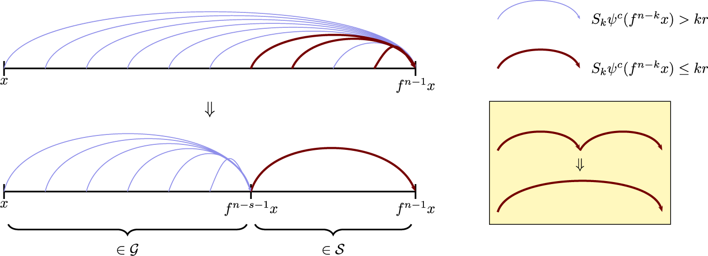
To define the orbit decomposition (Figure 1), for some small
 $r>0$
, we consider the following collection of orbit segments:
 $$ \begin{align} \begin{aligned} \mathcal{P} &:=\emptyset, \\ \mathcal{G} &:=\{(x,n)\in \Lambda\times {\mathbb{N}}:\,S_{k}\psi^c(f^{n-k}x)> kr \text{ for all }\, 0< k\leq n\},\\ \mathcal{S} &:=\{(x,n)\in \Lambda\times {\mathbb{N}}:\, S_n\psi^c(x) \le nr\}. \end{aligned} \end{align} $$
Orbit decomposition (color online).

Figure 1 Long description
The top panel shows a horizontal line from x at the left to f to the n minus 1 x at the right, with multiple arcs above. Blue arcs span from x to intermediate points, while red arcs cluster near the right endpoint. The lower panel, below a downward double arrow, shows the same interval split at f to the n minus s minus 1 x, with blue arcs on the left labeled as belonging to script G and red arcs on the right labeled as script S. The right side contains a legend: a blue arc is labeled S sub k psi superscript c open parenthesis f to the n minus k x close parenthesis greater than k r, a red arc is labeled S sub k psi superscript c open parenthesis f to the n minus k x close parenthesis less than or equal to k r. Below, a yellow box shows two red arcs above a single red arc, with a downward double arrow indicating merging. All labels and mathematical expressions are rendered exactly as shown.
The collection
 $\mathcal {G}$
is chosen so that along orbit segments from
 $\mathcal {G}$
, the center-unstable manifolds are uniformly backward contracting. In addition, f is locally invertible along these ‘good’ orbits.
Together with the trivial collection
 $\{(x,0) : x \in \Lambda \}$
for
 $\mathcal {P}$
, these collections define a decomposition of any orbit
 $(x, n) \in \Lambda \times \mathbb {N}$
as follows: let s be the largest integer in
 $\{0, \ldots , n\}$
such that
 $ S_{s}\psi ^c(f^{n-s}x) \le sr$
, meaning
 $(f^{n-s}x, s) \in \mathcal {S}$
.
We must then have
 $(x, n-s) \in \mathcal {G}$
, since if
 $S_{k_0}\psi ^c(f^{n-s-k_0} x) \le k_0r$
for some
 $0 < k_0 \leq n-s$
, then
 $$ \begin{align*} S_{s+k_0}\psi^c(f^{n-s-k_0}x) = S_{k_0}\psi^c(f^{n-s-k_0}x) + S_{s}\psi^c(f^{n-s}x) \le (s+k_0)r, \end{align*} $$
which would contradict the maximality of s.
6.2 Specification on
$\mathcal {G}$

In the uniformly hyperbolic setting, a key step in establishing specification on a mixing, locally maximal hyperbolic set
 $\Lambda $
is that for any
 $\delta> 0$
, there exists
 $N \in \mathbb {N}$
such that for all
 $x, y \in \Lambda $
and
 $n \ge N$
,
 $$ \begin{align*} f^n(W_\delta^u(x)) \cap W_\delta^s(y) \neq \varnothing. \end{align*} $$
For Viana maps, we adapt this idea by replacing the local stable manifold with the point y itself and the local unstable manifold with the center-unstable manifold
 $W_\delta ^{cu}(x)$
. Indeed, Viana maps can be viewed as partially hyperbolic systems with one-dimensional unstable and center directions. Because each center-unstable manifold is merely a two-dimensional disk and every such disk is eventually mapped onto
 $\Lambda $
by the strong mixing property, the same construction effectively applies.
To prove specification on
 $\mathcal {G}$
, we begin by establishing that every ‘good’ orbit in
 $\mathcal {G}$
exhibits backward uniform contraction.
Lemma 6.1. There exist
 $\varepsilon _0>0$
and
 $C\ge 1$
such that for every
 $(x,n)\in \mathcal G$
and every
 $y\in B_n(x,\varepsilon _0)$
, we have
 $$ \begin{align} d(f^k x, f^k y) < C e^{-r(n-1-k)}\, d(f^{n-1}x, f^{n-1}y) < C e^{-r(n-1-k)}\,\varepsilon_0 \end{align} $$
for all
 $0\le k\le n-1$
.
Proof. From
 $(x,n)\in \mathcal G$
and the definition of
 $\psi ^c$
, we obtain a uniform backward contraction along the center:
 $$ \begin{align*} \|Df^{-(n-1-k)}|_{E^c(f^{n-1} x)}\|< e^{-r(n-1-k)},\quad 0\le k\le n-1. \end{align*} $$
Uniform expansion along
 $E^u$
gives
 $$ \begin{align*} \|Df^{-(n-1-k)}|_{E^u(f^{n-1} x)}\|< e^{-r(n-1-k)}. \end{align*} $$
Since the system is partially hyperbolic, the
 $Df$
-invariant splitting
 $TM = E^u \oplus E^c$
is continuous and dominated, with
 $\dim E^u = \dim E^c = 1$
. In particular, the angle between
 $E^u$
and
 $E^c$
is uniformly bounded away from zero, so there is a constant
 $C\ge 1$
such that
 $$ \begin{align*} \|Df^{-(n-1-k)}(z)\| < C e^{-r(n-1-k)} \end{align*} $$
for every point z in a small neighborhood of
 $f^{n-1} x$
and every
 $0\le k\le n-1$
. Shrinking this neighborhood if needed and using compactness, we may choose
 $\varepsilon _0>0$
so that whenever
 $d(z,f^n x)<\varepsilon _0$
, the above estimate holds for all such k.
Now, take
 $y\in B_n(x,\varepsilon _0)$
. Then,
 $d(f^{n-1} x,f^{n-1} y)<\varepsilon _0$
. Let
 $\gamma $
be a minimizing geodesic from
 $f^{n-1} x$
to
 $f^{n-1} y$
; it is contained in the
 $\varepsilon _0$
-ball around
 $f^{n-1} x$
. For each
 $0\le k\le n-1$
, we have
 $$ \begin{align*} d(f^k x,f^k y)&= d(f^{-(n-1-k)} f^{n-1} x, f^{-(n-1-k)} f^{n-1} y) \\ &< \sup_{w\in\gamma} \|Df^{-(n-1-k)}(w)\|\cdot d(f^{n-1} x,f^{n-1} y), \end{align*} $$
and the supremum is bounded by
 $C e^{-r(n-1-k)}$
. This gives (2).
Theorem 6.2. The collection
 $\mathcal {G}$
has specification at any scale
 $\varepsilon>0$
.
Proof. Since having specification at some scale
 $\varepsilon _*>0$
implies specification at every larger scale
 $\varepsilon \ge \varepsilon _*$
, it is enough to prove the theorem for all sufficiently small
 $\varepsilon>0$
. We assume from now on that
 $0<\varepsilon \le \varepsilon _0$
, where
 $\varepsilon _0$
is given by Lemma 6.1.
Let
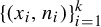 $\{(x_i, n_i)\}_{i=1}^k$
be any finite collection of orbit segments from
 $\mathcal G$
. Since
 $(x_i,n_i)\in \mathcal G$
, Lemma 6.1 gives backward uniform contraction along this ‘good’ orbit: for all
 $y\in B(x_i,\varepsilon )$
and
 $0\le m\le n_i-1$
,
 $$ \begin{align*} d(f^m x_i, f^m y) < C e^{-r(n_i-1-m)}\,d(f^{n_i-1}x_i, f^{n_i-1}y) < C e^{-r(n_i-1-m)}\varepsilon. \end{align*} $$
Thus, the inverse branch of
 $f^{n_i-1}$
that maps back to
 $x_i$
is uniformly contracting on a neighborhood of
 $f^{n_i-1}x_i$
, with contraction rate
 $e^{-r}$
up to a uniform multiplicative constant. In particular,
 $f^{n_i-1}$
maps
 $B_{n_i}(x_i,\varepsilon )$
diffeomorphically onto an open neighborhood of
 $f^{n_i-1}x_i$
that contains the open disk
 $B(f^{n_i-1}x_i,\varepsilon /C)$
.
From the compactness and the strongly topologically mixing property of f, for any
 $\varepsilon>0 $
, there exists some
 $\tau = \tau (\varepsilon ) \in \mathbb {N}$
such that for any open disk
 $B(x,\varepsilon /C)$
, we have
 $f^j(B(x, \varepsilon /C)) = \Lambda $
for some
 $j \leq \tau $
. Hence, for any
 $i = 1, \ldots , k-1$
, we can select
 $\tau _i \leq \tau (\varepsilon )$
such that the image of
 $B(f^{n_i-1} x_i, \varepsilon /C)$
under
 $f^{\tau _i}$
covers
 $B_{n_{i+1}}(x_{i+1}, \varepsilon )$
.
As a consequence of these, we define
 $$ \begin{align*} t_1=0 \quad \text{and} \quad t_j=\sum_{i=1}^{j-1} (n_i-1 + \tau_i) \quad \text{ for } j=2, \ldots, k \end{align*} $$
and set
 $$ \begin{align*} U_1 := B_{n_1}(x_1, \varepsilon). \end{align*} $$
For
 $j=1,\ldots ,k-1$
, define
 $$ \begin{align*} U_{j+1} := \{u\in U_j : f^{t_{j+1}}u \in B_{n_{j+1}}(x_{j+1},\varepsilon)\}. \end{align*} $$
By definition, each
 $U_j$
is open and the family is nested:
 $$ \begin{align*} U_k \subset \cdots \subset U_{j+1} \subset U_j \subset \cdots \subset U_1. \end{align*} $$
We claim that for every
 $j=1,\ldots ,k$
:
-
(1)
$U_j\neq \emptyset $
; -
(2)
$f^{t_j}(U_j)=B_{n_j}(x_j,\varepsilon )$
.


For
 $j=1$
, this is clear, since
 $t_1=0$
and
 $U_1 = B_{n_1}(x_1,\varepsilon )$
.
Assume that items (1) and (2) hold for some
 $1\le j\le k-1$
. Let
 $z\in B_{n_{j+1}}(x_{j+1},\varepsilon )$
be arbitrary. By the choice of
 $\tau _j$
, there exists
 $$ \begin{align*} w \in B (f^{n_j-1}x_j,\varepsilon/C) \subset W_j = f^{n_j-1}(B_{n_j}(x_j,\varepsilon)) \end{align*} $$
such that
 $f^{\tau _j}w = z$
. Since
 $w\in W_j$
, there is a unique
 $y\in B_{n_j}(x_j,\varepsilon )$
with
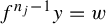 $f^{n_j-1}y = w$
. By the induction hypothesis,
 $f^{t_j}(U_j)=B_{n_j}(x_j,\varepsilon )$
, so we can choose
 $u\in U_j$
with
 $f^{t_j}u = y$
. Then,
 $$ \begin{align*} f^{t_{j+1}}u = f^{t_j+n_j-1+\tau_j}u = f^{\tau_j}w = z\in B_{n_{j+1}}(x_{j+1},\varepsilon), \end{align*} $$
so
 $u\in U_{j+1}$
. Since z was arbitrary, this shows that
 $f^{t_{j+1}}(U_{j+1}) = B_{n_{j+1}}(x_{j+1},\varepsilon )$
and, in particular,
 $U_{j+1}\neq \emptyset $
. This completes the induction.
Thus, all
 $U_j$
are non-empty and
 $$ \begin{align*} U_k \subset \cdots \subset U_2 \subset U_1, \end{align*} $$
so
 $$ \begin{align*} \bigcap_{j=1}^{k} U_j = U_k \neq \emptyset. \end{align*} $$
Choose any
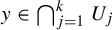 $y \in \bigcap _{j=1}^{k} U_j$
. Then, for every
 $1\le j\le k$
, we have
 $f^{t_j}(y) \in B_{n_j}(x_j,\varepsilon )$
, which is equivalent to
 $$ \begin{align*} d_{n_j}(f^{t_{j}}(y),x_j)<\varepsilon \quad \text{for every }1\le j\le k. \end{align*} $$
Thus, the orbit of
 $y \varepsilon $
-shadows the collection of orbit segments
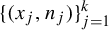 $\{(x_j,n_j)\}_{j=1}^k$
with gaps bounded by
 $\tau (\varepsilon )$
, and
 $\mathcal G$
has specification at scale
 $\varepsilon $
.
6.3 Pressure gap
We prove that if
 $0<r\leq ({c_0}/{3})$
, then for any bounded potential
 $\varphi $
, the ‘bad orbits’ carry less topological pressure than the whole space. Recall we define
 $\psi ^c(x) = \log \|Df|_{E^c(x)}\|$
and
 $$ \begin{align*} \mathcal{S} := \{ (x, n) \in \Lambda \times \mathbb{N} : S_n \psi^c(x) \leq nr \}. \end{align*} $$
We have the following pressure gap estimate.
Theorem 6.3. The collection of bad orbits from the decomposition carries pressure strictly smaller than the topological pressure:
 $$ \begin{align*} P(\mathcal {P} \cup \mathcal {S}, \varphi )< P(\varphi; f ). \end{align*} $$
Proof. We start by taking
 $\mathcal {P} = \emptyset $
. To describe
 $P(\mathcal {S},\varphi )$
, recall we have proven in Lemma 5.3 that
 $$ \begin{align*} \sup_{\mu \in \mathcal{M}_f} \bigg\{ h_{\mu}(f) +\int \varphi \,d\mu: \unicode{x3bb}^c(\mu) \leq \frac{c_0}{3} \bigg\} < P(\varphi; f ). \end{align*} $$
So, for
 $0<r\leq ({c_0}/{3})$
,
 $$ \begin{align} \sup_{\mu \in \mathcal{M}(f)} \bigg\{ h_{\mu}(f) +\int \varphi \,d\mu: \unicode{x3bb}^c(\mu) \leq r \bigg\} < P(\varphi; f ). \end{align} $$
Since we define
 $\psi ^c(x) = \log \| Df|_{E^c(x)} \|$
, for an f-invariant measure
 $\mu $
, its center Lyapunov exponent satisfies
 $\unicode{x3bb} ^c(\mu ) = \int \psi ^c \, d\mu $
.
The left-hand side of (3) can be related to
 $P(\mathcal {S},\varphi )$
. Let
 $E_n \subset \mathcal {S}_n$
be any
 $(n,\varepsilon )$
-separated set. Consider the Borel probability measure
 $$ \begin{align*} \nu_n = \frac{1}{\sum_{x\in E_n}e^{S_n\varphi(x)}}\, \sum_{x\in E_n}\delta_x e^{S_n\varphi(x)}, \quad \mu_n = \frac{1}{n}\sum_{k=0}^{n-1} f_*^k \nu_n. \end{align*} $$
Then, half of the proof of the variational principle (see [Reference WaltersWal82, Theorem 8.6]) shows that if
 $\mu $
is a limit point of
 $\mu _n$
, then
 $\mu $
is f-invariant and satisfies
 $$ \begin{align*} P_{\mu}(\varphi) = h_{\mu}(f) +\int \varphi\, d\mu \geq P(\mathcal{S}, \varphi, \varepsilon). \end{align*} $$
Moreover, by weak
 $^*$
-convergence and the definition of
 $\mathcal {S}$
, we have
 $$ \begin{align*} \unicode{x3bb}^c(\mu) = \int \psi^c \, d\mu \leq r. \end{align*} $$
Combining this with (3), we conclude that
 $$ \begin{align*} P(\mathcal{S}, \varphi) < P(\varphi; f ). \end{align*} $$
Since
 $\mathcal {P} = \emptyset $
, this implies
 $P(\mathcal {P} \cup \mathcal {S}, \varphi ) < P(\varphi; f )$
. By definition,
 $P_{\mathrm {spec}}^{\perp }(\varphi )<P(\varphi; f )$
, which completes the proof.
6.4 Bowen property for potential
Theorem 6.4. Any Hölder continuous potential
 $\varphi $
satisfies the Bowen property on
 $\mathcal {G}$
at scale
 $\varepsilon _0$
.
Proof. Because
 $\varphi $
is Hölder, there exist constants
 $K>0$
and
 $\alpha \in (0,1)$
such that
 $$ \begin{align*} |\varphi(x) - \varphi(y)| \le K\,(d(x,y))^\alpha\quad \text{for all } x,y \in \Lambda. \end{align*} $$
Take
 $(x,n)\in \mathcal {G}$
and
 $y \in B_n(x,\varepsilon )$
. By Lemma 6.1,
 $$ \begin{align*} |S_n \varphi(x) - S_n \varphi(y)| \le K \sum_{k=0}^{n-1} (d(f^k x,\, f^k y))^\alpha < K \sum_{k=0}^{n-1} (Ce^{-r\,(n-1-k)}\,\varepsilon)^\alpha. \end{align*} $$
Re-indexing with
 $j = n-1-k$
and noting the resulting geometric series,
 $$ \begin{align*} K\sum_{k=0}^{n-1}(Ce^{-r(n-1-k)}\,\varepsilon)^\alpha < KC^{\alpha}\,\varepsilon^\alpha\sum_{j=0}^{\infty} e^{-r\,\alpha\,j} < \infty. \end{align*} $$
Hence,
 $|S_n\varphi (x) - S_n\varphi (y)|$
is bounded uniformly in
 $x,n,$
and y, establishing the Bowen property at scale
 $\varepsilon $
.
7 Proof of main theorems
We now complete the proof that if f is a
 $C^3$
-perturbation of
 $f_{\alpha }$
and
 $\varphi :\Lambda \rightarrow {\mathbb {R}}$
, which satisfy the hypotheses of Theorem A, then the conditions of Theorem 2.8 are satisfied and hence there is a unique equilibrium state
 $\mu $
for
 $(\Lambda , f, \varphi )$
. Moreover,
 $\mu $
satisfies the upper level-2 large deviation principle.
By Theorem 5.7,
 $P_{\mathrm {exp}^+}^{\perp }(\varphi ) < P(\varphi; f )$
. We define the decomposition
 $(\mathcal {P}, \mathcal {G}, \mathcal {S})$
as in (1). In Theorem 6.2, we showed that
 $\mathcal {G}$
has specification at all scales. In Theorem 6.4, we showed that
 $\varphi $
has the Bowen property on
 $\mathcal {G}$
. By Theorem 6.3,
 $P(\mathcal {P} \cup \mathcal {S}, \varphi ) < P(\varphi; f )$
. Thus, we see that under the hypotheses of Theorem A, all the hypotheses of Theorem 2.8 are satisfied for the decomposition
 $(\mathcal {P}, \mathcal {G}, \mathcal {S})$
.
Acknowledgments
The author thanks Boris Hasselblatt for invaluable guidance and many helpful discussions. The author is grateful to Vaughn Climenhaga for suggesting this problem and for insightful conversations. The author also thanks the anonymous referee for careful reading and many helpful suggestions that improved the paper.