


1. Introduction
Glacier beds are anisotropic (e.g. Reference Hattestrand, Goodwillie and KlemanHattestrand and others, 1999; personal communication from B. Hubbard, M. J. Siegert and D. McCarroll, 1998), by which is meant that the wavelengths in orthogonal directions are different. This has a number of implications, which are discussed in this paper: (i) velocity and basal-traction vectors are not parallel (Reference NyeNye, 1969; there is some indirect observational evidence for this in East Antarctica, Reference Remy and MinsterRemy and Minster, 1997); (ii) a tensor-type relation must exist between the basal tangential traction and the sliding velocity; (iii) the "invariant" in non-linear sliding laws needs to be generalized. In addition, we discuss: (i) the predictions of Nye-Kamb theory (Reference NyeNye, 1969, Reference Nye1970; Reference KambKamb, 1970) for anisotropic sliding; (ii) the influence of anisotropic beds on surface response and bed-topography-surface-topography relations; and (iii) the influence of anisotropic sliding on large-scale ice-sheet flows.
2. Tensor Sliding Theory
At their simplest, sliding laws relate two vector quantities, the basal tangential traction, Tt, and the basal velocity, u, through a relationship of the form

where the smoothness S is a constant or function relating to the geometry of the bed. These vectors have components (T tx,T ty),(u tx,u ty), respectively. Various generalizations suggest themselves, for example

which includes a non-linear dependence on the norm of the basal traction and the scalar effective pressure pe(e.g. Reference BindschadlerBindschadler, 1983). A functional form for S often used in ice-sheet modelling is

where As is a rate constant.
We now develop the theory for anisotropic beds. It will be seen from section 3 that a consequence of this is that the basal-velocity and basal-traction vectors are not aligned. A familiar analogy of this is the anisotropic permeability of porous media, where the potential gradient (corresponding mathematically to the tangential traction) and the Darcy velocity (corresponding to the sliding velocity) vectors are no longer aligned (Reference BearBear, 1972).
As an example of how an anisotropic bed might arise, let us consider a configuration analogous to that considered by Reference WeertmanWeertman (1957) in his study of sliding. In this analysis, Weertman’s cubic obstructions are replaced by semi-ellipsoids. Suppose that the ice is flowing in a plug flow in a half 3–space with far-field velocity (Ux,Uy,0) and consider a semi-ellipsoid with its flat edge fixed to the base of the half space, aligned with the (x, y, z) frame with principal semi-axes ( lx, ly, lz ) • Strain-rate magnitudes are given by

and a scale estimate of the strain-rate second invariant is  With a Glen rheology

the longitudinal-stress magnitude is

Since we are considering perfect slip, the force, Ft, exerted on the bump acting in the (x, y) directions is given by the appropriate stress times the projected area of the bump normal to the flow, i.e.


and using Equation (2) we find

When considering scale magnitudes we can equate wavenumbers (kx, ky) = (1/lx,1//ly), and can therefore rewrite Equation (5) as

where

and where V=lxlylzR, and R is the number of semi-ellipsoids per unit area.
Relationship (6) exhibits some important points; (i) we expect to see a tensor-relationship between sliding velocity and basal traction; (7) is diagonal simply because we aligned the semi-axes of the ellipsoid with the coordinate frame; (ii) the invariant in the sliding law generalizes to the quadratic form u TKu; (iii) the components of the tensor do not depend upon the velocity field. The general truth of these statements can probably only be verified by numerical computation of ice flow over beds (e.g. Reference GudmundssonGudmundsson, 1997); however, statements (i) and (iii) are also true for Nye-Kamb sliding (see section 3), and in this case as well the tensor components depend upon the square of the wavelength/wavenumber.
We now adopt the italicized parts of statements (i), (ii) and (iii) as constitutive hypotheses and assume that they apply to anisotropic beds in general. The implications of hypothesis (i) is that the smoothness can be written as a tensor S such that

On grounds we shall argue in more detail later, this tensor is diagonalizable, by which we mean that it has real eigenvalues. If the velocity is directed parallel to one of the corresponding eigenvectors, there will be no transverse component to the drag. The eigenvalues are termed the principal smoothnesses and the eigenvectors the principal directions of the smoothness tensor. Equation (6) is expressed in a form where the principal directions of the smoothness tensor are aligned with the coordinate axes; had the semi-ellipsoid not been aligned with the coordinate axes, the R matrix would have been full.
Hypothesis (ii) is of significance because, as we shall shortly see, it creates an invertible form such that we can deduce the drag from the sliding velocity. Hypothesis (iii) is the least likely to be generally true. In the rest of the section we shall suppose that

where m is an exponent; in the previous example and in the Nye-Kamb analysis, we find m = 1.
The inverse form of Relationship (6) can be computed as follows. Writing (6) as

where

we see that we can also write (9) as

and after multiplying the left and right sides by their respective transposes we obtain

where

Substitution of this into Equation (10) gives us L in terms of the traction vector,

and we substitute this into (9) to obtain the inverse form

The scale-model generalization of Equation (1) is thus

where S is the tensor equivalent of S. We shall see in the next section that Nye-Kamb theory gives this functional form for the special case n = 1 and with small bed undulations.
The above argument has supposed that the L and R tensors are diagonal. However, in the above example the diagonal form arises from the fact that we have aligned the axes of the ellipsoid with the coordinate axes. A more general form, where the "grain" of the landscape is not aligned with the coordinate axes, will result in a full smoothness tensor. If we define the principal smoothnesses Si and S2 to be at angle 9 to the coordinate axes, we find the smoothness tensor to be

after applying the usual tensor-transformation rules. For isotropic sliding we can, without loss of generality, take (K, L) = (I, I ), and we then obtain the usual sliding invariant used in glaciology
The quadratic-form construction depends on the existence of the smoothness tensor, and is a form which permits inversion of the sliding relationship, since the forms  and u TKu maintain a constant ratio irrespective of the orientation of the coordinate axes. The dissipation is given by Tt • u = T t • STt, which implies that the tensor S should be positive definite; if it were not energy production could be negative.
Finally, we show that the tensor S is symmetric. A positive-definite matrix is one where the eigenvalues (principal smoothnesses) are positive. This means that we can write S = EAE-1, where A is the diagonal matrix of eigenvalues and E is the matrix of eigenvectors. Since the matrix A is also a smoothness matrix in a rotated frame, by using the usual transformation rules we can write S = RART, where R is the (orthonormal) rotation matrix. This means that the eigenvectors are an orthonormal matrix and we can write S = EAET. This can be written as S = FF T where F = EA1/2. Since the product of a real matrix and its transpose is symmetric, this shows that the smoothness tensor is symmetric.
3. Nye-Kamb Theory
Nye-Kamb theory (Reference NyeNye, 1969, Reference Nye1970; Kamb, Reference Kamb1970) considers the case where a block of ice is moved, with perfect slip, over a flat surface, at aprescribed velocity (Ub, 0, 0). Perturbative undulations in the bed are introduced. These create a first-order velocity field which vanishes at large distance from the surface; the ice velocity therefore remains Ub,0,0,) at large distance. These undulations introduce a drag, which is a second-order quantity as it is a multiple of two first-order quantities, the normal stress and the bed slope. Where slip is perfect, there are no contributions from the second-order stress field to the second-order drag, and we therefore do not need to compute the second-order stress field to compute the second-order drag. We now treat Nye-Kamb sliding over an anisotropic bed. Three-dimensional flow has been treated by Reference NyeNye (1969, Reference Nye1970) who in particular computed the "transverse drag" for the case where the bed-profile autocorrelation function is anisotropic. We consider a simpler case (where two washboards are superimposed), emphasizing the tensorial nature of the solution and the dependence of the tensor components on the components of the wavelength vector; neither of these features are very obvious in Nye’s work. We ignore regelation.
In the rest of the paper we consider perturbed and unperturbed velocity fields. When we are considering a three-dimensional-velocity field, we denote it v with components (vx, vy, vx). Sometimes we wish to restrict consideration to a horizontal-velocity field u which has components (Ux,Uy) = (vx,vy). When we consider this horizontal-velocity-field vector and wish to consider the vertical velocity as well, we denote it w; by definition w = vz.
Now we consider a perturbed half-space  and specifically consider the case
 where μ is a small parameter. In this half-space ice is moving with perfect slip over the base. Following Reference NyeNye (1970) we define a new coordinate
 and obtain the field equations

where ηl is the perturbed three-dimensional vector field, Pl is the perturbed pressure and S is the viscosity of ice. The zeroth-order solution, corresponding to μ = 0, is

Boundary conditions are

where ∇H is the horizontal-divergence operator. (For functions of × and y only, we do not in general distinguish between ∇H and V). These equations possess the solution (cf Reference NyeNye, 1969,Reference Nye1970)

where

Use of the basal kinematical condition shows that

where we have used

and to obtain the average drag per unit area we use the second-order approximation

We can express this in tensor form through

The matrix K has eigenvalues (k • k,0) with corresponding orthogonal principal directions ([kx/ky1],[-ky/kx1]). The orthogonality arises from the symmetry of the matrix. The singularity of the matrix, as evinced by the zero eigenvalue, indicates that we can deduce the drag from the sliding velocity, but that we cannot deduce the sliding velocity from the drag. It stems from the fact that the function exp(−ik · r) is an angled washboard and that the drag parallel to the axis of the washboard must be zero for perfect slip.
In this linear case, more complicated topographies can be constructed by superposing N different washboard topographies. Let us number indices (j,l) ∊(l,N). Use of the basal kinematic condition shows that the normal traction is given by

and the average drag per unit area is given by

where lcm indicates the least common multiple.
A topography containing hummocks and hollows can be created by superposing two washboard topographies defined by wavenumbers (kx,ky) and  which means that the amplitude of the basal topography is
 In this case, we find

This tensor is not singular for non-zero wavenumbers, and can be readily inverted to create the inverse form

Note that the average drag and the zeroth-order velocity are not parallel even in this simple example; this is a result of the additional stresses in the ice caused by the presence of the bed topography. The basic solution of glacier sliding thus gives anisotropic sliding. In this construction we have aligned the principal axes of the sliding tensor with the coordinate axes, but it could equally be aligned with the velocity or the drag. In such a case, the sliding tensor would in general contain non-zero off-diagonal elements. The diagonal form arises from the fact that the washboard axes subtend the same absolute angle with the axes.
Some examples are plotted in Figure 1. The two columns correspond to different basal topography, while the rows correspond to the average drag vector, which is pointed increasingly obliquely to the × axis. In the left column, the wavelength ratios are 2:1, while in the right column, they are 4:1. This will cause the ratio of the principal roughnesses (inverse smoothnesses) to be 4:1 and 16:1 respectively. It can be seen that flow is directed along the longer wavelength direction for relatively small deflections of the drag vector from the × axis, and that this effect is particularly marked for the more anisotropic case. Pressure maxima reside on the upstream side of the bumps, their orientation seeming to be more related to the velocity direction rather than the drag direction.
Anisotropic flow with perfect slip around bumps of wavelength much shorter than the ice thickness (Nye-Kamb configuration). The relationship between basal topography, inter facial-pressure distribution, zeroth-order velocity U0 and the drag vector T2. The two columns correspond to different basal topographies, while the rows correspond to different orientations of the drag vector. These different orientations cause the changing orientation of the velocity vector. If the drag vector were parallel to either of the principal axes of the smoothness tensor, corresponding to the axes of the diagram, the velocity vector would be parallel to the traction vector. Basal topography is indicated by the shape of the lower, grey surface. The pressure is indicated three ways; by the shading on the basal topography, with darker indicating higher presure; by the shape of the upper mesh, and by the three-dimensional contouring on this mesh.

4. Surface Effects
Here we extend to the case of anisotropic sliding analyses due to Reference NyeNye (1959) and to Reference BuddBudd (1970) which show: (i) how disturbances in the surface profile decay to the zeroth order profile; and (h) how variations in the bed profile affect the surface profile. In both cases, we consider flow down an infinitely long and broad plane, with gravity components given by g(ε,0,–1 ). We are assuming ε to be small, but it is not an aspect ratio and not a perturbation parameter. Wavelengths of undulations which give rise to surface effects are much larger than the ice thickness in this analysis and the mechanics can thus be described by the shallow-ice approximation (Reference HutterHutter, 1983). However anisotropic sliding arises from bedrock undulations with wavelength much smaller than the ice thickness so that the effect of these undulations is not noticeable at the surface. We are thus dealing with two distinct limits, one of which gives rise to the surface effects and the other of which gives rise to the anisotropic sliding.
We expand H = H0 + vH× etc., where v is a small parameter. At zeroth order, the basal shear stress is given by

where ρi is the density of ice, g is the acceleration due to gravity and H is the thickness of the ice. There is subtlety here; T0 here refers to the expansion in the small parameter v. This resistance arises from short-wavelength perturbations, and corresponds to the second-order drag T2 obtained from perturbing in parameter μ discussed in section 3.The sliding velocity is given by

(see Equation (8)) where L is the tensor defined in Equation (11). This shows that the zeroth-order velocity need not be in the × direction if the principal smoothnesses are not aligned with the coordinate axes.
The first-order basal tractions are

and the first-order velocity vector becomes

At first order the continuity equation is

To proceed, we define a surface wavenumber ks and write

where we define the scalars

4.1. Decay of surface disturbances
The decay-rate constant is given by the real part of the ratio  which is

We can prove stability as follows. Let us rotate the axes into a coordinate system (x′,y′) determined by the principal directions of L. This implies that the transformed tensor L′ is diagonal, and we can see immediately that the decay rate is

since the principal smoothness  by the positive-definiteness property. The imaginary component can be written
 For one-dimensional flow over an isotropic bed, Ky→0 and without loss of generality we can write L = I, which allows us to retrieve the well-known one-dimensional results.
Wave velocity (i.e. of a washboard surface wave) in the × direction is given by  the × velocity of the plane (washboard wave of opposite orientation to the y axis is given by (Vx+1) U0
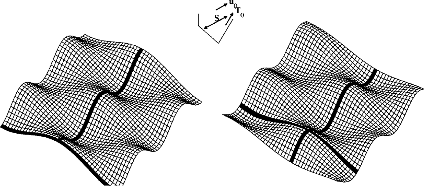
 Both waves will remain plane waves or-Rented at the same angle, moving at different velocities. Since their superposition is hummocks and hollows oriented with the × and y axes, we can anticipate that these features will migrate laterally if Lxy ≠ 0, which of course happens when the principal smoothnesses are not aligned with the coordinate axes/downstream direction. This is illustrated in Figure 2. In particular, we are interested in the ratio of the lateral- and longitudinal-wave-migration velocities, how this relates to the lateral and longitudinal components of the zeroth-order ice-flow velocity and how this wave-velocity ratio is affected by the wavenumbers.
Illustrating the motion of kinematic waves of wavelength greater than the ice thickness. The surface represents the glacier surface and the dark lines are included to demonstrate the wave motion. Note how anisotropic flow leads to lateral wave motion; the lateral velocity depends on the wavelength, i.e. it is dispersive, unlike the downstream velocity.
4.2. Bedrock-surface relationships
We now wish to investigate the steady surface response to bedrock perturbations (Reference HutterHutter, 1983, chapter 4). This is carried out for wavelengths greater than the ice thickness, while the wavelengths which determine the sliding resistance are much less than the ice thickness. We suppose that the bed profile is given by z = b1. The first-order stresses are given by

and the first-order velocity vector becomes

To proceed, we assume the bedrock topography is defined by a wavenumber vector kb and assume that under the linearity assumption this will be the wavelength of the surface topography. Thus,

and we can readily deduce that

and the steady condition is

This equation applies to the case of the angled washboard, i.e. where the bed is a washboard with axes angled to the downstream, × direction. The magnitude of the surface effect is determined by  while
 determines the phasing relative to the bedrock topography.
The superposition of two angled washboards leads to a hummocks and hollows topography, and solution for the elevation may be found by superposing solutions for  Some examples are plotted in Figure 3. The traction vector is aligned with the × axis. The two columns correspond to different basal topography, while the rows correspond to different alignments of the principal smoothnesses, the major one being pointed increasingly obliquely to the × axis. The resulting zeroth-order velocity is indicated. Where the long-wavelength topography (shown on the figure) is anisotropic and aligned orthogonal to the traction direction, surface maxima reside UPsloPe of the basal maxima, but when the long-wavelength basal topography is isotropic, surface maxima reside upflow of the basal maxima. If the sliding were isotropic, upflow and upslope would be in the same direction under the shallow-ice approximation, but anisotropic sliding permits them to be different when the slope and velocity are not aligned with one of the principal axes of the smoothness tensor.
The relationship between basal topography, and ice-surface elevation for wavelengths greater than the ice thickness (the shallow-ice approximation). The two columns correspond to different basal topographies, while the rows correspond to different orientations of the principal smoothnesses. Basal toPgraphy is indicated by the shape of the lower, grey surface. The surface is indicated three ways; by the shading on the basal topography, with darker indicating greater ice-surface elevation; by the shape of the upper mesh; and by the three-dimensional contouring on this mesh. The small axes indicate the direction of the traction (parallel to the × axis), the zeroth-order sliding velocity and the principal smoothnesses. The ratio of principal smoothnesses was 10:1.

4.3. Shock velocities
In valley glaciers, the basic form of the evolution equation for ice thickness is hyperbolic and kinematic waves will form shocks, where there is a jump in the thickness (Reference FowlerFowler, 1982). These shocks will be severely smoothed by diffusion (Reference JohannessonJohannesson, 1992), but the possibility of smoothed shock-like form existing remains. The shock is also of mathematical interest as it represents a limiting non-linear behaviour.
The shock speed v is given by the Rankine-Hugomot condition

where c is the unit vector normal to the shock. If the traction vector is aligned with the × axis, the flux is given by

and the shock speed by

where φ is the angle the shock axis makes with the × axis. The dependence of the shock speed on the angle is thus different for isotropic and anisotropic beds.
5. Applications
5.1. Numerical solutions to the ice-sheet equation
Some calculations based on the European Ice Sheet Modelling Initiative (EISMINT) Benchmark (Reference Huybrechts and PayneHuybrechts and others, 1996) are presented. The basic configuration is a 1500 km2 ice sheet with zero-thickness (Vialov) boundary conditions, which admit a finite outlet flux through zero ice thickness. Accumulation is uniform. Bedrock topography is prescribed (but flat in most of the cases presented here), while flow is not through internal deformation as in the EISMINT Benchmark, but by Weertman sliding and with an anisotropic smoothness tensor using Equation (5). Six calculations are presented and the results are shown in Figure 4.
The influence of bed anisotropy and bed asymmetry on steady ice-sheet profiles computed using the non-linear equations. Based on the EISMIMT Benchmark configuration (Reference Huybrechts and PayneHuybrechts and others, 1996).Sixcalculationsarepresentedascontourplots:(a)flat bed, isotropic smoothness (the EISMIMT Benchmark); (b) flat bed, anisotropic smoothness angled at 0°, principal smoothness ratio of 10:1; ( c) flat bed, anisotropic smoothness angled at 30°, principal smoothness ratio of 10:1; (d) flat bed, anisotropic smoothness angled at 30°, principal smoothness ratio of 2:1; (e) flat bed, anisotropic smoothness angled at 45°, principal smoothness ratio of 10:1; and (f) asymmmetric bed, isotropic smoothness. Bed contours are shown as dotted lines; these can be seen to be asymmetrical about the centre of the solution domain.

Smoothness ratios of 10:1 have a very significant effect, depending on the alignment of the principal directions with the divide ridges. This implies a wavelength ratio of around 3 :1. Smoothness ratios of 2:1 have a less-marked but nevertheless observable effect. Large-scale bed asymmetry has equally marked, but qualitatively different effects.
5.2. Rugose topography underlying cold-based ice sheets
Cold-based ice sheets contain a shear layer at the base (Reference FowlerFowler, 1992) where most of the internal deformation occurs. This layer arises because the basal viscosity is lower owing to the higher stresses and temperatures. Rugose topography which substantially penetrates this layer is likely to affect the flow of ice sheets. If this topography has a grain, then cold-based ice is also likely to exhibit non-parallelism between surface slopes and flow directions. Such non-parallelism should not be used a priori to infer either warm bases or the breakdown of the shallow-ice approximation.
6. Conclusions
-
(1) Anisotropic beds give rise to non-parallel basal-tangential-traction and basal-sliding vectors, which are related by a smoothness tensor. This tensor is real and symmetric to ensure positive definiteness, necessary on account of the Second Law of Thermodynamics. This tensor can be diagonalized, with the two eigenvalues, necessarily both positive, called the principal major and principal minor smoothnesses. In the shallow-ice approximation, velocity and slope vectors are no longer parallel in general, which means that there is a distinction between upslope when considering the ice surface and upflow Non-linear sliding requires a generalization of the absolute value of the slope in terms of a quadratic form involving the slope vector and the inverse smoothness tensor.
-
(2) The Nye-Kamb solution for short-wavelength obstructions predicts anisotropic sliding, with the strengths of the principal smoothnesses being proportional to the wavelength squared for linear rheologies. For wavelength ratios of 4:1, tractions deviating only slightly from the direction of the minor principal smoothness result in velocities strongly aligned with the major principal smoothness.
-
(3) For flow according to the shallow-ice approximation down the infinite plane, the decay rate of surface disturbances is given by
 Plane wave velocities in the × direction are given by Plane waves of opposite orientation(e.g. with ky of opposite sign) have a different wave velocity, which means that superpositions of these plane waves, which are hummocks and hollows, have lateral velocities which depend on the relative wavelength and the orientation of the principal smoothnesses.
-
(4) Under steady flow, according to the shallow-ice approximation, steady anisotropic sliding can affect surface-topography-basal-topography relationships. If the long-wavelength basal topography is of shorter wavelength in the direction of the traction vector, then the ice-surface highs are found upslope of the basal highs. If the long-wavelength basal topography is isotropic, ice-surface highs reside upflow of the basal highs.
-
(5) Shock waves angled at 9 across the direction of flow have a shock-wave velocity cos 9 of that of a wave with axis orthogonal to the flow when sliding is isotropic. Anisotropic sliding will cause there to be a different relationship between the angle subtended by the axis of a plane shock wave and the direction of maximum of slope.
-
(6) Anisotropic sliding causes deflection of divide ridges compared with the isotropic case. This may be of significance in East Antarctica, where basal temperatures in central regions reach melting point.
-
(7) Anisotropic sliding will make inferring the deposition location of snow in off-divide cores more difficult; slope strike does not equal flow strike.
 Plane wave velocities in the × direction are given by
 Plane waves of opposite orientation(e.g. with ky of opposite sign) have a different wave velocity, which means that superpositions of these plane waves, which are hummocks and hollows, have lateral velocities which depend on the relative wavelength and the orientation of the principal smoothnesses.
Acknowledgements
Thanks to G. H. Gudmundsson and K. Hutter for their careful reviewing.



