1 Introduction
Several studies have been devoted to the stability of a columnar vertical vortex in stably stratified fluids. Axisymmetric columnar vortices can be unstable to centrifugal instability when the Rayleigh discriminant is negative (Smyth & McWilliams Reference Smyth and Mcwilliams1998; Billant & Gallaire Reference Billant and Gallaire2005). Shear instability may also occur when the vorticity gradient vanishes at some radius (Rayleigh Reference Rayleigh1880) since it is a two-dimensional instability. In addition, the vortex can spontaneously radiate internal waves owing to an over-reflection mechanism (Smyth & McWilliams Reference Smyth and Mcwilliams1998; Billant & Le Dizès Reference Billant and Le Dizès2009; Le Dizès & Billant Reference Le Dizès and Billant2009; Riedinger, Le Dizès & Meunier Reference Riedinger, Le Dizès and Meunier2010). However, many studies have shown that vortices have a pancake or lenticular shape in stratified fluids rather than being columnar. For example, interacting columnar vortices are unstable to zigzag instability (Billant & Chomaz Reference Billant and Chomaz2000; Otheguy, Chomaz & Billant Reference Otheguy, Chomaz and Billant2006; Billant Reference Billant2010; Billant et al.
Reference Billant, Deloncle, Chomaz and Otheguy2010; Deloncle, Billant & Chomaz Reference Deloncle, Billant and Chomaz2011) and evolve into pancake vortices with a small aspect ratio. Coherent vortices generated from wakes or turbulence in stratified fluids also have a pancake shape (Lin, Boyer & Fernando Reference Lin, Boyer and Fernando1992; Chomaz et al.
Reference Chomaz, Bonneton, Butet and Hopfinger1993; Fincham, Maxworthy & Spedding Reference Fincham, Maxworthy and Spedding1996; Spedding, Browand & Fincham Reference Spedding, Browand and Fincham1996; Bonnier, Eiff & Bonneton Reference Bonnier, Eiff and Bonneton2000). In laboratory experiments, pancake vortices can be directly generated by different devices, imposing a rotation to a layer of fluid (Flór & van Heijst Reference Flór and van Heijst1996; Beckers et al.
Reference Beckers, Verzicco, Clercx and van Heijst2001). Many pancake vortices are also observed in oceans. Famous examples are the Mediterranean eddies (Meddies) which are formed by salty water flowing from the Mediterranean sea into the mid-Atlantic ocean (Armi et al.
Reference Armi, Hebert, Oakey, Price, Richardson, Rossby and Ruddick1989; Hobbs Reference Hobbs2007; Ménesguen et al.
Reference Ménesguen, Hua, Carton, Klingelhoefer, Schnrle and Reichert2012). Meddies typically have a horizontal extension of
 $O(100)~\text{km}$
and vertical thickness of
 $O(1)~\text{km}$
(Richardson, Bower & Zenk Reference Richardson, Bower and Zenk2000). For these vortices, planetary rotation has an important effect, in addition to the stable stratification, but this effect will not be considered in the present paper.
Despite the ubiquity of pancake vortices in stratified fluids, only a few studies on their structure and stability exist. The internal structure of a pancake vortex in stably stratified fluids has been investigated by Flór & van Heijst (Reference Flór and van Heijst1996), Bonnier et al. (Reference Bonnier, Eiff and Bonneton2000) and Beckers et al. (Reference Beckers, Verzicco, Clercx and van Heijst2001). Flór & van Heijst (Reference Flór and van Heijst1996) conducted an experimental study on monopolar pancake vortices using three different generation methods (rotating sphere, rotating rod and injection of fluids). They found that disturbances with azimuthal wavenumber
 $m=2$
or
 $m=3$
are unstable when the Froude number
 $F=V_{max}/NR_{vmax}$
is larger than
 $F>0.1$
, where
 $V_{max}$
is the maximum azimuthal velocity,
 $N$
the Brunt–Väisälä frequency and
 $R_{vmax}$
the radius of maximum azimuthal velocity. They also showed that the nonlinear evolution of the instabilities (formations of tripole (
 $m=2$
) and dipole splitting) is similar to that of two-dimensional vortices. Some differences come from the faster decay rate of the satellites compared to the core for pancake vortices. Bonnier et al. (Reference Bonnier, Eiff and Bonneton2000) investigated experimentally the dynamics of vortices in the far wake of a towed sphere. The density field inside the vortices shows a pinching of the isopycnals in order to satisfy the hydrostatic and cyclostrophic balances. Beckers et al. (Reference Beckers, Verzicco, Clercx and van Heijst2001) found similar isopycnal deformations experimentally and numerically. They have shown that, when the vortex is not initially in cyclostrophic or hydrostatic balance, adjustment processes occur and lead to the generation of internal gravity waves. A Kirchhoff elliptic pancake vortex in cyclostrophic balance also emits gravity waves (Plougonven & Zeitlin Reference Plougonven and Zeitlin2002). Balanced vortices exhibit particular momentum and density diffusions. Beckers et al. (Reference Beckers, Verzicco, Clercx and van Heijst2001) and Godoy-Diana & Chomaz (Reference Godoy-Diana and Chomaz2003) have studied the effect of the Schmidt number
 $Sc={\it\nu}/{\it\kappa}$
, which is the ratio of the diffusion rates of momentum
 ${\it\nu}$
and density
 ${\it\kappa}$
. When
 $Sc\gg 1$
, secondary circulations slow down the decay of the vortex. In contrast, when
 $Sc<1$
, these secondary circulations accelerate the decay of the vortex.
The stability of a pancake vortex as a function of Reynolds number and Froude number is discussed in Beckers et al. (Reference Beckers, Clercx, van Heijst and Verzicco2003) experimentally and numerically for a vortex profile with angular velocity
 ${\it\Omega}={\it\Omega}_{0}\exp (-(r/R)^{q}-(z/{\it\Lambda})^{2})$
, where
 ${\it\Omega}_{0}$
is the maximum angular velocity,
 $q$
the steepness parameter,
 $R$
the radius and
 ${\it\Lambda}$
the thickness. Beckers et al. (Reference Beckers, Clercx, van Heijst and Verzicco2003) have determined only the most unstable modes by performing nonlinear numerical simulations of azimuthally perturbed vortices using the Navier–Stokes equations under the Boussinesq approximation. They focused on perturbations with azimuthal wavenumbers
 $m\geqslant 2$
with a Reynolds number up to
 $\tilde{Re}=10^{4}$
where
 $\tilde{Re}=2\sqrt{{\rm\pi}}{\it\Lambda}R{\it\Omega}_{0}/{\it\nu}$
. They have shown that pancake vortices with an aspect ratio fixed to
 ${\it\alpha}={\it\Lambda}/R=0.4$
with
 $q>2$
are generally unstable to barotropic (i.e. shear) instability in the ranges of
 $500\leqslant \tilde{Re}\leqslant 10^{4}$
and
 $0.1\leqslant \tilde{F}\leqslant 0.8$
, where the Froude number is defined as
 $\tilde{F}=2\sqrt{{\rm\pi}}{\it\Lambda}{\it\Omega}_{0}/(RN)$
. The instability is similar to shear instability of two-dimensional vortices with the most unstable azimuthal wavenumber increasing with the steepness parameter
 $q$
(Carton & Legras Reference Carton and Legras1994). When
 $q=2$
, they found that the vortex is stable.
Recently, Negretti & Billant (Reference Negretti and Billant2013) have conducted a linear stability analysis of a pancake vortex with a Gaussian vertical vorticity profile in the radial and vertical directions. They found that the vortex is unstable to gravitational instability when the vortex aspect ratio
 ${\it\alpha}$
is small such that
 ${\it\alpha}/F_{h}<1.1$
, where
 $F_{h}={\it\Omega}_{0}/N$
. When this condition is satisfied, the isopycnals are indeed so deformed by the pancake shape that they overturn. The barotropic shear instability does not exist because the vorticity gradient does not vanish for a Gaussian vertical vorticity profile. They have also shown that the vertical shear is never sufficient to trigger an instability when
 ${\it\alpha}/F_{h}>1.1$
.
In this paper, we investigate the stability of an axisymmetric pancake vortex with the same angular velocity profile as in Beckers et al. (Reference Beckers, Clercx, van Heijst and Verzicco2003) in a stably stratified fluid. The steepness parameter will be set to
 $q=2$
throughout the paper. In contrast to Beckers et al. (Reference Beckers, Clercx, van Heijst and Verzicco2003), all the unstable modes will be determined by solving the eigenvalue problem by means of an iterative method. The Reynolds number will be increased up to
 $Re\equiv {\it\Omega}_{0}R^{2}/{\it\nu}=10^{5}$
and various aspect ratios and Froude numbers will be studied. We have found that the vortex can be also unstable under some conditions to the
 $m=2$
shear instability when
 $q=2$
. In addition, we will show that other types of instability exist: the counterpart of the centrifugal instability of columnar vortices and two instabilities specific to pancake vortices. The latter constitute the gravitational instability, already extensively studied by Negretti & Billant (Reference Negretti and Billant2013), and the baroclinic instability that has not been observed before in purely stratified fluids.
The paper is organized as follows: we first define the linear stability problem in § 2. In § 3, typical spectra and eigenmodes for the azimuthal wavenumbers
 $m=0,1,$
and
 $2$
will be presented. The origin of the different modes will be identified thanks to stability criteria and by comparison to the instabilities of columnar vortices. In § 4, a parametric study of the most unstable modes for each
 $m$
will then be conducted as a function of the aspect ratio, Froude and Reynolds numbers. From the fact that centrifugal and shear instabilities in pancake and columnar vortices have many resemblances, we further show in §§ 5 and 6 that their occurrence in pancake vortices can be understood from their growth rate dependence with the vertical wavenumber in columnar vortices. The instabilities specific to pancake vortices will be discussed in § 7. Finally, all the different instabilities for each azimuthal wavenumber
 $m$
are summarized in § 8 in the parameter space: Froude number and Reynolds number for
 $Re\leqslant 10^{4}$
. In § 9, comparisons to previous experimental and numerical studies are presented.
2 Problem formulation
2.1 The base state
We consider as the base flow an axisymmetric pancake vortex with only azimuthal velocity
 $\boldsymbol{u}_{b}(r,{\it\theta},z)=[u_{br},u_{b{\it\theta}},u_{bz}]=[0,r{\it\Omega}(r,z),0]$
in cylindrical coordinates (
 $r,{\it\theta},z$
). The angular velocity is chosen to be Gaussian in both the radial and vertical directions
 $$\begin{eqnarray}\displaystyle {\it\Omega}(r,z)={\it\Omega}_{0}\text{e}^{-(r^{2}/R^{2}+z^{2}/{\it\Lambda}^{2})}, & & \displaystyle\end{eqnarray}$$
where
 $R$
is the radius,
 ${\it\Lambda}$
is the half-thickness and
 ${\it\Omega}_{0}$
is the maximum angular velocity. The total pressure and density are decomposed as follows:
 $$\begin{eqnarray}\displaystyle & \displaystyle p_{t}=p_{0}+\bar{p}(z)+p_{b}(r,z), & \displaystyle\end{eqnarray}$$
 $$\begin{eqnarray}\displaystyle & \displaystyle {\it\rho}_{t}={\it\rho}_{0}+\bar{{\it\rho}}(z)+{\it\rho}_{b}(r,z), & \displaystyle\end{eqnarray}$$
 $0$
are reference values, those with a bar indicate the background vertical profiles and those with a subscript
 $b$
correspond to the perturbations due to the base vortex. The Euler equations under the Boussinesq approximation in the radial and vertical directions are
 $$\begin{eqnarray}\displaystyle & \displaystyle -r{\it\Omega}^{2}=-\frac{1}{{\it\rho}_{0}}\frac{\partial p_{t}}{\partial r}, & \displaystyle\end{eqnarray}$$
 $$\begin{eqnarray}\displaystyle & \displaystyle \frac{g}{{\it\rho}_{0}}{\it\rho}_{t}=-\frac{1}{{\it\rho}_{0}}\frac{\partial p_{t}}{\partial z}, & \displaystyle\end{eqnarray}$$
 $g$
is the gravity. Combining (2.4) and (2.5) gives the thermal wind relation:
 $$\begin{eqnarray}\displaystyle \frac{\partial r{\it\Omega}^{2}}{\partial z}=-\frac{g}{{\it\rho}_{0}}\frac{\partial {\it\rho}_{b}}{\partial r}. & & \displaystyle\end{eqnarray}$$
Hence,
 ${\it\rho}_{b}$
is given by
 $$\begin{eqnarray}\displaystyle {\it\rho}_{b}(r,z)=-z\frac{{\it\rho}_{0}}{g}\left(\frac{R}{{\it\Lambda}}\right)^{2}{\it\Omega}_{0}^{2}\text{e}^{-2(r^{2}/R^{2}+z^{2}/{\it\Lambda}^{2})}. & & \displaystyle\end{eqnarray}$$
2.2 Linearized equations
The vortex is perturbed by infinitesimal perturbations (denoted with a prime) of velocity
 $\boldsymbol{u}^{\prime }=[u_{r}^{\prime },u_{{\it\theta}}^{\prime },u_{z}^{\prime }]$
, pressure
 $p^{\prime }$
and density
 ${\it\rho}^{\prime }$
according to
 $$\begin{eqnarray}\displaystyle & \displaystyle \boldsymbol{u}(r,{\it\theta},z)=\boldsymbol{u}_{b}+\boldsymbol{u}^{\prime }=(0,r{\it\Omega}(r,z),0)+(u_{r}^{\prime },u_{{\it\theta}}^{\prime },u_{z}^{\prime }), & \displaystyle\end{eqnarray}$$
 $$\begin{eqnarray}\displaystyle & \displaystyle p=p_{t}+p^{\prime }, & \displaystyle\end{eqnarray}$$
 $$\begin{eqnarray}\displaystyle & \displaystyle {\it\rho}={\it\rho}_{t}+{\it\rho}^{\prime }. & \displaystyle\end{eqnarray}$$
 $$\begin{eqnarray}\displaystyle [u_{r}^{\prime },u_{{\it\theta}}^{\prime },u_{z}^{\prime },p^{\prime },{\it\rho}^{\prime }]=\left[u_{r}(r,z),u_{{\it\theta}}(r,z),u_{z}(r,z),{\it\rho}_{0}p(r,z),\frac{{\it\rho}_{0}}{g}{\it\rho}(r,z)\right]\text{e}^{-\text{i}{\it\omega}t+\text{i}m{\it\theta}}+\text{c.c}., & & \displaystyle \nonumber\\ \displaystyle & & \displaystyle\end{eqnarray}$$
where
 ${\it\omega}$
is the frequency and
 $m$
the azimuthal wavenumber. We consider that
 $m$
is positive since negative wavenumbers can be recovered by the symmetry:
 ${\it\omega}(m)={\it\omega}^{\ast }(-m)$
. Under the Boussinesq approximations, the linearized Navier–Stokes equations are
 $$\begin{eqnarray}\displaystyle & \displaystyle -\text{i}({\it\omega}-m{\it\Omega})u_{r}-2{\it\Omega}u_{{\it\theta}}=-\frac{\partial p}{\partial r}+{\it\nu}\left({\rm\nabla}^{2}u_{r}-\frac{1}{r^{2}}u_{r}-\frac{2}{r^{2}}\text{i}mu_{{\it\theta}}\right) & \displaystyle\end{eqnarray}$$
 $$\begin{eqnarray}\displaystyle & \displaystyle -\text{i}({\it\omega}-m{\it\Omega})u_{{\it\theta}}+{\it\zeta}u_{r}+\frac{\partial r{\it\Omega}}{\partial z}u_{z}=-\frac{\text{i}m}{r}p+{\it\nu}\left({\rm\nabla}^{2}u_{{\it\theta}}-\frac{1}{r^{2}}u_{{\it\theta}}+\frac{2}{r^{2}}\text{i}mu_{r}\right) & \displaystyle\end{eqnarray}$$
 $$\begin{eqnarray}\displaystyle & \displaystyle -\text{i}({\it\omega}-m{\it\Omega})u_{z}=-\frac{\partial p}{\partial z}-{\it\rho}+{\it\nu}{\rm\nabla}^{2}u_{z} & \displaystyle\end{eqnarray}$$
 $$\begin{eqnarray}\displaystyle & \displaystyle -\text{i}({\it\omega}-m{\it\Omega}){\it\rho}+\frac{g}{{\it\rho}_{0}}\frac{\partial {\it\rho}_{b}}{\partial r}u_{r}+\frac{g}{{\it\rho}_{0}}\frac{\partial {\it\rho}_{b}}{\partial z}u_{z}=N^{2}u_{z}+{\it\kappa}{\rm\nabla}^{2}{\it\rho} & \displaystyle\end{eqnarray}$$
 $$\begin{eqnarray}\displaystyle & \displaystyle \frac{1}{r}\frac{\partial ru_{r}}{\partial r}+\frac{1}{r}\text{i}mu_{{\it\theta}}+\frac{\partial u_{z}}{\partial z}=0, & \displaystyle\end{eqnarray}$$
 ${\it\zeta}=1/r\partial (r^{2}{\it\Omega})/\partial r$
is the vertical vorticity,
 $N=\sqrt{-g/{\it\rho}_{0}\text{d}\bar{{\it\rho}}/\text{d}z}$
the Brunt–Väisälä frequency which is assumed constant,
 ${\it\nu}$
the viscosity and
 ${\it\kappa}$
the diffusivity of the stratifying agent. The viscous and diffusive damping of the base state are neglected in (2.12)–(2.16). This classical assumption in stability analyses is valid as long as the growth rate of the instabilities is large enough compared to the viscous and diffusive decay of the base state (Drazin & Reid Reference Drazin and Reid1981). The problem is governed by four non-dimensional numbers: aspect ratio (
 ${\it\alpha}$
), Froude number (
 $F_{h}$
), Reynolds number (
 $Re$
) and Schmidt number (
 $Sc$
), defined as follows:
 $$\begin{eqnarray}\displaystyle {\it\alpha}=\frac{{\it\Lambda}}{R},\quad F_{h}=\frac{{\it\Omega}_{0}}{N},\quad Re=\frac{{\it\Omega}_{0}R^{2}}{{\it\nu}},\quad Sc=\frac{{\it\nu}}{{\it\kappa}}. & & \displaystyle\end{eqnarray}$$
In most of the paper, we keep
 $Sc=1$
for simplicity. Nevertheless, the effect of the Schmidt number will be briefly investigated in § 4.4.
2.3 Numerical method
Equations (2.12)–(2.16) are discretized with a finite element method using FreeFem
 $++$
(Garnaud Reference Garnaud2012; Hecht Reference Hecht2012; Garnaud et al.
Reference Garnaud, Lesshafft, Schmid and Huerre2013). Velocity, density and pressure
 $(\boldsymbol{u},{\it\rho},p)$
are approximated with (P2, P1, P1) triangular elements (also known as Taylor–Hood elements), respectively (Elman, Silvester & Wathen Reference Elman, Silvester and Wathen2005; Hecht Reference Hecht2012; De Vuyst Reference De Vuyst2013). The mesh is adapted to the base state and refined around the vortex core. The domain is restricted to positive radius
 $r=[0,R_{max}]$
and is set to
 $z=[-Z_{max},Z_{max}]$
along the vertical. The boundary conditions at
 $r=0$
differ depending on the azimuthal wavenumber
 $m$
(Batchelor & Gill Reference Batchelor and Gill1962; Ash & Khorrami Reference Ash, Khorrami and Green1995),
 $$\begin{eqnarray}\displaystyle \left.\begin{array}{@{}l@{}}m=0:\quad u_{r}=u_{{\it\theta}}=0,\\ m=1:\quad u_{z}=p={\it\rho}=0,\\ m\geqslant 2:\quad u_{r}=u_{{\it\theta}}=u_{z}=p={\it\rho}=0.\end{array}\right\} & & \displaystyle\end{eqnarray}$$
At the other boundaries
 $r=R_{max}$
and
 $z=\pm Z_{max}$
, all perturbations are enforced to vanish.
Growth rate for different domain sizes
 $R_{max}$
and
 $Z_{max}$
for
 $m=2$
,
 ${\it\alpha}=0.5$
,
 $F_{h}=0.5$
and
 $Re=10^{4}$
for mesh sizes
 $S_{max}=0.075R$
and
 $S_{min}=0.004R$
.

The resulting discretized equations (2.12)–(2.16) are written in the form
 $$\begin{eqnarray}\displaystyle -\text{i}{\it\omega}\unicode[STIX]{x1D63D}\boldsymbol{v}=\unicode[STIX]{x1D647}\boldsymbol{v}, & & \displaystyle\end{eqnarray}$$
where
 $\boldsymbol{v}=[u_{r},u_{{\it\theta}},u_{z},p,{\it\rho}]$
. The typical size of the matrices
 $\unicode[STIX]{x1D63D}$
and
 $\unicode[STIX]{x1D647}$
is approximately
 $10^{6}\times 10^{6}$
. The generalized eigenvalue problem (2.19) is solved with an iterative Krylov–Schur method using the libraries SLEPc and PETSc (Hernandez, Roman & Vidal Reference Hernandez, Roman and Vidal2005; Garnaud Reference Garnaud2012; Garnaud et al.
Reference Garnaud, Lesshafft, Schmid and Huerre2013; Balay et al.
Reference Balay, Abhyankar, Adams, Brown, Brune, Buschelman, Eijkhout, Gropp, Kaushik and Knepley2014). The shift-invert spectral transformation is used to find the most unstable eigenvalues/vectors around shift values. Spurious modes are eliminated by excluding eigenvalues varying by more than
 $10^{-6}$
between two successive shift values.
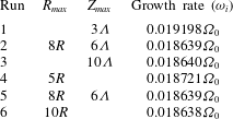
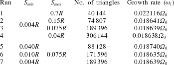
Tables 1 and 2 show examples of the convergence of the growth rate as a function of the domain size (
 $R_{max},Z_{max}$
) and mesh size, respectively. Table 1 shows that there is only a relative variation of 0.005 % of the growth rate when
 $R_{max}$
is increased from
 $8R$
to
 $10R$
or when
 $Z_{max}$
is increased from
 $6{\it\Lambda}$
to
 $10{\it\Lambda}$
. As seen in table 2, the growth rate varies significantly when the maximum mesh size is varied from
 $0.7R$
to
 $0.15R$
(see runs 1 and 2) but becomes almost constant when
 $S_{max}$
is smaller than
 $0.15R$
(see runs 2 to 4). In turn, when the maximum mesh size is fixed to
 $S_{max}=0.075R$
, the growth rate varies very little when the minimum mesh size
 $S_{min}$
is lower than
 $0.01R$
(see runs 6 to 7). The mesh adaptation to the base vortex allows us to use sufficiently fine meshes in the vortex core while keeping a reasonable total number of triangles. In the following, the numerical results are mostly computed for a domain size
 $R_{max}=8R$
and
 $Z_{max}=6{\it\Lambda}$
and for a mesh with a maximum size
 $0.075R$
and minimum size
 $0.004R$
(runs 3 or 7).
Growth rate for different minimum and maximum mesh sizes
 $S_{min}$
and
 $S_{max}$
for
 $m=2$
,
 ${\it\alpha}=0.5$
,
 $F_{h}=0.5$
and
 $Re=10^{4}$
for
 $R_{max}=8R$
and
 $Z_{max}=6{\it\Lambda}$
. The number of triangles is also indicated.

For comparison purposes we have also conducted some stability analyses of a columnar vortex with base angular velocity
 ${\it\Omega}=\exp (-r^{2})$
. The vertical dependence of the perturbations can then be expressed in terms of normal modes with a vertical wavenumber
 $k$
. Equations (2.12)–(2.16) have been solved by means of a Chebyshev pseudospectral collocation method (Antkowiak & Brancher Reference Antkowiak and Brancher2004; Fabre & Jacquin Reference Fabre and Jacquin2004). An algebraic mapping and 320 collocation points have been used. The numerical code based on FreeFem
 $++$
and SLEPc for
 ${\it\alpha}\rightarrow \infty$
has also been successfully checked against the Chebyshev code. For example, for
 $m=1,F_{h}=0.5$
and
 $Re=10^{4}$
, the maximum growth rates obtained by these two codes are
 ${\it\omega}/{\it\Omega}_{0}=0.149+0.143\text{i}$
and
 ${\it\omega}/{\it\Omega}_{0}=0.148+0.144\text{i}$
, respectively.
3 Some typical examples of spectra
In this section, we show typical examples of the spectra and eigenmodes for the different azimuthal wavenumbers
 $m=0$
, 1 and 2. The Reynolds number is fixed to
 $Re=10^{4}$
but the Froude number and aspect ratio are varied from one azimuthal wavenumber to the other in order to show the most general spectrum for each
 $m$
. To identify the instability, the spectra are compared to the corresponding spectra of a columnar vortex for the same control parameters (
 $F_{h},Re$
). Detailed comparisons between the eigenmodes of columnar and pancake vortices are also carried out.
3.1
 $m=0$

Figure 1 shows an example of the spectrum for the parameters
 $m=0$
,
 ${\it\alpha}=1$
,
 $F_{h}=0.5$
and
 $Re=10^{4}$
. The frequency (
 ${\it\omega}_{r}$
) and growth rate (
 ${\it\omega}_{i}$
) are non-dimensionalized by the maximum angular velocity
 ${\it\Omega}_{0}$
. The unstable mode are displayed by symbols and are labelled (
 $m,i$
) where
 $i$
denotes the
 $i$
th mode. For each point, there are actually two modes with a different symmetry with respect to
 $z=0$
: symmetric (○) and antisymmetric (

 $(u_{r})$
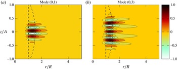
of the most unstable antisymmetric mode (marked (0,1) in figure 1) is depicted in figure 2(a). The perturbation lies at the periphery of the vortex core
 $r/R\geqslant 1$
and in the central region
 $-0.5\leqslant z/{\it\Lambda}\leqslant 0.5$
along the vertical. A well-defined axial wavelength at
 ${\it\lambda}\simeq 0.2{\it\Lambda}$
can be seen. The symmetric mode marked as (0,3) (figure 2
b) is similar to the mode (0,1) but with a larger extent in the vertical direction
 $-0.7\leqslant z/{\it\Lambda}\leqslant 0.7$
with a slightly smaller wavelength
 ${\it\lambda}\simeq 0.17{\it\Lambda}$
. The other modes (0,2), (0,4) and (0,5) have similar characteristics to these two modes: they only differ by the number of nodes along the vertical.
Growth rate (
 ${\it\omega}_{i}/{\it\Omega}_{0}$
) and frequency (
 ${\it\omega}_{r}/{\it\Omega}_{0}$
) spectra for a pancake vortex (
 ${\it\alpha}=1$
) (○: for symmetric and

 ${\it\alpha}=\infty$
) (

 $m=0$
,
 $F_{h}=0.5$
, and
 $Re=10^{4}$
. The mode (C,0) corresponds to the most unstable mode of the columnar vortex.

Real part of the radial velocity perturbation Re(
 $u_{r}$
) of (a) antisymmetric mode (0,1) and (b) symmetric mode (0,3) of figure 1. The radius
 $r$
and height
 $z$
are rescaled with the radius
 $R$
and half-height
 ${\it\Lambda}$
of the base vortex, respectively. The dashed line represents the contour where the Rayleigh discriminant
 ${\it\Phi}$
vanishes. The dotted line indicates the contour where the angular velocity
 ${\it\Omega}$
of the base vortex is
 $0.1{\it\Omega}_{0}$
.

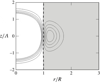
To determine the origin of this instability, we consider the Rayleigh criterion for centrifugal instability extended to baroclinic vortices (Solberg Reference Solberg1936; Eliassen & Kleinschmidt Jr Reference Eliassen, Kleinschmidt and Bartels1957). Centrifugal instability is expected when the circulation decreases with the radius along isopycnal surfaces
 $$\begin{eqnarray}\displaystyle {\it\Phi}=\left.\frac{1}{r^{3}}\frac{\partial (r^{2}{\it\Omega})^{2}}{\partial r}\right|_{{\it\rho}_{t}}<0, & & \displaystyle\end{eqnarray}$$
for some radius. The region where
 ${\it\Phi}$
is negative for
 ${\it\alpha}=1,F_{h}=0.5$
is shaded in figure 3. It extends from
 $r=1$
to infinity with a minimum of
 ${\it\Phi}$
reached near
 $r=1.2R$
and
 $z=0$
. As shown by the dashed lines in figure 2, the modes are localized in this region. This shows that these modes are due to centrifugal instability. In order to further understand their properties, the spectrum of a columnar vortex (
 ${\it\alpha}=\infty$
) has been computed for the same parameters (
 $m=0,F_{h}=0.5$
,
 $Re=10^{4}$
). It is plotted in figure 1 as a grey continuous line. Although the spectrum is discretized for
 ${\it\alpha}=1$
and continuous for
 ${\it\alpha}=\infty$
, since the vertical wavenumber varies continuously, the maximum growth rate in both cases is very close but it is slightly smaller for pancake vortices. Note that there exists a single unstable mode for each wavenumber in the columnar case. The secondary centrifugal modes with more radial oscillations become unstable only for larger Froude or Reynolds numbers. Furthermore, their growth rates are much smaller than the primary modes both for columnar and pancake vortices.
Contours of
 ${\it\Phi}/|{\it\Phi}_{min}|$
for
 ${\it\alpha}=1,F_{h}=0.5$
. The regions where
 ${\it\Phi}$
is negative are shaded. The contour interval is
 $0.2$
.

3.2
$m=1$

The symbols in figure 4 show a typical example of the spectrum for
 $m=1,{\it\alpha}=0.5$
,
 $F_{h}=1/3$
and
 $Re=10^{4}$
. Several unstable modes exist (labelled (1,1)–(1,7) using the same notation as for
 $m=0$
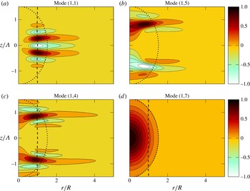
). This time, all modes have non-zero frequency. Figure 5(a) shows the real part of the radial velocity of the most unstable mode (1,1). The mode is maximum near
 $r/R=1$
and localized within
 $-1<z/{\it\Lambda}<1$
with a typical wavelength
 ${\it\lambda}\simeq 0.57{\it\Lambda}$
. It resembles the
 $m=0$
centrifugal modes (figure 2) except that the perturbations overshoot in the region of positive generalized Rayleigh discriminant. The modes (1,2) and (1,3) are similar to the mode (1,1) except that they exhibit more oscillations along the vertical. In contrast, the mode (1,5) is different (figure 5
b): the perturbation is localized within the vortex core
 $r/R<1$
and maximum near
 $z=\pm {\it\Lambda}$
. The perturbation is mainly located in a region where
 ${\it\Phi}$
is positive and is therefore probably not a centrifugal mode.
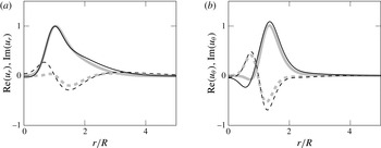
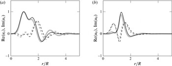
To identify this instability, it is useful to compare the spectrum to one of a columnar vortex with the same parameters (shown by a thick line in figure 4). The growth rate for a columnar vortex first increases with frequency and then decreases owing to viscous stabilization since the corresponding vertical wavenumber is large. The maximum growth rate is slightly higher than for the pancake vortex. Figure 6(a,b) compare the radial profiles of the horizontal velocity (
 $u_{r},u_{{\it\theta}}$
) of the most unstable modes of the pancake and columnar vortices (labelled (1,1) and (C,1,1) in figure 4, respectively). The profiles for the pancake vortex are taken at the level
 $z_{m}$
where
 $u_{r}$
is maximum. The velocities are normalized to the maximum radial velocity in each case. We can see that the profiles are very close, confirming that the mode (1,1) originates from centrifugal instability.
Growth rate (
 ${\it\omega}_{i}/{\it\Omega}_{0}$
) and frequency (
 ${\it\omega}_{r}/{\it\Omega}_{0}$
) spectra for a pancake vortex for
 ${\it\alpha}=0.5$
(○: for symmetric and


 $m=1$
,
 $F_{h}=1/3$
and
 $Re=10^{4}$
. The modes (C,1,1) and (C,1,2) correspond to modes of the columnar vortex whose frequencies are the same as the modes (1,1) and (1,5), respectively.

Real part of the radial velocity perturbation Re(
 $u_{r}$
) of modes (a) (1,1), (b) (1.5), (c) (1,4) and (d) (1,7) of figure 4. The dotted line indicates the contour where the angular velocity of the base vortex is
 ${\it\Omega}=0.1{\it\Omega}_{0}$
. The dashed line represents the contour where the Rayleigh discriminant
 ${\it\Phi}$
vanishes.

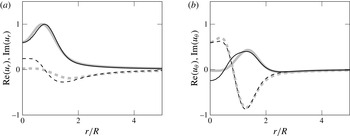
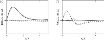
A similar comparison is made in figure 7 between the mode (1,5) and the mode (C,1,2) of the columnar vortex (figure 4). The latter mode has been chosen for the comparison since it has the same frequency as the mode (1,5). The radial velocity profiles of these modes for the pancake and columnar vortices are very similar. For the columnar vortex, the mode (C,1,2) corresponds to a mixed mode between centrifugal instability and Gent–McWilliams instability (also called internal instability). The latter instability comes from a destabilization of the long wavelength bending mode by the critical layer where
 ${\it\Omega}(r_{c})={\it\omega}_{r}$
when the vorticity gradient is positive
 ${\it\zeta}^{\prime }(r_{c})>0$
(Yim & Billant Reference Yim and Billant2015). We can see in figure 7 that the radial and azimuthal velocity components of the perturbation are non-zero on the axis in contrast to the centrifugal mode (1,1) (figure 6). Thus, the perturbation partially bends the vortex. For a columnar vortex in strongly stratified fluids without background rotation, such a bending mode transforms continuously into a centrifugal mode, explaining why there is a single continuous branch in figure 4. However, in the presence of strong background rotation, the centrifugal instability disappears and only the Gent–McWilliams instability remains (Gent & McWilliams Reference Gent and McWilliams1986; Smyth & McWilliams Reference Smyth and Mcwilliams1998; Yim & Billant Reference Yim and Billant2015). For a pancake vortex in a stratified fluid, a continuous transition is also observed: the modes (1,4) (figure 5
c) and (1,6) also exhibit the characteristics of the centrifugal mode but with a non-zero velocity on the axis, as for the mode (1,5). Interestingly, these modes seem to concentrate in the regions where the vertical shear
 $|\partial u_{b{\it\theta}}/\partial z|$
is maximum
 $|z|/{\it\Lambda}=r/R\simeq 0.71$
. The mode (1,7) in figure 4 has a very small growth rate and its frequency is slightly negative. As shown in appendix B, the radial velocity of this mode (figure 5
d) is almost identical to the base angular velocity. It corresponds to the displacement mode which derives from translational invariance and translates the base flow horizontally.
Comparison between the (a) radial
 $u_{r}$
and (b) azimuthal
 $u_{{\it\theta}}$
velocities of the eigenmodes (C,1,1) of columnar (thick grey lines) and (1,1) of pancake vortices (light black lines) in figure 4. ——; real and - - -; imaginary parts.

Same as in figure 6 but for the modes (C,1,2) and (1,5).

Growth rate (
 ${\it\omega}_{i}/{\it\Omega}_{0}$
) and frequency (
 ${\it\omega}_{r}/{\it\Omega}_{0}$
) spectra for a pancake vortex (
 ${\it\alpha}=1.2$
) (○: for symmetric and

 ${\it\alpha}=\infty$
) (

 $m=2$
,
 $F_{h}=0.5$
and
 $Re=10^{4}$
. The modes (C,2,1) and (C,2,1) correspond to modes of the columnar vortex whose frequencies are the same as the modes (2,1) and (2,3), respectively.

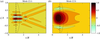
Real part of the radial velocity perturbation Re(
 $u_{r}$
) of (a) mode (2,1) and (b) mode (2.3) of figure 8. The dotted line indicates the contour where the angular velocity of the base vortex is
 ${\it\Omega}=0.1{\it\Omega}_{0}$
. The dashed line represents the contour where the Rayleigh discriminant
 ${\it\Phi}$
vanishes.

3.3
$m=2$

Figure 8 shows an example of the spectrum for
 $m=2$
,
 $F_{h}=0.5$
and
 $Re=10^{4}$
. For a pancake vortex with aspect ratio
 ${\it\alpha}=1.2$
, there are three unstable modes (labelled (2,1)–(2,3)). The radial velocity perturbation of the most unstable mode (2,1) is shown in 9(a). The perturbation is maximum near
 $r/R=1$
and localized within
 $-0.5<z/{\it\Lambda}<0.5$
with a typical wavelength
 ${\it\lambda}\simeq 0.26{\it\Lambda}$
. In the vortex core, it closely resembles the most unstable centrifugal modes for
 $m=0$
(figure 2
a) and
 $m=1$
(figure 5
a). However, inclined rays can also be seen outside the vortex core. We shall see in § 4.2 that these perturbations outside the vortex core correspond to internal gravity waves radiated by the centrifugal mode. For
 $m=1$
, such radiation of internal waves also exists but their amplitude is too weak to be visible in figure 5(a). The mode (2,2) in figure 8 is a centrifugal mode similar to the mode (2,1) but the mode (2,3) is different. As seen in figure 9(b), its radial velocity is localized in the core and does not exhibit many oscillations along the vertical. For a columnar vortex, the spectra possess two separate branches (thick grey lines in figure 8). The branch near
 ${\it\omega}_{r}\simeq 0.45{\it\Omega}_{0}$
corresponds to centrifugal instability while the one near
 ${\it\omega}_{r}=0.27{\it\Omega}_{0}$
corresponds to shear instability. We see that there is a good correspondence with the spectrum of the pancake vortex even if the maximum growth rates for the columnar vortex are again higher than those for the pancake vortex. This confirms that the modes (2,1) and (2,2) are centrifugal modes and shows that the mode (2,3) is due to shear instability. In addition, the radial velocity profiles of the eigenmodes of columnar and pancake vortices are very close both for centrifugal (figure 10) and shear (figure 11) instabilities. Oscillations at large radii corresponding to radiation of gravity waves are also observed for the centrifugal mode of the columnar vortex (figure 10
a).
Comparison between the (a) radial
 $u_{r}$
and (b) azimuthal
 $u_{{\it\theta}}$
velocities of the eigenmodes (C,2,1) of columnar (thick grey lines) and (2,1) of pancake vortices (light black lines) in figure 8. ——; Real and - - -; Imaginary parts.

Same as in figure 10 but for the modes (C,2,2) and (2,3).

4 Parametric study of the most unstable modes
In this section, we investigate the effects of the control parameters
 $({\it\alpha},F_{h},Re,Sc)$
on the most unstable mode of each instability type for
 $m=0,1,2$
. The control parameters are varied only in the range
 $F_{h}/{\it\alpha}\leqslant \exp (3/4)/\sqrt{2}\simeq 1.5$
, ensuring that the total density gradient
 $\partial {\it\rho}_{t}/\partial z=-{\it\rho}_{0}N^{2}/g+\partial {\it\rho}_{b}/\partial z$
is everywhere negative. When
 $F_{h}/{\it\alpha}\geqslant 1.5$
, the maximum density gradient, which is located at
 $r=0$
,
 $z=\pm \sqrt{3}/2$
, is positive so that gravitational instability can occur.
(a) Growth rate and (b) frequency of the most unstable modes of each instability type as a function of
 ${\it\alpha}$
, for
 $F_{h}=0.5$
and
 $Re=10^{4}$
. Centrifugal modes:

 $m=0$
,

 $m=1$
,

 $m=2$
; Shear mode:

 $m=2$
.

Real part of the radial velocity perturbation Re(
 $u_{r}$
) of the most unstable mode for different aspect ratios: centrifugal instability for
 $m=2$
for (a)
 ${\it\alpha}=0.5$
, (b)
 ${\it\alpha}=1$
, (c)
 ${\it\alpha}=2$
and shear instability for
 $m=2$
for (d)
 ${\it\alpha}=1$
, (e)
 ${\it\alpha}=2$
for
 $F_{h}=0.5$
and
 $Re=10^{4}$
. The dotted line indicates the contour where the angular velocity of the base vortex is
 ${\it\Omega}=0.1{\it\Omega}_{0}$
. Note that the vertical scale is not scaled by
 ${\it\Lambda}$
as before but by
 $R$
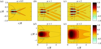
.

4.1 Effect of the aspect ratio
When the aspect ratio is increased from
 ${\it\alpha}=0.35$
to
 ${\it\alpha}=2$
for
 $F_{h}=0.5,Re=10^{4}$
, the growth rate of the most unstable centrifugal modes for
 $m=0,1$
and
 $2$
increase slightly while the corresponding frequencies are almost constant (figure 12). The lower limit
 ${\it\alpha}=0.35$
corresponds to the appearance of gravitational instability. It is interesting to note that the overall most unstable centrifugal mode for these parameters is not the axisymmetric mode but the
 $m=1$
mode. The growth rate of the most unstable shear mode (
 $m=2$
) is positive only for
 ${\it\alpha}\geqslant 1$
and increases with
 ${\it\alpha}$
. The most unstable centrifugal eigenmode and shear eigenmode for
 $m=2$
are displayed in figure 13 for different values of the aspect ratio. The vertical scale is non-dimensionalised by
 $R$
instead of
 ${\it\Lambda}$
in order to have the same reference vertical scale for the three plots. Hence, we can see that the wavelength of the centrifugal instability (figure 13
a–c) is approximately the same for all
 ${\it\alpha}$
, but the number of oscillations along the vertical increases as the vortex becomes taller. Correspondingly, the number of distinct centrifugal modes increases with
 ${\it\alpha}$
since the vertical confinement decreases: for example for
 $m=2$
, for
 ${\it\alpha}=0.5$
there is one unstable mode; for
 ${\it\alpha}=1$
, two modes and for
 ${\it\alpha}=2$
, five modes (not shown). In contrast, the height of the shear mode (figure 13
d,e) is proportional to the aspect ratio.
4.2 Effect of the Froude number
Figure 14 shows that the growth rates of the most unstable centrifugal modes for
 $m=0,1,2$
increase with the Froude number for
 ${\it\alpha}=1,Re=10^{4}$
. The growth rates seem to asymptote to constant values as the Froude number increases but the pancake vortex becomes gravitationally unstable beyond
 $F_{h}=1.5$
for
 ${\it\alpha}=1$
. The centrifugal modes for
 $m=0$
and
 $m=2$
are stabilized when the Froude number goes below
 $F_{h}=0.3{-}0.35$
. In contrast, the centrifugal mode
 $m=1$
continues to be unstable for smaller Froude number. Hence, the mode
 $m=1$
is the most unstable mode when
 $F_{h}\leqslant 0.8$
while the axisymmetric mode is most unstable only above this threshold. The shear mode for
 $m=2$
exists when
 $F_{h}\leqslant 0.5$
and its growth rate increases as the Froude number decreases. As seen in figure 14
b, the frequencies of the modes are almost independent of the Froude number except for
 $m=1$
for low Froude number
 $F_{h}\leqslant 0.5$
. The most unstable eigenmodes for
 $m=1$
and
 $m=2$
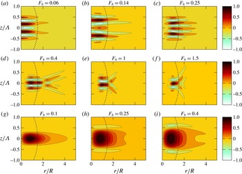
are shown in figure 15 for different Froude numbers. When
 $F_{h}$
decreases, the typical wavelength of the eigenmode for
 $m=1$
(figure 15
a–c) varies little but the location of the maximum moves from
 $r/R\simeq 1$
to the axis
 $r=0$
. Thus, the centrifugal mode transforms continuously into a bending mode (Gent–McWilliams instability) as
 $F_{h}$
decreases. In contrast, centrifugal instability for
 $m=2$
(figure 15
d–f) remains at the same radial location but the angle
 ${\it\theta}$
of the rays with respect to the vertical decreases when the Froude number increases. This angle is in good agreement with the dispersion relation of internal waves
 $\cos {\it\theta}={\it\omega}_{r}/N$
where
 ${\it\omega}_{r}\simeq 0.45$
is the frequency of the centrifugal mode. Therefore, the perturbations outside the vortex core correspond to internal waves forced by centrifugal instability. We can also note in figure 15(d–f) that the typical wavelength of the centrifugal mode for
 $m=2$
increases slightly with the Froude number:
 ${\it\lambda}\simeq 0.28{\it\Lambda}(F_{h}=0.4);{\it\lambda}\simeq 0.34{\it\Lambda}(F_{h}=1)$
and
 ${\it\lambda}\simeq 0.36{\it\Lambda}(F_{h}=1.5)$
. The height of the shear mode (figure 15
g–i) also increases slightly with the Froude number.


Real part of the radial velocity perturbation Re(
 $u_{r}$
) of the most unstable modes for different Froude numbers: for
 $m=1$
for (a)
 $F_{h}=0.06$
, (b)
 $F_{h}=0.14$
and (c)
 $F_{h}=0.25$
, for centrifugal instability for
 $m=2$
for (d)
 $F_{h}=0.4$
, (e)
 $F_{h}=1$
, (f)
 $F_{h}=1.5$
and for shear instability for
 $m=2$
for (g)
 $F_{h}=0.1$
, (h)
 $F_{h}=0.25$
and (i)
 $F_{h}=0.4$
for
 ${\it\alpha}=1$
and
 $Re=10^{4}$
. The dotted lines indicate the contour where the angular velocity of the base vortex is
 ${\it\Omega}=0.1{\it\Omega}_{0}$
.


4.3 Effect of the Reynolds number
Finally, figure 16 shows the dependence of the growth rate and frequency of the most unstable modes on the Reynolds number for a fixed aspect ratio and Froude number:
 ${\it\alpha}=0.5,F_{h}=0.5$
. The general tendency with
 $Re$
is similar to that with the Froude number: the growth rate of the centrifugal modes increases with
 $Re$
for all azimuthal wavenumbers
 $m$
and tends to asymptote to a constant. For
 $Re\leqslant 3\times 10^{4}$
, the centrifugal mode
 $m=1$
is the most unstable mode while it is the axisymmetric mode above. The centrifugal modes for
 $m=0$
and
 $2$
are both stabilized when
 $Re\leqslant 5\times 10^{3}$
whereas
 $m=1$
remains unstable even for small
 $Re$
. The eigenmode for
 $m=1$
then changes gradually to the bending mode. The shear mode for
 $m=2$
is not present at any Reynolds number for the parameters
 ${\it\alpha}=0.5,F_{h}=0.5$
. The reasons why will be explained in § 6. Figure 17 shows the radial velocity of the dominant eigenmode for
 $m=1$
and
 $m=2$
for different
 $Re$
. As observed when
 $F_{h}$
decreases (§ 4.2), the centrifugal mode for
 $m=1$
(figure 17
a–c) changes continuously into a bending mode when
 $Re$
decreases. The typical wavelength increases significantly as
 $Re$
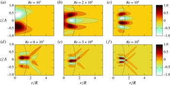
increases. Regarding the centrifugal mode for
 $m=2$
(figure 17
d–f), the typical vertical wavelength clearly decreases with
 $Re$
:
 ${\it\lambda}=0.3{\it\Lambda},0.2{\it\Lambda}$
and
 $0.13{\it\Lambda}$
, for
 $Re=8\times 10^{3},3\times 10^{4}$
and
 $10^{5}$
, respectively.
Real part of the radial velocity perturbation Re(
 $u_{r}$
) of the most unstable mode for different Reynolds numbers for
 $m=1$
for (a)
 $Re=10^{3}$
, (b)
 $Re=2\times 10^{3}$
and (c)
 $Re=10^{4}$
and for
 $m=2$
for (d)
 $Re=8\times 10^{3}$
, (e)
 $Re=3\times 10^{4}$
, (f)
 $Re=10^{5}$
for
 ${\it\alpha}=0.5$
and
 $F_{h}=0.5$
. The dotted lines indicate the contour where the angular velocity of the base vortex is
 ${\it\Omega}=0.1{\it\Omega}_{0}$
.

Growth rate (
 ${\it\omega}_{i}/{\it\Omega}_{0}$
) and frequency (
 ${\it\omega}_{r}/{\it\Omega}_{0}$
) spectra for different Schmidt numbers: (a)
 $Sc=1$
, (b)
 $Sc=7$
and (c)
 $Sc=700$
for a pancake vortex for
 ${\it\alpha}=0.5$
(○: for symmetric and


 $m=0$
,
 $F_{h}=0.5$
and
 $Re=10^{4}$
.

4.4 Effect of the Schmidt number
So far the Schmidt number has been kept to
 $Sc=1$
. Figure 18 shows now the spectra for three different Schmidt numbers
 $Sc=1$
,
 $Sc=7$
and
 $Sc=700$
for
 $m=0$
,
 ${\it\alpha}=0.5,F_{h}=0.5$
and
 $Re=10^{4}$
. The values
 $Sc=7$
and
 $Sc=700$
are typical of temperature and salinity, respectively. When
 $Sc=7$
(figure 18
b), the maximum growth rate is lower and the frequency is no longer zero compared to
 $Sc=1$
(figure 18
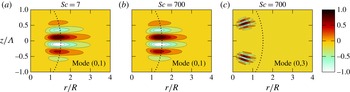
a). A similar spectrum is observed for a columnar vortex for the same parameters (grey line). Nevertheless, the structure of the most unstable eigenmode (0,1) for the pancake vortex (figure 19
a) is similar to the one for
 $Sc=1$
(figure 2). When
 $Sc$
is increased to 700, these centrifugal modes remain approximately at the same location (figure 18
c) and their structure does not change (figure 19
b). However, a new instability branch appears near the origin (figure 18
c). The most unstable eigenmode of this branch (0,3) (figure 19
c) exhibits inclined short-wavelength oscillations localized in the top and bottom of the vortex. Such mode is similar to those observed by Meunier, Miquel & Le Dizès (Reference Meunier, Miquel, Le Dizès, Chowdhury and Alam2014) around a rotating ellipsoid in a stratified fluid. This instability, which is absent in the columnar configuration, is called the McIntyre instability (McIntyre Reference McIntyre1970). It is due to a double-diffusion phenomenon between momentum and mass diffusion. This instability is however less unstable than the centrifugal instability and will not be investigated further here.
Real part of the radial velocity perturbations Re
 $(u_{r})$
of the mode (a) (0,1) for
 $Sc=7$
and (b) (0,1) and (c) (0,3) for
 $Sc=700$
for
 $m=0,F_{h}=0.5$
and
 $Re=10^{4}$
. The dotted lines indicate the contour where the angular velocity of the base vortex is
 ${\it\Omega}=0.1{\it\Omega}_{0}$
.

Growth rate (
 ${\it\omega}_{i}/{\it\Omega}_{0}$
) and frequency (
 ${\it\omega}_{r}/{\it\Omega}_{0}$
) spectra for (a)
 $m=1$
,
 ${\it\alpha}=0.5,F_{h}=1/3,Re=10^{4}$
and (b)
 $m=2$
,
 ${\it\alpha}=1.2,F_{h}=0.5,Re=10^{4}$
for pancake (discrete symbols) and columnar (continuous lines) vortices for different Schmidt numbers: ○,

 $Sc=1$
; ▵,

 $Sc=7$
and ▫,

 $Sc=700$
.

Figure 20 shows the effect of the Schmidt number on the spectra of the azimuthal wavenumbers
 $m=1$
and
 $m=2$
presented in figures 4 and 8, respectively. In contrast to the axisymmetric mode, there is almost no differences between the spectra for
 $Sc=1$
,
 $Sc=7$
and
 $Sc=700$
for these azimuthal wavenumbers.
5 Scaling laws for the growth rate of centrifugal instability
Billant & Gallaire (Reference Billant and Gallaire2005) have derived an asymptotic formula for the growth rate of centrifugal instability for columnar vortices for large vertical wavenumber (
 $k\gg 1$
) in the inviscid limit:
 $$\begin{eqnarray}\displaystyle {\it\omega}={\it\omega}^{(0)}-\frac{{\it\omega}^{(1)}N}{k}+O\left(\frac{1}{k^{2}}\right), & & \displaystyle\end{eqnarray}$$
where
 $$\begin{eqnarray}\displaystyle & \displaystyle {\it\omega}^{(0)}=m{\it\Omega}(r_{0})+\text{i}\sqrt{-{\it\phi}(r_{0})}, & \displaystyle\end{eqnarray}$$
 $$\begin{eqnarray}\displaystyle & \displaystyle {\it\omega}^{(1)}=\frac{(2n+1)\text{i}}{2\sqrt{2}}\sqrt{\frac{{\it\phi}^{\prime \prime }(r_{0})-2m^{2}{\it\Omega}^{\prime }(r_{0})^{2}+2\text{i}m\sqrt{-{\it\phi}(r_{0})}{\it\Omega}^{\prime \prime }(r_{0})}{-{\it\phi}(r_{0})}}\sqrt{1-\frac{{\it\phi}(r_{0})}{N^{2}}}, & \displaystyle\end{eqnarray}$$
 $n$
a non-negative integer,
 ${\it\phi}=2{\it\Omega}{\it\zeta}$
and
 $r_{0}$
is given by
 $$\begin{eqnarray}\displaystyle {\it\phi}^{\prime }(r_{0})=-2\text{i}m{\it\Omega}^{\prime }(r_{0})\sqrt{-{\it\phi}(r_{0})}. & & \displaystyle\end{eqnarray}$$
Here, we show that the formula (5.1) can be used to predict the growth rate of centrifugal instability in pancake vortices. First, since centrifugal instability is most unstable in the limit
 $k\rightarrow \infty$
in inviscid fluids, viscous effects on the perturbation can be easily taken into account at leading order in
 $k$
by adding a damping term of the form
 ${\it\nu}k^{2}$
(Lazar, Stegner & Heifetz Reference Lazar, Stegner and Heifetz2013). Thus, (5.1) becomes at leading order:
 $$\begin{eqnarray}\displaystyle {\it\omega}={\it\omega}^{(0)}-\frac{{\it\omega}^{(1)}N}{k}-\text{i}{\it\nu}k^{2}. & & \displaystyle\end{eqnarray}$$
Using (5.5) and imposing
 $$\begin{eqnarray}\displaystyle \frac{\partial {\it\omega}_{i}}{\partial k}=0, & & \displaystyle\end{eqnarray}$$
we can deduce that the most amplified wavenumber is given by
 $$\begin{eqnarray}\displaystyle k_{max}R=\left(\frac{{\it\omega}_{i}^{(1)}ReR}{2F_{h}}\right)^{1/3}, & & \displaystyle\end{eqnarray}$$
where
 $n$
should be set to zero in (5.3) to have the most unstable mode. Substituting
 $k_{max}$
into (5.5) gives the maximum growth rate,
 $$\begin{eqnarray}\displaystyle ({\it\omega}_{i})_{max}={\it\omega}_{i}^{(0)}-\frac{3{\it\Omega}_{0}}{F_{h}^{2/3}Re^{1/3}}\left({\it\omega}_{i}^{(1)}\frac{R}{2}\right)^{2/3}. & & \displaystyle\end{eqnarray}$$
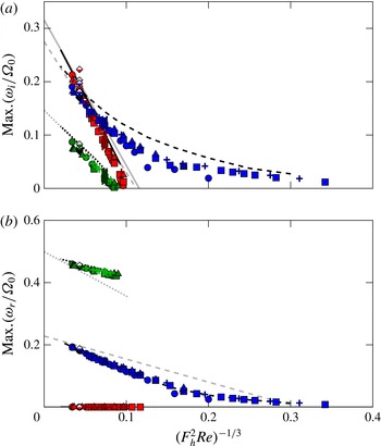
Maximum growth rate (a) and corresponding frequency (b) of centrifugal instability as a function of
 $\mathscr{R}=ReF_{h}^{2}$
for pancake vortices for
 $m=0$
(red symbols),
 $m=1$
(blue symbols) and
 $m=2$
(green symbols) for different control parameters. The grey lines show the theoretical prediction (5.8) and the black lines correspond to numerical results for a columnar vortex for
 $F_{h}=0.5$
and various
 $Re$
for
 $m=0$
(solid lines),
 $m=1$
(dashed lines) and
 $m=2$
(dotted lines). The different symbols correspond to: ● various
 $Re$
for
 ${\it\alpha}=0.5,F_{h}=0.5$
; ▪ various
 $F_{h}$
for
 ${\it\alpha}=0.5,Re=10^{4}$
; ▲ various
 $F_{h}$
for
 ${\it\alpha}=1,Re=10^{4}$
;
 $+$
various
 $F_{h}$
for
 ${\it\alpha}=0.5,Re=3\times 10^{4}$
;
 $\times$
various
 ${\it\alpha}$
for
 $F_{h}=0.5,Re=10^{4}$
; ♦ various
 ${\it\alpha}$
for
 $F_{h}=0.5,Re=5\times 10^{4}$
.

For small Froude number
 $F_{h}$
(i.e. large
 $N$
),
 ${\it\omega}^{(1)}$
becomes independent of
 $F_{h}$
. Hence, (5.8) shows that the maximum growth rate of centrifugal instability is a linear function of
 $(F_{h}^{2}Re)^{-1/3}$
. In other words, the maximum growth rate is only a function of the buoyancy Reynolds number
 $\mathscr{R}=ReF_{h}^{2}$
and is independent of the aspect ratio. The same result applies to the corresponding frequency:
 $$\begin{eqnarray}\displaystyle {\it\omega}_{r}={\it\omega}_{r}^{(0)}-\frac{(2R^{2})^{1/3}{\it\Omega}_{0}{\it\omega}_{r}^{(1)}}{({\it\omega}_{i}^{(1)}\mathscr{R})^{1/3}}. & & \displaystyle\end{eqnarray}$$
The formula (5.8) and (5.9) are shown by dashed lines in figures 14 and 16. They agree well with the numerical results. In addition, figure 21 shows the growth rate and frequency of pancake vortices (symbols) as a function of
 $\mathscr{R}^{-1/3}$
for different Reynolds numbers, Froude numbers and aspect ratios. They all gather on a single curve for each azimuthal wavenumber
 $m=0,1,2$
. The theoretical predictions (5.8) and (5.9) are also plotted with thin grey lines. They agree quite well with the numerical results for pancake vortices for
 $m=0$
and
 $m=2$
. However, the growth rate for
 $m=1$
decreases with
 $\mathscr{R}^{-1/3}$
slower than predicted. The growth rate and frequency computed for a columnar vortex for
 $F_{h}=0.5$
and various
 $Re$
are also shown in figure 21 by black lines. They also agree with the predictions of (5.8) and (5.9) except for
 $m=1$
for which the decrease of the growth rate with
 $\mathscr{R}^{-1/3}$
is also slower than predicted. This slow decrease for large
 $\mathscr{R}^{-1/3}$
is due to the transition between the centrifugal and bending modes at long wavelengths. The formula (5.5) no longer applies in this limit. From figure 21, we can deduce that centrifugal instability for
 $m=0$
and
 $m=2$
is stabilized when
 $\mathscr{R}=ReF_{h}^{2}\lesssim 10^{3}$
while the mode
 $m=1$
becomes stable only when
 $\mathscr{R}\lesssim 16$
. The mode
 $m=1$
is more unstable than
 $m=0$
when
 $\mathscr{R}\lesssim 4.6\times 10^{3}$
.
6 Existence condition of shear instability
In § 4, we have observed that shear instability for
 $m=2$
does not always exist depending on the aspect ratio and Froude number. The purpose of this section is to derive a condition for its existence. To this end, we first consider the stability of a columnar vortex for different
 $F_{h}$
and
 $Re$
. Figure 22(a) shows the growth rate for
 $m=2$
as a function of the rescaled axial wavenumber
 $kRF_{h}$
for different Froude numbers for
 $Re=10^{4}$
. There exist two distinct branches: shear instability for
 $kRF_{h}<1.6$
and centrifugal instability for
 $kRF_{h}\geqslant 5$
. Shear instability is most unstable in the two-dimensional limit (
 $k=0$
) while centrifugal instability is intrinsically three dimensional. Even if the Froude number is varied, the growth rate curves for shear instability remain almost identical when represented as a function of
 $kRF_{h}$
as reported by Deloncle, Chomaz & Billant (Reference Deloncle, Chomaz and Billant2007) for parallel horizontally sheared flows. In contrast, centrifugal instability branch varies greatly with
 $F_{h}$
and becomes more unstable as
 $F_{h}$
increases because its maximum growth rate is a function of
 $F_{h}^{2}Re$
for small
 $F_{h}$
as shown by (5.8). The scaling of the shear branch is consistent with the self-similarity of strongly stratified flows (Billant & Chomaz Reference Billant and Chomaz2001). Such scaling applies as long as the Froude number is small and viscous effects, as measured by the buoyancy Reynolds number
 $\mathscr{R}=ReF_{h}^{2}$
, are negligible. This is the case of all the parameters investigated in figure 22 except
 $F_{h}=0.1$
. The growth rate of shear instability for this Froude number departs slightly from the others because of viscous effects. Similarly, figure 22(b) shows the growth rate for
 $m=2$
for different Reynolds numbers for a fixed Froude number
 $F_{h}=0.5$
. Similar behaviours are observed, the shear instability branch is almost independent of the Reynolds number provided that the buoyancy Reynolds number is not too small. In contrast, the centrifugal instability branch is strongly dependent on
 $Re$
. Because of these different behaviours, shear instability becomes most unstable for small Froude numbers (see the dotted curve for
 $F_{h}=0.35$
and
 $Re=10^{4}$
in figure 22
a) and small Reynolds numbers (see the dotted curve for
 $Re=5\times 10^{3}$
and
 $F_{h}=0.5$
in figure 22
b).
Growth rate for
 $m=2$
for a columnar vortex as a function of the rescaled axial wavenumber
 $kRF_{h}$
(a) for different Froude numbers
 $F_{h}$
at fixed
 $Re=10^{4}$
: - -
 $F_{h}=0.1$
;

 $F_{h}=0.35$
; ——
 $F_{h}=0.5$
;

 $F_{h}=1$
. (b) For different Reynolds numbers
 $Re$
at fixed
 $F_{h}=0.5$
:

 $Re=2\times 10^{3}$
;

 $Re=5\times 10^{3}$
; ——
 $Re=10^{4}$
.

Nevertheless, shear instability is always present in columnar vortices for the range of parameters investigated. In order to explain why it is absent for some parameters for pancake vortices, confinement effects have to be considered. Figure 22 shows that the upper wavenumber cutoff of shear instability is
 $k_{M}R=1.6/F_{h}$
. In other words, the minimum wavelength is
 ${\it\lambda}_{m}\simeq 4F_{h}R$
. Since the typical thickness of the pancake vortex is
 $L_{v}\simeq 2{\it\Lambda}$
, a condition for the existence of shear instability is that at least one wavelength fits along the vertical
 ${\it\lambda}_{m}\leqslant L_{v}$
, i.e.
 $$\begin{eqnarray}\displaystyle \frac{F_{h}}{{\it\alpha}}\leqslant 0.5. & & \displaystyle\end{eqnarray}$$
Figure 23 summarizes the growth rate of the most unstable shear and centrifugal modes for
 $m=2$
as a function of
 $F_{h}/{\it\alpha}$
for various combinations of
 $F_{h}$
,
 $Re$
and
 ${\it\alpha}$
. The growth rates of shear instability collapse approximately into a single curve. The curve for
 ${\it\alpha}=0.5,Re=10^{4}$
(filled diamonds) departs slightly from the others. As explained above, this is because the buoyancy Reynolds number becomes too small as
 $F_{h}$
decreases. If the buoyancy Reynolds number is kept constant
 $\mathscr{R}=2.5\times 10^{3}$
for
 ${\it\alpha}=0.5$
, the growth rate (open diamonds) collapse with the other curves. These curves have the same shape as the growth rate curve of shear instability as a function of
 $kRF_{h}$
for a columnar vortex (figure 22). Furthermore, the growth rate goes to zero for
 $F_{h}/{\it\alpha}=0.5$
in agreement with (6.1). Hence, shear instability is not present in figure 16 because the Froude number
 $F_{h}=0.5$
and aspect ratio
 ${\it\alpha}=0.5$
do not meet the criterion (6.1). In contrast, the growth rate of the most unstable centrifugal mode for
 $m=2$
varies in a disorganized way when represented as a function of
 $F_{h}/{\it\alpha}$
(grey symbols in figure 23). This should be contrasted to figure 21 where a very good collapse for the centrifugal mode was observed when plotted as a function of
 $\mathscr{R}=F_{h}^{2}Re$
.
Finally, figure 24 shows the growth rate for
 $m=2$
as a function of
 $Re$
for
 $F_{h}/{\it\alpha}=0.41$
, i.e. when (6.1) is satisfied. Both centrifugal (dashed line) and shear (solid line) instabilities exist. The growth rate of centrifugal instability strongly depends on
 $Re$
and vanishes when
 $Re\leqslant 5.5\times 10^{3}$
while the growth rate of shear instability is independent of
 $Re$
for
 $Re\geqslant 7\times 10^{3}$
but eventually goes to zero around
 $Re=3\times 10^{3}$
.
Growth rate of the most unstable shear (coloured filled symbols) and centrifugal (grey open symbols) modes as a function of
 $F_{h}/{\it\alpha}$
for different
 $F_{h}$
for fixed
 ${\it\alpha}$
and
 $Re$
:

 ${\it\alpha}=0.5$
,
 $Re=10^{4}$
,

 ${\it\alpha}=0.5$
,
 $Re=3\times 10^{4}$
;

 ${\it\alpha}=1$
,
 $Re=10^{4}$
;

 ${\it\alpha}=1.2$
,
 $Re=10^{4}$
and

 ${\it\alpha}$
for
 $F_{h}=0.5$
and
 $Re=10^{4}$
; ♢ for
 ${\it\alpha}=0.5$
and constant buoyancy Reynolds number
 $\mathscr{R}=ReF_{h}^{2}=2.5\times 10^{3}$
.

Growth rate as a function of
 $Re$
for
 $m=2$
for
 ${\it\alpha}=1.2$
,
 $F_{h}=0.5$
:


7 Instabilities specific to pancake vortices
In the previous sections, we identified and characterized centrifugal and shear instabilities in pancake vortices by comparison to their counterparts in columnar vortices. We restricted the parameter range to
 $F_{h}/{\it\alpha}<1.5$
in order to avoid the occurrence of gravitational instability. In this section, we now focus on the range of parameters close to
 $F_{h}/{\it\alpha}=1.5$
. We shall see that another type of instability can occur in addition to gravitational instability.
Figure 25 shows two examples of spectra for two different Froude numbers such that:
 $F_{h}/{\it\alpha}=1.49$
and
 $F_{h}/{\it\alpha}=1.67$
for otherwise the same parameters:
 ${\it\alpha}=0.5$
,
 $m=2$
and
 $Re=10^{4}$
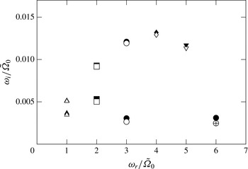
. In figure 25(a), there exist two distinct groups of modes which have different frequencies: the first group (labelled CI) is located around
 ${\it\omega}_{r}/{\it\Omega}_{0}=0.4$
while the second group (labelled BI) is around
 ${\it\omega}_{r}/{\it\Omega}_{0}=0.8$
. The maximum growth rate of these two groups are comparable for these parameters. Two distinct groups are also seen for
 $F_{h}/{\it\alpha}=1.67$
(figure 25
b), i.e. when the parameters are above the threshold for gravitational instability. The frequencies are approximately the same as for
 $F_{h}/{\it\alpha}=1.49$
but the second group near
 ${\it\omega}_{r}/{\it\Omega}=0.8$
(labelled GI) has now a much larger maximum growth rate.
Growth rate (
 ${\it\omega}_{i}/{\it\Omega}_{0}$
) and frequency (
 ${\it\omega}_{r}/{\it\Omega}_{0}$
) spectra for a pancake vortex (○: for symmetric and

 $F_{h}/{\it\alpha}=1.49$
(b)
 $F_{h}/{\it\alpha}=1.67$
for the same parameters
 $m=2,{\it\alpha}=0.5$
and
 $Re=10^{4}$
.

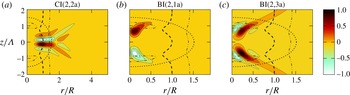
Figure 26 shows the radial velocity perturbation of the CI and BI modes labelled (2,2a), (2,1a) and (2,3a) in figure 25(a). The thick dashed line in figure 26 indicates the contour where the generalized Rayleigh discriminant changes sign. The CI mode (2,2a) is a centrifugal mode with similar characteristics as those described previously. The BI mode (2,1a), however, shows different properties. The mode is concentrated near
 $r/R=0$
and
 $z/{\it\Lambda}=\pm 0.7$
which is near the regions of maximum total density vertical gradient. Yet, the flow is stable to gravitational instability since
 $F_{h}/{\it\alpha}=1.49\leqslant 1.5$
. The second BI mode (2,3a) is located in the same regions but exhibits more radial oscillations and some internal waves rays.
Real part of the radial velocity perturbation Re(
 $u_{r}$
) for
 $F_{h}/{\it\alpha}=1.49,m=2,Re=10^{4},{\it\alpha}=0.5$
of the modes: (a) CI (2,2a) (b) BI (2,1a) (c) BI (2,3a) (see figure 25
a). The thick dashed line represents the contour where the Rayleigh discriminant
 ${\it\Phi}$
vanishes. The dotted line indicates the contour where the angular velocity of the base vortex is
 ${\it\Omega}=0.1{\it\Omega}_{0}$
. The potential vorticity radial gradient along isopycnal changes sign on the double dotted dashed lines.

Real part of the radial velocity perturbation Re(
 $u_{r}$
) for
 $F_{h}/{\it\alpha}=1.67,m=2,Re=10^{4},{\it\alpha}=0.5$
of the modes: (a) GI (2,1b), (b) GI (2,5b) and (c) CI (2,8b) (see figure 25
b). The thick dashed line represents the contour where the Rayleigh discriminant
 ${\it\Phi}$
vanishes. The thick dash dotted line delimits the regions where the vertical gradient of total density
 $\partial {\it\rho}_{t}/\partial z$
is positive. The dotted line indicates the contour where the angular velocity of the base vortex is
 ${\it\Omega}=0.1{\it\Omega}_{0}$
. The potential vorticity radial gradient along isopycnal changes sign on the double dotted dashed lines.

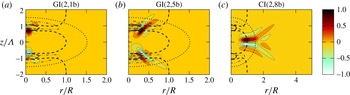
The GI and CI modes (2,1b), (2,5b) and (2,8b) of figure 25(b) are shown in figure 27. The GI mode (2,1b) (figure 27
a) is localized in the regions delimited by thick dashed lines where the vertical gradient of total density
 $\partial {\it\rho}_{t}/\partial z$
is positive. This proves that this mode corresponds to gravitational instability. The GI mode (2,5b) (figure 27
b) shows more complicated structures but is also localized near the regions of positive vertical gradient of total density. The phase velocity of these gravitational modes
 ${\it\omega}_{r}/m\simeq 0.45{\it\Omega}_{0}$
is close to the angular velocity of the base flow
 ${\it\Omega}\simeq 0.47{\it\Omega}_{0}$
at the point (
 $r=0,z=\sqrt{3}/2{\it\Lambda}$
) where the total density vertical gradient is maximum. The CI mode (2,8b) is a centrifugal mode similar to mode (2,2a) shown in 26(a).
Figure 28(a) shows the growth rate of the most unstable BI modes as a function of
 $F_{h}/{\it\alpha}$
for different
 $m$
for two different fixed aspect ratios
 ${\it\alpha}=0.4$
and
 ${\it\alpha}=0.5$
for varying
 $F_{h}$
, and for fixed
 $F_{h}=0.74$
for varying
 ${\it\alpha}$
. As can be seen, the azimuthal wavenumbers
 $m=1,2,3$
are unstable but not
 $m=0$
and
 $m\geqslant 4$
. The growth rate for each
 $m$
is mostly a function of
 $F_{h}/{\it\alpha}$
only. The curve for
 $m=3$
and
 ${\it\alpha}=0.4$
departs however slightly from the two other curves. BI modes only exist in a small range:
 $1.43\leqslant F_{h}/{\it\alpha}\leqslant 1.5$
, i.e. just below the threshold for gravitational instability. This means that BI modes are unstable only when the isopycnals are strongly deformed. Figure 28(b) further shows that the growth rates of the BI modes decrease when the Reynolds number decreases for a fixed aspect ratio and Froude number
 ${\it\alpha}=0.5,F_{h}=0.74$
. When
 $Re\leqslant 3\times 10^{3}$
, BI modes are stable.
Growth rate of the most unstable BI modes as a function of (a)
 $F_{h}/{\it\alpha}$
: for
 ${\it\alpha}=0.4$

 ${\it\alpha}=0.5$

 $F_{h}=0.74$

 $Re=2\times 10^{4}$
and (b) as a function of
 $Re$
for
 ${\it\alpha}=0.5$
and
 $F_{h}=0.74$
for different azimuthal wavenumbers:

 $m=0$
,

 $m=1$
,

 $m=2$
and

 $m=3$
.

Isopycnals of the base vortex for
 ${\it\alpha}=0.5$
for different Froude numbers (a)
 $F_{h}/{\it\alpha}=1.33$
, (b)
 $F_{h}/{\it\alpha}=1.49$
, (c)
 $F_{h}/{\it\alpha}=1.67$
. The vertical gradient of total density
 $\partial {\it\rho}_{t}/\partial z=0$
vanishes on the thick dashed line - - - (red) in (c). The dotted lines

 ${\it\Omega}=0.1{\it\Omega}_{0}$
. The potential vorticity radial gradient along isopycnals changes sign on the double dotted dashed lines.

In order to understand the origin of the BI modes, figure 29(b,c) show the total base density
 ${\it\rho}_{t}$
for the same Froude numbers
 $F_{h}/{\it\alpha}=1.49$
and
 $F_{h}/{\it\alpha}=1.67$
as in figure 25. The density
 ${\it\rho}_{t}$
for a smaller Froude number
 $F_{h}/{\it\alpha}=1.33$
is also displayed for comparison (figure 29
a). When
 $F_{h}/{\it\alpha}$
increases, the isopycnals are more and more deformed in the vortex core due to the thermal wind relation (2.6). This suggests that BI modes could be due to baroclinic instability. A necessary condition for baroclinic instability is that the potential vorticity gradient along isopycnals
 $$\begin{eqnarray}\displaystyle \left.\frac{\partial {\it\Pi}}{\partial r}\right|_{{\it\rho}_{t}}=\frac{\partial {\it\Pi}}{\partial r}\frac{\partial {\it\rho}_{t}}{\partial z}-\frac{\partial {\it\Pi}}{\partial z}\frac{\partial {\it\rho}_{t}}{\partial r}, & & \displaystyle\end{eqnarray}$$
changes sign somewhere in the flow (Eliassen Reference Eliassen1983; Hoskins, McIntyre & Robertson Reference Hoskins, McIntyre and Robertson1985). The potential vorticity reads
 ${\it\Pi}={\bf\omega}_{b}\boldsymbol{\cdot }\boldsymbol{{\rm\nabla}}{\it\rho}_{t}$
where
 ${\bf\omega}_{b}$
is the base vorticity
 ${\bf\omega}_{b}=-\partial (r{\it\Omega})/\partial z\boldsymbol{e}_{r}+1/r\partial (r^{2}{\it\Omega})/\partial r\boldsymbol{e}_{z}$
. The double dotted dashed lines in figure 26 indicate the contours where (7.1) vanishes. The BI modes are located in the vortex core in the vicinity of these lines. This strongly suggests that BI modes are due to baroclinic instability. However, the condition (7.1) is also satisfied for
 $F_{h}/{\it\alpha}=1.33$
(figure 29
a) and continues to be satisfied as
 $F_{h}/{\it\alpha}$
decreases further while BI modes disappear for
 $F_{h}/{\it\alpha}\leqslant 1.43$
for
 ${\it\alpha}=0.5$
and
 $Re=2\times 10^{4}$
(figure 28
a).
To understand this, it is interesting to consider a simple model consisting in a vortex with uniform angular velocity along the radial direction but varying linearly along the vertical direction:
 $$\begin{eqnarray}\displaystyle {\it\Omega}=\tilde{{\it\Omega}}_{0}-\tilde{{\it\Omega}}_{1}z, & & \displaystyle\end{eqnarray}$$
where
 $\tilde{{\it\Omega}}_{0}$
and
 $\tilde{{\it\Omega}}_{1}$
are constants. The corresponding base density is given from the thermal wind relation (2.6) as
 $$\begin{eqnarray}\displaystyle {\it\rho}_{b}=\frac{{\it\rho}_{0}}{g}r^{2}\tilde{{\it\Omega}}_{1}(\tilde{{\it\Omega}}_{0}-\tilde{{\it\Omega}}_{1}z). & & \displaystyle\end{eqnarray}$$
Such angular velocity and density fields are the simplest local approximation of the base flow in the regions where the BI modes develop. For simplicity, we further consider that the base flow (7.2)–(7.3) is bounded in a rigid cylinder of radius
 $R$
and height
 $H$
between
 $z=-H/2$
and
 $z=H/2$
. We also assume that the vertical variations of the angular velocity are weak, i.e.
 $\tilde{{\it\Omega}}_{1}H\ll \tilde{{\it\Omega}}_{0}$
. In appendix A, it is shown that the linearized equations (2.12)–(2.16) in the inviscid limit can be approximated at leading order in
 $\tilde{{\it\Omega}}_{1}$
by a single equation for the pressure
 $$\begin{eqnarray}\displaystyle \frac{1}{r}\frac{\partial }{\partial r}\left(r\frac{\partial p}{\partial r}\right)+\left[-\frac{m^{2}}{r^{2}}+4\tilde{F_{h}}^{2}\frac{\partial ^{2}}{\partial z^{2}}\right]p=0+O(\tilde{{\it\Omega}}_{1}), & & \displaystyle\end{eqnarray}$$
where
 $\tilde{F_{h}}=\tilde{{\it\Omega}}_{0}/N$
. The general solution of (7.4) which is finite at
 $r=0$
is
 $$\begin{eqnarray}\displaystyle p=\text{J}_{m}(2\tilde{F_{h}}kr)[A\cosh kz+B\sinh kz], & & \displaystyle\end{eqnarray}$$
where
 $\text{J}_{m}$
is the Bessel function of order
 $m$
of the first kind and
 $A$
and
 $B$
are constants. By imposing that the vertical velocity vanishes at the top and bottom:
 $u_{z}(z=\pm H/2)=0$
, we obtain the dispersion relation
 $$\begin{eqnarray}\displaystyle {\it\omega}=m\tilde{{\it\Omega}}_{0}+\frac{m\tilde{{\it\Omega}}_{1}}{k}\sqrt{\left(1-\frac{kH}{2\tanh (kH/2)}\right)\left(1-\frac{kH\tanh (kH/2)}{2}\right)}. & & \displaystyle\end{eqnarray}$$
This relation is very similar to the well-known dispersion relation for baroclinic instability of a linear shear flow in a quasi-geostrophic fluid (Eady Reference Eady1949). In order that the normal velocity vanishes at
 $r=R$
, we have also to impose
 $$\begin{eqnarray}\displaystyle 2\tilde{F_{h}}kR={\it\mu}_{m,n}, & & \displaystyle\end{eqnarray}$$
where
 ${\it\mu}_{m,n}$
is the
 $n$
th root of the Bessel function of the first kind of order
 $m$
. As it is well known from the Eady problem (Vallis Reference Vallis2006), (7.6) requires
 $kH\leqslant 2.4$
to have an instability. Combining this condition with (7.7) gives therefore
 $$\begin{eqnarray}\displaystyle \frac{\tilde{F_{h}}}{\tilde{{\it\alpha}}}\geqslant \frac{{\it\mu}_{m,n}}{4.8}, & & \displaystyle\end{eqnarray}$$
where
 $\tilde{{\it\alpha}}=H/R$
is the aspect ratio of the base vortex. Since
 ${\it\mu}_{m,n}\geqslant {\it\mu}_{1,1}=3.83$
, (7.8) gives the condition for instability
 $\tilde{F_{h}}/\tilde{{\it\alpha}}>0.8$
. Below this threshold, the unstable modes predicted by (7.6) are too large to fit inside the cylinder containing the base flow. Although this model is very crude, it explains qualitatively why baroclinic instability for the Gaussian vortex (2.1) develops only when the vertical Froude number
 $F_{h}/{\it\alpha}$
is above a critical value.
Stability diagram for
 ${\it\alpha}=0.5$
as a function of
 $Re$
and
 $F_{h}$
for different azimuthal wavenumber
 $m$
: (a)
 $m=0$
, (b)
 $m=1$
, (c)
 $m=2$
. The symbols indicate: ● centrifugal instability, ▪ shear instability, ▵ baroclinic instability and
 $\times$
stable. The solid lines represent the thresholds for centrifugal instability: ——
 $F_{h}^{2}Re=10^{3}$
for
 $m=0$
;
 $F_{h}^{2}Re=16$
for
 $m=1$
;
 $F_{h}^{2}Re=1.6\times 10^{3}$
for
 $m=2$
. The dashed line - - - in (c) is a fitted curve to numerical results and shows the threshold for shear instability. (d) Schematic diagram of stability for all azimuthal wavenumbers. —— CI threshold for each
 $m$
; - - - shear instability (SI) threshold for
 $m=2$
;


 $m=1$
, due to the bending mode which is unstable in the long-wavelength limit, the CI threshold is also marked with bending mode (BM).

8 Instability map for
$Re<10^{4}$

In this section, we build a map of the domains of existence of the different instabilities in the parameter space (
 $Re,F_{h}$
) summarizing the results derived in the previous sections. We focus on the range of Reynolds numbers
 $Re\leqslant 10^{4}$
and low Froude numbers
 $F_{h}\leqslant 0.5{\it\alpha}$
which pertain to laboratory experiments in the strongly stratified regime. Centrifugal instability has been found to occur when
 $\mathscr{R}=ReF_{h}^{2}\geqslant 10^{3},16$
and
 $1.6\times 10^{3}$
for
 $m=0,1,$
and
 $2$
, respectively. These thresholds are shown by solid lines in figure 30(a–c) for
 $m=0,1,2$
, respectively. A symbol is plotted in these figures for each parameter combination (
 $Re,F_{h}$
) that has been computed numerically for the aspect ratio
 ${\it\alpha}=0.5$
. The different symbols indicate if an instability exists or not and its nature. As seen in figure 30(a,c), the threshold for centrifugal instability in terms of the buoyancy Reynolds number
 $\mathscr{R}$
discriminates well the centrifugally unstable and stable domains for
 $m=0$
and
 $m=2$
. For
 $m=1$
, the threshold
 $\mathscr{R}=16$
departs slightly from the observed limit between the stable and unstable regions for moderate Reynolds numbers. This threshold, which has been derived from results for
 $Re\geqslant 10^{4}$
(see figure 21), is therefore less accurate for moderate
 $Re$
. For
 $m=2$
, shear instability develops when
 $F_{h}\leqslant 0.5{\it\alpha}$
for large
 $Re$
(dashed line in figure 30
c). For low
 $Re$
, this threshold becomes dependent of the Reynolds number and the dashed line corresponds to an empirical fit to the observations. Finally, when
 $F_{h}>1.5{\it\alpha}$
(dotted lines), gravitational instability can develop for any azimuthal wavenumber. For Froude numbers just below this threshold, baroclinic instability can also occur for
 $m\geqslant 1$
for sufficiently large Reynolds number.
All these thresholds are plotted together in a single diagram in figure 30(d) for the aspect ratio
 ${\it\alpha}=0.5$
. Only low Reynolds numbers are stable. The maximum Reynolds number
 $Re_{M}$
which is stable is given by the crossing of the thresholds for shear instability and the
 $m=1$
centrifugal instability, i.e. approximately
 $0.5{\it\alpha}\simeq 4/\sqrt{Re_{M}}$
giving
 $Re_{M}\simeq 64/{\it\alpha}^{2}$
. Hence, the size of the stable domain depends strongly on the aspect ratio. For example, the critical Reynolds number
 $Re_{M}$
varies from
 $O(10^{2})$
to
 $O(10^{6})$
for vortices in laboratory experiments for which
 ${\it\alpha}=O(1)$
to oceanic submesoscale vortices (for which background rotation effects are not too important) with
 ${\it\alpha}=O(0.01)$
. Nevertheless, the typical Reynolds number of the latter vortices is higher than
 $Re_{M}$
.
9 Comparison to previous works
It is now possible to attempt some comparisons between the present results and the laboratory experiments of Flór & van Heijst (Reference Flór and van Heijst1996) and the numerical simulations of Beckers et al. (Reference Beckers, Clercx, van Heijst and Verzicco2003).
Flór & van Heijst (Reference Flór and van Heijst1996) have observed unstable monopolar vortices that evolved into multipolar vortices when
 $F=V_{max}/NR_{max}>0.1$
, where
 $V_{max}$
and
 $R_{max}$
are the maximum azimuthal velocity and corresponding radius. In the case of the profile (2.1), we have
 $F_{h}=1.7F$
. Since the aspect ratio of their vortices is around unity
 ${\it\alpha}\sim 1$
, the condition
 $F\geqslant 1$
corresponds to
 $F_{h}/{\it\alpha}\geqslant 0.17$
. At first sight, this seems incompatible with the condition derived herein for the existence of shear instability
 $F_{h}/{\it\alpha}\leqslant 0.5$
. However, the laboratory experiments of Flór & van Heijst (Reference Flór and van Heijst1996) are for low Reynolds numbers
 $O(100)$
so that the lower left part of the stability diagram for
 $m=2$
(figure 30
c) should be considered. Furthermore, the Reynolds number varies together with the Froude number since it is the maximum velocity which is varied. Hence, we travel along a straight oblique line starting from the origin in figure 30(c). If the slope of this line is not too high, it is therefore possible to enter the unstable domain as the Froude number increases. This would mean that the stabilization observed by Flór & van Heijst (Reference Flór and van Heijst1996) for
 $F<0.1$
is mostly due to viscous effects.
Beckers et al. (Reference Beckers, Clercx, van Heijst and Verzicco2003) have also performed experiments and numerical simulations on pancake vortices with an aspect ratio
 ${\it\alpha}\sim 0.4$
. In their numerical simulations, they have not observed any instability for the profile (2.1) in the Reynolds number range
 $[500,10\,000]$
and Froude number range
 $[0.1,0.8]$
. Their definitions of the Reynolds and Froude numbers are related to our definitions by:
 $\tilde{Re}=VR/{\it\nu}=2{\it\alpha}\sqrt{{\rm\pi}}Re$
and
 $\tilde{F}=V/RN=2{\it\alpha}\sqrt{{\rm\pi}}F_{h}$
since they have taken as the velocity scale
 $V=2\sqrt{{\rm\pi}}{\it\Lambda}{\it\Omega}_{0}$
. Hence, using our definitions of
 $Re$
and
 $F_{h}$
, these ranges correspond to
 $340<Re<6700$
and
 $0.2<F_{h}/{\it\alpha}<1.3$
. Therefore, according to our results, they should have observed shear instability when
 $F_{h}/{\it\alpha}<0.5$
and
 $Re$
is sufficiently large. However, Beckers et al. (Reference Beckers, Clercx, van Heijst and Verzicco2003) have obtained their results from perturbed nonlinear simulations. Thus, the base vortex decays by viscous effects during the simulations. For
 ${\it\alpha}<1$
, these effects are mostly due to vertical shear and thus scale like
 ${\it\Omega}_{0}/({\it\alpha}^{2}Re)$
. Since the growth rate of shear instability is at most
 ${\it\omega}_{i}\simeq 0.015{\it\Omega}_{0}$
for
 $F_{h}/{\it\alpha}\geqslant 0.2$
, the ratio between the growth rate and the viscous damping of the base state is only of order ten for
 $Re=6700$
and
 ${\it\alpha}=0.4$
. This ratio is probably not sufficiently high for the perturbations to have time to grow significantly before the base flow has decayed. Higher Reynolds number or lower vertical Froude number would be necessary to observe the shear instability for
 $q=2$
. In contrast, for steeper angular velocity profiles with
 $q\geqslant 3$
, the growth rate of shear instability is higher and Beckers et al. (Reference Beckers, Clercx, van Heijst and Verzicco2003) observed it when the Reynolds number is sufficiently large in the range
 $Re<6700$
. Furthermore, they reported that the growth rate of shear instability decreases when the Froude number increases, which is consistent with our results.
10 Conclusions
In this paper, we have investigated the stability of an axisymmetric pancake vortex with Gaussian angular velocity in both radial and vertical directions in a stratified fluid. The instabilities of columnar vortices such as the centrifugal and shear instabilities have been observed in spite of this pancake shape. The maximum growth rate of centrifugal instability is almost independent of the aspect ratio
 ${\it\alpha}$
, meaning that it is weakly affected by the pancake shape. The asymptotic formula for the growth rate of centrifugal instability at short wavelength derived by Billant & Gallaire (Reference Billant and Gallaire2005) for inviscid columnar vortices has been extended to viscous fluids and applied to pancake vortices. It shows that the maximum growth rate for each azimuthal wavenumber
 $m=0,1,2$
depends only on the buoyancy Reynolds number
 $\mathscr{R}=ReF_{h}^{2}$
, in good agreement with the numerical results for pancake vortices. The critical Froude number for the apparition of centrifugal instability is therefore of the form
 $F_{h}=c/\sqrt{Re}$
, where the constant
 $c$
depends on
 $m$
. We have also found that the azimuthal wavenumber
 $m=1$
is more unstable than the axisymmetric mode for moderate buoyancy Reynolds numbers
 $\mathscr{R}\lesssim 4600$
. In contrast, the shear instability occurring for
 $m=2$
is strongly affected by the pancake shape and observed only when
 $F_{h}\leqslant 0.5{\it\alpha}$
for sufficiently large Reynolds number. This condition can be understood by considering again the columnar configuration: it ensures that the vortex is taller than the minimum wavelength
 ${\it\lambda}_{m}\simeq 4F_{h}R$
of shear instability for a columnar vortex for the same parameters. For
 $m=1$
, a displacement mode exists with almost zero frequency and growth rate.
Two other instabilities specific to the pancake shape have been found. They are due to the deformations of the isopycnals of the base flow. Gravitational instability can occur when the isopycnals overturn, i.e. when
 $F_{h}\geqslant 1.5{\it\alpha}$
. For Froude numbers just below this threshold
 $F_{h}\geqslant 1.43{\it\alpha}$
, baroclinic instability has also been observed. In order to explain this threshold, we have considered a simple model consisting in a sheared vortex with an angular velocity uniform in the radial direction but varying linearly and weakly along the vertical. When the vortex is assumed to be bounded in a cylinder of radius
 $R$
and height
 $H$
, baroclinic instability occurs only when the vertical Froude number is above a threshold. Although this model is only qualitative, it highlights the fact that baroclinic instability cannot always occur because of confinement effects, even if the necessary condition of sign reversal of the potential vorticity gradient is satisfied. In the future, it would be interesting to study the nonlinear dynamics of these instabilities.
Acknowledgements
We are very grateful to X. Garnaud for providing his numerical code and to D. Guy and V. D. Chi Toaï for their technical assistances. We thank also C. Ménesguen and the referees for their helpful comments and suggestions. This work was supported by the National Research Agency (ANR 2011 Blanc SIMI 5-6 012-02).
Appendix A. Stability equations for a vortex with almost uniform angular velocity
In this section, we derive the simplified stability equation (7.4) for a base vortex with angular velocity (7.2), i.e. uniform in the radial direction and varying linearly along the vertical. The associated density field is given by (7.3). In the inviscid limit, (2.12) and (2.13) yield the radial and azimuthal velocities
 $$\begin{eqnarray}\displaystyle & \displaystyle u_{r}=\frac{\text{i}s\partial p/\partial r+2{\it\Omega}\text{i}mp/r+2ru_{z}{\it\Omega}\partial {\it\Omega}/\partial z}{s^{2}-4{\it\Omega}^{2}}, & \displaystyle\end{eqnarray}$$
 $$\begin{eqnarray}\displaystyle & \displaystyle u_{{\it\theta}}=\frac{-2{\it\Omega}\partial p/\partial r-smp/r+\text{i}ru_{z}s\partial {\it\Omega}/\partial z}{s^{2}-4{\it\Omega}^{2}}, & \displaystyle\end{eqnarray}$$
 $s=m{\it\Omega}-{\it\omega}$
. The vertical velocity is obtained from the vertical momentum and density equations (2.14) and (2.15)
 $$\begin{eqnarray}\displaystyle u_{z}=\frac{g/{\it\rho}_{0}\partial {\it\rho}_{b}/\partial ru_{r}-\text{i}s\partial p/\partial z}{N^{2}-s^{2}-g/{\it\rho}_{0}\partial {\it\rho}_{b}/\partial z}. & & \displaystyle\end{eqnarray}$$
Combining (A 1) and (A 3) gives
 $$\begin{eqnarray}\displaystyle u_{z}=\frac{g/{\it\rho}_{0}\partial {\it\rho}_{b}/\partial r(\text{i}s\partial p/\partial r+2{\it\Omega}\text{i}mp/r)/(s^{2}-4{\it\Omega}^{2})-\text{i}s\partial p/\partial r}{N^{2}-s^{2}-g/{\it\rho}_{0}\partial {\it\rho}_{b}/\partial z-g/{\it\rho}_{0}\partial {\it\rho}_{b}/\partial r(2r{\it\Omega}\partial {\it\Omega}/\partial z)/(s^{2}-4{\it\Omega}^{2})}. & & \displaystyle\end{eqnarray}$$
We now assume
 $\tilde{{\it\Omega}}_{1}H\ll \tilde{{\it\Omega}}_{0}$
and
 ${\it\omega}=m\tilde{{\it\Omega}}_{0}+{\it\omega}_{1}$
with
 ${\it\omega}_{1}=O(\tilde{{\it\Omega}}_{1}H)$
. This implies
 $$\begin{eqnarray}\displaystyle s=-{\it\omega}_{1}-m\tilde{{\it\Omega}}_{1}z=O(\tilde{{\it\Omega}}_{1}H). & & \displaystyle\end{eqnarray}$$
Hence, the velocity perturbations can be simplified at leading order in
 $\tilde{{\it\Omega}}_{1}$
to:
 $$\begin{eqnarray}\displaystyle & \displaystyle u_{r}=\frac{\text{i}s\partial p/\partial r+2\text{i}m(\tilde{{\it\Omega}}_{0}-\tilde{{\it\Omega}}_{1}z)p/r}{-4\tilde{{\it\Omega}}_{0}^{2}+8\tilde{{\it\Omega}}_{0}\tilde{{\it\Omega}}_{1}z}+O(\tilde{{\it\Omega}}_{1}^{2}), & \displaystyle\end{eqnarray}$$
 $$\begin{eqnarray}\displaystyle & \displaystyle u_{{\it\theta}}=\frac{-2(\tilde{{\it\Omega}}_{0}-\tilde{{\it\Omega}}_{1}z)\partial p/\partial r-smp/r}{-4\tilde{{\it\Omega}}_{0}^{2}+8\tilde{{\it\Omega}}_{0}\tilde{{\it\Omega}}_{1}z}+O(\tilde{{\it\Omega}}_{1}^{2}), & \displaystyle\end{eqnarray}$$
 $$\begin{eqnarray}\displaystyle & \displaystyle u_{z}=\frac{-\text{i}\tilde{{\it\Omega}}_{1}mp-\text{i}s\partial p/\partial r}{N^{2}}+O(\tilde{{\it\Omega}}_{1}^{2}). & \displaystyle\end{eqnarray}$$
 $$\begin{eqnarray}\displaystyle \text{i}s\left[\frac{1}{r}\frac{\partial }{\partial r}\left(r\frac{\partial p}{\partial r}\right)-\frac{m^{2}}{r^{2}}p+\frac{4\tilde{{\it\Omega}}_{0}^{2}}{N^{2}}\frac{\partial ^{2}p}{\partial z^{2}}\right]=0+O(\tilde{{\it\Omega}}_{1}^{2}). & & \displaystyle\end{eqnarray}$$
Since
 $s$
is different from zero, (A 9) reduces to (7.4). The general solution is given by (7.5). The boundary conditions at
 $r=R$
and
 $z=\pm H/2$
are assumed to be
 $$\begin{eqnarray}\displaystyle & \displaystyle u_{r}(r=R)=0, & \displaystyle\end{eqnarray}$$
 $$\begin{eqnarray}\displaystyle & \displaystyle u_{z}\left(z=\pm \frac{H}{2}\right)=0. & \displaystyle\end{eqnarray}$$
 $\tilde{{\it\Omega}}_{1}$
if
 $$\begin{eqnarray}\displaystyle & \displaystyle p=0\quad \text{at }r=R, & \displaystyle\end{eqnarray}$$
 $$\begin{eqnarray}\displaystyle & \displaystyle s\frac{\partial p}{\partial z}+m\tilde{{\it\Omega}}_{1}p=0\quad \text{at }z=\pm \frac{H}{2}. & \displaystyle\end{eqnarray}$$
 $$\begin{eqnarray}\displaystyle & & \displaystyle \tilde{{\it\Omega}}_{1}m\left[\begin{array}{@{}cc@{}}\displaystyle -\text{sinh}\frac{kH}{2}-\left(\frac{{\it\omega}_{1}}{\tilde{{\it\Omega}}_{1}m}-\frac{H}{2}\right)k\cosh \frac{kH}{2} & \displaystyle \cosh \frac{kH}{2}+\left(\frac{{\it\omega}_{1}}{\tilde{{\it\Omega}}_{1}m}-\frac{H}{2}\right)k\sinh \frac{kH}{2}\\ \displaystyle \sinh \frac{kH}{2}-\left(\frac{{\it\omega}_{1}}{\tilde{{\it\Omega}}_{1}m}+\frac{H}{2}\right)k\cosh \frac{kH}{2} & \displaystyle \cosh \frac{kH}{2}-\left(\frac{{\it\omega}_{1}}{\tilde{{\it\Omega}}_{1}m}+1\frac{H}{2}\right)k\sinh \frac{kH}{2}\end{array}\right]\hspace{-4.0pt}\nonumber\\ \displaystyle & & \displaystyle \quad \times \,\left[\begin{array}{@{}c@{}}A\\ B\end{array}\right]=0.\end{eqnarray}$$
This leads to the dispersion relation
 $$\begin{eqnarray}\displaystyle {\it\omega}_{1}=\frac{m\tilde{{\it\Omega}}_{1}}{k}\sqrt{\left(1-\frac{kH}{2\tanh (kH/2)}\right)\left(1-\frac{kH\tanh (kH/2)}{2}\right)}, & & \displaystyle\end{eqnarray}$$
so that
 ${\it\omega}=m\tilde{{\it\Omega}}_{0}+{\it\omega}_{1}$
is given by (7.6). The stability of the base flow (7.2)–(7.3) has also been directly computed numerically for
 $\tilde{{\it\Omega}}_{0}=1,\tilde{{\it\Omega}}_{1}=0.01,R=5,H=2,N=1.2$
for a large Reynolds number
 $Re=10^{4}$
. Figure 31 shows that the predictions of (7.6) and the numerical results are in good agreement. For
 $m=1,2$
and
 $3$
, there are two unstable modes for each
 $m$
: the primary mode
 $2\tilde{F_{h}}Rk={\it\mu}_{m,1}$
and the secondary mode
 $2\tilde{F_{h}}Rk={\it\mu}_{m,2}$
. For
 $m\geqslant 4$
, only the primary mode is unstable.
Growth rate (
 ${\it\omega}_{i}/\tilde{{\it\Omega}}_{0}$
) and frequency (
 ${\it\omega}_{r}/\tilde{{\it\Omega}}_{0}$
) spectra of the base flow (7.2)–(7.3) for different azimuthal wavenumbers: ▵
 $m=1$
; ▫
 $m=2$
; ○
 $m=3$
; ♢
 $m=4$
; ▿
 $m=5$
;
 $\oplus$
 $m=6$
. Filled symbols indicate the prediction of (A 15) and open symbols show the numerical results for
 $\tilde{{\it\Omega}}_{0}=1$
,
 $\tilde{{\it\Omega}}_{1}=0.01$
,
 $R=5$
,
 $H=2$
, and
 $N=1.2$
for
 $Re=10^{4}$
.

Appendix B. The
$m=1$
displacement mode

For
 $m=1$
, there exists a mode which derives from the translational invariance. This invariance states that the streamfunction
 ${\it\psi}(x,y)$
for the base flow (2.1) translated by arbitrary displacements (
 ${\rm\Delta}x,{\rm\Delta}y$
), i.e.
 ${\it\psi}(x-{\rm\Delta}x,y-{\rm\Delta}y)$
, remains a solution of the two-dimensional Euler equations. The linear perturbation
 ${\it\psi}^{\prime }$
corresponding to a small displacement
 ${\rm\Delta}x,{\rm\Delta}y\ll 1$
is
 $$\begin{eqnarray}\displaystyle {\it\psi}^{\prime }={\it\psi}(x-{\rm\Delta}x,y-{\rm\Delta}y)-{\it\psi}(x,y)=-{\rm\Delta}x\frac{\partial {\it\psi}}{\partial x}-{\rm\Delta}y\frac{\partial {\it\psi}}{\partial y}. & & \displaystyle\end{eqnarray}$$
The radial and azimuthal velocity perturbations are therefore
 $$\begin{eqnarray}\displaystyle & \displaystyle {u_{r}}^{\prime }=-\frac{1}{r}\frac{\partial {\it\psi}^{\prime }}{\partial {\it\theta}}=\frac{u_{b{\it\theta}}}{r}\left[\left(\frac{{\rm\Delta}x}{2\text{i}}-\frac{{\rm\Delta}y}{2}\right)\text{e}^{\text{i}{\it\theta}}-\left(\frac{{\rm\Delta}x}{2\text{i}}+\frac{{\rm\Delta}y}{2}\right)\text{e}^{-\text{i}{\it\theta}}\right], & \displaystyle\end{eqnarray}$$
 $$\begin{eqnarray}\displaystyle & \displaystyle {u_{{\it\theta}}}^{\prime }=\frac{\partial \hat{{\it\psi}^{\prime }}}{\partial r}=\text{i}\frac{\partial u_{b{\it\theta}}}{\partial r}\left[\left(\frac{{\rm\Delta}x}{2\text{i}}-\frac{{\rm\Delta}y}{2}\right)\text{e}^{\text{i}{\it\theta}}+\left(\frac{{\rm\Delta}x}{2\text{i}}+\frac{{\rm\Delta}y}{2}\right)\text{e}^{-\text{i}{\it\theta}}\right], & \displaystyle\end{eqnarray}$$
(a) Theoretical radial velocity of the displacement mode (
 ${\it\Omega}$
) and (b) real part of the radial velocity perturbation Re(
 $u_{r}$
) of the displacement mode for
 $m=1,{\it\alpha}=0.5,F_{h}=0.5$
and
 $Re=10^{4}$
. The dotted line indicates the contour where the angular velocity of the base vortex is
 ${\it\Omega}=0.1{\it\Omega}_{0}$
.

since
 $u_{b{\it\theta}}=\partial {\it\psi}/\partial r$
. Such a perturbation with
 $u_{z}=0,{\it\rho}=0$
is therefore a neutral solution of the linearized equations (2.12)–(2.16) in the inviscid limit. The radial and azimuthal velocities of the eigenmode are therefore
 $(u_{r},u_{{\it\theta}})\propto ({\it\Omega},\text{i}\partial (r{\it\Omega})/\partial r)$
. Figure 32 shows
 ${\it\Omega}$
and the radial velocity perturbation of the displacement mode Re
 $(u_{r})$
computed for
 ${\it\alpha}=0.5,F_{h}=0.5,Ro=\infty$
and
 $Re=10^{4}$
. As can be seen, they are almost identical. The imaginary part of the azimuthal velocity Im(
 $u_{{\it\theta}}$
) is also similar to
 $\partial (r{\it\Omega})/\partial r$
(not shown).