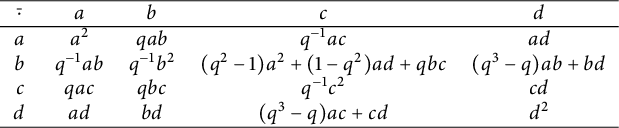
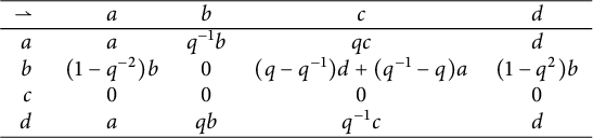
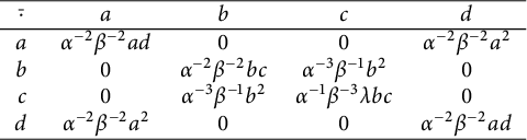
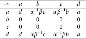
1 Introduction
The notion of braiding is ubiquitous in Mathematics, encompassing low-dimension topology, group theory, category theory, and the theory of the Yang–Baxter equation (YBE). In particular, notions of braided categories [Reference Joyal and Street20], braided groups [Reference Lu, Yan and Zhu24, Reference Majid26, Reference Majid29], and (co)quasitriangular Hopf algebras [Reference Doi10, Reference Drinfeld11, Reference Larson and Towber23, Reference Majid27, Reference Schauenburg36] have been defined around the 1990s, and extensively used ever since.
On the other hand, set-theoretic solutions to the YBE have been studied on suggestion of Drinfeld [Reference Drinfeld12], growing into a vibrant field of research. It is known that braided groups provide solutions to the set-theoretic YBE, and solutions to the YBE are associated with a structure group [Reference Etingof, Schedler and Soloviev13] which turns out to be a braided group. Lu, Yan, and Zhu [Reference Lu, Yan and Zhu24] clarified that a braided group is essentially the same as a matched pair of actions. This is equivalent to bijective 1-cocycles. Afterwards, Guarnieri and Vendramin [Reference Guarnieri and Vendramin18] proved that this is in turn equivalent to a skew brace structure: a notion that has become of capital importance, in its several generalizations (a non-exhaustive list of them being provided by [Reference Brzeziński7, Reference Martin-Lyons and Truman31, Reference Matsumoto33]). Skew braces generalize Rump’s braces [Reference Rump35], and the interplay between skew braces and Yang–Baxter maps generalizes the correspondence between braces and involutive Yang–Baxter maps [Reference Gateva-Ivanova16].
A skew brace is the datum of two group structures
$(G,\cdot )$
 and
$(G,\bullet )$
 on the same set G, satisfying a compatibility. An immediate Hopf-theoretic generalization is the notion of Hopf brace, which is the datum of two Hopf algebra structures
$(H,\cdot ,1,\Delta , \epsilon , S)$
 and
$(H,\bullet , 1,\Delta , \epsilon , T)$
 on the same coalgebra
$(H,\Delta , \epsilon )$
 , satisfying an analogous compatibility [Reference Angiono, Galindo and Vendramin5]. The correspondence between skew braces, matched pairs of actions, and bijective 1-cocycles generalizes naturally to cocommutative Hopf braces, cocommutative matched pairs on a Hopf algebra, and bijective 1-cocycles of cocommutative Hopf algebras. The correspondence between Hopf braces and bijective 1-cocycles is true without the assumption of cocommutativity—in fact, the two structures are strongly related, and the same equivalence holds true in any braided monoidal category [Reference Fernández Vilaboa, González Rodríguez, Ramos Pérez and Rodríguez Raposo15]. However, the assumption of cocommutativity is necessary for the equivalence with matched pairs; which is, in turn, crucial in order to bridge Hopf braces with the world of braiding operators. Thus, cocommutativity seemed hard to relax, without sacrificing the backbone of the correspondence theorem: this is the premise to our investigation.
In this article, we get rid of the cocommutativity hypothesis. As in [Reference Angiono, Galindo and Vendramin5], we consider matched pairs of Hopf algebras, satisfying a braided-commutativity condition: we call them matched pairs of actions on a Hopf algebra (the name being reminiscent of matched pairs of actions on a group, extensively used by Lu, Yan, and Zhu [Reference Lu, Yan and Zhu24] with the name compatible actions). Then, in Section 3, we establish a correspondence between such matched pairs of actions, and Yetter–Drinfeld braces. A Yetter–Drinfeld brace is the datum of a Hopf algebra
$H^\bullet = (H,\bullet , 1, \Delta , \epsilon , T)$
 , and a Hopf algebra
$(H,\cdot ,1, \Delta ,\epsilon ,S)$
 in
$^{H^\bullet }_{H^\bullet }\mathcal {YD}$
 (which we call the transmutation of
$H^\bullet $
 ); where the two structures satisfy some technical hypotheses, and the same compatibility as Hopf braces. It comes out that the notions of Yetter–Drinfeld brace and of Hopf brace coincide in the cocommutative case.
It is natural to ask whether Yetter–Drinfeld braces can be interpreted as 1-cocycles as well. This is positively answered in Section 4.
In Section 5, we present a vast class of Yetter–Drinfeld braces that are, generally, not Hopf braces. Given any coquasitriangular Hopf algebra
$(H,\bullet ,1,\Delta ,\epsilon , T,\mathcal {R})$
 , we shall be able to construct a second operation
$\cdot $
 and a linear map
$S\colon H\to H$
 , yielding a Yetter–Drinfeld brace. In this case, the additional structure on H coincides with the transmutation of
$H^\bullet $
 , introduced by Majid [Reference Majid27, Reference Majid28]. Therefore, we obtain in particular an interpretation of the theory of transmutation, within the frame of Yetter–Drinfeld braces. The map
$\sigma \colon H\otimes H\to H\otimes H$
 ,
$\sigma (a\otimes b):= \mathcal {R}^{-1}(a_1\otimes b_1)b_2\otimes a_2\mathcal {R}(a_3\otimes b_3)$
 is a braiding operator on H. When
$(H^\bullet , \mathcal {R})$
 is cotriangular, the braiding operator
$\sigma $
 is involutive, and the corresponding algebra
$(H,\cdot ,1, \Delta , \epsilon , S)$
 in
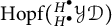
$\mathrm {Hopf}({}^{H^\bullet }_{H^\bullet }\mathcal {YD})$
 is braided-commutative with respect to the braiding of
$^{H^\bullet }_{H^\bullet }\mathcal {YD}$
 .
This entire class of Yetter–Drinfeld braces descending from coquasitriangular Hopf algebras is, in some way, “orthogonal” to the class of cocommutative Hopf braces. When
$(H^\bullet ,\mathcal {R})$
 is a cocommutative coquasitriangular Hopf algebra, the corresponding Yetter–Drinfeld brace is indeed the trivial Hopf brace
$(H,\bullet ,\bullet )$
 .
In conclusion to this article, Section 6 presents several examples of coquasitriangular Hopf algebras, and describes their associated Yetter–Drinfeld braces.
Notations and conventions. We shall denote by  a braided monoidal category, with monoidal product
$\otimes $
 , unit object
 , and braiding
$\sigma $
 . Comforted by the MacLane Coherence theorem, we shall consistently be sloppy on associativity and unit constraints. In the rest of this article, we adopt the notation
$fg$
 for the composition of maps
$f\circ g$
 . The categories of algebras, coalgebras, bialgebras, and Hopf algebras in
$\mathcal {M}$
 will be denoted by
$\mathrm {Mon}(\mathcal {M})$
 ,
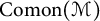
$\mathrm {Comon}(\mathcal {M})$
 ,
$\mathrm {Bimon}(\mathcal {M})$
 , and
$\mathrm {Hopf}(\mathcal {M})$
 , respectively. We shall usually denote by H a bialgebra in
$\mathcal {M}$
 , by
${}_H\!\mathcal {M}$
 ,
$\mathcal {M}_H$
 ,
${}^H\!\mathcal {M}$
 ,
$\mathcal {M}^H$
 ,
${}_H\!\mathcal {M}_H$
 , and
${}^H\!\mathcal {M}^H$
 its category of left and right modules, left and right comodules, bimodules, and bicomodules, respectively. Unless otherwise specified, our setting will be the category
 of vector spaces over
 , with braiding given by the canonical flip
$\tau $
 .
Symbols such as
$\bullet ,\cdot $
 will usually signify the multiplication of an algebra A. Equivalently, the multiplication will be denoted by a map m,
$m_\cdot $
 or
$m_\bullet \colon A\otimes A\to A$
 . The unit is denoted by
$1$
 or, equivalently, by a map
 . The comultiplication and the counit of a coalgebra will be denotedy by
$\Delta $
 and
$\epsilon $
 , respectively. Subscripts will be added for clarity, whenever needed.
In our computations with coalgebras, we shall consistently employ Sweedler’s notation
$\Delta (a)=\sum _{i}a_1^i\otimes a_2^i = a_1\otimes a_2$
 , omitting the summation. A similar notation is adopted for left coactions
$a\mapsto a_{-1}\otimes a_0$
 , and for right coactions
$a\mapsto a_0\otimes a_1$
 .
2 Preliminaries
In this section, we introduce the main notions that we are going to use throughout the article. Namely, we describe matched pairs of actions on a bialgebra, and we survey the fundamentals on Hopf braces.
2.1 Matched pairs of actions
Matched pairs of groups, enabling to define a Zappa–Szép product, have been known for a long time. On the other hand, the notion of a matched pair of Hopf algebras was introduced by Singer [Reference Singer37] in the graded case, and the current notion was introduced by Majid [Reference Majid25]. We consider matched pairs of actions on Hopf algebras, which will turn out to be a subclass of matched pairs of Hopf algebras [Reference Majid30, Definition 7.2.1]. Matched pairs of actions on groups have been already used, e.g., in the seminal work of Lu, Yan, and Zhu [Reference Lu, Yan and Zhu24], and then mutuated in several different contexts, such as for groupoids by Andruskiewitsch [Reference Andruskiewitsch3].
Definition 2.1 Let H be a bialgebra,
$\bullet $
 be its algebra product. A matched pair of actions
$(H,\rightharpoonup ,\leftharpoonup )$
 on H is the datum of a left action
$\rightharpoonup $
 and a right action
$\leftharpoonup $
 of H on itself, such that H is a left H-module coalgebra and a right H-module coalgebra with the respective actions, and the following conditions hold for all
$a,b,c\in H$
 :


A morphism of matched pairs of actions between
$(H,\rightharpoonup _H, \leftharpoonup _H)$
 and
$(K,\rightharpoonup _K, \leftharpoonup _K)$
 is a morphism of bialgebras
$H\to K$
 that intertwines the two left actions and the two right actions, respectively, in the following sense:

The category of matched pairs of actions (in  ) will be denoted by
 .
A pair of actions
$(\rightharpoonup ,\leftharpoonup )$
 on a bialgebra H satisfying (mp.1)–(mp.4) allows one to construct the double cross product
$H \bowtie H$
 , as described in Majid [Reference Majid30], which is the vector space
$H\otimes H$
 endowed with the algebra structure given by the product

with unit
$1_{H}\otimes 1_{H}$
 , and the usual tensor product coalgebra structure. Then
$H\bowtie H$
 becomes a bialgebra if and only if the additional condition

holds; and in this case,
$(H,H)$
 is a matched pair of bialgebras in the sense of Majid [Reference Majid30, Definition 7.2.1]. Notice that (mp.5) is trivially satisfied in case H is cocommutative.
When H is a Hopf algebra, a matched pair of bialgebras
$(H,H)$
 will be usually called a matched pair on H.
Remark 2.1 For any bialgebra H, the actions
$a\rightharpoonup b := \epsilon (a)b$
 ,
$a\leftharpoonup b := a\,\epsilon (b)$
 always satisfy (mp.1)–(mp.5). They moreover satisfy (⋆) if and only if
$\bullet $
 is commutative. Notice that (⋆) is equivalent to asking that
$m_\bullet \colon H\bowtie H\to H$
 is a morphism of algebras.
The following result simply follows by an argument of naturality.
Lemma 2.2 Let
$\mathcal {M}$
 be a (strict) braided monoidal category with braiding
$\sigma $
 , let H be an object in
$\mathcal {M}$
 , and
$m\colon H\otimes H\to H$
 ,
 any morphisms in
$\mathcal {M}$
 . Then, the following hold:


Moreover, if m is a monomorphism in
$\mathcal {M}$
 and
$\varsigma \colon H\otimes H\to H\otimes H$
 is a morphism satisfying (br.1)–(br.4), then
$\varsigma $
 satisfies the hexagonal axioms, and hence
$(H,\varsigma )$
 is a braided object in
$\mathcal {M}$
 .
Lemma 2.3 (cf. Tambara [Reference Tambara40, Proposition 2.2])
Let H be a bialgebra. Suppose given a left action
$\rightharpoonup :H\otimes H\to H$
 and a right action
$\leftharpoonup :H\otimes H\to H$
 , such that H is a left H-module coalgebra and a right H-module coalgebra with the respective actions. Define
$\sigma _{H,H}\colon H\otimes H\to H\otimes H$
 by

Then,
$\sigma _{H,H}$
 satisfies (br.1)–(br.4) if and only if
$\rightharpoonup $
 and
$\leftharpoonup $
 satisfy (mp.1)–(mp.4).
Proof One has

while on the other hand

If (br.4) holds true then, by applying
$\epsilon \otimes \mathrm {Id}$
 on both sides, we obtain
$(ab)\leftharpoonup c=(a\leftharpoonup (b_{1}\rightharpoonup c_{1}))(b_{2}\leftharpoonup c_{2})$
 , which is (mp.4). If conversely (mp.4) holds true, then
$\sigma _{H,H}$
 clearly satisfies (br.4). One analogously proves that (br.3) is equivalent to (mp.3). Observe that

If (br.2) holds true, then

Hence, by applying
$\epsilon \otimes \mathrm {Id}$
 , we obtain
$1\leftharpoonup a=\epsilon (a)1$
 , which is (mp.2). Conversely, if (mp.2) holds true, then
$\sigma _{H,H}$
 clearly satisfies (br.2). The equivalence between (br.1) and (mp.1) is proven analogously.
Remark 2.4 Let H be a bialgebra, and suppose given

where
$\rightharpoonup :H\otimes H\to H$
 and
$\leftharpoonup :H\otimes H\to H$
 are such that
$\epsilon (a\rightharpoonup b)=\epsilon (a)\epsilon (b)=\epsilon (a\leftharpoonup b)$
 for all
$a,b\in H$
 . Then,
$\rightharpoonup $
 is retrieved as
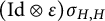
$(\mathrm {Id}\otimes \epsilon )\sigma _{H,H}$
 , and
$\leftharpoonup $
 as
$(\epsilon \otimes \mathrm {Id})\sigma _{H,H}$
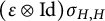 (see [Reference Majid30, p. 300]).
Although there are examples of braidings that are obtained from a pair of actions satisfying (mp.1)–(mp.4) (see Section 5.2), it is not true that all braidings are obtained from a pair of maps as in Remark 2.4:
Counterexample 2.5 Consider, for instance, a coquasitriangular bialgebra
$(H,\mathcal {R})$
 (see Section 5.1) and the usual braiding (5.1) on
${\mathfrak {M}}^H$


If we suppose by contradiction that
$\sigma _{H,H}(a\otimes b) = (a_1\rightharpoonup b_1)\otimes (a_2\leftharpoonup b_2)$
 for some maps
$\rightharpoonup ,\leftharpoonup $
 , then Remark 2.4 yields

but then

and this is generally false. As an example, consider the coquasitriangular structure on the Sweedler’s Hopf algebra described in Section 6.1, with
$a=b=g$
 : one has
$\mathcal {R}(g\otimes g) = -1$
 , whence
$b_1\otimes a_1\mathcal {R}(a_2\otimes b_2) = -g\otimes g$
 and
$\mathcal {R}(a_1\otimes b_2)b_1\otimes a_2\mathcal {R}(a_3\otimes b_3) = g\otimes g$
 , which differ if
 .
Lemma 2.6 (cf. Majid [Reference Majid30, proof of Theorem 7.2.3])
Given a bialgebra H and a morphism
$\sigma _{H,H}:H\otimes H\to H\otimes H$
 satisfying (br.1)–(br.4), the morphisms
$\rightharpoonup \,:= (\mathrm {Id}\otimes \epsilon )\sigma _{H,H}$
 and
$\leftharpoonup \,:=(\epsilon \otimes \mathrm {Id})\sigma _{H,H}$
 are left and right H-actions, respectively.
Proof We compute

and also

The proof is analogous for
$\leftharpoonup $
 .
In general, when
$\sigma _{H,H}$
 does not have the form
$\sigma _{H,H}(x\otimes y)=(x_{1}\rightharpoonup y_{1})\otimes (x_{2}\leftharpoonup y_{2})$
 , the actions
$\rightharpoonup $
 and
$\leftharpoonup $
 defined as in the previous lemma need not form a matched pair, as the following counterexample shows.
Counterexample 2.7 Let us consider again

and the left and right H-actions

Then, we have
$a\rightharpoonup bc=\mathcal {R}(a\otimes b_{2}c_{2})b_{1}c_{1}$
 , while

These are generally distinct (consider for instance the Sweedler’s Hopf algebra in Section 6.1,
$a = b = c=g$
 ,
 ).
2.2 Hopf braces
A skew brace, defined by Guarnieri and Vendramin [Reference Guarnieri and Vendramin18] generalizing Rump [Reference Rump35], is the datum of two group operations on the same set, satisfying a compatibility. Skew braces are ubiquitous in the theory of braidings and the YBE, and hence yearned for a Hopf-theoretic version. This was defined by Angiono, Galindo, and Vendramin [Reference Angiono, Galindo and Vendramin5]:
Definition 2.2 A Hopf brace
$(H,\cdot ,\bullet ,1,\Delta , \epsilon ,S,T)$
 is the datum of two Hopf algebra structures
$(H,\cdot ,1,\Delta ,\epsilon ,S)$
 and
$(H,\bullet ,1',\Delta ,\epsilon ,T)$
 on the same coalgebra
$(H,\Delta ,\epsilon )$
 , satisfying the following compatibility:

Notice that the compatibility condition forces
$1 = 1'$
 (see [Reference Angiono, Galindo and Vendramin5, Remark 1.3]).
When no confusion arises, we shall simply indicate a Hopf brace by
$(H,\cdot , \bullet )$
 . We recall the following characterization.
Proposition 2.8 (Angiono, Galindo and Vendramin [Reference Angiono, Galindo and Vendramin5, Theorems 1.12, 3.3, and Corollary 2.4])
Given a Hopf algebra H, the following data are equivalent:
-
i. a Hopf brace structure $(H,\cdot ,\bullet )$
 on H;
-
ii. a Hopf algebra A, an action $\rightharpoonup $
of A on H such that H is a left A-module algebra, and an isomorphism of coalgebras
$\pi \colon A\to H$
which is a 1-cocycle of bialgebras; i.e.,
$\pi (ab) = \pi (a_1)(a_2\rightharpoonup \pi (b))$
.



In case H is cocommutative, the previous two are also equivalent to
-
iii. a matched pair on H, satisfying the additional condition (⋆).
Moreover, in the cocommutative case,

is a coalgebra isomorphism and a solution to the braid equation on H.
The additional condition (⋆) is the braided commutativity of
$\bullet $
 with respect to the braiding operator
$\sigma _{H,H}$
 .
Remark 2.9 In the cocommutative case, the matched pair obtained from a Hopf brace
$(H,\cdot ,\bullet )$
 is given by
$h\rightharpoonup k=S(h_{1})\cdot (h_{2}\bullet k)$
 and
$h\leftharpoonup k=T(h_{1}\rightharpoonup k_{1})\bullet h_{2}\bullet k_{2}$
 . Then, the corresponding solution of the braid equation is

3 Matched pairs of actions and Yetter–Drinfeld braces
In this section, we generalize the correspondence of Proposition 2.8 by dropping the hypothesis of cocommutativity. As a result, we shall obtain a correspondence between matched pairs of actions on a Hopf algebra, and novel structures which we call Yetter–Drinfeld braces.
3.1 Yetter–Drinfeld braces
Let
$(H,\bullet ,1,\Delta , \epsilon , T) $
 be a Hopf algebra,
$(H,\rightharpoonup ,\leftharpoonup )$
 be a matched pair of actions on H. We begin by defining a second operation
$\cdot $
 and a map
$S\colon H\to H$
 , mimicking [Reference Angiono, Galindo and Vendramin5, Proposition 3.2]:


Notice that
$\bullet $
 is retrieved from
$\cdot $
 as

Recall that the linearity of
$\Delta $
 and
$\epsilon $
 with respect to
$\rightharpoonup $
 read as:

similarly for the linearity of
$\Delta $
 and
$\epsilon $
 with respect to
$\leftharpoonup $
 .
Remark 3.1 The condition (⋆) allows one to retrieve the right action from the left action, and vice versa. Indeed, by the linearity of
$\Delta $
 and
$\epsilon $
 with respect to
$\rightharpoonup $
 , (⋆) is equivalent to

Moreover, (3.4) is clearly equivalent to

From (3.5) one can easily deduce

Remark 3.2 Let us observe that
$S^{2}$
 is given on an element
$a\in H$
 by

Lemma 3.3 One has
$\Delta (a\cdot b) = (a_{1}\bullet (T(a_{3})\rightharpoonup b_{1}))\otimes (a_{2}\cdot b_{2})$
 .
Proof We compute

Although
$\cdot $
 is not a morphism of coalgebras in
 , this will be sorted out by setting ourselves in a suitable category.
An immediate computation shows the form of the twice iterated
$\Delta $
 , which is going to come in handy later:

Proposition 3.4 Let
$(H,\bullet ,1,\Delta ,\epsilon ,T)$
 be a Hopf algebra,
$(H,\rightharpoonup ,\leftharpoonup )$
 a matched pair of actions. Define
$\cdot $
 and S as in (3.1), (3.2). Then,
$(H,\cdot ,1)$
 becomes an algebra,
$\epsilon $
 is a morphism of algebras with respect to this structure, and S satisfies
$a_{1}\cdot S(a_{2})=\epsilon (a)1=S(a_{1})\cdot a_{2}$
 . Moreover, one has

and the two operations
$\bullet $
 and
$\cdot $
 satisfy the Hopf brace compatibility (hbc).
Proof We first observe that

for all
$a\in H$
 . We now prove that
$\cdot $
 is associative. Given
$a,b,c\in H$
 we have:

as desired. We then compute

Moreover, one has

and

As for (3.8), observe that

We finally prove the Hopf brace compatibility (hbc):

As promised, we now reinterpret this additional operation
$\cdot $
 in a suitable category, which is going to be the category of Yetter–Drinfeld modules over H.
Definition 3.1 Let
$(H,\bullet ,1,\Delta , \epsilon , T)$
 be a Hopf algebra. A (left-left) Yetter–Drinfeld module on H is the datum of a left H-module X with an action
$\rightharpoonup \colon H\otimes X\to X$
 , which is also a left H-comodule with a coaction
$\rho \colon X\to H\otimes X$
 , satisfying the following compatibility for all
$x\in X$
 ,
$a\in H$
 :

A morphism of Yetter–Drinfeld modules is a morphism of both left H-modules and left H-comodules. We denote by
$^H_H\mathcal {YD}$
 the category of Yetter–Drinfeld modules over H.
Lemma 3.5 Let
$(H,\bullet ,1,\Delta ,\epsilon ,T)$
 be a Hopf algebra. Suppose that
$\rightharpoonup \colon H\otimes H\to H$
 is a morphism of coalgebras,
$\leftharpoonup \colon H\otimes H\to H$
 is a linear map satisfying
$\epsilon (a\leftharpoonup b)=\epsilon (a)\epsilon (b)$
 , and (⋆) is satisfied. The following conditions are equivalent, and they are all equivalent to (mp.5):


In particular, having a matched pair of actions
$(H,\rightharpoonup ,\leftharpoonup )$
 all the previous equalities hold true.
Proof First, we notice that

Now, we check that (3.10) and (3.9) are equivalent:

We prove that (3.11) and (3.12) are both equivalent to (3.10). One has

and

where we use the fact that (3.10) implies (3.9) and
$\epsilon (a\leftharpoonup b)=\epsilon (a)\epsilon (b)$
 in the latter equivalence. This completes the proof that (3.9)–(3.12) are equivalent. Finally, using the assumption (⋆), (mp.5) clearly implies (3.11); and, conversely, assuming (3.11) (and thus (3.9)) we immediately retrieve (mp.5).
Corollary 3.6 Let
$(H,\bullet ,1,\Delta ,\epsilon ,T)$
 be a Hopf algebra. Every matched pair of actions
$(H,\rightharpoonup ,\leftharpoonup )$
 is a matched pair
$(H,H)$
 on H.
Lemma 3.7 Let
$(H,\rightharpoonup ,\leftharpoonup )$
 be as in the setting of Proposition 3.4. Then,
$(H,\rightharpoonup ,\mathrm {Ad}_{L})$
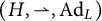 is in
${}^H_H\mathcal {YD}$
 , where
$\mathrm {Ad}_{L}:H\to H\otimes H$
 ,
$a\mapsto a_{1}\bullet T(a_{3})\otimes a_{2}$
 is the left H-adjoint coaction. As a consequence, denoted by
$\sigma ^{\mathcal {YD}}$
 the braiding of
$^H_H\mathcal {YD}$
 , one has that
$\sigma ^{\mathcal {YD}}_{H,H}\colon H\otimes H\to H\otimes H$
 is explicitly described by
$\sigma ^{\mathcal {YD}}_{H,H}\colon a\otimes b\mapsto (a_{1}\bullet T(a_{3})\rightharpoonup b)\otimes a_{2}$
 .
Proof We already know that
$(H,\rightharpoonup )$
 is a left H-module and
$(H,\mathrm {Ad}_{L})$
 is a left H-comodule. Since
$\leftharpoonup $
 is a morphism of coalgebras, the equivalent conditions of Lemma 3.5 hold true. We check the compatibility of Yetter–Drinfeld modules (yd):

Remark 3.8 Notice that the braiding
$\sigma ^{\mathcal {YD}}_{H,H}$
 coincides with the flip map
$\tau $
 in case the adjoint coaction
$\mathrm {Ad}_{L}$
 is trivial, i.e.,
$a_{1}\bullet T(a_{3})\otimes a_{2}=1\otimes a$
 , which clearly happens in the cocommutative case. Conversely, if
$a_{1}\bullet T(a_{3})\otimes a_{2}=1\otimes a$
 , then

and so
$a_{1}\otimes a_{2}=a_{2}\otimes a_{1}$
 , i.e., H is cocommutative. Furthermore, let us also observe that
$\sigma ^{\mathcal {YD}}_{H,H}$
 coincides with
$\tau $
 also in case
$\rightharpoonup $
 is the trivial action.
Proposition 3.9 Let H be a Hopf algebra,
$(B, \cdot , 1_B, \Delta _B, \epsilon _B)$
 a bialgebra in
${}^H_H\mathcal {YD}$
 . Suppose that
$S\colon B\to B$
 is linear map, and a convolution inverse of
$\mathrm {Id}_B$
 : then, B is a Hopf algebra in
$^H_H\mathcal {YD}$
 , with antipode S.
Proof
Footnote
1
Define
$\mathrm {can}\colon B\otimes B \to B\otimes B$
 as
$\mathrm {can}:=(m_{B}\otimes m_{B})(\mathrm {Id}_B\otimes \sigma ^{\mathcal {YD}}_{B,B}\otimes \mathrm {Id}_{B})(\mathrm {Id}_{B}\otimes u_{B}\otimes \Delta _{B}) $
 which is a composition of morphisms in
${}^H_H\mathcal {YD}$
 , and hence a morphism in
${}^H_H\mathcal {YD}$
 . The map
$\mathrm {can}$
 is explicitly given by
$\mathrm {can}(a\otimes b) = (a\cdot b_{1})\otimes b_{2} $
 . Since S is a convolution inverse of
$\mathrm {Id}_{B}$
 ,
$\mathrm {can}$
 is invertible with inverse given by
$\mathrm {can}^{-1}\colon a\otimes b \mapsto (a\cdot S(b_1))\otimes b_2$
 . Since
$\mathrm {can}$
 is invertible and it is a morphism in
$^{H}_{H}\mathcal {YD}$
 , the inverse is also a morphism in
${}^H_H\mathcal {YD}$
 . Now observe that
$S = (\mathrm {Id}_B\otimes \epsilon _B)\mathrm {can}^{-1}(u_B\otimes \mathrm {Id}_B)$
 , thus S is a composition of morphisms in
${}^H_H\mathcal {YD}$
 : thus S is a morphism in
${}^H_H\mathcal {YD}$
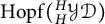
 , and hence B is in
$\mathrm {Hopf}({}^H_H\mathcal {YD})$
 .
We merge the previous results in the following theorem.
Theorem 3.10 Let
$(H,\bullet ,1,\Delta ,\epsilon ,T)$
 be a Hopf algebra,
$(H,\rightharpoonup ,\leftharpoonup )$
 a matched pair of actions. Define
$\cdot $
 and S as in (3.1),(3.2). Then:
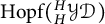
-
i. $(H,\cdot ,1,\Delta ,\epsilon ,S)$
is in
$\mathrm {Hopf}(^{H}_{H}\mathcal {YD})$
with the action
$\rightharpoonup $
and the adjoint coaction
$\mathrm {Ad}_L$
; -
ii. the two operations $\bullet $
and
$\cdot $
satisfy the compatibility condition (hbc).



Proof The compatibility (hbc) is satisfied by Proposition 3.4.
We first check that
$\cdot $
 is a morphism of coalgebras in
$^{H}_{H}\mathcal {YD}$
 . Using Lemma 3.3 we obtain:

i.e.,
$\Delta m_{\cdot }=(m_{\cdot }\otimes m_{\cdot })(\mathrm {Id}\otimes \sigma ^{\mathcal {YD}}_{H,H}\otimes \mathrm {Id})(\Delta \otimes \Delta )$
 . By Proposition 3.4, we also know that
$\epsilon (a\cdot b)=\epsilon (a)\epsilon (b)$
 . Together, they are the compatibility conditions of a bialgebra in
$^{H}_{H}\mathcal {YD}$
 .
Our next step is proving that
$(H,\Delta , \epsilon )$
 is a coalgebra in
$^H_H\mathcal {YD}$
 . We know that
$\Delta $
 and
$\epsilon $
 are left H-linear with respect to
$\rightharpoonup $
 . We thereby prove that they are also left H-colinear. We compute

and

This concludes the proof that
$(H,\Delta ,\epsilon )$
 is a coalgebra in
$^{H}_{H}\mathcal {YD}$
 .
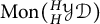
Clearly, the unit  is left H-linear and left H-colinear, so in order to conclude that
$(H,\cdot ,1)$
 is in
$\mathrm {Mon}(^{H}_{H}\mathcal {YD})$
 we only need to verify that
$\cdot $
 is left H-linear and left H-colinear.
First we show that
$\cdot $
 is left H-linear with respect to
$\rightharpoonup $
 . Therefore, we compute

We now check that
$\cdot $
 is left H-colinear with respect to
$\mathrm {Ad}_L$
 . We already know that (3.7) holds, i.e.,

The request that
$\cdot $
 is colinear with respect to the adjoint coaction
$\mathrm {Ad}_L$
 reads as follows:

We now rephrase the condition (3.13). One has

Therefore, (3.13) becomes

But now, using the antipode, we obtain

Thus, we obtain that (3.13) is equivalent to

The latter is implied by (3.12), which holds true since
$\leftharpoonup $
 is a morphism of coalgebras (and is in fact equivalent to (3.12) when T is bijective). This concludes the proof that
$(H,\cdot , 1)$
 is an algebra in
$^H_H\mathcal {YD}$
 , and hence
$(H,\cdot , 1,\Delta , \epsilon )$
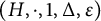 is a bialgebra in
$^H_H\mathcal {YD}$
 for what already observed.
We already know from Proposition 3.4 that S satisfies
$S(a_1)\cdot a_2 = \epsilon (a)1_{H}= a_1\cdot S(a_2)$
 , thus we only need to prove that S is a morphism of Yetter–Drinfeld modules. This follows from Proposition 3.9.
Definition 3.2 Given a matched pair
$(H, \rightharpoonup , \leftharpoonup )$
 on a Hopf algebra
$(H,\bullet , 1, \Delta , \epsilon , T)$
 , the second structure
 from Theorem 3.10 i. will be called the transmutation of
$H^\bullet $
 with respect to the matched pair.
In Remark 5.6, we shall see that this is indeed a generalization of Majid’s transmutation [Reference Majid28].
Remark 3.11 By [Reference Andruskiewitsch and Schneider4, Remark 1.8] the Hopf algebra
$(H,\cdot ,1,\Delta , \epsilon , S)$
 is, in particular, a braided Hopf algebra in the sense of Kharchenko [Reference Kharchenko22, Section 2.2]. If moreover T is bijective, then the braiding
$\sigma ^{\mathcal {YD}}$
 is bijective, hence
$(H,\cdot ,1,\Delta , \epsilon , S)$
 is a braided Hopf algebra in the sense of Majid [Reference Majid29]; see also [Reference Takeuchi39, Definition 5.1].
Remark 3.12 In case H is cocommutative,
$\sigma ^{\mathcal {YD}}_{H,H}$
 coincides with the flip
$\tau $
 , hence
$(H,\cdot ,1,\Delta ,\epsilon ,S)$
 becomes a standard Hopf algebra and we recover the definition of Hopf brace [Reference Angiono, Galindo and Vendramin5].
Corollary 3.13 Let
$(H,\bullet ,1,\Delta ,\epsilon ,T)$
 be a Hopf algebra and
$(H,\rightharpoonup ,\leftharpoonup )$
 a matched pair of actions. Define
$\cdot $
 as in (3.1), and S as in (3.2). Then, the following is a bialgebra structure on
$H\otimes H$
 :

Proof Let
$H^\bullet :=(H,\bullet )$
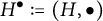 and
 denote the two multiplicative structures. By Theorem 3.10, we have that
$(H,\cdot ,1,\Delta ,\epsilon )$
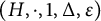 is in
$\mathrm {Bimon}({}^{H}_{H}\mathcal {YD})$
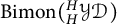 , thus the bosonization
 is a bialgebra, where
$(a\otimes h)\cdot _{\#}(a'\otimes h'):=a\cdot (h_{1}\rightharpoonup a')\otimes h_{2}\bullet h'$
 and
$\Delta _{\#}(a\otimes h):=a_{1}\otimes a_{2_{-1}}\bullet h_{1}\otimes a_{2_{0}}\otimes h_{2}$
 denote the smash product and the smash coproduct, respectively, see e.g., Heckenberger and Schneider [Reference Heckenberger and Schneider19, Proposition 3.8.4]. Moreover, since
$H^{\bullet }$
 and
 are both Hopf algebras, we obtain an antipode on
 given by
$S_{\#}(a\otimes h):=\big (T(a_{-1}\bullet h_{2})\rightharpoonup S(a_{0})\big )\otimes T(a_{-2}\bullet h_{1})$
 ; see e.g., [Reference Heckenberger and Schneider19, Theorem 3.8.10]. Thus, we compute

Theorem 3.10 suggests us the following definition.
Definition 3.3 A Yetter–Drinfeld brace (or
$\mathcal {YD}$
 -brace)
$(H, \cdot , \bullet ,1,\Delta ,\epsilon ,S,T)$
 is the datum of a Hopf algebra
$H^\bullet = (H,\bullet , 1,\Delta , \epsilon , T)$
 , a second operation
$\cdot $
 on H, and a linear map
$S\colon H\to H$
 such that:
-
i. $(H,\cdot ,1,\Delta ,\epsilon ,S)$
is in
$\mathrm {Hopf}({}^{H^\bullet }_{H^\bullet }\mathcal {YD})$
with the action
$\rightharpoonup $
defined by
$a\rightharpoonup b := S(a_1)\cdot (a_2\bullet b)$
, and the coaction given by
$\mathrm {Ad}_L$
; -
ii. if we define $a\leftharpoonup b:= T(a_1\rightharpoonup b_1)\bullet a_2\bullet b_2$
, the two maps
$\rightharpoonup , \leftharpoonup $
satisfy (mp.5); -
iii. the two operations $\bullet $
and
$\cdot $
satisfy the Hopf brace compatibility (hbc).

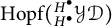






Given two Yetter–Drinfeld braces H and K, a morphism of Yetter–Drinfeld braces is a map
$f\colon H\to K$
 that is a morphism in
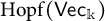 between the respective Hopf algebras in
 , and satisfies

In particular, this implies
$S_{K}f=fS_{H}$
 ,
$f\rightharpoonup _{H}\;=\;\rightharpoonup _{K}\!(f\otimes f)$
 and
$(\mathrm {Ad}_{L})_Kf=(f\otimes f)(\mathrm {Ad}_{L})_H$
 . We denote the category of Yetter–Drinfeld braces by
 .
Remark 3.14 Let
$f\colon H\to K$
 be a morphism of Yetter–Drinfeld braces. Since
$f\colon H^{\bullet }\to K^{\bullet }$
 is a morphism of bialgebras, one can regard
 as a left
$H^{\bullet }$
 -module through f, so that the condition
$f(a\rightharpoonup _{H} b)=f(a)\rightharpoonup _{K}f(b)$
 means that f is a morphism in
$_{H^{\bullet }}\mathfrak {M}$
 ; and
 as a left
$K^{\bullet }$
 -comodule through f, so that the condition
$(\mathrm {Ad}_{L})_{K}f=(f\otimes f)(\mathrm {Ad}_{L})_{H}$
 means that f is a morphism in
$^{K^{\bullet }}\mathfrak {M}$
 . One can consider the category
$^{K^{\bullet }}_{H^{\bullet }}\mathcal {YD}$
 of relative Yetter–Drinfeld modules; see [Reference Caenepeel, Militaru and Zhu8, Section 4.4, p. 183]. Clearly
 and
 are in
$^{K^{\bullet }}_{H^{\bullet }}\mathcal {YD}$
 . Indeed, given
$a,b\in H$
 , we compute:

where
$a_{-1}\otimes a_0 = (\mathrm {Ad}_L)_H(a)$
 is the usual adjoint
$H^\bullet $
 -coaction on H, while
$a^K_{-1}\otimes a^K_0= (f\otimes \mathrm {Id})(\mathrm {Ad}_L)_H(a)$
 denotes the
$K^\bullet $
 -coaction on
 induced by
$\mathrm {Ad}_L$
 through f. The Yetter–Drinfeld compatibility for
 is deduced analogously. Hence, we obtain that f is a morphism in
$^{K^{\bullet }}_{H^{\bullet }}\mathcal {YD}$
 . Moreover, one clearly has that
 and
 are in
$\mathrm {Mon}(^{K^{\bullet }}_{H^{\bullet }}\mathcal {YD})$
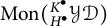 and
$\mathrm {Comon}(^{K^{\bullet }}_{H^{\bullet }}\mathcal {YD})$
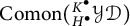 ; thus the condition
$f(a\cdot _{H}b)=f(a)\cdot _{K}f(b)$
 means that
 is a morphism in
$\mathrm {Mon}(^{K^{\bullet }}_{H^{\bullet }}\mathcal {YD})$
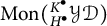 . Notice that
$f $
 is automatically a morphism in
$\mathrm {Comon}(^{K^{\bullet }}_{H^{\bullet }}\mathcal {YD})$
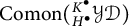 .
From Theorem 3.10, we obtain:
Corollary 3.15 Let
$(H,\bullet ,1,\Delta ,\epsilon ,T)$
 be a Hopf algebra,
$(H,\rightharpoonup ,\leftharpoonup )$
 a matched pair of actions. Define
$\cdot $
 and S as in (3.1), (3.2). Then,
$(H,\cdot ,\bullet ,1,\Delta ,\epsilon ,S,T)$
 is a Yetter–Drinfeld brace.
Remark 3.16 Define
$\leftharpoonup $
 as in Definition 3.3 ii. Since
$\rightharpoonup $
 is a morphism of coalgebras, it is clear that
$\rightharpoonup , \leftharpoonup $
 satisfy (⋆):

Observe that
$\epsilon (a\leftharpoonup b) = \epsilon (a)\epsilon (b)$
 , thus we are in the hypotheses of Lemma 3.5. Consequently, Definition 3.3 ii. is equivalent to the request that
$\leftharpoonup $
 is a morphism of coalgebras.
Remark 3.17 Notice that Definition 3.3 makes as much sense when we replace  with a braided monoidal category. Although this exceeds the scope of this work, we may expect several of our results in
 to hold more in general. Furthermore, Definition 3.3 can be dualized to define Yetter–Drinfeld cobraces, leading to a generalization of commutative Hopf cobraces [Reference Angiono, Galindo and Vendramin5].
Clearly, in a Yetter–Drinfeld brace, the map
$\rightharpoonup $
 defined as in Definition 3.3 i. is a left
$H^{\bullet }$
 -action, and
$(H,\cdot ,1)$
 is a left
$H^{\bullet }$
 -module algebra. In fact, this is true under weaker assumptions:
Lemma 3.18 Let
$H^\bullet =(H,\bullet ,1,\Delta ,\epsilon )$
 be a bialgebra and
$(H,\cdot ,1,\Delta ,\epsilon )$
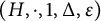 be an algebra and a coalgebra, endowed with a map
$S\colon H\to H$
 satisfying
$S(a_{1})\cdot a_{2}=\epsilon (a)1=a_{1}\cdot S(a_{2})$
 . Suppose that the Hopf brace compatibility (hbc) between
$\bullet $
 and
$\cdot $
 is satisfied. Then

is a left
$H^{\bullet }$
 -action on H. Moreover,
$(H,\cdot ,1)$
 is a left
$H^{\bullet }$
 -module algebra and, if
$\epsilon $
 is a morphism of algebras with respect to
$\cdot $
 , then
$\epsilon $
 is left
$H^{\bullet }$
 -linear with respect to
$\rightharpoonup $
 .
Proof First we compute
$1\rightharpoonup b=S(1)\cdot (1\bullet b)=b$
 . Moreover, we have

where the equality marked with
$(\dagger )$
 follows from the relation
$S(a_{1}\bullet b)\cdot a_{2}=S(a_{1})\cdot (a_{2}\bullet S(b))$
 , whose proof is the same as in [Reference Angiono, Galindo and Vendramin5, Lemma 1.7] and simply follows from (hbc). Moreover, we have

and

hence
$(H,\cdot ,1)$
 is a left
$H^{\bullet }$
 -module algebra. Finally, we have

where
$(\ddagger )$
 follows from the fact that
$\epsilon $
 is a morphism of algebras with respect to
$\cdot $
 .
3.2 A general example
We now construct an easy example of a Yetter–Drinfeld brace on a Hopf algebra H. This construction depends on the assumption that the adjoint action on H is compatible with the comultiplication.
Lemma 3.19 Let
$H^{\bullet }:=(H,\bullet ,1,\Delta ,\epsilon ,T)$
 be a Hopf algebra,
$\rightharpoonup $
 the left adjoint action
$a\rightharpoonup b:=a_{1}\bullet b\bullet T(a_{2})$
 , and
$\leftharpoonup $
 the trivial action. Then,
$(H,\rightharpoonup ,\leftharpoonup )$
 is a matched pair of actions if and only if
$\Delta $
 is left linear with respect to
$\rightharpoonup $
 .
Proof Notice that
$H^{\bullet }$
 is automatically a right H-module coalgebra. We verify (mp.1)–(mp.4) and (⋆). Clearly
$a\rightharpoonup 1=\epsilon (a)1$
 holds, while (mp.2) is automatically true. Moreover, we compute

and

Finally,

Thus,
$(H,\rightharpoonup ,\leftharpoonup )$
 is a matched pair of actions if and only if
$H^{\bullet }$
 is a left H-module coalgebra. Since
$\epsilon (a\rightharpoonup b)=\epsilon (a)\epsilon (b)$
 is automatically satisfied,
$H^\bullet $
 is a left H-module coalgebra if and only if
$\Delta $
 is left linear with respect to
$\rightharpoonup $
 ; as desired.
Remark 3.20 The linearity condition of
$\Delta $
 with respect to
$\rightharpoonup $
 , i.e.,
$\Delta (a\rightharpoonup b)=(a_{1}\rightharpoonup b_{1})\otimes (a_{2}\rightharpoonup b_{2})$
 , explicitly reads:

The latter is equivalent to
$T(a_{3})\otimes a_{1}\bullet b\bullet T(a_{2})=T(a_{1})\otimes a_{2}\bullet b\bullet T(a_{3})$
 , and then to

i.e.,
$(\mathrm {Id}\otimes \rightharpoonup )(\mathrm {Ad}_{L}\otimes \mathrm {Id})=(u_{H}\otimes \mathrm {\rightharpoonup })$
 , where
$\mathrm {Ad}_{L}$
 denotes again the left adjoint coaction on H. From the matched pair of actions
$(H,\rightharpoonup ,\leftharpoonup )$
 of Lemma 3.19, we can define
$\cdot $
 as in (3.1), and S as in (3.2), obtaining

Notice that (3.17) clearly holds in the commutative and cocommutative cases (where the latter was already considered, e.g., in Masuoka [Reference Masuoka32, Remark p. 302]). If
$H^{\bullet }$
 is commutative, then
$(H,\bullet ,\bullet )$
 is an example of a Yetter–Drinfeld brace. On the other hand, if
$H^{\bullet }$
 is cocommutative, then the previous construction reduces to the almost trivial Hopf brace
$(H,\bullet ^{\mathrm {op}},\bullet )$
 (the terminology is adapted from [Reference Guarnieri and Vendramin18]).
In Section 5, we shall see other explicit examples coming from coquasitriangular structures. In particular, the first example will be the Sweedler’s Hopf algebra
$H_4$
 . Generalizations of
$H_4$
 are given by the Taft algebras
$H_{n^{2}}$
 , which do not admit any (co)quasitriangular structure for
$n>2$
 (see Gelaki [Reference Gelaki17]). Matched pairs
$(H_{n^{2}},H_{n^{2}})$
 on
$H_{n^{2}}$
 are classified by Agore [Reference Agore1, Theorem 2.1], and it is not difficult to see that none of these matched pairs satisfy (⋆). This explicitly shows that matched pairs of actions
$(H,\rightharpoonup ,\leftharpoonup )$
 correspond to a proper subclass of the matched pairs
$(H,H)$
 on H.
3.3 A converse connection
In order to show that our definition of Yetter–Drinfeld braces is optimal, we now prove that the correspondence of Theorem 3.10 has a converse. Therefore, a Yetter–Drinfeld brace and a matched pair of actions are essentially the same thing. This is in fact, as we shall point out, an isomorphism of categories.
Theorem 3.21 Let
$(H,\cdot , \bullet , 1, \Delta , \epsilon , S, T)$
 be a Yetter–Drinfeld brace. Define

Then,
$(H,\rightharpoonup ,\leftharpoonup )$
 is a matched pair of actions.
Proof Since H is in
$\mathrm {Comon}({}^{H^\bullet }_{H^\bullet }\mathcal {YD})$
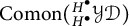 , one has that
$\Delta $
 and
$\epsilon $
 are left
$H^\bullet $
 -linear with respect to
$\rightharpoonup $
 , and hence H is a left
$H^\bullet $
 -module coalgebra. From the definition of
$\rightharpoonup $
 we immediately have
$a\bullet b = a_1\cdot S(a_2)\cdot (a_3\bullet b) = a_1\cdot (a_2\rightharpoonup b)$
 , whence also

We therefore compute

Moreover, we have
$a\leftharpoonup 1=T(a_{1}\rightharpoonup 1)\bullet a_{2}\bullet 1=T(\epsilon (a_{1})1)\bullet a_{2}=a$
 , thus
$\leftharpoonup $
 is a right
$H^{\bullet }$
 -action. By Remark 3.16, we already know that
$\Delta $
 is right
$H^{\bullet }$
 -linear with respect to
$\leftharpoonup $
 , i.e.,
$\Delta (a\leftharpoonup b) = (a_1\leftharpoonup b_1)\otimes (a_2\leftharpoonup b_2)$
 ; that H is a right
$H^\bullet $
 -module coalgebra, and that (⋆) is satisfied. We already know that (mp.1) is satisfied. Moreover, (mp.2) also holds:

In order to show that
$(H,\rightharpoonup ,\leftharpoonup )$
 is a matched pair of actions on H, it remains to prove that (mp.3) and (mp.4) are satisfied. We thereby compute

where
$(\dagger )$
 follows since
$(H,\cdot ,1)$
 is a left
$H^{\bullet }$
 -module algebra. Finally, one has

The previous construction is converse to the one of Theorem 3.10.
Theorem 3.22 The correspondence established in Theorems 3.10 and 3.21 is an isomorphism between  and
 .
Proof Since the constructions of Theorems 3.10 and 3.21 are converse to each other, if we prove that these constructions are functorial then they automatically yield an isomorphism of categories.
Let  be the assignment defined in Theorem 3.10. We define the assignment on morphisms as follows: if
$f\colon (H,\rightharpoonup _H,\leftharpoonup _H)\to (K,\rightharpoonup _K,\leftharpoonup _K)$
 is a morphism in
 , the corresponding morphism in
 is
$f\colon H\to K$
 read as a morphism of Hopf algebras. Since
$m_{\cdot _{H}} = m_{\bullet _{H}}(\mathrm {Id}_{H}\otimes \rightharpoonup _{H})(\mathrm {Id}_{H}\otimes T_{H}\otimes \mathrm {Id}_{H})(\Delta _{H}\otimes \mathrm {Id}_{H})$
 (and a similar formula holds for
$m_{\cdot _{K}}$
 ), one has

thus f is indeed a morphism in  . Moreover, it is clear that F sends the identity morphism into the identity morphism. Finally, let
$f\colon (H,\rightharpoonup _H,\leftharpoonup _H)\to (K,\rightharpoonup _K,\leftharpoonup _K)$
 and
$g\colon (K,\rightharpoonup _K,\leftharpoonup _K)\to (L,\rightharpoonup _L,\leftharpoonup _L) $
 be morphisms in
 , then F sends the composition
$gf$
 in
 into the set-theoretic composition of maps
$gf$
 , which is the composition of morphisms in
 .
Analogously, one proves that the assignment  defined in Theorem 3.21 is a functor.
4 Yetter–Drinfeld braces as 1-cocycles
It is known (see Angiono, Galindo, and Vendramin [Reference Angiono, Galindo and Vendramin5, Theorem 1.12], and Fernández Vilaboa and Gonzáles Rodríguez [Reference Fernández Vilaboa, González Rodríguez, Ramos Pérez and Rodríguez Raposo15, Theorem 2.7]) that a Hopf brace in a braided monoidal category
$\mathcal {M}$
 is tantamount to a 1-cocycle of bialgebras in
$\mathcal {M}$
 . We are going to recover an analogous characterization for Yetter–Drinfeld braces.
Definition 4.1 Let
$(H,\bullet ,1,\Delta ,\epsilon ,T)$
 be a Hopf algebra,
$(A,\cdot _{A},1,\Delta ,\epsilon )$
 be a bialgebra in
$^H_H\mathcal {YD}$
 , and let the action of H on A be denoted by
$\rightharpoonup _{A}$
 . A Yetter–Drinfeld 1-cocycle is an isomorphism of coalgebras
$\pi \colon H\to A$
 satisfying the 1-cocycle condition

and satisfying the following conditions for all
$a,b\in H$
 :


Given two Yetter–Drinfeld 1-cocycles
$\pi \colon H\to A $
 and
$\varpi \colon K\to B$
 , a morphism of Yetter–Drinfeld 1-cocycles
$\pi \to \varpi $
 is a pair
$(f,g)$
 , where
$f\colon H\to K$
 is a morphism of Hopf algebras, and
$g\colon A\to B$
 is a morphism of algebras and coalgebras satisfying

We denote by  the category of Yetter–Drinfeld 1-cocycles thus obtained.
Remark 4.1 Observe that, choosing
$a=b=1_{H}$
 in (1c), we obtain
$\pi (1_{H})=\pi (1_{H})\cdot _{A}\pi (1_{H})$
 . Moreover, taking
$a=1_{H}$
 in (4.1), we obtain
$\pi (1_{H})\cdot _{A}\pi (1_{H})=1_{A}$
 . Hence

is automatically satisfied. The same is true for 1-cocycles of Hopf algebras [Reference Angiono, Galindo and Vendramin5].
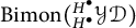
Theorem 4.2 Let
$H^{\bullet }:=(H,\bullet ,1,\Delta ,\epsilon ,T)$
 be a Hopf algebra. The following data are equivalent:
-
i. a coalgebra A and an isomorphism of coalgebras $\pi :H\to A$
, such that A with the coaction
$\rho :=(\mathrm {Id}\otimes \pi )\mathrm {Ad}_{L}\pi ^{-1}$
is in
$\mathrm {Bimon}(^{H^{\bullet }}_{H^{\bullet }}\mathcal {YD})$
, and
$\pi $
is a Yetter–Drinfeld 1-cocycle; -
ii. a second operation $\cdot $
and a map S, providing a Yetter–Drinfeld brace structure on H.




This defines an equivalence of categories between the subcategory of  given by Yetter–Drinfeld 1-cocycles
$\pi :H\to A$
 where A has coaction
$(\mathrm {Id}\otimes \pi )\mathrm {Ad}_{L}\pi ^{-1}$
 and
 .
Proof The proof is fundamentally the same as for Hopf braces [Reference Angiono, Galindo and Vendramin5, Theorem 1.12].
i. to ii.
Suppose given a Yetter–Drinfeld 1-cocycle
$\pi \colon H\to A$
 . Define the second structure
 on H by pulling back the multiplication
$\cdot _{A}$
 of A:

This is clearly associative and, from (4.3), it is immediate that  is unitary with unit
$1_H$
 . Define
$S(a):= \pi ^{-1}(a_1\rightharpoonup _A \pi T(a_2))$
 , and consequently let

In particular S satisfies
$S(a) = a_1\rightharpoonup T(a_2)$
 , which is (3.2). Since
$\rightharpoonup $
 is just the action
$\rightharpoonup _A$
 pulled back through
$\pi $
 , this is clearly a left action of
$H^\bullet $
 on itself. By assumption, A is in
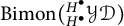
$\mathrm {Bimon}(^{H^{\bullet }}_{H^{\bullet }}\mathcal {YD})$
 with coaction
$\rho (a)=(\mathrm {Id}\otimes \pi )\mathrm {Ad}_{L}\pi ^{-1}(a)=\pi ^{-1}(a_{1})\bullet T(\pi ^{-1}(a_{3}))\otimes a_{2}$
 , hence
$\rho $
 and
$\rightharpoonup $
 satisfy the compatibility condition of a Yetter–Drinfeld module:

moreover
$\cdot _A$
 and
$\Delta $
 satisfy the bialgebra compatibility in
$^{H^{\bullet }}_{H^{\bullet }}\mathcal {YD}$
 :

It easily follows that  is in
$^{H^{\bullet }}_{H^{\bullet }}\mathcal {YD}$
 , and that
$m_{\cdot }$
 , u,
$\Delta $
 and
$\epsilon $
 are left linear with respect to
$\rightharpoonup $
 .
We show that S is a convolution inverse of
$\mathrm {Id}_H$
 with respect to the algebra structure
 :

and

Let
$a\leftharpoonup b:=T(a_{1}\rightharpoonup b_{1})\bullet a_{2}\bullet b_{2}=T\pi ^{-1}(a_{1}\rightharpoonup _{A}\pi (b_{1}))\bullet a_{2}\bullet b_{2}$
 . Notice that (3.5) is automatically satisfied. We verify that
$\leftharpoonup $
 satisfies (3.9):

Moreover, since
$\epsilon (a\rightharpoonup b)=\epsilon (a)\epsilon (b)$
 , one clearly has
$\epsilon (a\leftharpoonup b)=\epsilon (a)\epsilon (b)$
 , hence
$\leftharpoonup $
 is a morphism of coalgebras: by Remark 3.16, this is equivalent to requiring (mp.5). Furthermore,
$(a_1\rightharpoonup b_1)\bullet (a_2\leftharpoonup b_2) = a\bullet b$
 holds by definition. By Lemma 3.5, we have that (3.12) is satisfied.
Moreover, one has

and this implies (hbc) because
$\pi $
 is bijective.
In order to obtain that  is in
$\mathrm {Bimon}(^{H^{\bullet }}_{H^{\bullet }}\mathcal {YD})$
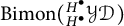 , it remains to prove that
$\Delta $
 is a morphism of algebras with respect to
$\cdot $
 in
$^{H^{\bullet }}_{H^{\bullet }}\mathcal {YD}$
 , and that
$m_{\cdot }$
 is left colinear with respect to
$\mathrm {Ad}_{L}$
 . Both easily follow from the analogous properties of A.
Finally, by Proposition 3.9, we obtain that S is an antipode for  . Thus,
$(H,\cdot ,\bullet ,1,\Delta ,\epsilon ,S,T)$
 is a Yetter–Drinfeld brace.
ii. to i.
Suppose given a Yetter–Drinfeld brace
$(H,\cdot ,\bullet ,1,\Delta ,\epsilon , S,T)$
 . Define
${A:=(H,\cdot , 1,\Delta ,\epsilon )}$
 . This is in
$\mathrm {Bimon}(^{H^{\bullet }}_{H^{\bullet }}\mathcal {YD})$
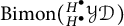 with action
$a\rightharpoonup b=S(a_{1})\cdot (a_{2}\bullet b)$
 , and the coaction
$\mathrm {Ad}_{L}$
 . Set
 , which is clearly a coalgebra isomorphism. Moreover, we compute

while (4.1) and (4.2) are automatically satisfied. Thus  is a Yetter–Drinfeld 1-cocycle.
Functoriality. We verify that the above correspondence is functorial. Let
$\pi \colon H\to A$
 ,
$\varpi \colon K\to B$
 be Yetter–Drinfeld 1-cocycles, with a morphism
$\pi \to \varpi $
 in
 given by maps
$f\colon H\to K$
 ,
$g\colon A\to B$
 . Then
$f\colon H^\bullet \to K^\bullet $
 is a morphism of Hopf algebras. Moreover,

and

thus f is a morphism in  . The above construction clearly sends identity morphisms into identity morphisms, and respects the composition of maps. We denote by F the functor
 thus obtained.
Conversely, a functor  is defined by the following action on the maps: if
$f\colon H\to K$
 is a morphism of Yetter–Drinfeld braces, let
$Gf$
 be the pair of maps
$(f,f)$
 , where the former is interpreted as a map
$f\colon H^\bullet \to K^\bullet $
 , and the latter as a map
 . We check that this is a morphism in
 between
 and
 .
We already know that
$f:H^{\bullet }\to K^{\bullet }$
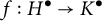 is a morphism of Hopf algebras and
 is a morphism of algebras and coalgebras. Moreover,
$f(a\rightharpoonup _H b) = f(a)\rightharpoonup _H f(b)$
 holds true because f is a morphism in
 . The assignment G clearly respects identities and compositions.
Equivalence. We finally check that this is an equivalence of categories. It is clear that
$FG$
 is the identity functor. Given a Yetter–Drinfeld 1-cocycle
$\pi \colon H^{\bullet }\to A$
 , one has that
$GF(\pi )$
 is the Yetter–Drinfeld 1-cocycle
 , which is isomorphic to
$\pi \colon H^{\bullet }\to A$
 via the morphism
$(\mathrm {Id}_H,\pi ^{-1})$
 . It is easy to verify that this is indeed a morphism in
 , and its inverse is clearly
$(\mathrm {Id}_H, \pi )$
 .
5 Coquasitriangular Hopf algebras and Yetter–Drinfeld braces
In this section, we shall prove that coquasitriangular bialgebras H yield matched pairs of actions
$(H,\rightharpoonup ,\leftharpoonup )$
 satisfying the hypotheses of Theorem 3.10, and hence enable us to construct concrete examples of Yetter–Drinfeld braces. The additional structure, here, coincides with Majid’s transmutation of H [Reference Majid28].
5.1 Coquasitriangular bialgebras
The notion of quasitriangular bialgebra was introduced by Drinfeld [Reference Drinfeld11], to relax the hypothesis of cocommutativity. Here we shall operate with the dual notion, which appeared in several works in between 1990 and 1993, such as in Schauenburg [Reference Schauenburg36], Doi [Reference Doi10], Larson and Towber [Reference Larson and Towber23], and Majid [Reference Majid27].
Definition 5.1 A coquasitriangular bialgebra, denoted by
$(H,m,u,\Delta ,\epsilon , \mathcal {R})$
 or simply by
$(H,\mathcal {R})$
 , is the datum of a bialgebra
$(H,m,u,\Delta ,\epsilon )$
 and of a convolution-invertible morphism
 , satisfying:


Moreover,
$(H,\mathcal {R})$
 is called cotriangular if
$\mathcal {R}^{-1}=\mathcal {R}^{\mathrm {op}}$
 , where
$\mathcal {R}^{-1}$
 denotes the convolution inverse of
$\mathcal {R}$
 .
If
$\mathcal {R}$
 provides a coquasitriangular structure, then the convolution inverse
$\mathcal {R}^{-1}$
 satisfies:


Let
$\mathcal {R}$
 be a coquasitriangular structure on a bialgebra H. Then, it is known that
$\mathcal {R}$
 and its convolution inverse
$\mathcal {R}^{-1}$
 satisfy the quantum YBE (see [Reference Majid30, Lemma 2.2.3]):

Moreover, if H is a Hopf algebra with antipode S, then the following relations hold true:


see [Reference Majid30, Lemma 2.2.2]. It is well known that a bialgebra H is coquasitriangular if and only if the category
${\mathfrak {M}}^{H}$
 of right H-comodules is braided (see [Reference Majid30, Exercise 9.2.9] and the considerations following [Reference Majid30, Theorem 9.2.4]). Indeed, given a coquasitriangular structure
$\mathcal {R}$
 , the bialgebra H becomes a braided object with the braiding operator

and a braiding on
${\mathfrak {M}}^{H}$
 is defined for all
$X,Y$
 in
${\mathfrak {M}}^{H}$
 by setting

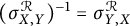
Moreover, H is cotriangular if and only if the category
${\mathfrak {M}}^{H}$
 is symmetric, i.e.,
$(\sigma ^{\mathcal {R}}_{X,Y})^{-1}=\sigma ^{\mathcal {R}}_{Y,X}$
 for all
$X,Y$
 in
${\mathfrak {M}}^{H}$
 .
In the rest of this section, however, we shall use another braiding operator on H. Let
$(H,\mathcal {R})$
 be a coquasitriangular bialgebra, then the map
$\sigma _{H,H}\colon H\otimes H\to H\otimes H$
 defined by

is known to be a braiding operator on H, with inverse given by

Moreover,
$m_{H}\sigma _{H,H}= m_{H}$
 holds.
Remark 5.1 The braiding operator (5.2) extends to a braiding

on the category of bicomodules
$^H{\mathfrak {M}}^H$
 . However, the braidings on
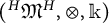 are not yet classified, and the problem is seemingly hard. When the category of bimodules
${}_H{\mathfrak {M}}_H$
 is endowed with the tensor product
$\otimes _H$
 instead of
 , however, a classification was found by Agore, Caenepeel, and Militaru [Reference Agore, Caenepeel and Militaru2], which could be dualized for the category
$^{H}{\mathfrak {M}}^{H}$
 .
Remark 5.2 Let
$\sigma _{H,H}$
 be the braiding operator defined in (5.2). Notice that

hence we have that
$\sigma _{H,H}^{2}=\mathrm {Id}_{H\otimes H}$
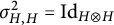 if and only if
$\mathrm {Id}_{H\otimes H}*(\mathcal {R}^{\mathrm {op}}*\mathcal {R})=(\mathcal {R}^{\mathrm {op}}*\mathcal {R})*\mathrm {Id}_{H\otimes H}$
 . The element
$\mathcal {R}^{\mathrm {op}} *\mathcal {R}$
 is also known as the quantum Killing form. In particular, if
$\mathcal {R}^{\mathrm {op}}=\mathcal {R}^{-1}$
 , one clearly has
$\sigma ^{-1}_{H,H}=\sigma _{H,H}$
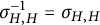 .
5.2 Coquasitriangular Hopf algebras and matched pairs of actions
Suppose given a coquasitriangular Hopf algebra
$(H,\bullet , 1,\Delta ,\epsilon , T,\mathcal {R})$
 . We shall see that the braiding operator (5.2) yields a matched pair satisfying (⋆), and hence a Yetter–Drinfeld brace. The product and the antipode of the corresponding Hopf algebra structure in
$^H_H\mathcal {YD}$
 coincide with those obtained by transmutation of H, introduced by Majid [Reference Majid28]; thus providing a Yetter–Drinfeld brace-theoretic interpretation of the theory of transmutation. At the end of this section, we shall also observe that the same construction cannot be carried out with the braiding (5.1).
Let
$\sigma _{H,H}$
 be defined as in (5.2), and define


These are a left and a right action respectively, by Lemma 2.6, and H becomes a left and right module coalgebra with the respective actions. Moreover, these actions provide a matched pair
$(H,H)$
 , see [Reference Majid30, Example 7.2.7]. Observe that the braiding (5.2) is retrieved as

Hence the fact that
$(H,\rightharpoonup ,\leftharpoonup )$
 satisfies (mp.1)–(mp.4) can also be obtained using Lemmas 2.2 and 2.3, while (⋆) is immediate.
Remark 5.3 The bialgebra
$H \bowtie H$
 described in Section 2, when the matched pair is derived as in (5.3) and (5.4), is denoted in Majid [Reference Majid30] by
$H\bowtie _{\mathcal {R}}H$
 . This has product given by

Moreover, we have

so this situation falls under the hypotheses of [Reference Majid30, Lemma 7.4.8] where, in our case, the coaction is given by
$\mathrm {Ad}_{R}\colon a\mapsto a_{2}\otimes T(a_{1})\bullet a_{3}$
 . Thus [Reference Majid30, Lemma 7.4.8] ensures us that H is also a right H-module with respect to
$\leftharpoonup $
 . Hence, using
$\leftharpoonup $
 and
$\mathrm {Ad}_{R}$
 one can construct the bialgebra
 (we borrow the notation from [Reference Majid30]), where
$\underline {H}$
 is the (right) transmutation of H [Reference Majid30, Theorem 7.4.1] (see also [Reference Majid30, Example 9.4.10]), and the symbol
 denotes the bialgebra with smash product algebra structure, and smash coproduct coalgebra structure. So
 is exactly the bosonization
$H\#\underline {H}$
 , built using the right action and the right coaction. By [Reference Majid30, Theorem 7.4.10], one also obtains an isomorphism
 . In Remark 5.6, we shall relate
 with a left version
$\overline {H}$
 of Majid’s transmutation.
Notice that

In this case, (3.1) takes the following form:

and also

while (3.2) has the following form:

Remark 5.4 When H is cocommutative,
$\rightharpoonup $
 is trivial, and hence
$\cdot $
 coincides with
$\bullet $
 . Thus the corresponding Yetter–Drinfeld brace is just the trivial Hopf brace
$(H,\bullet ,\bullet )$
 (the terminology is again adapted from [Reference Guarnieri and Vendramin18]).
Theorem 5.5 Let
$(H,\bullet ,1,\Delta ,\epsilon ,T, \mathcal {R})$
 be a coquasitriangular Hopf algebra. Define
$\rightharpoonup $
 and
$\leftharpoonup $
 as above, and define
$\cdot $
 and S accordingly. Then,
$(H,\cdot ,\bullet ,1,\Delta ,\epsilon , S,T)$
 is a Yetter–Drinfeld brace. Furthermore, if
$\mathcal {R}$
 is cotriangular, then
$\cdot $
 is braided-commutative with respect to the braiding of
$^H_H\mathcal {YD}$
 , whence also
$S^{2}=\mathrm {Id}_{H}$
 .
Proof We already know that
$(H,\rightharpoonup ,\leftharpoonup )$
 satisfies (mp.1)–(mp.4) [Reference Majid30, Example 7.2.7]. Moreover, it follows from (coqt.1) that H is braided-commutative, i.e.,
$m_\bullet \sigma _{H,H} = m_\bullet $
 , which translates into condition (⋆). Corollary 3.15 yields that
$(H,\cdot ,\bullet ,1,\Delta ,\epsilon ,S,T)$
 is a Yetter–Drinfeld brace.
Suppose now that
$\mathcal {R}$
 is cotriangular. The braided commutativity of
$\cdot $
 with respect to the braiding of
$^{H}_{H}\mathcal {YD}$
 is expressed by the condition
$a\cdot b=(a_{1}\bullet T(a_{3})\rightharpoonup b)\cdot a_{2}$
 , which in view of (5.6) is rewritten as

Suppose
$\mathcal {R}^{-1} = \mathcal {R}^{\mathrm {op}}$
 . Then

as desired. Given a Hopf algebra
$(H,\cdot , 1, \Delta , \epsilon , S)$
 in a braided monoidal category
$\mathcal {M}$
 , it is known that, if
$\cdot $
 is braided-commutative in
$\mathcal {M}$
 , then S is involutive.
The Hopf algebra SL
q
(2) with
$q=-1$
 will be an example of a coquasitriangular Hopf algebra with involutive antipode S, which is not cotriangular.
Remark 5.6 Let us show how the Hopf algebra
$(H,\cdot ,1,\Delta ,\epsilon ,S)$
 is related to the transmutation of the Hopf algebra
$(H,\bullet ,1,\Delta ,\epsilon ,T)$
 . For more details about transmutation theory we redirect the reader to Majid [Reference Majid28, Reference Majid30]. Let
$(H,\bullet ,1,\Delta ,\epsilon ,T,\mathcal {R})$
 be a coquasitriangular Hopf algebra, so that
$\mathcal {R}^{-1}$
 induces a braiding on the category
$^{H}\mathfrak {M}$
 . It is possible to define a second product operation
$\overline {\bullet }$
 on H, and a second antipode
$\overline {T}$
 , such that they provide, on H, a Hopf algebra structure
$\overline {H}$
 in
$^{H}\mathfrak {M}$
 (with same comultiplication
$\Delta $
 and counit
$\epsilon $
 ), where the comodule structure is given by
$\mathrm {Ad}_L$
 . This is called the transmutation of H (see dual of [Reference Majid30, Example 9.4.10]). The transmuted product and the transmuted antipode are, respectively,

By (5.5) we have
$a\,\overline {\bullet }\, b=a\cdot b$
 and by (5.7) we have
$\overline {T}(a)=S(a)$
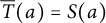 , so
$(H,\cdot ,1,\Delta ,\epsilon ,S)$
 coincides with the transmutation of
$(H,\bullet ,1,\Delta ,\epsilon ,T)$
 . Hence the transmutation of coquasitriangular Hopf algebras gives us examples of Yetter–Drinfeld braces. Theorem 3.10 implies, in particular, that
$\overline {H}$
 lies in
$\mathrm {Hopf}({}^{H^{\bullet }}_{H^{\bullet }}\mathcal {YD})$
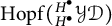 , with action given by
$\rightharpoonup $
 . Observe from duals of [Reference Zhu41, Theorem 4.8 and Corollary 4.9] (with
$f=\mathrm {Id}_{H^{\bullet }}$
 ) that there is a braided monoidal equivalence between
 and
${}^{H^{\bullet }}_{H^{\bullet }}\mathcal {YD}$
 , hence one can also recover an object in
 .
Remark 5.7 We know from Counterexample 2.7 that the following two actions do not form a matched pair:

We may define
$\cdot $
 as in (3.1):

With this product,
$(H,\cdot , 1)$
 is an algebra. But now observe that, since
$\epsilon (a\cdot b)=\mathcal {R}^{-1}(a\otimes b)$
 ,
$\epsilon $
 is not a morphism of algebras with respect to
$\cdot $
 , unless
$\mathcal {R}^{-1}=\epsilon \otimes \epsilon $
 and hence
$\mathcal {R}=\epsilon \otimes \epsilon $
 : in this case, by (coqt.1), H is commutative.
In the case of cocommutative Hopf braces, it is known (see [Reference Angiono, Galindo and Vendramin5, Corollary 2.5]) that the additional operation (3.1) is commutative if and only if the braiding operator
${\sigma (a\otimes b):= (a_1\rightharpoonup b_1)\otimes (a_2\leftharpoonup b_2)}$
 is involutive. An analogous result for Yetter–Drinfed braces may possibly hold, substituting commutativity with braided commutativity in
$^H_H\mathcal {YD}$
 . However, we attempted mimicking the proof of [Reference Angiono, Galindo and Vendramin5, Theorem 2.3] in several straightforward ways, and all of them failed; thus leaving the following problem open:.
Problem 5.8 Let
$(H,\rightharpoonup ,\leftharpoonup )$
 be a matched pair of actions on a Hopf algebra, and let
$\cdot $
 be defined as in (3.1). Is it true that
$\sigma $
 is involutive if and only if
$\cdot $
 is braided-commutative?
Remark 5.9 The well-known FRT construction [Reference Faddeev, Reshetikhin and Takhtajan14] allows one to construct a coquasitriangular bialgebra
$A(c)$
 from a solution
 of the braid equation
$(c\otimes \mathrm {Id})(\mathrm {Id}\otimes c)(c\otimes \mathrm {Id})=(\mathrm {Id}\otimes c)(c\otimes \mathrm {Id})(\mathrm {Id}\otimes c)$
 . The bialgebra
$A(c)$
 is spanned by indeterminates
$t_j^i$
 (see the construction as presented by Kassel [Reference Kassel21]). If we adjoin to
$A(c)$
 inverses
$\bar {t}$
 to the variables, one can canonically extend the relations, the comultiplication and the counit to
$\bar {t}$
 , and define
$St := \bar {t}$
 , obtaining a Hopf algebra
$GL(c)$
 . Suppose now that
$\mathcal {R}$
 extends so that
$GL(c)$
 is coquasitriangular (this happens in many concrete examples, see [Reference Majid30, Section 4.2]). Using the coquasitriangular Hopf algebra
$(GL(c),\mathcal {R})$
 we can obtain a Yetter–Drinfeld brace, where
$\cdot $
 is defined as in (5.6), and S as in and (5.7).
6 Examples
In this section, we apply our results to known examples of coquasitriangular Hopf algebras; namely the Sweedler’s Hopf algebra, the algebras
$E(n)$
 , the Hopf algebra
$\mathrm {SL}_q(2)$
 , and an example in the class of Suzuki algebras. For each example, we describe the corresponding Yetter–Drinfeld brace. Throughout this section, our notation changes from “brace-theoretic”
$(H, \cdot ,\bullet , 1,\Delta , \epsilon , S,T)$
 to “transmutation-theoretic”
$(H,\overline {\cdot }, \cdot , 1,\Delta , \epsilon ,\overline {S},S)$
 , in order to match the way in which the objects in the examples are usually presented.
6.1 The Sweedler’s Hopf algebra
Let us suppose  . The Sweedler’s Hopf algebra
$H_4 = E(1)$
 is the free
 -algebra generated by two elements g and x modulo the relations

where
$1$
 denotes the unit of
$H_4$
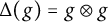
 . It becomes a Hopf algebra with comultiplication, counit and antipode given by
$\Delta (g)=g\otimes g$
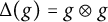 ,
$\Delta (x)=x\otimes 1+g\otimes x$
 ,
$\epsilon (g)=1$
 ,
${\epsilon (x)=0}$
 ,
${S(g)=g}$
 and
$S(x)=xg$
 , respectively. In particular,
$H_4$
 is neither commutative nor cocommutative. We recall that
$H_4$
 has a one-parameter family of cotriangular structures given by

where k is a parameter in  (see [Reference Majid30, Example 2.2.6]). The convolution inverse of
$\mathcal {R}$
 is
$\mathcal {R}^{-1}=\mathcal {R}^{\mathrm {op}}$
 given by the transpose matrix

Given
$\alpha :=a_{1}1+a_{2}g+a_{3}x+a_{4}xg$
 in
$H_4$
 , one has

Hence, given
$\beta :=b_{1}1+b_{2}g+b_{3}x+b_{4}xg$
 in
$H_4$
 , one has

Analogously, for
$\leftharpoonup $
 one has:

Left and right actions for
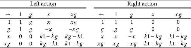
$H_4$
 .

Table 1: Long description
The table is split into two primary sections: Left action and Right action. Each section has a header row and four data rows. The columns for both sections are labeled with the elements 1, g, x, and x g.
Left Action section:
* Row 1 (element 1): The results are 1, g, x, x g.
* Row 2 (element g): The results are 1, g, negative x, minus x g.
* Row 3 (element x): The results are 0, 0, k 1 minus k g, k g minus k 1.
* Row 4 (element x g): The results are 0, 0, k g minus k 1, k 1 minus k g.
Right Action section:
* Row 1 (element 1): The results are 1, 1, 0, 0.
* Row 2 (element g): The results are g, g, 0, 0.
* Row 3 (element x): The results are x, negative x, k 1 minus k g, k 1 minus k g.
* Row 4 (element x g): The results are x g, minus x g, k 1 minus k g, k 1 minus k g.
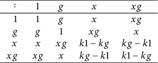
Multiplication table for
$\,\overline {\cdot }\,$
 in
$H_4$
 .
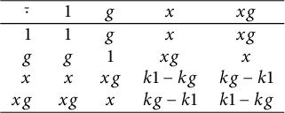
Table 2: Long description
The table defines the operation dot with an overline.
Header Row and Column: The elements are 1, g, x, and x g.
Row 1 (Element 1):
- 1 times 1 is 1.
- 1 times g is g.
- 1 times x is x.
- 1 times x g is x g.
Row 2 (Element g):
- g times 1 is g.
- g times g is 1.
- g times x is x g.
- g times x g is x.
Row 3 (Element x):
- x times 1 is x.
- x times g is x g.
- x times x is k 1 minus k g.
- x times x g is k g minus k 1.
Row 4 (Element x g):
- x g times 1 is x g.
- x g times g is x.
- x g times x is k g minus k 1.
- x g times x g is k 1 minus k g.
The two actions are summarized in Table 1. We denote by
$\,\overline {\cdot }\,$
 the transmuted multiplicative structure on
$H_4$
 , defined according to (5.6). This is explicitly given by

The multiplication
$\,\overline {\cdot }\,$
 is described in Table 2. The algebra
$(H_4, \,\overline {\cdot }\, ,1)$
 is generated by
$g,x$
 modulo the relations
$g \,\overline {\cdot }\, g =1$
 ,
$x\,\overline {\cdot }\, x = k1-kg$
 ,
$x\,\overline {\cdot }\, g= g\,\overline {\cdot }\, x$
 . The new antipode
$\overline {S}$
 is defined by
$\overline {S}(\alpha ):=\alpha _{1}\rightharpoonup S(\alpha _{2})$
 as in (5.7), whence
$\overline {S}(1)=1$
 ,
$\overline {S}(g)=g$
 ,
$\overline {S}(x)= -xg=-x\overline {\cdot }g$
 , and
$\overline {S}(xg) = \overline {S}(x\,\overline {\cdot }\, g)=\overline {S}(g)\,\overline {\cdot }\, \overline {S}(x) = -x$
 . Notice that
$\,\overline {\cdot }\,$
 is braided-commutative and
$\overline {S}$
 is involutive, as we know from Theorem 5.5. Remark 5.2 implies that the braiding
$\sigma _{H_4,H_4}\colon \alpha \otimes \beta \mapsto (\alpha _1\rightharpoonup \beta _1)\otimes (\alpha _2\leftharpoonup \beta _2)$
 is involutive.
Observe that
$\,\overline {\cdot }\,$
 is also commutative, even if
$\sigma ^{\mathcal {YD}}_{H_4,H_4}$
 does not coincide with the flip map
$\tau $
 (for instance, it is easy to see that
$\sigma ^{\mathcal {YD}}_{H_4,H_4}$
 and
$\tau $
 differ on
$x\otimes x$
 ). Notice moreover that
$\,\overline {\cdot }\,$
 is compatible with
$\Delta $
 in the braided sense, but not in the classical sense: indeed
$(x\,\overline {\cdot }\, x)_1\otimes (x\,\overline {\cdot }\, x)_2 = (k1-kg)\otimes (k1-kg) \neq (k1-kg)\otimes 1+2xg\otimes g +1\otimes (k1-kg) = (x_1\,\overline {\cdot }\, x_1)\otimes (x_2\,\overline {\cdot }\, x_2)$
 . In particular, this Yetter–Drinfeld brace is not a Hopf brace.
Remark 6.1 Matched pairs of bialgebras
$(H_4,H_4)$
 on the Sweedler’s Hopf algebra are classified by Bontea [Reference Bontea6, Theorem 2.1]. Other than the matched pairs arising from cotriangular structures, already considered above, there is only one more pair of actions on
$H_4$
 satisfying (mp.1)–(mp.5): this is the pair provided by the trivial actions
$a\otimes b\mapsto \epsilon (a)b$
 ,
$a\otimes b\mapsto a\,\epsilon (b)$
 . Since
$H_4$
 is not commutative, the pair with the trivial actions does not satisfy (⋆), and hence is not a matched pair of actions.
We have, as a byproduct of Remark 6.1, the following result.
Proposition 6.2 The only matched pair of actions
$(H_4,\rightharpoonup ,\leftharpoonup )$
 on the Sweedler’s Hopf algebra
$H_4$
 is the matched pair defined in Table 1.
6.2 The Hopf algebras E(n)
Let us suppose  . A generalization of the Sweedler’s Hopf algebra is provided by the Hopf algebras
$E(n)$
 generated as algebras by
$g, x_i$
 for
$i = 1,\ldots , n$
 , with relations

endowed with the comultiplication
$\Delta (1) = 1\otimes 1$
 ,
$\Delta (g) = g\otimes g$
 ,
$\Delta (x_i) = x_i\otimes 1+ g \otimes x_i$
 , the counit
$\epsilon (g) = 1$
 ,
$\epsilon (x_i) =0$
 , and the antipode
$S(g)=g$
 ,
$S(x_i) = x_i g$
 . The quasitriangular structures on
$E(n)$
 are classified by Panaite and Van Oystaeyen [Reference Panaite and Van Oystaeyen34], and the coquasitriangular structures are obtained by duality (see e.g., Carnovale and Cuadra [Reference Carnovale and Cuadra9, p. 256]):

where
$A=(A_{ij})_{ij}$
 is an
$n\times n$
 matrix with entries in
 . It is easy to see that
$\mathcal {R}_A$
 is cotriangular if and only if A is symmetric. Panaite and Van Oystaeyen [Reference Panaite and Van Oystaeyen34] conjectured that
$R_A$
 is triangular if and only if A is symmetric; which was later proven by Carnovale and Cuadra [Reference Carnovale and Cuadra9, Proposition 2.1].
Assume
$A_{ij} = A_{ji}$
 , thus
$\mathcal {R}^{-1} = \mathcal {R}^{\mathrm {op}}$
 . We define a second multiplicative structure
$\,\overline {\cdot }\,$
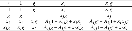
 as in (5.6). This is described in Table 3 (in particular, it is commutative). In terms of generators and relation,
$(E(n), \,\overline {\cdot }\,,1)$
 is the algebra generated by
$g, x_i$
 with relations
$g \,\overline {\cdot }\, g = 1$
 ,
$x_i\,\overline {\cdot }\, x_j + x_j\,\overline {\cdot }\, x_i = 2A_{ij}(1-g)$
 ,
$x_i\,\overline {\cdot }\, g = g\,\overline {\cdot }\, x_i$
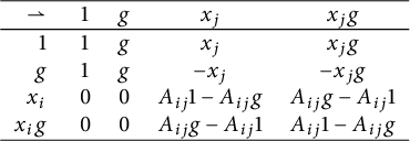
 . The action
$\rightharpoonup $
 is described in Table 4. The antipode
$\overline {S}$
 , defined as in (5.7), acts as follows:
$\overline {S}(1) = 1$
 ,
$\overline {S}(g)=g$
 ,
$\overline {S}(x_i) = -x_i g = -x_i\,\overline {\cdot }\, g$
 .
Multiplication table for
$\,\overline {\cdot }\,$
 in
$E(n)$
 .
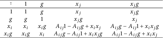
Table 3: Long description
The table consists of a header row and a header column defining the operands, with four rows and four columns of data.
Header Row (Top): 1, g, x sub j, x sub j g.
Header Column (Left): 1, g, x sub i, x sub i g.
Row 1 (Multiplication by 1):
- 1 times 1 yields 1
- 1 times g yields g
- 1 times x sub j yields x sub j
- 1 times x sub j g yields x sub j g
Row 2 (Multiplication by g):
- g times 1 yields g
- g times g yields 1
- g times x sub j yields x sub j g
- g times x sub j g yields x sub j
Row 3 (Multiplication by x sub i):
- x sub i times 1 yields x sub i
- x sub i times g yields x sub i g
- x sub i times x sub j yields A sub i j 1 minus A sub i j g plus x sub i x sub j
- x sub i times x sub j g yields A sub i j g minus A sub i j 1 plus x sub i x sub j g
Row 4 (Multiplication by x sub i g):
- x sub i g times 1 yields x sub i g
- x sub i g times g yields x sub i
- x sub i g times x sub j yields A sub i j g minus A sub i j 1 plus x sub i x sub j g
- x sub i g times x sub j g yields A sub i j 1 minus A sub i j g plus x sub i x sub j
Table for the action
$\rightharpoonup $
 in
$E(n)$
 .
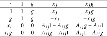
Table 4: Long description
The table consists of five columns and five rows including the header.
Header Row:
- Column 1: right harpoon with barb up operator.
- Column 2: 1.
- Column 3: g.
- Column 4: x sub j.
- Column 5: x sub j g.
Row 2:
- Column 1: 1.
- Column 2: 1.
- Column 3: g.
- Column 4: x sub j.
- Column 5: x sub j g.
Row 3:
- Column 1: g.
- Column 2: 1.
- Column 3: g.
- Column 4: minus x sub j.
- Column 5: minus x sub j g.
Row 4:
- Column 1: x sub i.
- Column 2: 0.
- Column 3: 0.
- Column 4: A sub i j 1 minus A sub i j g.
- Column 5: A sub i j g minus A sub i j 1.
Row 5:
- Column 1: x sub i g.
- Column 2: 0.
- Column 3: 0.
- Column 4: A sub i j g minus A sub i j 1.
- Column 5: A sub i j 1 minus A sub i j g.
6.3 The Hopf algebra SL q (2)
Let  , and consider, following Kassel [Reference Kassel21, Section IV.6], the
 -algebra
$\mathrm {SL}_q(2)$
 generated by
$a,b,c,d$
 modulo the following relations:

This is known to be a Hopf algebra with

and, when
$q\neq 1$
 , it is neither commutative nor cocommutative. The Hopf algebra
$\mathrm {SL}_q(2)$
 is coquasitriangular [Reference Kassel21, Corollary VIII.7.2], with

Notice that
$\mathcal {R}^{-1}=\mathcal {R}^{\mathrm {op}}$
 if and only if
$q^{1/2}=q^{-1/2}$
 , if and only if
$q=1$
 . In this case
$\mathcal {R}=\mathcal {R}^{-1}=\mathcal {R}^{\mathrm {op}}$
 , and the previous matrices are the identities. The explicit form of the iterated
$\Delta $
 is here reported:

We define an additional operation
$\,\overline {\cdot }\,$
 on
$\mathrm {SL}_q(2)$
 as in (5.6). Using the iterated
$\Delta $
 , we compute Table 5 for the multiplication
$\,\overline {\cdot }\,$
 , and Table 6 for the left action
$\rightharpoonup $
 . Hence we have that
$\,\overline {\cdot }\,$
 is commutative if and only if
$q=q^{-1}$
 , i.e., if and only if
$q=\pm 1$
 . In particular, if
$q=-1$
 ,
$\,\overline {\cdot }\,$
 is commutative but
$\mathcal {R}$
 is not cotriangular.
Multiplication table for
$\,\overline {\cdot }\,$
 in
$\mathrm {SL}_q(2)$
 .
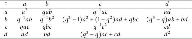
Table 5: Long description
The table consists of 5 columns and 5 rows. The top-left corner cell contains the operator dot-bar. The header row (top) and header column (left) both list the elements a, b, c, and d in that order.
Row 1 (element a):
* a times a yields a-squared.
* a times b yields q a b.
* a times c yields q super negative 1 a c.
* a times d yields a d.
Row 2 (element b):
* b times a yields q super negative 1 a b.
* b times b yields q super negative 1 b-squared.
* b times c yields (q-squared minus 1) a-squared plus (1 minus q-squared) a d plus q b c.
* b times d yields (q-cubed minus q) a b plus b d.
Row 3 (element c):
* c times a yields q a c.
* c times b yields q b c.
* c times c yields q super negative 1 c-squared.
* c times d yields c d.
Row 4 (element d):
* d times a yields a d.
* d times b yields b d.
* d times c yields (q-cubed minus q) a c plus c d.
* d times d yields d-squared.
Table for the action
$\rightharpoonup $
 in
$\mathrm {SL}_q(2)$
 .
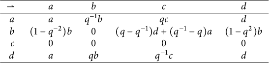
Table 6: Long description
The table consists of a header row and four data rows.
Header Row: The top-left cell contains a right harpoon with barb up symbol. The following columns are headed by the variables a, b, c, and d.
Row 1: Starts with variable a. The results of the action are: a, q super negative 1 b, q c, and d.
Row 2: Starts with variable b. The results of the action are: (1 minus q super negative 2) b, 0, (q minus q super negative 1) d plus (q super negative 1 minus q) a, and (1 minus q squared) b.
Row 3: Starts with variable c. All four result cells in this row contain the value 0.
Row 4: Starts with variable d. The results of the action are: a, q b, q super negative 1 c, and d.
The algebra
$(H,\,\overline {\cdot }\,,1)$
 is generated by
$a,b,c,d$
 modulo the relations


We now define the transmuted antipode
$\overline {S}(x):=x_{1}\rightharpoonup S(x_{2})$
 , as in (5.7). One has

Notice that
$\overline {S}$
 is involutive if and only if
$q = \pm 1$
 . Hence, if
$q=-1$
 ,
$\overline {S}$
 is involutive but
$\mathcal {R}$
 is not cotriangular.
6.4 An example in the class of Suzuki Hopf algebras
Let  be an algebraically closed field of characteristic
 , as in Suzuki [Reference Suzuki38]. The Suzuki Hopf algebra
$A^{\nu ,\lambda }_{1,2}$
 , with parameters
 , is generated by
$a,b,c,d$
 subject to the relations

Let

with
$\mathbf {t}_{ij}$
 denoting the entry on the ith row and jth column. The comultiplication, counit and antipode are respectively given by:

The map

defines a coquasitriangular structure whose convolution inverse is
$\mathcal {R}^{-1}_{(\alpha ,\beta )} = \mathcal {R}_{(\alpha ^{-1},\beta ^{-1})}$
 (see [Reference Suzuki38, proof of Proposition 2.1]), which is cotriangular if
$(\alpha ,\beta ) = (-1,-1)$
 or
$(\alpha ,\beta )=(1,1)$
 , and
$(\nu ,\lambda ) = (1,1)$
 (see [Reference Suzuki38, Proposition 3.10]).
We define an algebra operation
$\,\overline {\cdot }\,$
 as in (5.6), whose multiplication table is reported in Table 7. In particular,
$\,\overline {\cdot }\,$
 is commutative. The algebra
$(H,\,\overline {\cdot }\,,1)$
 is generated by
$a,b,c,d$
 modulo the relations

The action
$\rightharpoonup $
 is reported in Table 8. The corresponding antipode
$\overline {S}$
 , defined as in (5.7), is identified by
$\overline {S} (a) = \alpha ^2\beta ^2 d^3$
 ,
$\overline {S}(b) = \alpha ^3\beta b^3$
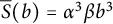 ,
$\overline {S}(c) = \alpha ^3\beta c^3$
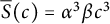 ,
$\overline {S}(d) = \alpha ^2\beta ^2 a^3$
 .
Multiplication table for
$\,\overline {\cdot }\,$
 in
$A_{1,2}^{\nu ,\lambda }$
 .
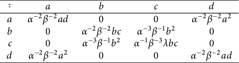
Table 7: Long description
The table defines the multiplication of elements a, b, c, and d.
Header Row: The columns are labeled a, b, c, and d.
Row 1 (a):
- a times a is alpha super negative 2 beta super negative 2 a d.
- a times b is 0.
- a times c is 0.
- a times d is alpha super negative 2 beta super negative 2 a-squared.
Row 2 (b):
- b times a is 0.
- b times b is alpha super negative 2 beta super negative 2 b c.
- b times c is alpha super negative 3 beta super negative 1 b-squared.
- b times d is 0.
Row 3 (c):
- c times a is 0.
- c times b is alpha super negative 3 beta super negative 1 b-squared.
- c times c is alpha super negative 1 beta super negative 3 lambda b c.
- c times d is 0.
Row 4 (d):
- d times a is alpha super negative 2 beta super negative 2 a-squared.
- d times b is 0.
- d times c is 0.
- d times d is alpha super negative 2 beta super negative 2 a d.
Table for the action
$\rightharpoonup $
 in
$A^{\nu ,\lambda }_{1,2}$
 .
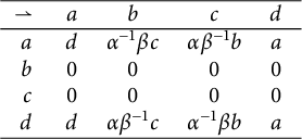
Table 8: Long description
The table consists of five columns and five rows.
Header Row: The first cell contains a right harpoon with barb up symbol. The following headers are a, b, c, and d.
Row 1: The row header is a. The corresponding values are d, alpha super negative 1 beta c, alpha beta super negative 1 b, and a.
Row 2: The row header is b. All corresponding values in this row are 0.
Row 3: The row header is c. All corresponding values in this row are 0.
Row 4: The row header is d. The corresponding values are d, alpha beta super negative 1 c, alpha super negative 1 beta b, and a.
We know by Theorem 5.5 that the additional operation (3.1) is braided commutative if
$\mathcal {R}$
 is cotriangular. In all the previous examples, when
$\mathcal {R}$
 is cotriangular (3.1) is also commutative. We could neither prove nor disprove that this is true in general, and thus the following problem is open.
Problem 6.3 Let
$(H,\mathcal {R})$
 be a cotriangular Hopf algebra. Is it true that the additional operation (5.6) is commutative?
Notice that the converse is false (see the example
$SL_q(2)$
 with
$q = -1$
 ).
Acknowledgements
The authors would like to thank A. Ardizzoni for meaningful suggestions throughout all phases of this work, and L. Vendramin and T. Weber for valuable comments. This paper was written while the authors were members of the “National Group for Algebraic and Geometric Structures and their Applications” (GNSAGA-INdAM).