2 Formulation

We restrict our attention to the steady two-dimensional flow equations that model equilibrium fluid dynamics in the limit of vanishing viscosity and heat conductivity, namely the steady two-dimensional Euler equations

(2.1) $$\begin{eqnarray}\unicode[STIX]{x2202}_{x}F_{x}(q)+\unicode[STIX]{x2202}_{y}F_{y}(q)=0,\end{eqnarray}$$

where

(2.2) $$\begin{eqnarray}q=(\unicode[STIX]{x1D70C},\unicode[STIX]{x1D70C}u_{x},\unicode[STIX]{x1D70C}u_{y},\unicode[STIX]{x1D70C}e+\unicode[STIX]{x1D70C}u^{2}/2)\end{eqnarray}$$

is the vector of conservative variables, in which $\unicode[STIX]{x1D70C}$ is the density, $u_{x}$ , $u_{y}$ and $u$ are the velocity $x$ -component, $y$ -component and magnitude, respectively, and $e$ is the specific internal energy. The fluxes $F_{x}$ and $F_{y}$ are given by

(2.3) $$\begin{eqnarray}\displaystyle & \displaystyle F_{x}(q)=(\unicode[STIX]{x1D70C}u_{x},\unicode[STIX]{x1D70C}u_{x}^{2}+P,\unicode[STIX]{x1D70C}u_{x}u_{y},\unicode[STIX]{x1D70C}h^{t}u_{x}), & \displaystyle\end{eqnarray}$$

(2.4) $$\begin{eqnarray}\displaystyle & \displaystyle F_{y}(q)=(\unicode[STIX]{x1D70C}u_{y},\unicode[STIX]{x1D70C}u_{x}u_{y},\unicode[STIX]{x1D70C}u_{y}^{2}+P,\unicode[STIX]{x1D70C}h^{t}u_{y}), & \displaystyle\end{eqnarray}$$

where $h^{t}=e+P/\unicode[STIX]{x1D70C}+u^{2}/2$ is the specific total enthalpy per unit mass.

The steady two-dimensional Euler equations are classified as elliptic, parabolic or hyperbolic depending on the value of the flow Mach number $M$ ,

(2.5) $$\begin{eqnarray}M=u/c,\end{eqnarray}$$

see, e.g. Godlewski & Raviart (Reference Godlewski and Raviart2013). System (2.1) is of the elliptic type if $M<1$ and of the parabolic type if $M=1$ . If $M>1$ , system (2.1) is hyperbolic in every direction (i.e. the time-like direction) that is not perpendicular to characteristic lines (Dafermos Reference Dafermos2010).

In a Cartesian $x$ – $y$ coordinate system, we consider, with reference to the ramp problem, a solid boundary described by the equations

(2.6) $$\begin{eqnarray}\displaystyle & \displaystyle y=0,\quad x\leqslant 0, & \displaystyle\end{eqnarray}$$

(2.7) $$\begin{eqnarray}\displaystyle & \displaystyle y=(\tan \unicode[STIX]{x1D717}_{r})x,\quad x>0, & \displaystyle\end{eqnarray}$$

where $\unicode[STIX]{x1D717}_{r}$ is the ramp angle. The corner of the ramp is thus located at $x=0$ , $y=0$ . Along the solid wall, a slip boundary condition is enforced. A uniform flow state is prescribed at infinity upstream $x=-\infty$ , which is aligned with the wall ( $u_{y}=0$ ) and supersonic.

In this study, self-similar solutions of the steady supersonic ramp problem are examined. These are functions of the form $q(x,y)=w(y/x)$ that satisfy the integral form of the conservation law associated with (2.1) in the domain (circular sector) delimited by the solid wall, along with the boundary conditions imposed on the wall itself and at upstream infinity. On physical grounds, we shall also limit ourselves to considering self-similar solutions that are piecewise $C^{1}$ . Introducing $\unicode[STIX]{x1D709}=y/x$ , this means that $w(\unicode[STIX]{x1D709})$ is continuously differentiable except for a finite number of points at which $w$ has a jump discontinuity or is continuous but not differentiable. As a consequence, we examine solutions that are constant along rays emanating from the corner of the ramp; in the solution flow field, a finite number of rays, carrying jump discontinuities in $w$ or its gradient, separate circular sectors where $w$ is continuously differentiable. In the following, the building blocks for the construction of self-similar solutions of the steady supersonic ramp problem are described. These are the continuously differentiable simple waves, the discontinuous waves (shocks and contacts) and the composite waves, which are combination of the previous ones.

2.1 Simple waves

The flow pattern corresponding to a non-trivial, continuously differentiable function $w(\unicode[STIX]{x1D709})$ is called a centred simple wave and in the physical plane it takes the form of a fan, commonly denoted the Prandtl–Meyer fan, converging at a single point. At points where $w(\unicode[STIX]{x1D709})$ is continuous and differentiable, equation (2.1) is equivalent to the generalized eigenvalue problem

(2.8) $$\begin{eqnarray}(A_{y}(w(\unicode[STIX]{x1D709}))-\unicode[STIX]{x1D709}A_{x}(w(\unicode[STIX]{x1D709})))w^{\prime }(\unicode[STIX]{x1D709})=0,\end{eqnarray}$$

where $A_{x}(q)=D_{q}F_{x}(q)$ and $A_{y}(q)=D_{q}F_{y}(q)$ are the Jacobians of the fluxes. It follows that either $w^{\prime }(\unicode[STIX]{x1D709})=0$ or

(2.9) $$\begin{eqnarray}\unicode[STIX]{x1D709}=\unicode[STIX]{x1D706}_{k}(w(\unicode[STIX]{x1D709})),\quad \text{for some }k\in \{1,\ldots ,4\}\end{eqnarray}$$

and

(2.10) $$\begin{eqnarray}w^{\prime }(\unicode[STIX]{x1D709})=r_{k}(w(\unicode[STIX]{x1D709}))/\unicode[STIX]{x1D6FC}_{k}(w(\unicode[STIX]{x1D709})),\quad \text{for some }k\in \{1,\ldots ,4\},\end{eqnarray}$$

where $\unicode[STIX]{x1D706}_{k}$ and $r_{k}$ denote the $k$ th eigenvalue and right eigenvector, respectively, in the generalized eigenvalue problem (2.8) and $\unicode[STIX]{x1D6FC}_{k}=D_{q}\unicode[STIX]{x1D706}_{k}(q)\cdot r_{k}(q)$ is the $k$ th nonlinearity factor (see appendix A). Note also that the ray marking the transition between a simple-wave region and a uniform flow region is a point of jump discontinuity for $w^{\prime }(\unicode[STIX]{x1D709})$ .

Since $\unicode[STIX]{x1D709}=x/y$ is a real number, relation (2.9) implies that the eigenvalue $\unicode[STIX]{x1D706}_{k}$ is also real. It is well known (see, e.g. Thompson Reference Thompson1988) that the characteristic equation of the eigenvalue problem (2.8) always gives a real root $\unicode[STIX]{x1D706}=\tan \unicode[STIX]{x1D717}$ of multiplicity two, where $\unicode[STIX]{x1D717}=\tan ^{-1}(u_{y}/u_{x})$ is the angle formed by the particle path with the $x$ -axis (positive if counter-clockwise), whereas the remaining roots are real if and only if the flow is supersonic ( $M>1$ ). For supersonic flow, the eigenvalues of the steady planar Euler equations can be written as

(2.11a-c ) $$\begin{eqnarray}\unicode[STIX]{x1D706}_{1}=\tan (\unicode[STIX]{x1D717}-\unicode[STIX]{x1D707}),\quad \unicode[STIX]{x1D706}_{2,3}=\tan \unicode[STIX]{x1D717},\quad \unicode[STIX]{x1D706}_{4}=\tan (\unicode[STIX]{x1D717}+\unicode[STIX]{x1D707}),\end{eqnarray}$$

in which the angle $\unicode[STIX]{x1D707}=\sin ^{-1}(1/M)$ is called the Mach angle. The characteristic curves, having slope $\text{d}y/\text{d}x=\unicode[STIX]{x1D706}_{k}$ in the physical $x$ – $y$ plane, are thus the particle paths and the curves that locally form an angle $\pm \unicode[STIX]{x1D707}$ with the particle paths. Because of this, the characteristics of the 1-field and 4-field (the $k$ -field is the characteristic field associated with $\unicode[STIX]{x1D706}_{k}$ and $r_{k}$ ) are also referred to as right-running and left-running acoustic waves, respectively. Equation (2.9) implies that the rays in a centred simple wave correspond to characteristic lines.

Relation (2.10) asserts that the states within a centred simple wave all lie along an integral curve of $r_{k}(q)$ . However, in order that $w^{\prime }(\unicode[STIX]{x1D709})$ stays finite, the nonlinearity factor appearing in (2.10) must not be zero. With a proper scaling of the eigenvectors, the nonlinearity factors read (appendix A)

(2.12a,b ) $$\begin{eqnarray}\unicode[STIX]{x1D6FC}_{1,4}=\unicode[STIX]{x1D6E4},\quad \unicode[STIX]{x1D6FC}_{2,3}=0,\end{eqnarray}$$

thus showing, together with relation (2.10), that continuously differentiable waves are not possible in the 2-field and 3-field (which are linearly degenerate and give rise to contact discontinuities, see § 2.2) and in the 1-field and 4-field at degenerate points $\unicode[STIX]{x1D6E4}=0$ . In other words, centred simple waves can only take place in the acoustic wave families (1-field or 4-field) if $\unicode[STIX]{x1D6E4}\neq 0$ .

For each characteristic field of an $n$ -dimensional system of conservation laws (in our case $n=4$ ) is defined a set of $n-1$ Riemann invariants (Dafermos Reference Dafermos2010). A Riemann invariant of the $k$ th field is a scalar-valued function that is constant along the integral curve of $r_{k}(q)$ . The Riemann invariants of the 1-field and 4-field are the triplets

(2.13) $$\begin{eqnarray}\left\{\begin{array}{@{}l@{}}s,h^{t},\unicode[STIX]{x1D717}-\unicode[STIX]{x1D708}\quad \text{(1-field)},\quad \\ s,h^{t},\unicode[STIX]{x1D717}+\unicode[STIX]{x1D708}\quad \text{(4-field)},\quad \end{array}\right.\end{eqnarray}$$

where

(2.14) $$\begin{eqnarray}\unicode[STIX]{x1D708}=\unicode[STIX]{x1D708}_{0}+\int _{u_{0}}^{u}\sqrt{M^{2}-1}\,\frac{\text{d}u}{u}=\unicode[STIX]{x1D708}_{0}-\int _{P_{0}}^{P}\frac{\sqrt{M^{2}-1}}{\unicode[STIX]{x1D70C}u^{2}}\,\text{d}P\end{eqnarray}$$

is the Prandtl–Meyer function, in which subscript 0 refers to a reference state (in fluids exhibiting $\unicode[STIX]{x1D6E4}<1$ , the above forms of the Prandtl–Meyer function are valid at all velocities and pressures, contrary to the more common form parametrized using the Mach number, see Cramer & Crickenberger Reference Cramer and Crickenberger1992). Therefore, the flow field within a centred simple wave has constant entropy and total enthalpy. By examining the eigenvectors $r_{1}$ and $r_{4}$ (see appendix A), it is readily seen that $P^{\prime }(\unicode[STIX]{x1D709})\gtrless 0$ , $u^{\prime }(\unicode[STIX]{x1D709})\lessgtr 0$ and $\unicode[STIX]{x1D717}^{\prime }(\unicode[STIX]{x1D709})\gtrless 0$ if $\unicode[STIX]{x1D6E4}\gtrless 0$ within left-running simple waves, while $P^{\prime }(\unicode[STIX]{x1D709})\lessgtr 0$ , $u^{\prime }(\unicode[STIX]{x1D709})\gtrless 0$ and $\unicode[STIX]{x1D717}^{\prime }(\unicode[STIX]{x1D709})\gtrless 0$ if $\unicode[STIX]{x1D6E4}\gtrless 0$ in right-running simple waves.

2.2 Shock waves and contact discontinuities

The turning of a supersonic stream can also be accomplished by means of discontinuous waves. If $w$ has a jump discontinuity along the ray $\unicode[STIX]{x1D709}$ , the balance laws of mass, momentum and energy assume the form

(2.15) $$\begin{eqnarray}[F_{y}-\unicode[STIX]{x1D709}F_{x}]=0,\end{eqnarray}$$

where $[\cdot ]$ denotes the jump across the discontinuity. Equations (2.15) are the well-known set of Rankine–Hugoniot relations (see, e.g. Thompson Reference Thompson1988), which can be conveniently recast as

(2.16) $$\begin{eqnarray}\displaystyle & \displaystyle [\unicode[STIX]{x1D70C}u_{n}]=0, & \displaystyle\end{eqnarray}$$

(2.17) $$\begin{eqnarray}\displaystyle & \displaystyle [P+\unicode[STIX]{x1D70C}u_{n}^{2}]=0, & \displaystyle\end{eqnarray}$$

(2.18) $$\begin{eqnarray}\displaystyle & \displaystyle [\unicode[STIX]{x1D70C}u_{n}u_{t}]=0, & \displaystyle\end{eqnarray}$$

(2.19) $$\begin{eqnarray}\displaystyle & \displaystyle [\unicode[STIX]{x1D70C}u_{n}h^{t}]=0, & \displaystyle\end{eqnarray}$$

where $u_{n}$ and $u_{t}$ are the normal and tangential velocity components, with respect to the shock front. System (2.16)–(2.19) includes both contact discontinuities and shock waves, which are distinguished according to the value of the mass flux $m=\unicode[STIX]{x1D70C}u_{n}$ across the discontinuity front. For contact discontinuities $m=0$ , while for shock waves $m\neq 0$ .

The states that can be connected by means of contact discontinuities lie on the integral curves of $r_{2}(q)$ and $r_{3}(q)$ , see Godlewski & Raviart (Reference Godlewski and Raviart2013). The corresponding Riemann invariants are

(2.20) $$\begin{eqnarray}\left\{\begin{array}{@{}l@{}}P,\unicode[STIX]{x1D717},s\quad \text{(2-field)},\quad \\ P,\unicode[STIX]{x1D717},u\quad \text{(3-field)},\quad \end{array}\right.\end{eqnarray}$$

thus indicating that the discontinuous waves of the 2-field are vorticity waves (or slip lines, i.e. jumps in the velocity magnitude at the same pressure, entropy and flow direction) and those of the 3-field are entropy waves (i.e. entropy jumps at constant pressure and velocity).

Shock waves are discontinuities in the acoustic wave families (1-field and 4-field) and thanks to the conservation of the tangential velocity (2.18) they can be represented as normal shocks to which a uniform velocity field, parallel to the shock front, is superposed. It is easily checked that if the normal velocity decreases when the shock front is crossed (from the mass and normal momentum relations, the shock is compressive), the shock wave deviates the flow towards the front itself; the opposite occurs if the normal velocity increases (rarefaction shock). This means that $[\unicode[STIX]{x1D717}]\gtrless 0$ if $[P]\gtrless 0$ for left-running shock waves (4-field) and $[\unicode[STIX]{x1D717}]\lessgtr 0$ if $[P]\gtrless 0$ for right-running shocks (1-field). In addition, from (2.19) with $\unicode[STIX]{x1D70C}u_{n}\neq 0$ , it follows the total enthalpy is conserved across the shock. The jump conditions can be combined into the well-known Hugoniot relation

(2.21) $$\begin{eqnarray}[h]-{\textstyle \frac{1}{2}}[P](v_{-}+v_{+})=0,\end{eqnarray}$$

where subscripts ‘ $-$ ’ and ‘ $+$ ’ denote the pre-shock and post-shock state, respectively. The Hugoniot relation determines the set (Hugoniot locus) of the thermodynamic states that can be connected by means of a shock wave. In the $P$ – $v$ plane, the Hugoniot locus is commonly referred to as the shock adiabat.

The Rankine–Hugoniot relations must be complemented with suitable admissibility criteria in order to rule out unphysical solutions. The second law of thermodynamics requires that the entropy does not decrease across the shock, namely

(2.22) $$\begin{eqnarray}s_{+}\geqslant s_{-}.\end{eqnarray}$$

For the shock front to be stable against normal perturbations, the speed ordering relation

(2.23) $$\begin{eqnarray}M_{n+}\leqslant 1\leqslant M_{n-},\end{eqnarray}$$

where $M_{n}=u_{n}/c$ is the normal flow Mach number, must be satisfied (Landau & Lifshitz Reference Landau and Lifshitz1987). Conditions (2.22) and (2.23) have a useful geometrical interpretation in the $P$ – $v$ plane (see Thompson & Lambrakis Reference Thompson and Lambrakis1973; Cramer Reference Cramer1989b ; Kluwick Reference Kluwick2001). For an entropy increasing shock, the area between $v_{-}$ and $v_{+}$ under the shock adiabat must be larger than that under the Rayleigh line, the straight line connecting the pre-shock and post-shock states (from equations (2.16)–(2.17), the slope of the Rayleigh line is $[P]/[v]=-m^{2}$ ). The speed ordering relation results in the following condition on the slopes of the shock adiabat and Rayleigh line:

(2.24) $$\begin{eqnarray}\left.\frac{\text{d}P}{\text{d}v}\right|_{+}\leqslant \frac{[P]}{[v]}\leqslant \left.\frac{\text{d}P}{\text{d}v}\right|_{-},\end{eqnarray}$$

where the derivative is taken along the shock adiabat centred on ( $P_{-}$ , $v_{-}$ ). A further criterion is that the Rayleigh line must not cut the shock adiabat at interior points; this amounts to require the existence of the one-dimensional thermoviscous profile associated with the normal flow (Cramer Reference Cramer1989b ). Some consequences of these admissibility criteria are as follows. For convex shock adiabats as in classical gas dynamics, the above requirements are simultaneously satisfied if and only if the shock is pressure increasing. If the shock adiabat is non-convex, there may appear branches where only rarefaction shocks are admissible (for example, in the region where the shock adiabat is concave) or where one or more of the above conditions fail and therefore no shock wave is admissible.

In multi-dimensional flows, an additional requirement is that the shock front is not unstable to transverse perturbations. This condition, introduced by D’yakov (Reference D’yakov1954) and Erpenbeck (Reference Erpenbeck1962), reads

(2.25) $$\begin{eqnarray}-1\leqslant -\frac{[P]}{[v]}\left(\left.\frac{\text{d}P}{\text{d}v}\right|_{+}\right)^{-1}\leqslant 1+2M_{n+}.\end{eqnarray}$$

Assuming $\text{d}P/\text{d}v|_{+}<0$ , which is the typical behaviour for most real fluids (Landau & Lifshitz Reference Landau and Lifshitz1987) and it is also observed here throughout, condition (2.25) is satisfied if the speed ordering relation holds. Additional comments concerning the neutral stability to transverse perturbations are provided at the end of § 5.

3 Solution of the ramp problem and wave curves

With reference to the ramp problem, we now investigate the wave configurations that can possibly deliver the turning of a uniform supersonic stream in a steady flow. Across entropy and shear waves there is neither mass flux nor deviation of the particle paths (cf. (2.20)), therefore the uniform supersonic flow can be turned only across acoustic or shock waves. We immediately note that the presence of both left-running and right-running waves emanating from the ramp corner is not compatible with the boundary conditions imposed by the solid boundary. Thus, if the flow domain is above the solid boundary (e.g. $y>0$ for the uniform supersonic stream), only a left-running wave can deliver the deflection of the upstream flow and it is at the same time compatible with the condition of flow uniformity at upstream infinity. On the contrary, a right-running wave is required if the flow domain is below the solid boundary.

Downstream of these wave patterns, a slip line bringing the flow to rest can always be added without changing the overall deflection (several contact waves can be added further downstream). Because we are ultimately interested in describing the structure of the waves that can possibly deliver the turning of the uniform supersonic stream, henceforth we conveniently assume that the angle $\unicode[STIX]{x1D717}_{r}$ appearing in (2.7) coincides with the flow deviation across waves of the acoustic fields i.e. oblique waves. That is, the following treatment is valid if one interprets the ramp angle as the turning angle of the uniform supersonic flow (in the absence of downstream contact waves, this is exactly the angle of the solid boundary).

In terms of self-similar wave patterns, the two-dimensional steady supersonic flow involves several analogies with the one-dimensional unsteady case. As is well known (see, e.g. Godlewski & Raviart Reference Godlewski and Raviart2013), the unsteady one-dimensional Euler equations possess two acoustic characteristic fields corresponding to left-facing and right-facing waves (propagating with speed $u\mp c$ , respectively), with a linearly degenerate field corresponding to contact discontinuities (propagating with speed $u$ ) in between. In both two-dimensional steady supersonic flows and one-dimensional unsteady flows, the acoustic fields have a similar structure thanks to the following facts. Smooth wave patterns occur, in both cases, in the form of centred fans of acoustic waves. The nonlinearity factor of the acoustic fields, in both cases, are proportional to $\unicode[STIX]{x1D6E4}$ , which means that the breakdown of simple waves coincides with the condition $\unicode[STIX]{x1D6E4}=0$ both in two-dimensional steady supersonic flows and in one-dimensional unsteady flows (in turn, this implies that the mechanism of formation of composite waves is the same). Moreover, oblique shocks in two dimensions satisfy the one-dimensional Rankine–Hugoniot relations in the direction normal to the shock front. Thus, steady Prandtl–Meyer fans and oblique shocks are the counterparts of unsteady wave fans and normal shocks, respectively. The correspondence between the elementary wave patterns makes it possible to extend many of the concepts developed for the one-dimensional unsteady case to the steady two-dimensional one. On the other hand, two differences between these frameworks are as follows. In two-dimensional steady flows, self-similar waves can separate hyperbolic and elliptic regions of the flow fields. This change can possibly occur across strong oblique shocks, which drive the Mach number below unity. Secondly, in two-dimensional steady flows, there exists a maximum pressure jump across shock waves, due to the fact that the total enthalpy is constant (cf. (2.13) and (2.19)) along streamlines. In contrast, in one-dimensional unsteady flows, any value of the pressure jump can be attained depending on the shock speed.

To formalize the similarity between one-dimensional unsteady flows and two-dimensional steady flows, we introduce here the idea of wave curve for steady two-dimensional flows. In one-dimensional unsteady flows, the wave curve represents the set of states connected to a given initial state by a self-similar wave of the left-facing or right-facing field (Menikoff & Plohr Reference Menikoff and Plohr1989). In two-dimensional steady flows, the wave curve consists of all the states connected to a given supersonic state by means of a steady self-similar planar wave of the left-running or right-running field. Thus, the wave curve is made of branches corresponding to centred simple waves, shock waves and composite waves. In the context of the supersonic ramp problem, the wave curve computed from the state associated with the uniform supersonic stream embeds all the self-similar waves that can possibly deliver the deflection imposed by the ramp (in the above sense).

Similarly to the one-dimensional case, the construction of wave curves can be simplified by first considering the projection onto the thermodynamic variables; the kinematic quantities are retrieved afterwards. This two-step procedure is the topic of the next sections. Three important observations set the ground for the following treatment:

1. (i) the projection of a Prandtl–Meyer fan connected to an upstream state A, onto the thermodynamic variables, is a branch of the isentrope passing through the upstream thermodynamic state (cf. the Riemann invariants (2.13)). Given, e.g. the downstream pressure $P_{B}$ , all the thermodynamic quantities downstream of the fan are readily determined. The kinematic quantities (e.g. $u_{B}$ and $\unicode[STIX]{x1D717}_{B}$ ) are computed by imposing the conservation of the total enthalpy $h^{t}$ and of the Riemann invariant $\unicode[STIX]{x1D703}\mp \unicode[STIX]{x1D708}$ of opposite sign;

2. (ii) shock waves connected to state A project, in the thermodynamic plane, onto a branch of the Hugoniot locus passing through the upstream thermodynamic state (cf. equation (2.21)). Given, e.g. the downstream pressure, the downstream density is computed from (2.21) and, from those, each downstream thermodynamic quantity and the mass flux $m=(-[P]/[v])^{1/2}$ . The shock angle $\unicode[STIX]{x1D6FD}_{s}$ and flow deflection angle $\unicode[STIX]{x1D717}_{B}$ (with respect to the upstream flow direction) are computed from $m=\unicode[STIX]{x1D70C}_{A}u_{A}\sin \unicode[STIX]{x1D6FD}_{s}$ and $\unicode[STIX]{x1D70C}_{A}\tan \unicode[STIX]{x1D6FD}_{s}=\unicode[STIX]{x1D70C}_{B}\tan (\unicode[STIX]{x1D6FD}_{s}-\unicode[STIX]{x1D717}_{B})$ , respectively;

3. (iii) Prandtl–Meyer fans cannot be continued at states of linear degeneracy $\unicode[STIX]{x1D6E4}=0$ , because there the characteristic lines fold. If a further pressure variation is imposed, this is accomplished by means of a composite wave in which the fan terminates in a pre-sonic oblique shock (Menikoff & Plohr Reference Menikoff and Plohr1989). The shock-wave branch of the wave curve cannot be continued at entropy extrema, whereby the Rayleigh line is tangent to the shock adiabat, because a further variation in the post-shock pressure would lead to violation of the speed ordering relation (2.23). The wave curve beyond an entropy extremum in the Hugoniot locus is continued as a composite shock/fan wave. By collecting the states downstream of the composite wave, a composite locus is obtained (see also Kluwick Reference Kluwick2001).

4 Wave curves in the thermodynamic plane

Let us consider the structure of the wave-curve projection onto the thermodynamic variables, say the $P$ – $v$ plane. Remarks (i) and (ii) in the previous section imply that, for a given upstream state, the projected wave curve is a subset of the one-dimensional unsteady counterpart. The kinematic state of the upstream flow, through the value of the total enthalpy which remains constant throughout the flow field and limits the maximum pressure jump across oblique shocks, determines endpoints of the wave curve. This suggests that one can use the well-established results for the one-dimensional unsteady case (replacing, of course, unsteady wave fans with Prandtl–Meyer waves and unsteady normal shocks with steady oblique shocks) to determine the underlying structure of the wave curve in the thermodynamic plane, namely the extended (i.e. drawn up to vacuum and infinite pressure) wave curve. The upstream kinematic state is then taken into account (in the following section) to determine endpoints of the waves curves.

In order to illustrate the different types of wave curves in a typical BZT fluid, the polytropic van der Waals model (namely with constant isochoric specific heat) of a molecularly complex fluid is considered. Several previous studies have proved the soundness of the adoption of this simple model for qualitative analyses, owing to the fact that the negative- $\unicode[STIX]{x1D6E4}$ region is well captured (Thompson & Lambrakis Reference Thompson and Lambrakis1973; Kluwick Reference Kluwick2001; Guardone, Vigevano & Argrow Reference Guardone, Vigevano and Argrow2004; Guardone & Argrow Reference Guardone and Argrow2005). The fluid selected for this purpose is siloxane MDM (octamethyltrisiloxane, $\text{C}_{8}\text{H}_{24}\text{O}_{2}\text{Si}_{3}$ ) with $c_{v}/R=57.69$ , where $c_{v}$ is the isochoric heat capacity and $R$ is the gas constant.

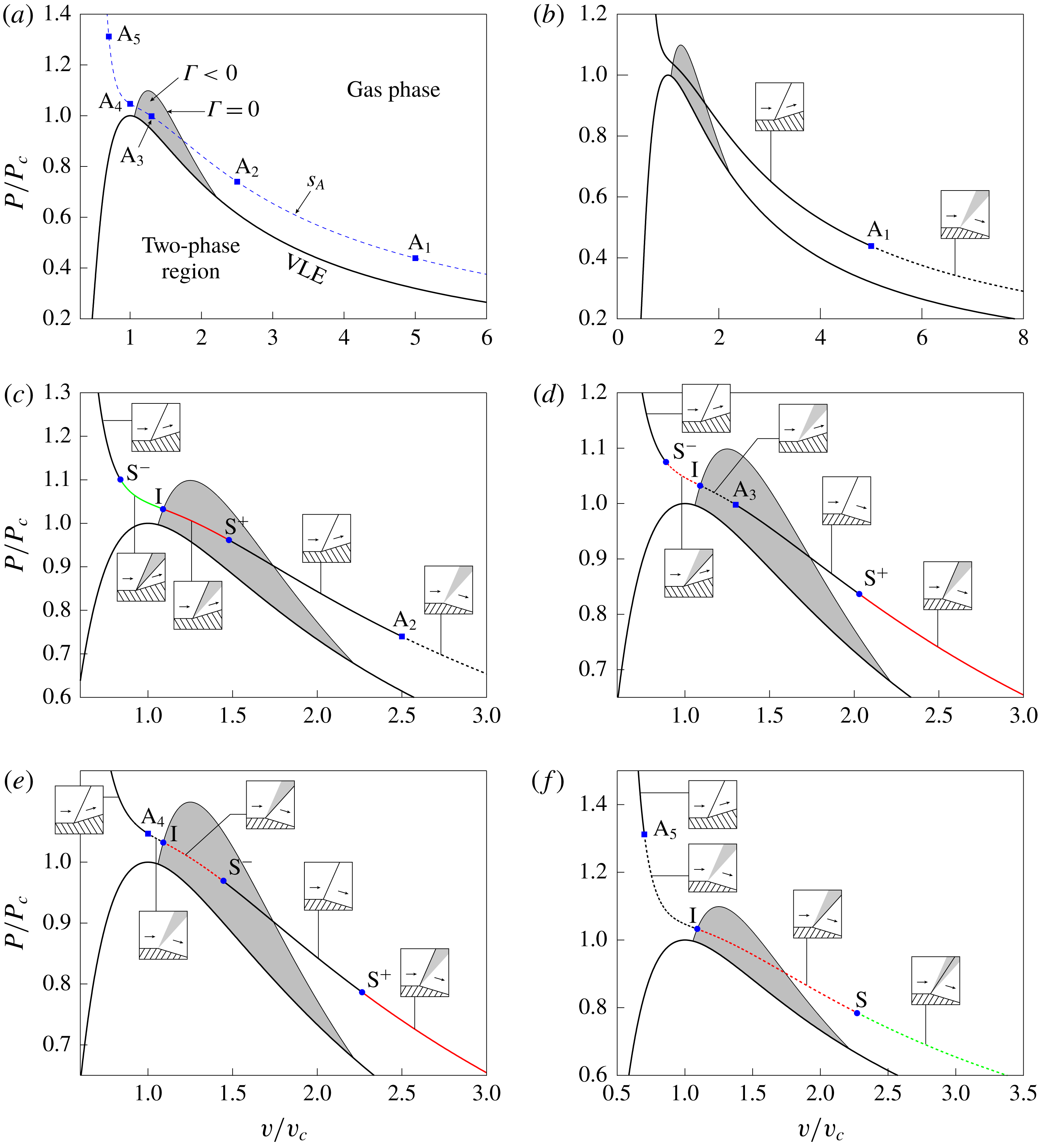
Five thermodynamic states are chosen along the same isentrope $s_{A}$ crossing the negative- $\unicode[STIX]{x1D6E4}$ region while remaining in the single phase, as shown in figure 1(a). The corresponding extended wave curves in the $P$ – $v$ plane are shown in figure 1(b–f). These are now detailed.

Figure 1.

Extended wave curves in the pressure–specific volume diagram (subscript $c$ indicates critical-point quantities) computed from the polytropic van der Waals model of fluid MDM. (a) The selected upstream states, chosen along an isentrope crossing the negative- $\unicode[STIX]{x1D6E4}$ region (shaded area). (b–f) Extended wave curve for each upstream state. Wave configurations: —— (black) shock, —— (red) shock/fan, —— (green) shock/fan/shock, – – – (black) fan, – – – (red) fan/shock, – – – (green) fan/shock/fan. Point $\text{S}^{+}$ : downstream state of post-sonic oblique shock; point $\text{S}^{-}$ : downstream state of pre-sonic oblique shock; point S: downstream state of double-sonic oblique shock; point I: intersection between the local isentrope and the $\unicode[STIX]{x1D6E4}=0$ locus. Attached to each branch is a qualitative sketch of the (left-running) wave configuration in the physical plane, where thick lines denote oblique shocks and shaded areas denote wave fans.

Case 1 – figure 1(b). Thermodynamic state $\text{A}_{1}$ is located on the right-hand side of the negative- $\unicode[STIX]{x1D6E4}$ region. Thus, the rarefaction branch of the extended wave curve through $\text{A}_{1}$ is the isentrope containing $\text{A}_{1}$ , associated with elementary Prandtl–Meyer waves connected to $\text{A}_{1}$ . On the other hand, the compressive branch of the wave curve coincides with the shock adiabat centred on $\text{A}_{1}$ , associated with oblique shock waves. Note that, despite the shock adiabat crossing the negative- $\unicode[STIX]{x1D6E4}$ region and the fact that it is non-convex, no entropy extrema occur. Graphically, this means the Rayleigh line (straight line connecting the pre-shock and post-shock states) is never tangent to the shock adiabat at the post-shock state. The same wave-curve configuration (compression shock and rarefaction fan branches) is observed whenever the isentrope passing through the upstream state is convex (see, e.g. Kluwick Reference Kluwick2001).

Case 2 – figure 1(c). Similarly to case 1, thermodynamic state $\text{A}_{2}$ is on the right-hand side of the negative- $\unicode[STIX]{x1D6E4}$ region. The rarefaction branch of the wave curve, therefore, is as in the previous case. On the contrary, the compression branch is significantly different. The wave curve is still, for moderate pressure rises, the locus of the oblique shocks connected to $\text{A}_{2}$ . In contrast to case 1, however, there exists a downstream pressure (point $\text{S}^{+}$ ) for which the entropy along the shock adiabat reaches a local maximum (i.e. the Rayleigh line is tangent to the shock adiabat at $\text{S}^{+}$ ); shock $\text{A}_{2}$ – $\text{S}^{+}$ is indeed a post-sonic compression shock. As mentioned in § 3, the wave curve is continued along the isentrope passing through $\text{S}^{+}$ , for a composite oblique shock/Prandtl–Meyer fan combination. The fan in the composite wave cannot be continued beyond point I, where the isentrope through $\text{S}^{+}$ intersects the $\unicode[STIX]{x1D6E4}=0$ locus, because the characteristic lines would fold. Beyond point I, the wave curve is continued by inserting a pre-sonic oblique shock adjacent to the fan. Thus, the corresponding composite wave configuration is of the type oblique shock/Prandtl–Meyer fan/oblique shock. With increasing downstream pressure, the terminating shock becomes stronger and the wave fan weaker. Ultimately, at point $\text{S}^{-}$ the fan disappears; shock $\text{A}_{2}$ – $\text{S}^{-}$ can be seen as the composition of the post-sonic shock $\text{A}_{2}$ – $\text{S}^{+}$ and the pre-sonic shock $\text{S}^{+}$ – $\text{S}^{-}$ . For downstream pressures larger than the value at point $\text{S}^{-}$ , a single oblique shock configuration is recovered.

Case 3 – figure 1(d). If the upstream thermodynamic state is selected in the negative- $\unicode[STIX]{x1D6E4}$ region, such as point $\text{A}_{3}$ , the rarefaction branch of the wave curve is the shock adiabat centred on the initial state (rarefaction oblique shock waves), up to the point $\text{S}^{+}$ where a post-sonic rarefaction shock occurs. Beyond this point, the wave curve is continued along the isentrope through $\text{S}^{+}$ , for a composite oblique shock/Prandtl–Meyer fan combination. On the other hand, the compression branch of the wave curve is initially the isentrope through $\text{A}_{3}$ (compression Prandtl–Meyer waves), up to the point I where this isentrope intersects the $\unicode[STIX]{x1D6E4}=0$ locus. The wave curve is continued by inserting a pre-sonic shock adjacent to the fan, for a Prandtl–Meyer fan/oblique shock composite configuration in the physical plane. With increasing downstream pressure, the terminating oblique shock becomes stronger and the wave fan weaker; downstream pressures beyond point $\text{S}^{-}$ , at which a pre-sonic compression shock occurs, are accomplished by a single oblique shock configuration.

Case 4 – figure 1(e). State $\text{A}_{4}$ lies on the left-hand side of the negative- $\unicode[STIX]{x1D6E4}$ region. Therefore, the compression branch of the wave curve through state $\text{A}_{4}$ is the shock adiabat centred on $\text{A}_{4}$ . The rarefaction branch is initially the isentrope through state $P_{4}$ , up to the point where the $\unicode[STIX]{x1D6E4}=0$ locus is encountered. The wave curve is continued by inserting a pre-sonic shock adjacent to the fan. For the downstream pressure corresponding to point $\text{S}^{-}$ (pre-sonic rarefaction shock $\text{A}_{4}$ – $\text{S}^{-}$ ), the Prandtl–Meyer fan disappears and a single oblique shock occurs. By decreasing the downstream pressure, the post-shock normal Mach number decreases and at point $\text{S}^{+}$ it is equal to unity (post-sonic oblique shock $\text{A}_{4}$ – $\text{S}^{+}$ ). Smaller downstream pressures are achieved by means of a composite oblique shock/Prandtl–Meyer fan combination, for the wave curve beyond point $\text{S}^{+}$ is indeed the isentrope through $\text{S}^{+}$ .

Case 5 – figure 1(f). The wave curve configuration is the same as in case 4, except that for the downstream pressure corresponding to point S, a composite fan/double-sonic shock configuration is observed (see also Zamfirescu, Guardone & Colonna Reference Zamfirescu, Guardone and Colonna2008). The wave curve of point $\text{A}_{5}$ is continued, beyond point S, along the isentrope through S. The associated wave in the physical plane is the composite fan/shock/fan configuration.

5 Polar representation of the wave curves

Moving from the identification of the different types of extended wave curves in the space of thermodynamic variables, in this section we describe the wave curves in the common pressure–deflection diagram, where the downstream pressure $P_{B}$ is plotted against the downstream deflection angle $\unicode[STIX]{x1D717}_{B}$ that the wave generates. The representation of the wave curve in these variables is necessarily connected with the kinematic quantities along the wave curve. Here it is possible to evaluate the effect of the kinematic state of the upstream flow, in particular how this determines the endpoints of the wave curve (which are associated with the maximum pressure jump across oblique shocks). The upstream kinematic state is accounted for in terms of upstream Mach number $M_{A}$ . 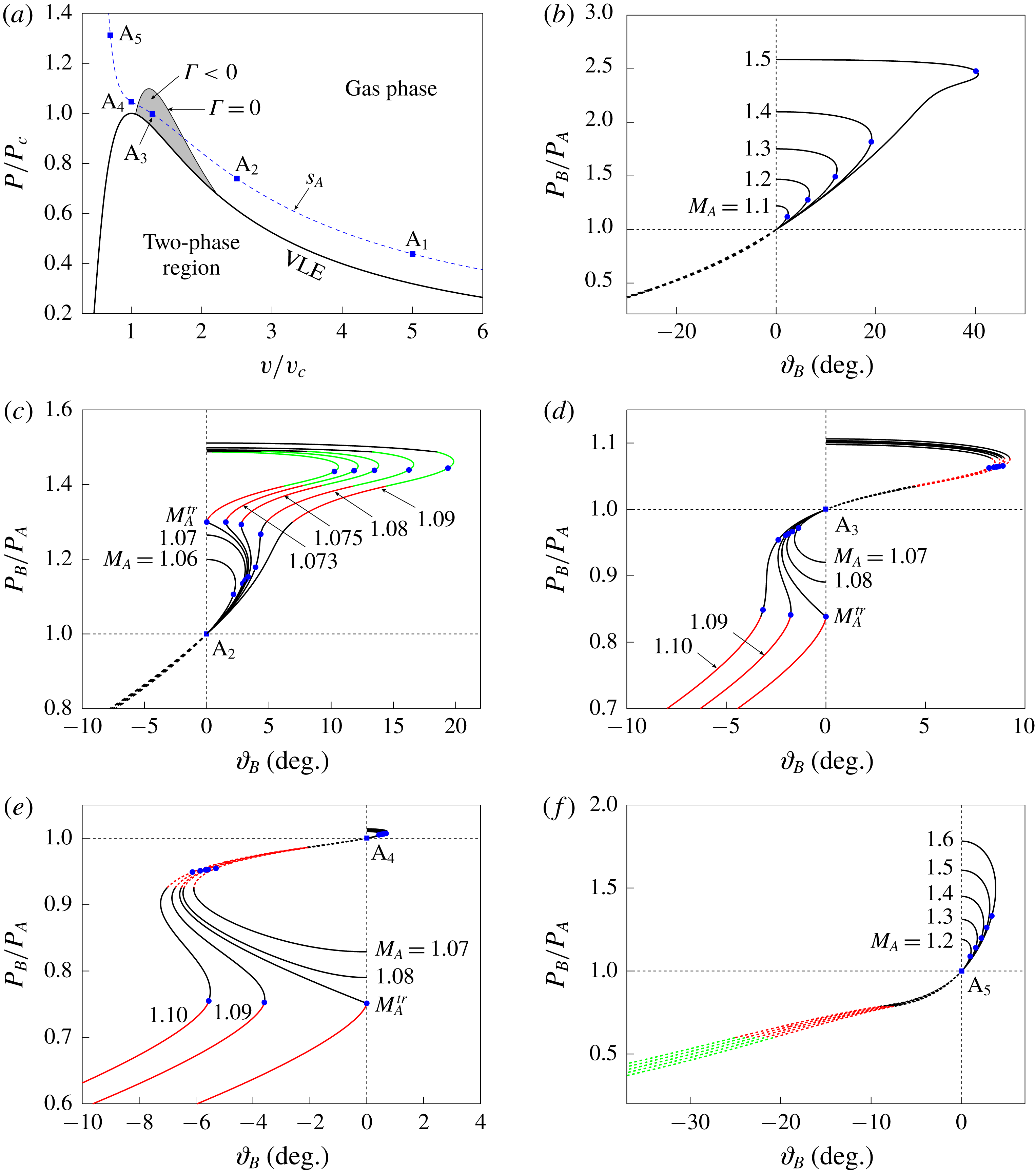In order to analyse the possible configurations of the wave curves along with the influence of $M_{A}$ , we select the same upstream thermodynamic states considered in the previous section and we draw the wave-curve projection in the $P_{B}$ – $\unicode[STIX]{x1D717}_{B}$ diagram for different values of $M_{A}$ , as shown in figure 2. Without loss of generality, only left-running wave curves are considered, as the right-running wave is just the reflection, through the $\unicode[STIX]{x1D717}_{B}=0$ axis, of the left-running counterpart.

Case 1 – figure 2(b). On a qualitative basis, this is the classical case. The rarefaction branch (Prandtl–Meyer waves) extends to vacuum conditions (eventually the saturated phase boundary is crossed), where the deflection angle attains a finite limit value. The pressure rise along the compression branch is limited by the normal shock wave ( $\unicode[STIX]{x1D6FD}_{s}=90^{\circ },\unicode[STIX]{x1D717}_{B}=0$ ) from the upstream state. By increasing the upstream Mach number, and therefore the total enthalpy of the stream, the maximum pressure jump increases. As is well known (Thompson Reference Thompson1988, see, e.g.), for a given $\unicode[STIX]{x1D717}_{B}>0$ two oblique shocks can possibly occur, which are named the weak and the strong (based on the pressure jump) solutions.

Figure 2.

Left-running wave curves in the pressure–deflection diagram computed from the polytropic van der Waals model of fluid MDM. (a) The selected thermodynamic upstream states, chosen along an isentrope crossing the negative- $\unicode[STIX]{x1D6E4}$ region (shaded area). (b–f) Wave curves for each upstream thermodynamic state and different upstream Mach numbers. For each case, the downstream pressure $P_{B}$ is scaled using the corresponding upstream pressure $P_{A}$ . Wave configurations: —— (black) shock, —— (red) shock/fan, —— (green) shock/fan/shock, – – – (black) fan, – – – (red) fan/shock, – – – (green) fan/shock/fan. Symbol ● denotes downstream sonic points ( $M_{B}=1$ ).

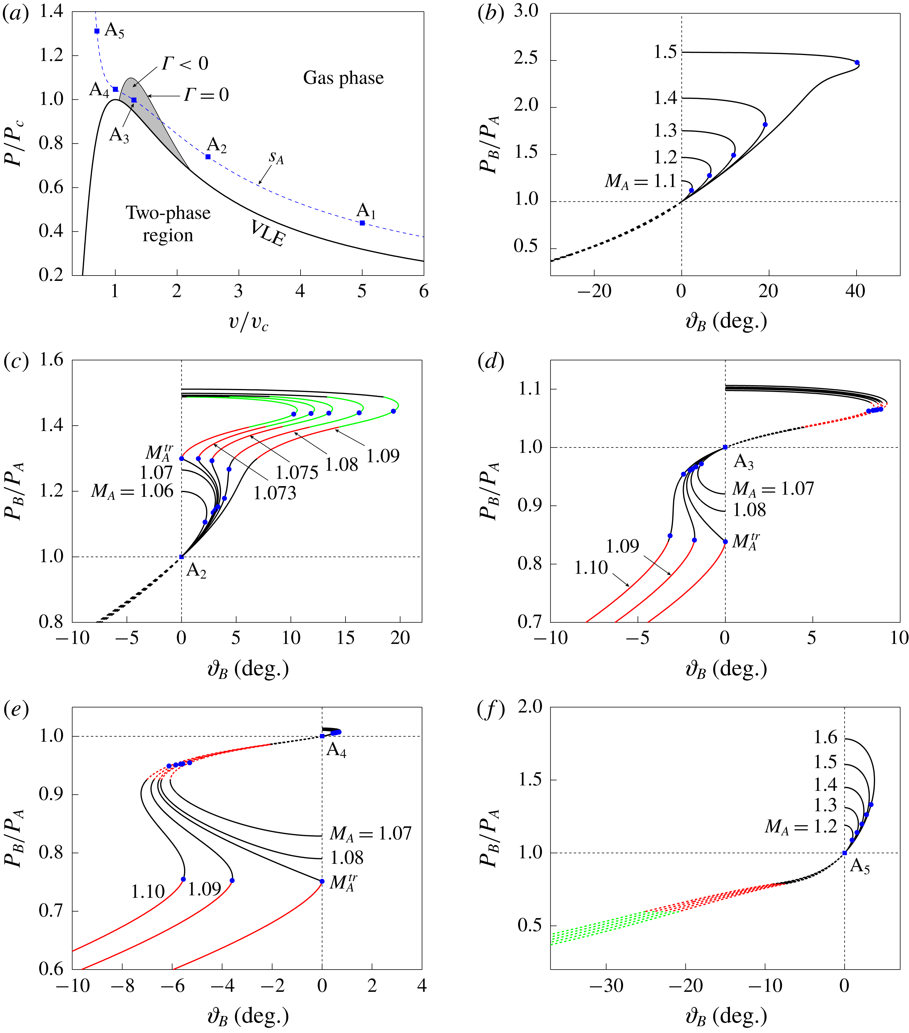
Case 2 – figure 2(c). While the rarefaction branch is qualitatively similar to case 1, there exists a limit value of the upstream Mach number, $M_{A}^{tr}$ , marking the transition between two qualitatively different compression-branch configurations. If $1<M_{A}<M_{A}^{tr}$ , the ordinary shock polar, similar to case 1, occurs. For $M_{A}>M_{A}^{tr}$ , along the compressive branch of the wave curve the following sequence is encountered, in the direction of increasing downstream pressure: oblique shock, oblique shock/Prandtl–Meyer fan, oblique shock/Prandtl–Meyer fan/oblique shock, oblique shock. The transitional wave curve is distinguished because the normal shock delimiting the first shock branch exhibits the sonic downstream state $M_{n\text{B}}=M_{B}=1$ , namely the post-shock thermodynamic state coincides with point $\text{S}^{+}$ in figure 1(c). By enforcing the Rankine–Hugoniot relations for a normal shock wave, the transitional Mach number is therefore computed as

(5.1) $$\begin{eqnarray}M_{A}^{tr}=\frac{1}{\unicode[STIX]{x1D70C}_{A}c_{A}}\sqrt{\frac{P_{S^{+}}-P_{A}}{v_{A}-v_{S^{+}}}},\end{eqnarray}$$

where $P_{S^{+}}$ and $v_{S^{+}}$ are the pressure and specific volume, respectively, at point $\text{S}^{+}$ . For upstream Mach numbers slightly larger than the transitional value, $\unicode[STIX]{x1D717}_{B}$ exhibits three stationary points along the wave curve (two local maxima with a minimum in between). Thus, up to four different wave configurations can provide the same flow deflection.

Case 3 – figure 2(d). A single qualitative configuration is observed for the compression side of the wave curve, which is composed by three branches: Prandtl–Meyer fan, Prandtl–Meyer fan/oblique shock, oblique shock (increasing downstream pressure). Two qualitatively different configurations are possible for the rarefaction branch, based on the value of the upstream Mach number. As in the previous case, a threshold Mach number $M_{A}^{tr}$ exists, such that the ordinary shock polar (although for rarefaction shocks) occurs if $M_{A}<M_{A}^{tr}$ . Note that, for $M_{A}<M_{A}^{tr}$ , the largest pressure drop is attained across the normal rarefaction shock from the upstream state, i.e. the rarefaction branch does not extend to vacuum. The transitional curve is again determined by the occurrence of a post-sonic normal shock wave (downstream thermodynamic state $S^{+}$ in figure 1 d). Therefore, formula (5.1) applies for the computation of $M_{A}^{tr}$ .

Case 4 – figure 2(e). The compression branch is the classical polar of oblique shocks. Two qualitatively different configurations of the rarefaction branch can possibly occur, again depending on $M_{A}$ . If $M_{A}<M_{A}^{tr}$ , the configurations are, in the direction of decreasing downstream pressure: Prandtl–Meyer fan, Prandtl–Meyer fan/oblique shock, oblique shock. If $M_{A}>M_{A}^{tr}$ , the wave curve extends to vacuum via an additional oblique shock/Prandtl–Meyer fan configuration. Similarly to cases 2 and 3, the transitional wave curve is distinguished by the occurrence of a post-sonic normal shock wave (downstream thermodynamic state $S^{+}$ in figure 1 e), so that $M_{A}^{tr}$ is again computed from relation (5.1).

Case 5 – figure 2(f). For case 5 a single wave-curve configuration is possible. The compression branch comprises the ordinary shock polar. For decreasing downstream pressures, the rarefaction branch consists of: Prandtl–Meyer fan, Prandtl–Meyer fan/oblique shock, Prandtl–Meyer fan/oblique shock/Prandtl–Meyer fan.

All the above shock solutions satisfy the stability conditions specified in § 2.2. However, it was shown by Kontorovich (Reference Kontorovich1958) that in the range

(5.2) $$\begin{eqnarray}{\displaystyle \frac{1-M_{n+}^{2}-(v_{-}/v_{+})M_{n+}^{2}}{1-([v]/v_{+})M_{n+}^{2}}}<-\frac{[P]}{[v]}\left(\left.\frac{\text{d}P}{\text{d}v}\right|_{+}\right)^{-1}\leqslant 1+2M_{n+}\end{eqnarray}$$

the shock front is only neutrally stable against transverse perturbations and can spontaneously emit acoustic waves (see also Fowles Reference Fowles1981). Acoustic emission is predicted to occur in molecularly complex fluids, for shock waves originating in the thermodynamic region close to the saturation curve and critical point (Alferez & Touber Reference Alferez and Touber2017). We note that inequalities (5.2) are satisfied if the sonic point in the pressure–deflection polar is at larger pressures than the maximum turning angle (Menikoff & Plohr Reference Menikoff and Plohr1989). One such case is the oblique shock polar marked by $M_{A}=1.5$ in figure 2(b).

6 Upstream-state map of the wave-curve types

Having described the different configurations of the compression and rarefaction branches of the waves curves for steady, two-dimensional and supersonic (possibly mixed supersonic/subsonic across strong oblique shocks) flows, we can now investigate the necessary conditions that the upstream state must satisfy in order to produce a specific wave-curve configuration. Ultimately, the purpose of this section is to determine a map of the upstream states leading to the different types of wave curves identified in the previous section.

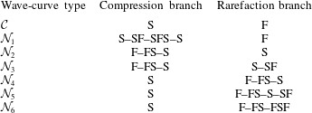
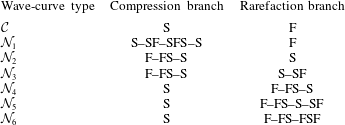
For future convenience, the wave-curve types are classified according to their qualitative structure, as shown in table 1. Seven different wave-curve configurations are singled out, which include the classical configuration ${\mathcal{C}}$ and six different non-classical configurations ${\mathcal{N}}_{i}$ , $i=1,\ldots ,6$ . The classical wave curve ${\mathcal{C}}$ is the one depicted in figure 2(b) and in figure 2(c) for $M_{A}<M_{A}^{tr}$ ; ${\mathcal{N}}_{1}$ is found in 2(c) if $M_{A}>M_{A}^{tr}$ ; ${\mathcal{N}}_{2}$ and ${\mathcal{N}}_{3}$ occur in figure 2(d) for $M_{A}<M_{A}^{tr}$ and $M_{A}>M_{A}^{tr}$ , respectively; ${\mathcal{N}}_{4}$ and ${\mathcal{N}}_{5}$ in figure 2(e) for $M_{A}<M_{A}^{tr}$ and $M_{A}>M_{A}^{tr}$ , respectively; finally ${\mathcal{N}}_{6}$ is the configuration shown in figure 2(f).

Figure 3.

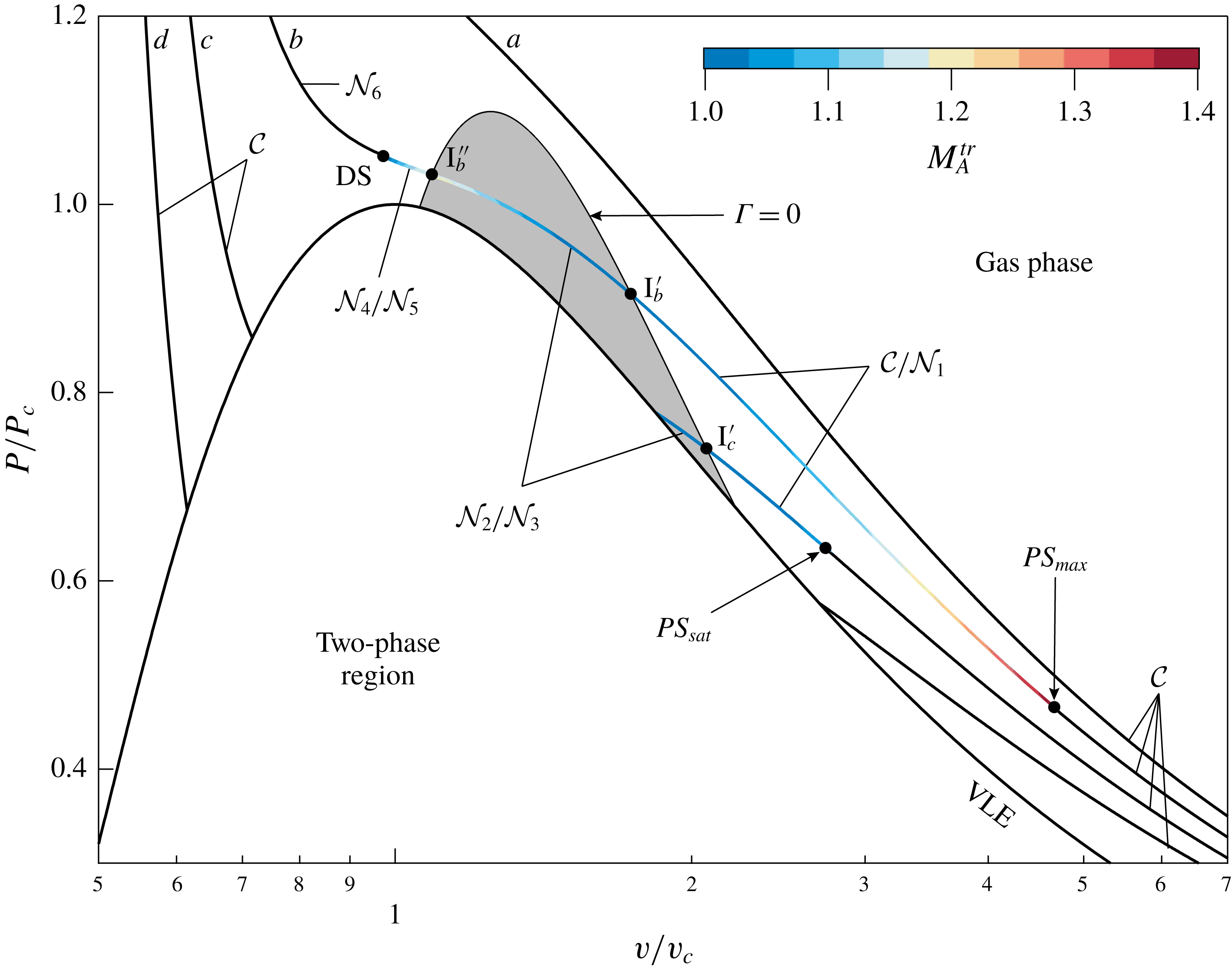
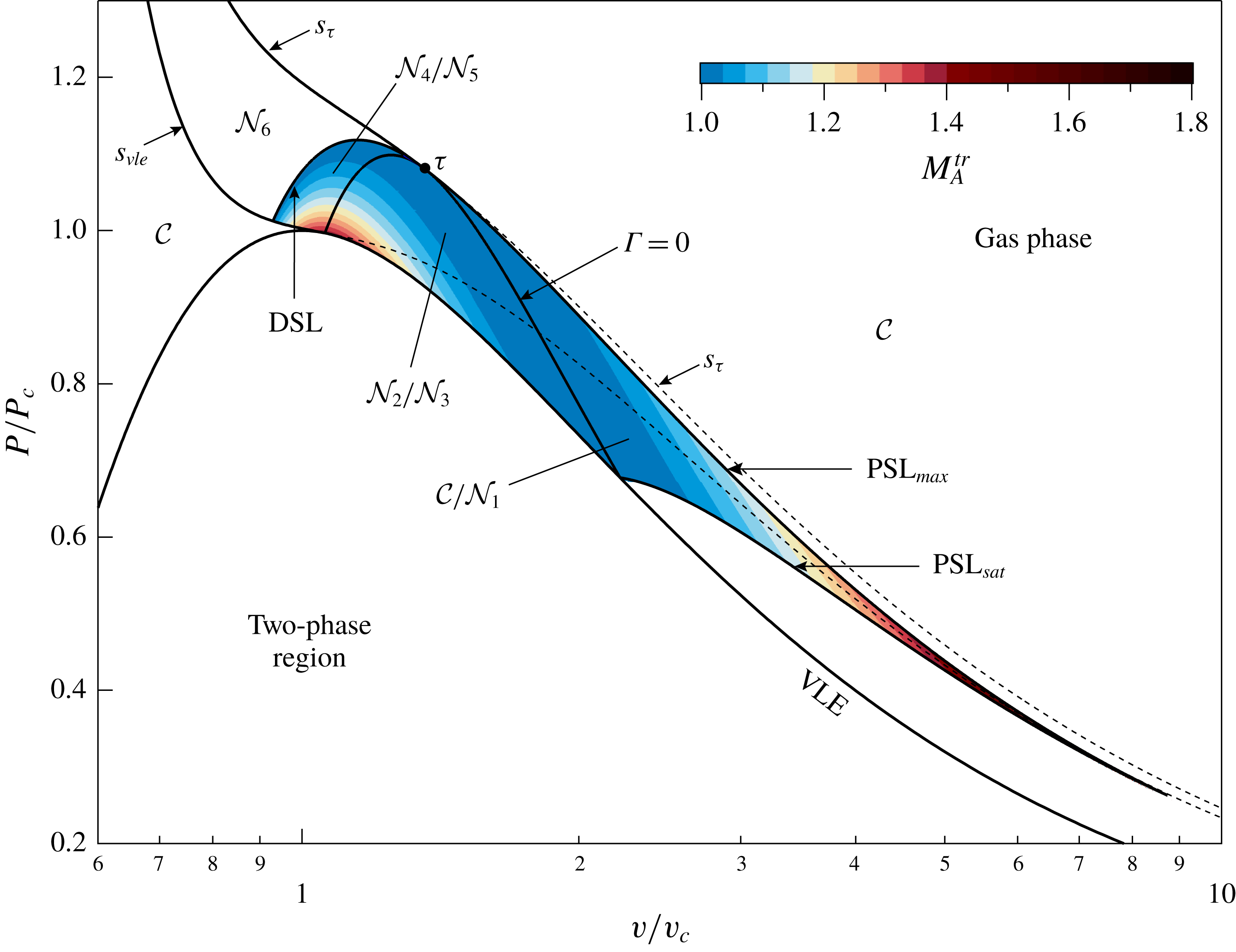
Wave-curve configurations for upstream thermodynamic states along selected isentropes, as computed from the polytropic van der Waals model of fluid MDM. The colour map indicates the transitional upstream Mach number (cf. relation (5.1)) for the branches where two different configurations are possible.

Table 1.

Classification of the wave curves. S: oblique shock; F: Prandtl–Meyer fan; SF: composite oblique shock/Prandtl–Meyer fan; SFS: composite oblique shock/Prandtl–Meyer fan/oblique shock; FS: composite Prandtl–Meyer fan/oblique shock; FSF: composite Prandtl–Meyer fan/oblique shock/Prandtl–Meyer fan. In the compression branch, the configurations encountered are listed in the order of increasing downstream pressure, while in the rarefaction branch they are in the order of decreasing downstream pressure.

In order to reduce the complexity associated with the dependence of the wave curves on three upstream quantities (two thermodynamic quantities, e.g. $P_{A}$ , $v_{A}$ and a kinematic or mixed one, e.g. $M_{A}$ ), we first consider upstream thermodynamic states along exemplary isentropes, as shown in figure 3, and we analyse the conditions that determine the transition between different wave-curve configurations.

Isentrope $a$ in figure 3 is representative of the scenario observed for convex isentropes. As such, only classical wave curves can originate from upstream thermodynamic states along these curves and any given upstream Mach number $M_{A}>1$ .

Isentrope $b$ is the same used for the parametric studies of the previous sections. It is representative of the scenario arising from isentropes that cross the negative- $\unicode[STIX]{x1D6E4}$ region while remaining in the single phase. At sufficiently low upstream pressures, only the classical configuration shown in figures 1(b) and 2(b) can occur. By increasing the pressure along the selected isentrope, point $\text{PS}_{max}$ is encountered at which the wave curve first includes a post-sonic compression shock. It can be shown (Menikoff & Plohr Reference Menikoff and Plohr1989) that the post-sonic compression shock arising from $\text{PS}_{max}$ exhibits $\unicode[STIX]{x1D6E4}_{B}=0$ . Also, it is the post-sonic compression shock of largest intensity (e.g. pressure or entropy jump) among those originating from the selected isentrope. For pressures included between $\text{PS}_{max}$ and $\text{I}_{b}^{\prime }$ (low-density intersection with the $\unicode[STIX]{x1D6E4}=0$ locus), the extended wave curve in the thermodynamic plane is qualitatively similar to that of figure 1(c). As shown in § 5, two different types of wave curve ( ${\mathcal{C}}$ and ${\mathcal{N}}_{1}$ ) can occur based on the value of the upstream Mach number. The threshold Mach number between these two configurations, as computed from relation (5.1), is graphically highlighted in figure 3 using the colour map. For upstream states exhibiting $\unicode[STIX]{x1D6E4}_{A}<0$ , wave curves of type ${\mathcal{N}}_{2}$ or ${\mathcal{N}}_{3}$ can be observed. The same transitional criterion based on $M_{A}$ applies and is again represented on the selected isentrope in figure 3. The branch of isentrope $b$ on the left-hand side of point $\text{I}_{b}^{\prime \prime }$ (high-density intersection with the $\unicode[STIX]{x1D6E4}=0$ locus), is divided in two sections by point DS, which denotes the occurrence of a double-sonic shock (Zamfirescu et al. Reference Zamfirescu, Guardone and Colonna2008). Between $\text{I}_{b}^{\prime \prime }$ and DS, double-sonic shocks from upstream states along the chosen isentrope are not possible. Therefore, configurations ${\mathcal{N}}_{4}$ or ${\mathcal{N}}_{5}$ can occur based on $M_{A}$ . Beyond point DS, the wave curve is of type ${\mathcal{N}}_{6}$ only.

In the present discussion, we also consider the single-phase portions of isentropes crossing the saturation curve. The case of isentropes crossing both the negative- $\unicode[STIX]{x1D6E4}$ region and the saturation curve is the one labelled $c$ in figure 3. Non-classical configurations can possibly exist only in the neighbourhood of point $\text{I}_{c}^{\prime }$ . The branch ${\mathcal{C}}/{\mathcal{N}}_{1}$ , in this case, is bounded below by point $\text{PS}_{sat}$ , where the post-sonic shock required for the existence of ${\mathcal{N}}_{1}$ configurations features post-shock saturated conditions (namely, the post-shock thermodynamic state lies on the vapour–liquid equilibrium curve). Finally, for isentropes such as case $d$ in figure 3, which cross the phase boundary but do not cross the negative- $\unicode[STIX]{x1D6E4}$ region, only the classical wave-curve configuration is predicted to occur.

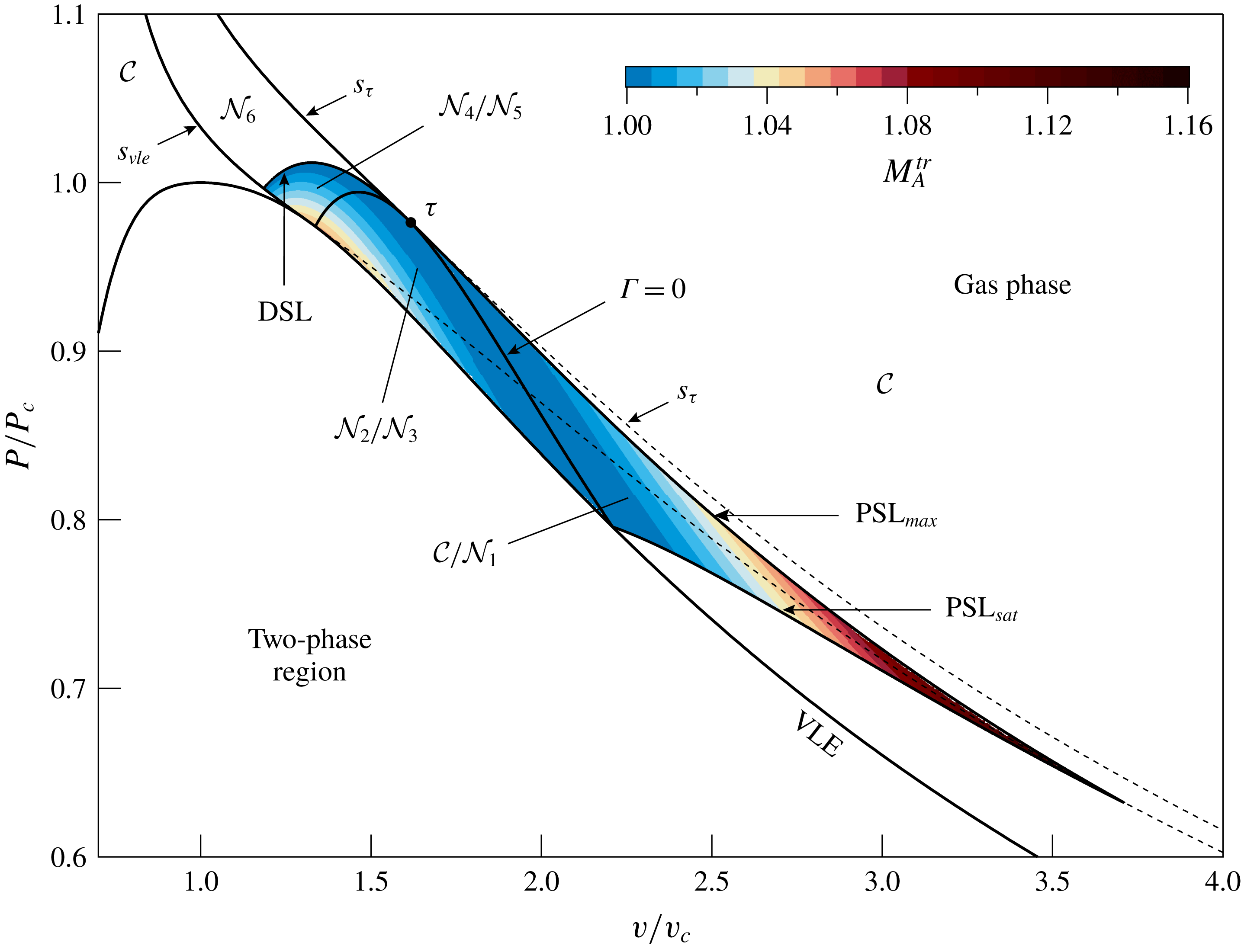
By applying the above procedure to each possible isentrope, a map of the upstream states leading to each wave-curve configuration is obtained in terms of thermodynamic quantities and Mach number, see figure 4. In the $P$ – $v$ plane, the thermodynamic region associated with non-classical wave curves is bounded above by the isentrope $s_{\unicode[STIX]{x1D70F}}$ tangent to the $\unicode[STIX]{x1D6E4}=0$ locus and by the curve $\text{PSL}_{max}$ . The latter is obtained by collecting all the upstream states $\text{PS}_{max}$ leading to post-sonic shocks of maximal intensity along a given pre-shock isentrope (as defined above). In a similar fashion, the curve $\text{PSL}_{sat}$ is computed as the locus of thermodynamic states $\text{PS}_{sat}$ , for each isentrope crossing both the negative- $\unicode[STIX]{x1D6E4}$ region and the saturation curve. The $\text{PSL}_{sat}$ bounds from below the region for non-classical wave curves, along with the saturation curve itself and the isentrope $s_{vle}$ tangent to the latter. The locus $\unicode[STIX]{x1D6E4}=0$ marks the transition between the regions ${\mathcal{C}}/{\mathcal{N}}_{1}$ and ${\mathcal{N}}_{2}/{\mathcal{N}}_{3}$ and between the regions ${\mathcal{N}}_{2}/{\mathcal{N}}_{3}$ and ${\mathcal{N}}_{4}/{\mathcal{N}}_{5}$ . The DSL curve, which separates the regions ${\mathcal{N}}_{4}/{\mathcal{N}}_{5}$ and ${\mathcal{N}}_{6}$ , is obtained by collecting the pre-shock states of double-sonic shocks (DS). The DSL shown in figure 4 is indeed a portion of the double-sonic locus defined by Zamfirescu et al. (Reference Zamfirescu, Guardone and Colonna2008). Outside the above-described region, only classical wave curves can take place.

Figure 4.

Upstream-state map of the wave curves in the $P$ – $v$ plane, as computed from the polytropic van der Waals model of fluid MDM. Superposed is the value of transitional upstream Mach number (cf. relation (5.1)) for the regions where two different configurations are possible.

We assert that the present findings do not depend on the specific choice of the thermodynamic model, insofar as they result from the existence of a finite negative- $\unicode[STIX]{x1D6E4}$ region in the vapour phase. To support this claim, the upstream-state map of the wave curves for fluid $\text{MD}_{4}\text{M}$ (tetradecamethylhexasiloxane, $\text{C}_{14}\text{H}_{42}\text{O}_{5}\text{Si}_{6}$ ), as computed from the state-of-the-art multi-parameter equation of state of Thol et al. (Reference Thol, Javed, Baumhoegger, Span and Vrabec2018) available via the REFPROP library (Lemmon, Huber & McLinden Reference Lemmon, Huber and McLinden2013), is reported in figure 5 and shows excellent qualitative agreement with the picture given by the simple van der Waals model.

Figure 5.

Upstream-state map of the wave curves in the $P$ – $v$ plane, as computed from the reference thermodynamic model of fluid $\text{MD}_{4}\text{M}$ (Thol et al. Reference Thol, Javed, Baumhoegger, Span and Vrabec2018), available via the REFPROP library (Lemmon et al. Reference Lemmon, Huber and McLinden2013). Superposed is the value of transitional upstream Mach number (cf. relation (5.1)) for the regions where two different configurations are possible.

7 Concluding remarks

The general properties of self-similar oblique waves (left running or right running with respect to the fluid particle velocity) in steady, inviscid, single-phase Bethe–Zel’dovich–Thompson vapours were studied. The developed theoretical framework concentrates on compressive and rarefactive ramps/wedges in both the classical and non-classical gas dynamic context, which are the building blocks of steady planar supersonic flows. Due to the possibly non-convex character of isentropes and shock adiabats in the pressure–specific volume diagram, several oblique-wave patterns arise which are not admissible in the classical theory of gas dynamics. These are composite shock/fan, fan/shock, shock/fan/shock and fan/shock/fan combinations. Moreover, the elementary oblique waves originating from thermodynamic states in the negative- $\unicode[STIX]{x1D6E4}$ region exhibit inverse gas dynamic behaviour, namely oblique shocks carry an expansion while Prandtl–Meyer fans are compressive.

The two-dimensional ramp problem was described moving from the one-dimensional Riemann problem, thus allowing us to exploit most of the techniques developed for self-similar flow in one dimension. Accordingly, the concept of wave curve for steady two-dimensional flow, which is the counterpart the wave curve in the one-dimensional Riemann problem, was introduced. Within the present context, the wave curve consists of all the states (in terms of thermodynamic and kinematic quantities) that can possibly be connected to a given supersonic state by means of a steady, two-dimensional and self-similar wave. A two-step procedure was adopted to compute the wave curve: the projection onto the thermodynamic variables was first considered, since it represents a subset of the unsteady one-dimensional counterpart, and afterwards all the kinematic quantities were retrieved.

The different types of wave curves were illustrated my means of a parametric study in the space of the upstream thermodynamic quantities (e.g. pressure and specific volume) and Mach number, using the van der Waals gas model (with constant isochoric specific heat) of a molecularly complex fluid. Seven different wave-curve configurations were singled out, which include the classical case ( ${\mathcal{C}}$ ) and six non-classical cases ( ${\mathcal{N}}_{1}$ , ${\mathcal{N}}_{2}$ , ${\mathcal{N}}_{3}$ , ${\mathcal{N}}_{4}$ , ${\mathcal{N}}_{5}$ , ${\mathcal{N}}_{6}$ ). The conditions leading to the transition between the different types of wave curve were analysed. This led to the definition of a map, in the parameter space of the thermodynamic quantities and Mach number, of the upstream states leading to each type of wave curve. Most important, it was shown that the domain of the thermodynamic states leading to wave curves of non-classical type is significantly larger than the negative- $\unicode[STIX]{x1D6E4}$ region in which inverse gas dynamic behaviour is expected to occur. As the peculiar oblique-wave properties stem from the occurrence of a negative- $\unicode[STIX]{x1D6E4}$ region in the vapour phase, we expect that the results obtained from the simple van der Waals model apply to diverse thermodynamic models of BZT fluids. The computation of the upstream-state map of the wave curves using the state-of-the-art thermodynamic model of fluid $\text{MD}_{4}\text{M}$ corroborates this statement.

In contrast with the classical case, if the non-classical configuration ${\mathcal{N}}_{1}$ is generated, up to four different wave patterns corresponding to the same ramp angle can possibly occur. Moreover, for the non-classical configurations ${\mathcal{N}}_{2}$ , ${\mathcal{N}}_{3}$ , ${\mathcal{N}}_{4}$ and ${\mathcal{N}}_{5}$ , the deviation angle does not vary monotonically with the downstream pressure along the expansion branch, where up to three different wave patterns can possibly occur which correspond to the same ramp angle.

Among others, an important problem for further study is the stability of oblique waves in the ramp configuration, which is required for the experimental observation of these non-classical phenomena, see Kluwick & Cox (Reference Kluwick and Cox2018). In closing, we note that the current theoretical framework can be conveniently applied to the study of shock reflections and shock interactions, which will be the topic of future studies.