The word dyad is widespread in the international relations (IR) literature. Its first use in the political science literature appears to be from Rudolph J. Rummel's work in the 1960s.Footnote 1 Statisticians had been analyzing dyadic data at least since Fisher (Reference Fisher1925), and sociologists had used the term by the late 19th century (Tönnies Reference Tönnies1887); it even appears in sociological textbooks throughout the 19th century (Simmel Reference Simmel1908).Footnote 2
Since the introduction of dyads into the political science literature, they have been extensively used as a framework for analyzing pairs of countries, taking each pair seriatim. Scholars sought to determine which dyads were dangerous (Bremer Reference Bremer1992), which sets of dyads were politically relevant (Gasiorowski and Polachek Reference Gasiorowski and Polachek1982; Maoz and Russett Reference Maoz and Russett1993), which were relevant (Lemke and Reed Reference Lemke and Reed2001) and even which dyads were jointly democratic (Reuveny and Li Reference Reuveny and Li2003).
The dyad has become ubiquitous. Early work in IR focused on the behavior and policies of individual states (for example, Morgenthau Reference Morgenthau1948). Subsequent work focused on the relationship of those individual states to a system (for example, Kaplan Reference Kaplan1957), and some work focused entirely on the system (for example, McClelland Reference McClelland1967). Most contemporary empirical work has focused on analyzing data on dyads. This includes work on the democratic peace that invented dyadic covariates such as the level of democracy in the dyad (vide Maoz and Russett Reference Maoz and Russett1993; Rousseau et al. Reference Rousseau, Gelpi, Reiter and Huth1996), as well as work on the dynamics of conflict more generally (Russett, Oneal and Davis Reference Russett, Oneal and Davis1998; King Reference King2001; Gartzke and Gleditsch Reference Gartzke and Gleditsch2004). Much of this analysis of the so-called democratic peace has adopted a dyadic design that is by now not only catholic, but that has not changed since it was first introduced. Indeed, the March 2013 issue of the International Studies Quarterly contains three articles that use a dyadic design (Gartzke and Weisiger Reference Gartzke and Weisiger2013; Mousseau Reference Mousseau2013; Dafoe, Oneal and Russett Reference Dafoe, Oneal and Russett2013). Dyads have also been used to analyze a wide variety of variables, beyond conflicts and militarized disputes, including investment (Elkins, Guzman and Simmons Reference Elkins, Guzman and Simmons2006). Recent work on trade mostly uses a dyadic perspective (Tomz, Goldstein and Rivers Reference Tomz, Goldstein and Rivers2007; Rose Reference Rose2007), and the dyadic perspective is growing in the area of civil war studies as well (Salehyan and Gleditsch Reference Salehyan and Gleditsch2006; Cunningham, Gleditsch and Salehyan Reference Cunningham, Gleditsch and Salehyan2009).Footnote 3
For the most part, however, dyadic research in IR ignores the essential features of dyads in that they fail to satisfy the assumption of independence or, by construction, have missing data but ignore its effects—both of which fundamentally bias the results. Most contemporary political science research on dyadic data use one of these two approaches, resulting in a data analysis file in which the rows of the data are either individual dyad-pairs or dyads themselves, with data on both the actor and the partner inside each row. Analysis typically proceeds under the assumption that the rows thus constructed are independent of one another, or that any biases that are introduced can be corrected via post-estimation adjustments to the variance estimates. This is the standard approach, in which an ordinary least squares analysis is run and the standard errors are clustered.Footnote 4 In this approach, the standard errors might apply to coefficients for dyads or countries, depending on the time domain of the analysis.Footnote 5
We demonstrate that the Social Relations Model (SRM) provides a straightforward and systematic approach that focuses on, rather than avoids, the interdependencies that exist in the relationships among different actors within organizations and groups. Most notably, the SRM allows for an easy interpretation of variance in the network. By decomposing the variance, we can better understand which effects (that is, actor or partner effects) capture the greatest proportion of total variance in the network. Next, we present the SRM as a direct approach for addressing these effects and incorporating their analysis into the future IR literature.
The Social Relations Model
The SRM was established as a way to focus on, rather than avoid, the interdependencies that exist in the relationships among individuals in a family or social group. If individuals i and j interact, it is plausible that j's characteristics will influence i's actions, and vice versa. Their joint, or dyadic, characteristics will also influence what happens between them. This is the basis of Kenny's SRM, which is a simple approach with widespread currency in social psychology (Kenny, Kashy and Cook Reference Kenny, Kashy and Cook2006; Kenny Reference Kenny1994).
The SRM method decomposes the variance of such data into sender and receiver effects, and permits within-dyad correlations via the analysis of variance (ANOVA) protocol (Warner, Kenny and Stoto Reference Warner, Kenny and Stoto1979; Gill and Swartz Reference Gill and Swartz2001). The development of the SRM is presented first by Kenny (Reference Kenny1981), but the canonical citation is from the mid-1980s (Malloy and Kenny Reference Malloy and Kenny1986). A widely cited volume was penned on this topic in the mid-1990s (Kenny Reference Kenny1994), and a book devoted to data analytic approaches to the SRM was published in the last decade (Kenny, Kashy and Cook Reference Kenny, Kashy and Cook2006). It grew out of psychologists’ interest in separating the independent and interactive effects of groups versus individuals. The basic insight provides a way of conceptualizing and acquiring unbiased estimates of actor, partner and relationship effects and their interrelationships. The idea of further decomposing the variance in the context of dyadic data was developed (Gill and Swartz Reference Gill and Swartz2001; Li and Loken Reference Li and Loken2002) to permit the statistical analysis of normally distributed dyadic data using additive effects. These ideas have been extended to a generalized linear model that incorporates third-order dependence via a bilinear effect (Hoff Reference Hoff2005) similar to that introduced by Gabriel (Reference Gabriel1998).Footnote 6
We begin first, however, with an illustration of the SRM decomposition in which we have six actors in a round robin (dyadic) format. These data are represented by the matrix Xij, which has the measured value of each of the 30 interactions, with the diagonal remaining empty:
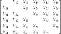 $$\left[ \matrix{ {} & {{{X}_{{\rm{12}}}}} & {{{X}_{{\rm{13}}}}} & {{{X}_{{\rm{14}}}}} & {{{X}_{{\rm{15}}}}} & {{{X}_{{\rm{16}}}}} \cr {{{X}_{{\rm{21}}}}} & {} & {{{X}_{{\rm{23}}}}} & {{{X}_{{\rm{24}}}}} & {{{X}_{{\rm{25}}}}} & {{{X}_{{\rm{26}}}}} \cr {{{X}_{{\rm{31}}}}} & {{{X}_{{\rm{32}}}}} & {} & {{{X}_{{\rm{34}}}}} & {{{X}_{{\rm{35}}}}} & {{{X}_{{\rm{36}}}}} \cr {{{X}_{{\rm{41}}}}} & {{{X}_{{\rm{42}}}}} & {{{X}_{{\rm{43}}}}} & {} & {{{X}_{{\rm{45}}}}} & {{{X}_{{\rm{46}}}}} \cr {{{X}_{{\rm{51}}}}} & {{{X}_{{\rm{52}}}}} & {{{X}_{{\rm{53}}}}} & {{{X}_{{\rm{54}}}}} & {} & {{{X}_{{\rm{56}}}}} \cr {{{X}_{{\rm{61}}}}} & {{{X}_{{\rm{62}}}}} & {{{X}_{{\rm{63}}}}} & {{{X}_{{\rm{64}}}}} & {{{X}_{{\rm{65}}}}} &} \right]$$
To get at the actor and dyadic effects, we must first calculate various means. These begin with calculating the row column and total sums. The totals for each row are denoted Xi. where i is the row number:
 $${{X}_{i \cdot }}\, = \,\mathop{\sum}\limits_{j\, = \,{\rm{1}}}^J {{X}_{ij}}.$$
For each column, the totals are denoted X.i where i is the column number, and the total over all rows and columns is:
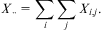 $${{X}_{ \cdot \cdot }}\, = \,\mathop{\sum}\limits_i \mathop{\sum}\limits_j {{X}_{i,j}}.$$
Using this method, one can calculate individual effects for a variety of interesting concepts, such as the actor, partner and unique dyadic effects (as well as the variances attributed to each of these effects). Such concepts are missing from a standard regression approach to analyzing dyadic data.
The actor effect for observation i is the total of i's row mean and column mean, minus the overall mean. The means are just the sums, corrected for degrees of freedom, yielding an average row effect:
 $${{\hat{a}}_i}\, = \,\frac{{{{{(n\,{\rm{ - }}\,{\rm{1}})}}^{\rm{2}}} }}{{n(n\,{\rm{ - }}\,{\rm{2}})}}{{X}_{i \cdot }}\, + \,\frac{{(n\,{\rm{ - }}\,{\rm{1}})}}{{n(n\,{\rm{ - }}\,{\rm{2}})}}{{X}_{ \cdot i}}\,{\rm{ - }}\,\frac{{n\,{\rm{ - }}\,{\rm{1}}}}{{n\,{\rm{ - }}\,2}}{{X}_{ \cdot \cdot }}.$$
Similarly the column mean for actor i is:
 $${{\hat{b}}_i}\, = \,\frac{{{{{(n\,{\rm{ - }}\,{\rm{1}})}}^{\rm{2}}} }}{{n(n\,{\rm{ - }}\,{\rm{2}})}}{{X}_{ \cdot i}}\, + \,\frac{{(n\,{\rm{ - }}\,{\rm{1}})}}{{n(n\,{\rm{ - }}\,{\rm{2}})}}{{X}_{i \cdot }}\,{\rm{ - }}\,\frac{{n\,{\rm{ - }}\,{\rm{1}}}}{{n\,{\rm{ - }}\,2}}{{X}_{ \cdot \cdot }}.$$
For a symmetric matrix, the row and column effects will be identical, by construction. Finally, the unique dyadic effect for each specific dyad ij simply subtracts the row and column effects along with the overall mean out of the value for dyad ij:
 $${{\hat{g}}_{ij}}\, = \,{{X}_{ij}}\,{\rm{ - }}\,{{\hat{a}}_i}\,{\rm{ - }}\,{{\hat{b}}_j}\,{\rm{ - }}\,{{X}_{ \cdot \cdot }}$$
These formulae are simple, but need some explication. Imagine that the data are the perceived hostility among six groups of anti-government actors. Suppose we want to assess how actor i perceives the others. We can do this by averaging the scores for other group members, but we must correct for the possibility that although actor i may not perceive himself/herself as hostile, others might. This is corrected by including a measure of the average hostility of i as perceived by other members in the set. Thus the actor effect ( $$${{\hat{a}}_i}$$$
) is equal to the row mean of individual i, plus the column mean of individual i, minus the grand mean across all individuals, each of these three quantities controlled for the correct number of cases.
Similarly, one can calculate the partner and dyadic effects. The latter consists of the dyadic effect of i toward j, removing the tendency of i to view others as hostile and removing the average tendency for j to be viewed as hostile. The overall group mean is also subtracted from this individual effect. The result consists of effects that are unique to the dyad, and not accounted for in actor or partner effects.
These quantities are descriptive and helpful in understanding how the dependencies among actors may be understood from the available network data. And, subsequently, we can model the means. But first, we need to also examine the formulae for the variances. Following the logic of calculating the means for actors, targets and dyads, we can derive simple formulae for the variances and covariances, which follow directly from these quantities. Such quantities of interest are easy to derive as well, as shown herewith:
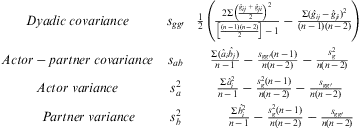 $$\matrix{ {Dyadic\;covariance} & {{{s}_{gg{\prime}}}} & {\frac{{\rm{1}}}{{\rm{2}}}\left( {\frac{{{\rm{2}}\rSigma {{{\big(\frac{{{{{\hat{g}}}_{ij}}\, + \,{{{\hat{g}}}_{ji}}}}{{\rm{2}}}\big)}}^{\rm{2}}} }}{{\big[\frac{{(n\,{\rm{ - }}\,{\rm{1}})(n\,{\rm{ - }}\,{\rm{2}})}}{{\rm{2}}}\big]\,{\rm{ - }}\,{\rm{1}}}}\,{\rm{ - }}\,\frac{{\rSigma {{{({{{\hat{g}}}_{ij}}\,{\rm{ - }}\,{{{\hat{g}}}_{ji}})}}^{\rm{2}}} }}{{(n\,{\rm{ - }}\,{\rm{1}})(n\,{\rm{ - }}\,{\rm{2}})}}} \right)} \cr {Actor - partner\;covariance} & {{{s}_{ab}}} & {\frac{{\rSigma ({{{\hat{a}}}_i}{{{\hat{b}}}_j})}}{{n\,{\rm{ - }}\,{\rm{1}}}}\,{\rm{ - }}\,\frac{{{{s}_{gg{\prime}}}(n\,{\rm{ - }}\,{\rm{1}})}}{{n(n\,{\rm{ - }}\,{\rm{2}})}}\,{\rm{ - }}\,\frac{{s_{g}^{{\rm{2}}} }}{{n(n\,{\rm{ - }}\,{\rm{2}})}}} \cr {Actor\;variance} & {s_{a}^{{\rm{2}}} } & {\frac{{\rSigma \hat{a}_{i}^{{\rm{2}}} }}{{n\,{\rm{ - }}\,{\rm{1}}}}\,{\rm{ - }}\,\frac{{s_{g}^{{\rm{2}}} (n\,{\rm{ - }}\,{\rm{1}})}}{{n(n\,{\rm{ - }}\,{\rm{2}})}}\,{\rm{ - }}\,\frac{{{{s}_{gg{\prime}}}}}{{n(n\,{\rm{ - }}\,{\rm{2}})}}} \cr {\; \; \; \; \; \; Partner\;variance} & {s_{b}^{{\rm{2}}} } & {\; \; \; \; \; \; \frac{{\rSigma \hat{b}_{i}^{{\rm{2}}} }}{{n\,{\rm{ - }}\,{\rm{1}}}}\,{\rm{ - }}\,\frac{{s_{g}^{{\rm{2}}} (n\,{\rm{ - }}\,{\rm{1}})}}{{n(n\,{\rm{ - }}\,{\rm{2}})}}\,{\rm{ - }}\,\frac{{{{s}_{gg{\prime}}}}}{{n(n\,{\rm{ - }}\,{\rm{2}})}}} $$
By decomposing the variance we can assess which effects (the actor, partner or dyadic effects) account for most of the variance overall. A demonstration of the insights that such a breakdown of variance can provide is given in subsequent sections. The dyadic covariance is the amount of variability in the unique (dyadic) effects across all possible dyads ( $$$s_{g}^{2} $$$
). The actor-partner covariance, which has a similar formula, is the extent to which i's perception of j is correlated with j's perception of i. In the political science literature, this concept is frequently called reciprocity. In addition, we compute the actor and partner variances.
The point of this delineation—which draws especially on Card, Selig and Little (Reference Card, Selig and Little2008, chapter 11)—is to suggest that analyzing dyadic data can benefit from a more complete consideration of the interdependencies than is normally undertaken. But the simple univariate approach outlined above captures only part of the picture. It is mainly oriented toward what can be termed first- and second-order dependence. First-order dependence is easy to grasp, as it is the dependence of one observation directly on an adjacent one, and is often seen in a time series or spatial context. Second-order dependence refers to the reciprocity that may characterize the relationships among dyadic pairs: will aggressive behavior by India toward Pakistan engender a Pakistani response toward India? Similar to second-order dependence, third-order dependence is commonly addressed in the literature of social network analysis. Important components of this higher-order dependence include transitivity, balance and clusterability. We further address these types of higher-order dependencies in the latter half of this article.
The Srm Put Into Practice
The SRM differs from other contributions to the IR literature on interdependence. The Exponential Random Graph Model (ERGM) is one approach to handling some of issues relevant to interdependence in IR. The ERGM is a statistical model that can estimate the effects of covariates on the ties in a network and, at the same time, estimate the dependencies in the network. Unlike the SRM, ERGM models are generally limited to analysis of binary data.Footnote 7
In the context of geographical models, Neumayer and Plümper (Reference Neumayer and Plümper2010) elaborate some of the issues related to the interdependence of observations across space. Hays, Kachi and Franzese (Reference Hays, Kachi and Franzese2010) produce spatial weights that capture the degree of connection between country i and country j. After constructing spatial weights, they normalize them to provide a non-uniform weight matrix that can be used in regression analysis. The SRM can be applied to many types of theoretical and empirical problems, including questions of spatial dependence.
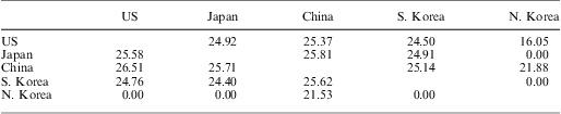
Consider the manufacturing exports among five countries in 2011. These are presented (in logs) in Table 1. The actor means are 22.71 (United States), 19.07 (Japan), 24.81 (China), 18.70 (South Korea) and 5.38 (North Korea). Applying the formulae for actor effects shows, for example, that China and the United States (8.8 and 5.2, respectively) have the largest impact on this tiny trade network, and that they also have the greatest effect as trading partners (8.7 for China and 2.4 for the United States). However, the North Korean dyad with China has a unique effect (10.6) that is almost an order of magnitude larger than other dyadic effects.
Manufacturing Exports, 2011
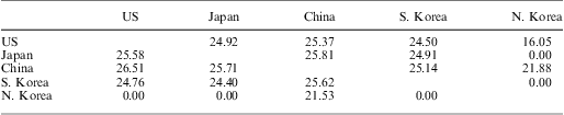
Note: data from the International Monetary Fund; in logs of millions of US dollars.
As Card, Selig and Little (Reference Card, Selig and Little2008) point out, the dyadic variance is difficult to interpret on its own, but it is most revealing when compared to the actor and partner variance, which enables us to more intuitively interpret the overall effect of the unique relationship variance. In our group of actors, we would find that the unique dyadic variance for the network of individuals is approximately 45 and the relationship covariance is about one-third less, 31. The relationship covariance can be thought of as the association between how country i perceives individual j as an active trader and how partner j perceives country i as active in trading. Dividing the relationship covariance by the relationship variance we find the correlations between the two, which in this case is roughly 0.7. None of these effects is captured in the standard dyadic research design found in the IR literature.Footnote 8
Snijders and Kenny (Reference Snijders and Kenny1999) showed how multilevel models can be used to study dyadic variables using an SRM approach with covariates by using a type of hierarchical linear model. In the next section, we also use a type of mixed-effect modeling to implement the SRM in the context of dyadic network data to explain theoretically important phenomenon in IR.Footnote 9
International Relations
We use three examples to illustrate how our version of dyadic analysis adds additional insight beyond the dyadic analysis that is typically employed in IR: analysis of Militarized Interstate Disputes (MIDs), international trade and the reciprocity inherent in the treatment of prisoners of war (POWs).
Militarized Interstate Disputes
We turn now to an analysis of one of the canonical datasets for IR, the MID data, which was collected by the Correlates of War project and widely employed in empirical studies of IR. We use the SRM to analyze the dependencies in dyadic data for international conflict annually from 1816–2001. We break down this data in three different ways. First, we create an aggregated matrix representing the years 1952–2001. This matrix mirrors much of the work done in IR, where data on conflictual interactions is treated as binary. Secondly, because the SRM can support a variety of data types, we create another version of the aggregated matrix that contains counts of the number of dispute onsets over the 50-year period (that is, a running count of whether there was an MID in a given year). Thus if country i initiates three different disputes during the 50-year period against country j (or is on the side of an initiator), then a count of 3 is shown in the aggregated matrix for Xij. We run the SRM on each of these aggregated matrices and report the results. Thirdly, we create an individual sociomatrix for each year of the MID data from 1816–2001. The rows and columns of each matrix represent the countries that existed in the international system for that year. The matrices then contain counts for each MID that occurred between any given dyad (or set of countries) in the matrix. The country initiating the dispute, and all countries on the side of the initiator, are coded 1 (if there are two different disputes for that year between the same two countries, it is coded 2, and so on). With this set-up, we can then run the SRM on each matrix-year and assess how the different SRM effects and variances change over time.
We begin with an analysis of two aggregated matrices for the period 1952–2001, the most recent available data. The network representation of this data is shown in Figure 1. In this graph the nodes are the countries in the international system during this time period, and the links are determined by the presence of MIDs between countries.
Network graph representing countries involved in MIDs, 1952–2001
Note: countries with the highest number of ties (MIDs) are the farthest away from the center.

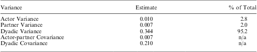
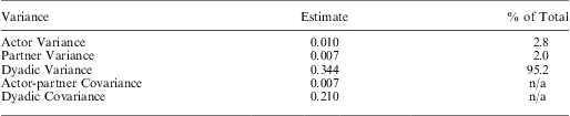
Next we examine the variances for the network of countries involved in MIDs during the 1952–2001 period (Table 2). It is clear that there is a lot of variance within this global network of countries, and it is even more apparent that the unique (dyadic) variance is much more salient than the individual actor or partner variance. If an analyst thought the salience of one dyad was independent of other dyads, then you would expect that the actor-partner and dyadic covariances would be essentially zero, but this is clearly not the case.
Variance Structure of Social Relations Model for 50 Years of MID Data
The sender and receiver (target) effects for both the network of total conflict onsets and an aggregated matrix of MID counts are shown in Figures 2 and 3, respectively. In each graphic, the countries are plotted from low to high, illustrating the exponential shape of the effects of individual countries on the overall pattern of militarized disputes since the end of World War II. We can see that incorporating counts of onsets in the matrix gives us a complete picture of conflict dynamics and the major players in this system. In the counts matrix, Russia and the United States top the list, followed by Iraq and China. Iran is close behind.
The actor (sender) effect of every country from a binary matrix representing the number of onsets of MIDs, 1952–2001
Note: these are sorted from low to high. Top actors are labeled.
The actor (sender) effect of every country from an aggregated matrix of counts representing the number of onsets of MIDs, 1952–2001
Note: these are sorted from low to high. Top actors are labeled.
In both matrices, the actors with the most impact are not the countries that would necessarily score the highest on conventional power metrics (though there is obviously some overlap). Not only can actor effects be negative (countries below the lower horizontal line), but the most salient countries in this domain have scores on actor effects that are two orders of magnitude larger than those at the median level of impact. Notably, the nodes with the most ties in Figure 10 (such as the United States, Iraq and Russia) place high in the actor effects plot in Figure 3. Similarly, we see that the United States and Russia rank highest on receiver (target) effects.
The basic point of this analysis is that by considering the dyadic interactions in the context of their interdependencies, a different picture emerges—one that reflects these dependencies as well as the independent power of countries to affect MIDs separately, both as actors and targets. If we turn to the analysis of how these actor and target effects vary over the same period, we see a more nuanced picture (shown in Figure 4). Here, we see that the sender (actor) effects and partner (target) effects vary substantially over time for the United States, Russia and China. Such figures clearly support the idea that the current approach to dyadic analysis in IR is incomplete and demonstrate how the SRM can reveal overlooked patterns in the data.
Individual actor effects for USA, Russia and China as both senders and targets over time
Scholars have long debated the role of reputation and repeated interactions in conditioning the ebb and flow of the international system. While directly addressing such questions is beyond the scope of this article, the results from the SRM shed light on the influence of major players in the international system in an easily interpretable and systematic way. To further this point, it is instructive to examine the actor effects of the United States and Russia over the most recent period. We present the unique relationship effects for the United States and Russia in Figures 5 and 6, respectively.
The evolution of US-Russia actor (sender) and target (receiver) effects, 1815–2001
Note: the red dots (in online version) and the corresponding arrows highlight the trajectory during the Second World War, while other years are shown in shades of gray. Darker shades indicate more recent years.
Dyadic, actor and target variance in the network of MIDs, 1816–2001
Figure 5 illustrates that Russia and the United States have actor effects that are largely independent of one another, and are not extraordinary in most years. The individual years from 1816 to 1938, and subsequent to 1945, are shown as gray dots with decreasing darkness as they recede in time (that is, the earliest years are the lightest, the most recent the darkest). Median levels are shown with thin rules, which transect the mass of points in the scatter plot. In 1939 an extraordinary cycle begins as the impact of Russia (the Soviet Union at this point in time) rises substantially until 1940. By 1941 the impact of the United States also jumps to a new level. Throughout WWII, these two actors have high levels of correlated impact on world politics, in terms of the conflict domain, but each declines rather quickly as the war draws to an end in 1945. By this point in time, each of the actor effects of Russia and the United States have returned to their pre-WWII averages, where they remain for the most part throughout the Cold War.Footnote 10 A similar correlation is seen in the pair's partner (target) effects as shown in Figure 5(b). Notably, target effects for 1940, 1943, 1944 and 1945 are quite similar.
Finally, we examine the dyadic versus the actor and target components of the network. The results shown in Figure 6 are produced by running the SRM on each matrix-year from 1816–2001. Here the dyadic variance in the SRM of militarized disputes is not only substantially larger than either the actor or target effects, but the movement of the variance over time has more variance. At major crisis points in the evolution of conflictual international relations we can see spikes in all three, but the dyadic variance has enormous spikes before the global wars, as well as during the 1960s and prior to the dismantling of the Soviet empire.
International Trade
The benefit of using the SRM is multilayered. First, we have shown that it directly models the dependencies in the data. However, such an approach can also then be used to compare multiple contexts of substantive interest. As a brief example, we compare the SRM results from 2000 trade data with the results generated by the MID data used in our study. Scholars have long theorized about the intersection of military might and economic prosperity as an indicator of global power; comparing such data using the SRM sheds light on the influence of those actors. Figure 7a shows the actor effects for data on the top 10 exporters in the year 2000; Figure 7b plots them against the actor effects generated for the same countries, in the same year, using the MID data.
Individual actor effects for top 10 exporters in 2000
Sources: IMF trade data and actor effects for the same states active in the MID dataset during the same year.
Next, we depart from the first half of our analysis and demonstrate how the SRM can be extended by incorporating covariates of interest. There are various approaches to incorporating covariates, such as structural equation modeling (Kenny, Kashy and Cook Reference Kenny, Kashy and Cook2006) and random effects ANOVA (Bond and Lashley Reference Bond and Lashley1996). These kinds of models can be estimated using MLwiN.Footnote 11 Hoff et al. (Reference Hoff, Fosdick, Volfovsky and Stovel2012) have also recently developed a wider range of techniques for nomination networks that also estimates the covariance structures within the SRM framework.Footnote 12 Another way this can be done is to estimate a latent space model, which integrates components of the basic SRM by incorporating the decomposition of variance into the error term of a bilinear mixed-effects model. This estimation also allows for a straightforward way to incorporate covariates specific to the actor, partner and dyadic relationships. In addition, the latent space model also builds on the SRM analysis by estimating third-order dependences (Hoff and Ward Reference Hoff and Ward2004).
Similar to second-order dependence, third-order dependence is commonly recognized in the social network analysis literature. Aspects of this higher-order dependence include transitivity, balance and clusterability (Wasserman and Faust Reference Wasserman and Faust1994).Footnote 13 An often-used example in the literature on third-order dependence considers the following relationships among a triad {i, j, k}. If we know that i considers j a friend and j is a friend of k, then the probability that k will also be a friend of i is likely to be higher than for a random person outside this triad, since i and k are at least indirectly connected in the friendship network by virtue of their separate linkages to j. In other words, knowing something about the relationships in the first two dyads in a triad often tells us something about the relations in the third dyad. As we think about the nature of the third-order dependence in some network datasets, a conceptualization of an ‘unobserved’ or latent ‘social space’ in which every network actor is embedded is very fruitful. Thus, for example, the observation of two links, i→j and j→k, suggests that i and k are not too far away from each other in this social space (which is often unobservable) and therefore are also likely to have a link between them.
Third-order dependence is an expression of the underlying probability of a link between two actors. We do not observe the complete set of all of these network characteristics, but we can infer them from the pattern of dyadic linkages. If we can map out the latent positions of each actor in the ‘social space,’ we can then assume that the ties in the network are conditionally independent. A series of latent models has been recently developed by Hoff, Raftery and Handcock (Reference Hoff, Raftery and Handcock2002) and Hoff (Reference Hoff2005) in which latent vectors, say ui and vj, for any two actors i and j are used to locate the actors in the ‘social space’ in order to account for third-order dependence. The latent model includes an estimate of the latent positions of each country in the investment network (ui and vj), which index the propensities for country pairs to have similar interaction patterns toward other countries. Put simply, if two countries share similar positions in the latent space, they have a higher probability of interacting with each other. This means a high level of bilateral transnational investment. The latent space model for dyadic data is based on an analysis of the actual dyadic matrices. A simple version of that model is given by the following specification:Footnote 14
 $${{y}_{i,j}} = \beta _{d}{\!\!'} {{x}_{i,j}}\, + \,\beta _{s}{\!\!'} {{x}_i}\, + \,\beta _{r}{\!\!'} {{x}_j}\, + \,{{a}_i}\, + \,{{b}_j}\, + \,{{\gamma }_{i,j}}\, + \,u_{i}{\!'} {{v}_j},$$
This implies the following moments for γi,j, which we estimate rather than ignore:
 $$E(\gamma _{{i,j}}^{{\rm{2}}} )\, = \,\sigma _{r}^{{\rm{2}}} \, + \,\sigma _{s}^{{\rm{2}}} \, + \,\sigma _{\gamma }^{{\rm{2}}} ;\; \; E({{\gamma }_{i,j}}{{{\epsilon}}_{j,i}})\, = \,\rho \sigma _{\gamma }^{{\rm{2}}} \, + \,{\rm{2}}{{\sigma }_{rs}};\; \; E({{\gamma }_{i,j}}{{{\epsilon}}_{i,k}})\, = \,\sigma _{r}^{{\rm{2}}} ;\; \; E({{\gamma }_{i,j}}{{{\epsilon}}_{k,j}})\, = \,\sigma _{s}^{{\rm{2}}} ;\; \; E({{\gamma }_{i,j}}{{{\epsilon}}_{k,i}})\, = \,{{\sigma }_{rs}},$$
where  $$$\sigma _{r}^{2} $$$
represents dependence among dyadic observations with a common partner,
 $$$\sigma _{s}^{2} $$$
represents dependence among measurements with a common sender and ρ represents the correlation of measurements within a dyad (that is, reciprocity). These dependencies are important.
This specification adds another layer to the SRM by configuring it to take clustering into account as well.Footnote 15 This model has been applied in a few places in political science (Ward, Siverson and Cao Reference Ward, Siverson and Cao2007; Ward and Hoff, Reference Ward and Hoff2007; Hoff and Ward Reference Hoff and Ward2004; Cao Reference Cao2009; Breunig, Cao and Luedtke Reference Breunig, Cao and Luedtke2012). It has also been extended to dynamic networks (Ward, Ahlquist and Rozenas Reference Ward, Ahlquist and Rozenas2013) and to dynamic networks combined with simple games (Metternich et al. Reference Metternich, Dorff, Gallop, Weschle and Ward2013). It has also been applied in a wide variety of studies outside the political science literature.Footnote 16
Figure 8 shows that the computationally simple SRM approach provides estimates of actor and partner effects that are fairly similar to the more elaborate estimation of a similar concept using the General Bilinear Effects Model. Though the scales are different, both approaches give very similar results for the individual effects of actors and partners in a small network of the top 10 exporters in 2000. The more elaborate approach is useful and captures some nuance that is not embedded in the SRM model. However, the basic answers for most networks will be close.
Actor and target effects generated by the GBME Versus SRM approach
Reciprocity and the Laws of War
In this section we apply the SRM and GBME to a long-standing question in IR: When do states follow the laws of war? We focus on the work by Morrow, who argues that institutional commitment shapes state behavior in following the laws of war (Morrow Reference Morrow2007). Namely, such commitments are established through three mechanisms: (1) treaties set the standard of expectations for wartime behavior, (2) states can reinforce agreements by responding to violations of treaties with similar actions and (3) the joint ratification of treaties strengthens their influence and therefore creates effective deterrence through reciprocity. In addition, ratification by democracies heightens compliance, whereas ratification loses its effect on non-democracies. The concept of reciprocity is key to Morrow's arguments. Indeed, he suggests that reciprocity is crucial not only for understanding behavior at the state level, but also for interpreting the behavior of individual soldiers on the battlefield. He analyzes the reciprocal nature of states in obeying the laws of war using dyadic data on compliance. To assess these claims, he employs an ordered probit modeling approach. In this section, we will discuss how the SRM and GBME provide leverage over other approaches, particularly by highlighting both the theoretical and methodological implications of reciprocity.
The data we will use is from Morrow and Jo (Reference Morrow and Jo2006), in which the authors record compliance with the laws of war for eight different ‘issue areas’ during 1900–92: the treatment of POWs, treatment of the wounded (enemy and civilian), respect for cultural property and general treatment of civilians. Compliance is conceptualized here using a 4-point ordinal scale in which the higher the value on the scale, the worse the violations against the laws of war (0 = no violations, 1 = infrequent/minor violations, 2 = frequent/major violations and 3 = the rules are completely disobeyed). The data is organized around each individual ‘warring dyad.’Footnote 17 To illustrate our point, we use one of the issue areas (treatment of POWs) and one time period within the data (1975–92), to create an n×n sociomatrix that best represents the dyadic nature of the data.Footnote 18
First, we use SRM on the sociomatrix for the selected time period. SRM allows us to analyze reciprocity at both the individual and dyadic levels. For example at the individual level, reciprocity is captured if actor i is hostile toward all others in the group, whether or not all others in the group are hostile toward actor i. In Figure 9 the sender and target effects are sorted from low to high; the correlation of these two effects expresses the general reciprocity between individual states. The generalized dyadic reciprocity has a covariance that is roughly equal to the unique variance (both about 0.33), while the actor and partner variances are minimal, as is the actor covariance (each approximately −0.01). These data are gleaned from calculating the basic quantities of the SRM, rather than asserting a priori the values of these quantities.
Sender and target effects for 1975–1992
Note: the correlation between sender and target effects = 0.94. The correlation between the two represents generalized reciprocity: the measure of how much a sender's actions influences the response of all of their partners.
For the dyadic level, we can assess whether partners within one dyad see each other as similar or interact with each other similarly. In general, we can say that for any dyadic pair, Xij, actor i's relationship effect toward actor j is correlated with actor j's relationship effect toward actor i. This measure closely gets at the dynamics Morrow discusses in his general theoretical framework for compliance. Namely, that compliance with the laws of war is a phenomenon that is largely driven by reciprocity: when one country mistreats POWs, the other is likely to do so as well. The SRM can demonstrate whether or not such dynamics are driving the patterns of the data. Figure 10 displays Morrow's original data on the left-hand side and a network of unique effects for the same set of countries. The right-hand side graph presents the 1975–92 network of states and highlights their dependent nature. Here the ties are weighted by the SRM unique effects for each dyad, with the highest unique effects shaded darkest (green in the online version). As we can see, clear patterns emerge; the dyadic pairs Iran-Iraq and Somalia-Ethiopia have the strongest unique effects, or reciprocal violations.
L: network graph of dyadic compliance from Morrow's data (1975–92); R: the network's unique effects
Note: the thinner gray (red in online version) lines indicate lower values of dyadic reciprocity while thicker, black (green in online version) ties indicate the highest values.
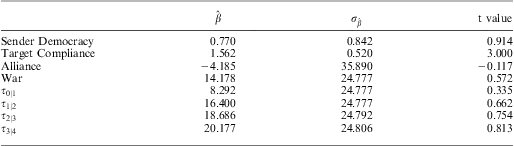
Lastly, we conclude with a comparison of the GBME approach to Morrow's ordered probit approach. Again we focus specifically on modeling the treatment of POWs during 1975–92. For the ordered probit replication, we include the most relevant variables from Morrow's study: the democracy score of the sender country, a binary variable that represents whether the countries in the dyad were in an alliance, a binary indicator of war and a compliance indicator for the target country using Morrow's 4-point ordinal scale (which, in his set-up, is used to measure reciprocity). In Table 3 we see that Morrow finds substantive support for the influence of democracy on compliance; democracy has a positive effect on the level of compliance for POW treatment. In his own words, “ratification by democracies, but not nondemocracies, correlates with greater compliance” (Morrow Reference Morrow2007). In addition, the ordered probit results seem to support the idea that the target state's compliance influences the compliance of the violating state. The GBME results, however, reveal a different story: when the network effects are taken into account, democracy plays no role in predicting compliance.
Ordered Probit Estimates for Treatment of POWs, 1975–92
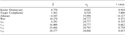
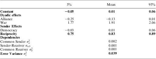
To replicate Morrow's study using our approach, we have to make some adjustments. His empirical analysis uses a variety of interaction terms that become numerically infeasible when one collapses a large number of years into a single analysis. The SRM and GBME work slightly differently, operating on an n×n sociomatrix. As mentioned, we use a smaller subset of the data than Morrow, and focus on the period from 1975–92. With a substantially smaller dataset to analyze, the nuanced and complicated interactions of Morrow's original analysis cannot be replicated exactly. Rather, we undertake an ‘in spirit’ replication. As we proceed, we include the democracy level of a country and whether or not the dyad is at war and whether the two countries are allied. These covariates are introduced into the GBME approach. The Bayesian analysis is run for 500,000 iterations, and every 100th is saved. As suggested by our SRM analysis, we find strong effects for reciprocity—much stronger than those in Morrow's model, as shown in Table 4.
Coefficient Estimates and Credible Intervals for Laws of War Analysis, 1975–1992
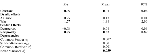
Our empirical results give some priority to network analysis over that which ignores interdependencies. As with our analysis of MIDs and trade, our results clearly demonstrate the utility of capturing the dependencies undergirding patterns of international relations. Specifically, our analysis of the laws of war suggests that democracy, as a covariate for the members of a network, has a weak effect, and this effect is imprecisely measured. Indeed, the effect for democracy is close to (and indistinguishable from) zero once the uncertainty of the estimation is taken into account. Importantly, we find that actual, measured reciprocity is very powerful and precisely estimated. In addition, alliances are shown not to be especially powerful but may be said to reduce compliance. The network measurement of this effect is much more precise than our simplistic replication of Morrow's work, but they both point in the same direction on the impacts of alliances. In general, although dependencies captured by the covariance terms are smaller than is typical of highly dependent networks, they are not small enough to ignore, and suggest that there is indeed a strong degree of second-order network clustering.
Though neither of the network approaches yields results that are overwhelming, the GBME reveals a more precise estimate of state compliance with the laws of war and highlights the dependencies discovered by the SRM analysis. Furthermore, both the GBME and SRM analyses emphasize reciprocity—measured by capturing dyadic effects—as a critical factor underlying our theoretical understanding of the laws of war. This contribution is significant. Our application of the SRM and GBME illustrates our central argument: that both theoretical and empirical research benefits from proper assessment and modeling of interdependent, dyadic data. Even in areas that have strong intuitions derived from carefully researched game theoretic approaches, it is critical to have a method of capturing the strategic interdependencies that embody the theoretical insights of such models.
Conclusion
On the whole, the field of IR has continually failed to take seriously the dependencies inherit in dyadic data. We argue that taking such a path is indefensible, and that there are simple alternatives. The SRM can serve as a straightforward tool for highlighting—instead of bypassing—such dependencies. We have demonstrated the nuanced analysis one can produce with the SRM, and have specifically shown its relevance for modeling dependencies in data on MIDs, trade and the laws of war.
The SRM approach to studying dyadic data has not been widely employed in political science, yet is widely used in psychology and sociology.Footnote 19 This approach holds great promise for political science projects that examine the influence of political actors on one another because it allows for a principled accounting of existing interdependencies among actors (and sets of actors) in the domain of politics, from the local to the international level. It allows one to estimate which actors are politically relevant without requiring ad hoc rules or ignoring available information. Because it has a framework similar to an ANOVA or regression framework, it is relatively easy to understand. It provides a precise way to attain unbiased estimates of all actor and partner effects, as well as dyadic relationship effects, in a given network. Known bias in estimators for data that are not properly considered independent and identically distributed can be eliminated. Furthermore, it is completely flexible to underlying distributions of data, embracing binomial, Poisson and Gaussian distributions. Perhaps most importantly, it gets us closer to modeling a plausible data-generating process that would create the kind of interdependent data we observe in international relations more broadly. The implementation of such a model is a major contribution to political science researchers who are motivated to accurately test theoretical claims about the international system.
APPENDIX A. SRM Replication Files and Program
For this project we have produced a statistical software to estimate the SRM model, which is available as an R script from the authors and the PSRM dataverse website. At the core of the R file is a function that enables the user to apply the SRM to any given square matrix. The data in the matrix can be binary, ordinal or continuous and either symmetric or non-symmetric. The input for the function is simply a square matrix, from which the function returns a list of SRM output: actor (sender) effects for each actor, partner (receiver) effects, dyadic effects, dyadic variance, actor variance, partner variance, actor-partner covariance and dyadic covariance. Additional functions allow the user to apply SRM to sociomatrices over time and plot specific SRM results over a given range.