2 Motivating examples

In this section we present various examples showing how our construction links different branches of mathematics. At this point, some of the equalities may seem numerically coincidental. However, as we will prove, these examples are instances of general theorems that work for arbitrary objects (graphs, linear systems of quadrics, linear concentration statistical models, determinantal hypersurfaces), irrespective of the choice made. In each example we use different fonts to indicate the numbers that are the same. Each case is based on a theorem from the next section. We hope that the examples exhibit how much information is provided in the polynomials ${\chi}_L$ and ${\chi}^{\prime }_L$ and with how many branches of mathematics they interact. In particular, the quite abstract Definition 3.3 of ${\chi}_L$ becomes better justified.

In the first example we show how our construction generalizes chromatic polynomials of arbitrary graphs. In order to make all of the objects as explicit as possible, we focus on the case when the graph G is the $6$ -cycle. The general theorem, applicable to arbitrary graphs, is stated in Corollary 3.14.

Example 2.1. The number of proper vertex colorings of an undirected graph G with k colors may be obtained as the value of a certain univariate polynomial ${\chi}_G(x)$ at $x=k$ , the chromatic polynomial. As long as G has at least one edge we have ${\chi}_G(1)=0$ , thus we define the reduced chromatic polynomial $\bar {{\chi}}(x):= {\chi}(x)/(x-1)$ .

Let us fix an arbitrary orientation of all edges of G. We assume that G is connected. We define the incidence matrix $A_G$ for the graph $G=(V,E)$ as the $|V|\times |E|$ matrix with columns labeled by edges E and rows labeled by vertices V, where $A_G(v,e)=1$ if v is the head of e, $A_G(v,e)=-1$ if v is the tail of e, and $0$ otherwise. The matrix $A_G$ defines a surjection from ${\mathbb {C}}^{|E|}$ to the codimension one subspace $C_0\subset {\mathbb {C}}^{|V|}$ defined by the condition that the coordinates sum up to zero. Equivalently, the transpose $A_G^t$ defines the injection $C_0^{\ast }\subset {\mathbb {C}}^{|E|}$ .

Let G be the $6$ -cycle. One can check [Reference Biggs12, Chapter 9] that we have

$$\begin{align*}{\chi}_G(x)=(x-1)^6+(x-1),\quad \bar{{\chi}}_G(x)=(x-1)^5+1=x^5-5x^4+\textit{10}x^3-10x^2+\mathbf{{5}}x.\end{align*}$$

For a suitable labeling and orientation of the edges, the incidence matrix is

$$\begin{align*}A_G= \begin{pmatrix} -1&1&0&0&0&0\\ 0&-1&1&0&0&0\\ 0&0&-1&1&0&0\\ 0&0&0&-1&1&0\\ 0&0&0&0&-1&1\\ 1&0&0&0&0&-1\\ \end{pmatrix}. \end{align*}$$

Our aim is to associate to G a linear subspace of diagonal matrices. The image of $A_G^t$ is the five-dimensional subspace $C_0^{\ast }\subset {\mathbb {C}}^{|E|}={\mathbb {C}}^6$ with coordinates summing up to zero. From now on we regard ${\mathbb {C}}^{|E|}$ as the space of $6\times 6$ diagonal matrices and $C_0^{\ast }$ as the subspace of diagonal matrices with trace zero.

Inverting all invertible matrices in $C_0^{\ast }$ and taking the closure, we obtain a hypersurface of diagonal matrices of degree $\mathbf {5}$ , defined by the fifth elementary symmetric polynomial in six variables. If we take a general subspace of codimension i (e.g., $i=2$ ) of $C_0^{\ast }$ , then the closure of the locus of inverses of invertible matrices in that space will be a variety of codimension $i+1$ of degree equal to the absolute value of the $(i+1)$ -st coefficient of $\bar {{\chi}}_G$ (e.g., $\textit {10}$ ). We have

$$\begin{align*}{\chi}_{C_0^{\ast}}(a,b)={\chi}_{C_0^{\ast}}'(a,b)= a^4 +5\cdot \binom{4}{1}a^3b +\textit{10}\cdot \binom{4}{2} a^2b^2 +10\cdot \binom{4}{3} ab^3 +\mathbf{5}\cdot b^4. \end{align*}$$

In the second example we show how our construction generalizes enumerative problems on quadrics. The general theorem is given in Proposition 3.17.

Example 2.2. Consider the eight-dimensional family of degree two polynomials in four variables $x_0,x_1,x_2,x_3$

(2.1) $$ \begin{align}\alpha x_0^2+\beta x_1^2+\gamma x_2^2+\delta x_3^2+2\epsilon x_0x_1+2\zeta x_1x_2+2\eta x_2x_3+2\theta x_3x_0,\end{align} $$

where $\alpha ,\beta ,\gamma ,\delta ,\epsilon ,\zeta ,\eta ,\theta $ are the parameters. Each (nonzero) member of this family defines a degree two hypersurface in ${\mathbb {P}}^3$ . Let us pick seven general hyperplanes in ${\mathbb {P}}^3$ . There are $\mathbf {{9}}$ smooth projective quadratic surfaces from the family (2.1) that are tangent to all the given hyperplanes.

The family in (2.1) may be identified with the space L of symmetric matrices given by

(2.2) $$ \begin{align} \begin{pmatrix} \alpha&\epsilon&0&\theta\\ \epsilon&\beta&\zeta&0\\ 0&\zeta&\gamma&\eta\\ \theta&0&\eta&\delta\\ \end{pmatrix}. \end{align} $$

Inverting all invertible matrices in that space and taking the closure of this set we obtain an affine algebraic variety of dimension eight and degree $\mathbf {{9}}$ . We have

$$ \begin{align*}{\chi}_L(a,b)&= \begin{aligned}[t] &a^7 +3\cdot \binom{7}{1} a^6 b +9\cdot \binom{7}{2} a^5 b^2 +17\cdot \binom{7}{3} a^4b^3 \\ &{}+21\cdot \binom{7}{4} a^3b^4 +21\cdot \binom{7}{5} a^2b^5 +17\cdot \binom{7}{6} ab^6 +\mathbf{9} b^7.\end{aligned} \end{align*} $$

In the third example we show how our construction is related to the maximum likelihood degree. The general theorem is given in Proposition 3.16.

Example 2.3. Let us consider the linear space L of concentration matrices given by

$$\begin{align*}A_{\alpha,\beta,\gamma,\delta,\epsilon}=\begin{pmatrix} \alpha&\beta&\delta\\ \beta&\gamma&\epsilon\\ \delta&\epsilon&\alpha+\beta+\gamma+\delta+\epsilon\\ \end{pmatrix}\,. \end{align*}$$

This means that we consider a family of probability distributions, each one being a multivariate Gaussian distribution on ${\mathbb {R}}^3$ , parameterized by those $\alpha ,\beta ,\gamma ,\delta ,\epsilon \in {\mathbb {R}}$ for which $A_{\alpha ,\beta ,\gamma ,\delta ,\epsilon }$ is positive definite and the mean $\mu \in {\mathbb {R}}^3$ . The associated probability distribution is

$$\begin{align*}f_{\alpha,\beta,\gamma,\delta,\epsilon,\mu}(x)=\frac{(\text{det} A_{\alpha,\beta,\gamma,\delta,\epsilon})^{\frac{1}{2}}}{(2\pi)^{\frac{3}{2}}}\exp{\left(-\frac{1}{2}(x-\mu)^TA_{\alpha,\beta,\gamma,\delta,\epsilon}(x-\mu)\right)}.\end{align*}$$

Such a family of probability distributions is called a statistical model. The one above is known as a linear concentration model [Reference Anderson13], as it is given by linear conditions on the concentration matrix. One of the aims of statistics is to fit the parameters (in our case $\alpha ,\beta ,\gamma ,\delta ,\epsilon ,\mu $ ) of the model, so that it best explains the given data. The data are a finite family of points $x_1,\dots , x_n\in {\mathbb {R}}^3$ . Estimating $\mu $ is easy, as one takes the mean of the data $x_i$ . For simplicity let us assume that $ \mu =0$ , which can always be achieved by shifting the data.

Our aim is to maximize the likelihood function in the parameters $\alpha ,\beta ,\gamma ,\delta ,\epsilon $ ,

$$\begin{align*}\prod_{i=1}^n f_{\alpha,\beta,\gamma,\delta,\epsilon,0}(x_i).\end{align*}$$

As the logarithm is monotonic, one considers the log-likelihood function

$$\begin{align*}\sum_{i=1}^n \log f_{\alpha,\beta,\gamma,\delta,\epsilon,0}(x_i),\end{align*}$$

which, up to a constant, equals

$$\begin{align*}\frac{n}{2}\log(\text{det} A_{\alpha,\beta,\gamma,\delta,\epsilon})-\frac{1}{2}\sum_{i=1}^n x_i^TA_{\alpha,\beta,\gamma,\delta,\epsilon}x_i.\end{align*}$$

First one computes the number of complex critical points of the function. By taking the partial derivatives, when the vector of the $x_i$ ’s is general and $n>3$ , we obtain 2 complex critical points. This number is known as the maximum likelihood degree, which in this case coincides with the degree of the model. Among the critical points, the maximum we look for will be the unique point for which $A_{\alpha ,\beta ,\gamma ,\delta ,\epsilon }$ is positive definite.

We may take the inverses of all invertible matrices in the space of symmetric matrices specified by the model. After taking the closure of this set, we obtain a variety of degree 2. We have

$$\begin{align*}{\chi}_L(a,b)={\chi}_L'(a,b)= a^4 +2\cdot \binom{4}{1}a^3b +4\cdot \binom{4}{2}a^2b^2 +4\cdot \binom{4}{3}ab^3 +\mathbf{2}\cdot b^4. \end{align*}$$

In the last example we show how our construction is related to the Euler characteristic of a determinantal hypersurface. The general theorem is given in Proposition 3.18.

Example 2.4. Consider the homogeneous cubic $f=(\alpha \gamma -\beta ^2)\delta $ in ${\mathbb {P}}^3$ . It defines a surface that consists of the plane $\delta =0$ (a ${\mathbb {P}}^2$ ) and the cone over a smooth conic in that plane, which is the image of ${\mathbb {P}}^1$ under the second Veronese embedding. The plane and the cone both intersect in the image of the second Veronese embedding of ${\mathbb {P}}^1$ . Thus, the Euler characteristic of the surface equals

$$\begin{align*}{\chi}(V(f))={\chi}({\mathbb{P}}^2)+1+{\chi}({\mathbb{P}}^1)-{\chi}({\mathbb{P}}^1)=4.\end{align*}$$

Hence, the complement of $V(f)$ in ${\mathbb {P}}^3$ has Euler characteristic equal to $\textbf {0}$ .

The cubic f is the determinant of the matrix

(2.3) $$ \begin{align} \begin{pmatrix} \alpha&\beta&0\\ \beta&\gamma&0\\ 0&0&\delta\\ \end{pmatrix}. \end{align} $$

Write L for the linear space of matrices of the form above. Inverting all invertible matrices in L and taking the closure, we obtain a variety of degree $m_0=1$ (i.e., a linear subspace). We may also first intersect L with one (resp. two, resp. three) general hyperplanes. Then, inverting all remaining invertible matrices and taking the closure we obtain a variety of degree $m_1=\textit {2}$ (resp. $m_2=2$ , resp. $m_3=1$ ). We have

$$\begin{align*}\sum_{k=0}^3 (-1)^k m_k=\mathbf{{0}}. \end{align*}$$

We have

$$\begin{align*}{\chi}_L(a,b)={\chi}_L'(a,b)= a^3 +2\cdot \binom{3}{1}a^2b +\textit{2}\cdot \binom{3}{2}ab^2 +b^3. \end{align*}$$

3 Main results

As in the introduction, let B and C be vector spaces of dimension n. We start by presenting two equivalent constructions of the variety of complete collineations ${\text{COL}}_n$ . For more information we refer the reader to [Reference Thaddeus10, Reference Dinu, Michałek and Seynnaeve14, Reference Massarenti15, Reference De Concini and Procesi11].

For $k=1,\dots , n-1$ let $D_k\subset {\mathbb {P}}(B\otimes C)$ be the projectivization of the locus of matrices of rank at most k in $B\otimes C$ . We may consider a sequence of blow-ups

$$\begin{align*}{\mathbb{P}}(B\otimes C)=: X_0\leftarrow X_1 \leftarrow\dots\leftarrow X_{n-2},\end{align*}$$

where in the k-th step we blow-up the strict transform of $D_k$ . We define the variety of complete collineations ${\text{COL}}_n$ to be $X_{n-2}$ .

More explicitly, for each $k = 1,\ldots ,n-1$ , there is a unique up to scale $\text{GL} (B)\times \text{GL} (C)$ -equivariant degree k polynomial map $m_k : B\otimes C \to \bigwedge ^k B\otimes \bigwedge ^k C$ obtained by the Veronese embedding $B\otimes C \to S^k(B\otimes C)$ followed by projection to the unique submodule $\bigwedge ^k B\otimes \bigwedge ^k C \subset S^k(B\otimes C)$ . In coordinates, this map extracts all $k\times k$ minors of its argument: Let $b_1,\ldots ,b_n$ and $c_1,\ldots ,c_n$ be bases of B and C, respectively. Then $m_k(\sum _{ij} M_{ij}b_i\otimes c_j) = \sum _{I,J} \text{det} (M_{I,J}) b_I \otimes c_J$ , where $I=\{i_1,\dots ,i_k\}$ and $J=\{j_1,\dots ,j_k\}$ range over size k subsets of $\{1,\ldots ,n\}$ , $M_{I,J}$ denotes the $k\times k$ submatrix of $[M_{ij}]$ with rows in I and columns in J, and $b_I = b_{i_1}\wedge \cdots \wedge b_{i_k}$ and $c_J = c_{j_1}\wedge \cdots \wedge c_{j_k}$ . Projectivizing and taking all maps simultaneously, we obtain a rational map

$$\begin{align*}{\mathbb{P}}(B\otimes C)\dashrightarrow {\mathbb{P}}(B\otimes C)\times {\mathbb{P}}\big(\bigwedge^2B\otimes\bigwedge^2 C\big)\times\dots\times{\mathbb{P}}\big(\bigwedge^{n-1}B \otimes\bigwedge^{n-1} C\big).\end{align*}$$

The closure of the image of this map is ${\text{COL}}_n$ .

The second construction gives us natural projections $\pi _k:{\text{COL}}_n\rightarrow {\mathbb {P}}(\bigwedge ^kB \otimes \bigwedge ^k C)$ for $k=1,\dots , n-1$ . In the Picard group of ${\text{COL}}_n$ we obtain the classes $[H_k]$ as pullbacks $\pi _k^{\ast }({\mathcal {O}}(1))$ . Equivalently, the $H_k$ ’s, considered as Weil divisors, are pullbacks of hyperplanes. From now on we work in the vector space $\text{Pic}_{\mathbb {Q}}({\text{COL}}_n)$ . The classes $[H_k]$ form a basis of that vector space [Reference Massarenti15, Theorem 3.13].

Every element S of degree $\dim ({\text{COL}}_n)-k$ in the Chow ring of ${\text{COL}}_n$ gives a homogeneous polynomial $P_S$ of degree k on $\text{Pic}_{\mathbb {Q}}({\text{COL}}_n)$ defined by

$$\begin{align*}P_S(D):= SD^k\in H_0(\operatorname{\text{COL}}_n,{\mathbb{Q}})\simeq {\mathbb{Q}},\end{align*}$$

where the product is taken in the Chow ring with rational coefficients. The top degree part of the Chow ring, which is identified with $H_0({\text{COL}}_n,{\mathbb {Q}})$ , is isomorphic to ${\mathbb {Q}}$ via the degree function [Reference Fulton17, Definition 1.4], [Reference Eisenbud and Harris16, Proposition 1.21 and Appendix C.3.4].

Definition 3.3. Let $L\subset B\otimes C$ be a dimension $d+1$ subspace containing an element of rank at least $n-1$ . We define the degree d polynomial

$$\begin{align*}P_L(D):= S D^d \in H_0(\operatorname{\text{COL}}_n,{\mathbb{Q}})\simeq {\mathbb{Q}}\end{align*}$$

on $\text{Pic}_{\mathbb {Q}}({\text{COL}}_n)$ , where S is the class of the strict transform of ${\mathbb {P}}(L)$ under $\pi _1$ and the last isomorphism is given by taking the degree $\int _{{\text{COL}}_n}$ . Observe that the condition that L contains matrices of rank at least $n-1$ is needed so that the class S is well-defined.

In the basis $[H_k]$ , we have

$$\begin{align*}P_L\Big(\sum_{k=1}^{n-1} a_k [H_k]\Big):= \sum_{b_1+\dots+b_{n-1}=d}{\binom{d}{b_1,\dots,b_{n-1}}}S\prod_{k=1}^{n-1} [H_k]^{b_k}\prod_{k=1}^{n-1}a_k^{b_k}.\end{align*}$$

We call the coefficients $L(b_1,\dots , b_{n-1}):= S\prod _{k=1}^{n-1} [H_k]^{b_k}$ the characteristic numbers of the linear subspace L.

Remark 3.4. The group $\text{GL} (B)\times \text{GL} (C)$ acts on ${\text{COL}}_n$ , and, considered as Weil divisors, the set of representatives of $[H_k]$ is also preserved under this group. Consequently, $P_L$ is a $\text{GL} (B)\times \text{GL} (C)$ -invariant.

Restricting $P_L$ to the line through $[H_1]$ and $[H_{n-1}]$ we obtain the chromatic polynomial of L,

(3.1) $$ \begin{align} {\chi}_L(a,b) := P_L(a[H_1]+b[H_{n-1}])= \sum_{k=0}^d \binom{d}{k} S[H_1]^k [H_{n-1}]^{d-k} a^k b^{d-k}. \end{align} $$

We note that, by definition, the characteristic numbers are also the multidegree of the strict transform S of ${\mathbb {P}}(L)$ under the embedding

$$\begin{align*}S\subset \operatorname{\text{COL}}_n \subset {\mathbb{P}}(B\otimes C)\times {\mathbb{P}}\big(\bigwedge^2B\otimes\bigwedge^2 C\big)\times\dots\times{\mathbb{P}}\big(\bigwedge^{n-1}B \otimes\bigwedge^{n-1} C\big).\end{align*}$$

Corollary 3.9. Suppose L contains an element of rank n, and let $i:{\mathbb {P}}(B\otimes C)\dashrightarrow {\mathbb {P}}(C^{\ast }\otimes B^{\ast })$ be the rational map corresponding to matrix inversion, or equivalently, the gradient of the determinant. Let $\Gamma _L\subset {\mathbb {P}}(B\otimes C)\times {\mathbb {P}}(C^{\ast }\otimes B^{\ast })$ be the closure of the graph of i restricted to ${\mathbb {P}} (L)$ (i.e., the closure of the locus of pairs of matrices $([A],[A^{-1}])\in {\mathbb {P}}(B\otimes C)\times {\mathbb {P}}(C^{\ast }\otimes B^{\ast })$ where $A\in L$ is invertible).

Then

$$\begin{align*}{\chi}_L(a,b)= \sum_{k=0}^d \binom{d}{k} m_k a^k b^{d-k},\end{align*}$$

where $(m_0,\dots ,m_d)$ is the multidegree of $\Gamma _L$ .

We see that we obtain the chromatic polynomial of L by restricting the gradient of the determinant to ${\mathbb {P}}(L)$ and looking at the multidegree of the graph. There is a closely related, but not the same in general, construction where we take the gradient of the restriction of the determinant.

Definition 3.10. Let $L\subset B\otimes C$ . As discussed in Remark 3.1, there is a well defined map

$$\begin{align*}\nabla(\text{det}|_{L}) :{\mathbb{P}}(L)\dashrightarrow {\mathbb{P}}(L^{\ast}).\end{align*}$$

Let $(m_0',m_1',\dots ,m_d')$ be the multidegree of the closure of the graph of $\nabla (\text{det} |_{L})$ considered as the subvariety of ${\mathbb {P}}(L)\times {\mathbb {P}}(L^{\ast })$ .

We define the relative chromatic polynomial of L

$$\begin{align*}{\chi}^{\prime}_L(a,b):= \sum_{k=0}^d\binom{d}{k} m_k'a^k b^{d-k}.\end{align*}$$

Equivalently, $\nabla (\text{det} |_{L})$ may be defined as a composition of the inclusion ${\mathbb {P}}(L)\subset {\mathbb {P}}(B\otimes C)$ with the gradient of the determinant and then with the projection ${\mathbb {P}}(B^{\ast }\otimes C^{\ast })\dashrightarrow {\mathbb {P}}(L^{\ast })$ from ${\mathbb {P}}(L^\perp )\subset {\mathbb {P}}(B^{\ast }\otimes C^{\ast })$ .

Lemma 3.11. Let h be a homogeneous polynomial on a vector space V. Let $L\subset V$ be a vector subspace not contained in the singular locus of $V(h)$ . Consider two maps

$$\begin{align*}\nabla h: {\mathbb{P}}(V)\dashrightarrow {\mathbb{P}}(V^{\ast}),\end{align*}$$

$$\begin{align*}\nabla (h_{|L}):{\mathbb{P}}(L)\dashrightarrow {\mathbb{P}}(L^{\ast})={\mathbb{P}}(V^{\ast}/L^\perp).\end{align*}$$

Suppose that the map $\nabla (h_{|L})$ is generically finite.

The multidegree of the graph of $\nabla h$ restricted to ${\mathbb {P}}(L)$ equals the multidegree of the graph of $\nabla (h_{|L})$ if and only if ${\mathbb {P}}(L^\perp )$ is disjoint from $\overline {\nabla h({\mathbb {P}}(L))}$ . If L is general, then this condition is satisfied.

Consider now the case that B and C have distinguished bases, That is, $B=C={\mathbb {C}}^n$ , and $L\subset {\mathbb {C}}^n \simeq {\text{Diag}}_n \subset {\mathbb {C}}^n \otimes {\mathbb {C}}^n$ consists of diagonal matrices. In this setting, matrix inversion becomes coordinatewise inversion and L is the data of a representable matroid on n points. By the more general results of Huh et al., the coefficients of ${\chi}_L'$ equal (up to binomial factors and alternating signs) the coefficients of the reduced chromatic polynomial of the associated matroid [Reference Huh1], and so do the coefficients of ${\chi}_L$ [Reference Huh and Katz2]. In particular, ${\chi}_L={\chi}_L'$ . As a direct proof is short and we find the fact very important, we present it below.

Corollary 3.13. Suppose $L\subset {\text{Diag}}_n\subset {\mathbb {C}}^n\otimes {\mathbb {C}}^n$ consists of diagonal matrices. Then

$$\begin{align*}{\mathbb{P}}(L^\perp)\cap \overline{\nabla\text{det} ({\mathbb{P}}(L))}=\emptyset\end{align*}$$

and hence ${\chi}_L={\chi}_L'$ .

Proof. Let $[a_1:\dots :a_n]\in {\mathbb {P}}(L^\perp )$ . Without loss of generality we may assume $a_1=1$ , $a_2\dots ,a_k\neq 0$ and $a_{k+1}=\dots =a_n=0$ . For contradiction let us assume that $[a_1:\dots :a_n]\in \overline {\nabla \text{det} ({\mathbb {P}}(L))}$ . This means that there exists a sequence of points indexed by j, $[b_{1,j}:\dots :b_{n,j}]\in {\mathbb {P}}(L)$ , such that

$$\begin{align*}[b_{1,j}^{-1}:\dots:b_{n,j}^{-1}]\rightarrow [a_1:\dots:a_n],\quad \text{as }j\rightarrow\infty.\end{align*}$$

In particular, by rescaling, we may assume $b_{1,j}=1$ , so $b_{i,j}\rightarrow a_i^{-1}$ for $i=1,\dots , k$ . Then

$$\begin{align*}0=\sum_{i=1}^k b_{i,j}a_{i}\rightarrow k,\end{align*}$$

which is a contradiction.

We next discuss why our setting of tensors, chromatic polynomials and characteristic numbers appears in different branches of mathematics, as shown in examples in Section 2. In the following, we will always define $d = \dim {\mathbb {P}}(L) = \dim L - 1$ .

By the results in [Reference Huh1, Reference Huh and Katz2] we obtain the following corollary, which explains Example 2.1.

Corollary 3.14. Let G be a connected graph (or more generally a representable matroid) with v vertices and e edges. Let $A_G$ be the incidence matrix of G. The row span of $A_G$ defines $L\subset {\mathbb {C}}^e \simeq {\text{Diag}}_e \subset {\mathbb {C}}^e\otimes {\mathbb {C}}^e$ , $\dim L = v - 1$ .

Then the reduced chromatic polynomial $\bar {{\chi}}_G(x)$ of G has degree $v-1$ , has constant term zero, and, for each $0\le k\le v-2$ ,

$$\begin{align*}\textstyle [(-1)^{v+k} x^{k+1} ] \bar{{\chi}}_G = L(v-2-k,0,\ldots,0,k) = [\binom {v-2}{k} a^{v-2-k} b^k] {\chi}_L = [\binom {v-2}{k} a^{v-2-k} b^k] {\chi}_L'. \end{align*}$$

In the above, we have written $[cx^k]p(x)$ for the coefficient of $cx^k$ in $p(x)$ , or equivalently, $\frac {1}{c}$ times the coefficient of $x^k$ in $p(x)$ .

Next, we provide relations to algebraic statistics, based on the results from [Reference Sturmfels and Uhler4, Reference Michałek, Monin and Wiśniewski5, Reference Manivel, Michałek, Monin, Seynnaeve and Vodička6]. This explains Example 2.3.

In the following proposition we explain why the characteristic numbers of tensors coincide with the characteristic numbers known in algebraic geometry. This is a very classical topic going back essentially to Schubert [Reference Schubert28].

Consider a linear system of quadrics ${\mathbb {P}}(L)\subset {\mathbb {P}}(S^2{\mathbb {C}}^n)$ . The classical characteristic number is the answer to the following enumerative problem: how many nondegenerate quadrics in ${\mathbb {P}}(L)$ pass through a general points and are tangent to b general hyperplanes? The following proposition explains Example 2.2.

The generalization of the above result to the case where we count the number of quadrics passing through $b_0$ points, tangent to $b_1$ lines, $b_2$ planes, $\dots $ , $b_{n-1}$ hyperplanes, given by $L(b_0,\dots , b_{n-1})$ , is straightforward.

Finally, using results from [Reference Huh1] and [Reference Dimca and Papadima7], we show how the relative chromatic polynomial is related to Euler characteristic of the determinantal locus. This explains Example 2.4.

Proposition 3.18. Let $L\subset B\otimes C$ be a linear subspace and let $X={\mathbb {P}}(L)\cap V(\text{det} )$ . Let ${\chi}_L'(a,b)= \sum _{k=0}^d\binom {d}{k} m_ka^k b^{d-k}$ . Then the Euler characteristic ${\chi}(X)$ of X equals

$$\begin{align*}\dim L-\sum_{k=0}^d (-1)^k m_k\end{align*}$$

and equivalently the Euler characteristic of the complement ${\chi}({\mathbb {P}}(L)\setminus X)$ equals

$$\begin{align*}\sum_{k=0}^d (-1)^k m_k.\end{align*}$$

4 Relation to tensor rank

Let us recall a classical $\text{GL} (A)\times \text{GL} (B)\times \text{GL} (C)$ invariant of tensors in $A\otimes B\otimes C$ , the rank, defined as the smallest r so that T may be written as a sum of r rank one tensors. The famous problem of determining the exponent of matrix multiplication was shown by Strassen to be equivalent to determining the asymptotics of the rank of the structure tensor of the matrix multiplication operator [Reference Strassen29, Reference Landsberg30]. For matrices, tensor rank is the familiar notion of matrix rank, which may be efficiently computed with well-known algorithms. For tensors of three places or more, however, determining rank is a difficult problem for which no efficient algorithm exists. Results for specific tensors often involve establishing upper and lower bounds. For instance, the structure tensor of $3\times 3$ matrix multiplication, a tensor in ${\mathbb {C}}^9\otimes {\mathbb {C}}^9\otimes {\mathbb {C}}^9$ , is known to have rank at least $19$ and at most $23$ [Reference Bläser31, Reference Laderman32].

In view of Remark 3.5, we may consider characteristic numbers and chromatic polynomials to be invariants of tensors. Since these invariants are potentially easier to determine than tensor rank, it is useful to understand any relation. One such relation arises in view of Proposition 4.3 below, which implies that characteristic numbers are semicontinuous, that is, they cannot increase under degeneration. Unlike for matrices, the set of tensors of rank at most r is not closed. There is, correspondingly, a notion of border rank of a tensor, the smallest r so that the tensor is a degeneration of tensors of rank r. In particular, since any tensor of border rank r is a degeneration of general tensors of rank r, if a tensor has a characteristic number larger than that of a general tensor of rank r, then it must have border rank strictly larger than r.

We compute the chromatic polynomials of general tensors $T_{\text {gen},d,n,r}$ of rank r in $A \otimes B\otimes C$ , $\dim A = d+1$ , $\dim B = \dim C = n$ , for small values of d, n, and r. Such tensors correspond to dimension $d+1$ linear subspaces $L_{\text {gen},d,n,r}\subset B\otimes C$ contained in the span of r rank one elements of $B\otimes C$ and are general with respect to this property. By $L_{\text {gen},d,n,r}(b_1,\ldots ,b_{n-1})$ we mean the characteristic number of the subspace associated to $T_{\text {gen},d,n,r}$ . However, there is significant redundancy in these numbers; specifically, a general linear restriction of a general tensor of rank r is still a general tensor of rank r, so we have

$$\begin{align*}L_{\text{gen},d+k,n,r}(k,0,\ldots,0,d) = L_{\text{gen},d,n,r}(0,\ldots,0,d). \end{align*}$$

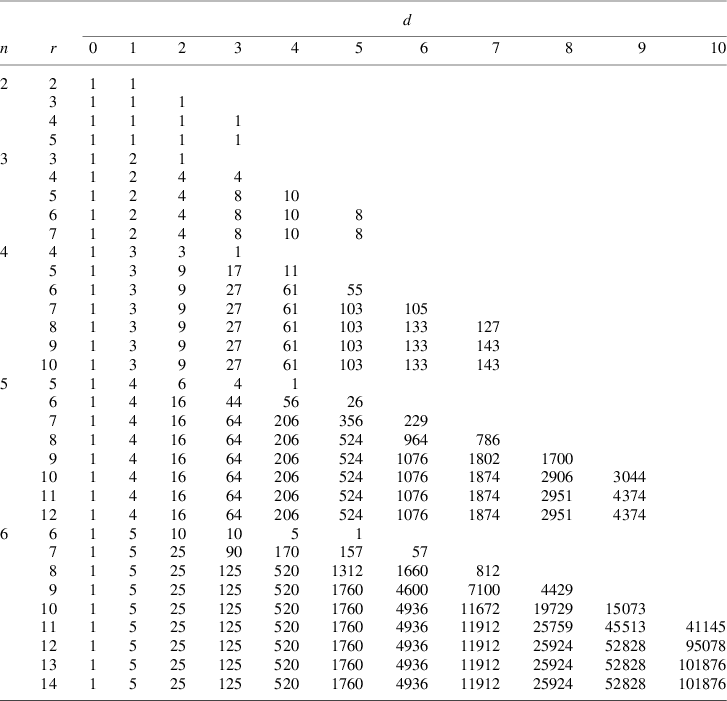
Hence, we only need to give the numbers $b_{d,n,r}= L_{\text {gen},d,n,r}(0,\ldots ,0,d)$ in order to describe all such chromatic polynomials. These values are presented in Table 1 for n up to $6$ .

Table 1

Values for $b_{d,n,r}$ .

Table 1 Long description

The table is organized with columns for n, r, and d (ranging from 0 to 10).

* For n equals 2:

- r equals 2: d values are 1, 1.

- r equals 3: d values are 1, 1, 1.

- r equals 4: d values are 1, 1, 1, 1.

- r equals 5: d values are 1, 1, 1, 1.

* For n equals 3:

- r equals 3: d values are 1, 2, 1.

- r equals 4: d values are 1, 2, 4, 4.

- r equals 5: d values are 1, 2, 4, 8, 10.

- r equals 6: d values are 1, 2, 4, 8, 10, 8.

- r equals 7: d values are 1, 2, 4, 8, 10, 8.

* For n equals 4:

- r equals 4: d values are 1, 3, 3, 1.

- r equals 5: d values are 1, 3, 9, 17, 11.

- r equals 6: d values are 1, 3, 9, 27, 61, 55.

- r equals 7: d values are 1, 3, 9, 27, 61, 103, 105.

- r equals 8: d values are 1, 3, 9, 27, 61, 103, 133, 127.

- r equals 9: d values are 1, 3, 9, 27, 61, 103, 133, 143.

- r equals 10: d values are 1, 3, 9, 27, 61, 103, 133, 143.

* For n equals 5:

- r equals 5: d values are 1, 4, 6, 4, 1.

- r equals 6: d values are 1, 4, 16, 44, 56, 26.

- r equals 7: d values are 1, 4, 16, 64, 206, 356, 229.

- r equals 8: d values are 1, 4, 16, 64, 206, 524, 964, 786.

- r equals 9: d values are 1, 4, 16, 64, 206, 524, 1076, 1802, 1700.

- r equals 10: d values are 1, 4, 16, 64, 206, 524, 1076, 1874, 2906, 3044.

- r equals 11: d values are 1, 4, 16, 64, 206, 524, 1076, 1874, 2951, 4374.

- r equals 12: d values are 1, 4, 16, 64, 206, 524, 1076, 1874, 2951, 4374.

* For n equals 6:

- r equals 6: d values are 1, 5, 10, 10, 5, 1.

- r equals 7: d values are 1, 5, 25, 90, 170, 157, 57.

- r equals 8: d values are 1, 5, 25, 125, 520, 1312, 1660, 812.

- r equals 9: d values are 1, 5, 25, 125, 520, 1760, 4600, 7100, 4429.

- r equals 10: d values are 1, 5, 25, 125, 520, 1760, 4936, 11672, 19729, 15073.

- r equals 11: d values are 1, 5, 25, 125, 520, 1760, 4936, 11912, 25759, 45513, 41145.

- r equals 12: d values are 1, 5, 25, 125, 520, 1760, 4936, 11912, 25924, 52828, 95078.

- r equals 13: d values are 1, 5, 25, 125, 520, 1760, 4936, 11912, 25924, 52828, 101876.

- r equals 14: d values are 1, 5, 25, 125, 520, 1760, 4936, 11912, 25924, 52828, 101876.

In view of Proposition 3.8, characteristic numbers and coefficients of the chromatic polynomial can be obtained by counting solutions to a sufficiently general polynomial system. This can be done in practice in two conceptually distinct ways, either symbolically or numerically. In this article, the numerical method of homotopy continuation, as implemented in the HomotopyContinuation.jl Julia library [Reference Breiding and Timme33], was used to count solutions. The code may be obtained at https://github.com/adconner/CharacteristicNumbers.jl.

Remark 4.1. As a subspace of matrices $L\subset B\otimes C$ moves to a special position, the pullback of ${\mathbb {P}}(L)$ to the variety of complete collineations breaks into several components. One of them is the strict transform. The other components have nonnegative contributions to the intersection product as they are intersected with basepoint free divisors. Thus special subspaces L give us smaller (or equal) characteristic numbers than general ones; a formal proof is presented below. For general L (thus for general tensors) we have explicit methods to compute the characteristic numbers [Reference Manivel, Michałek, Monin, Seynnaeve and Vodička6]. This means that if we take a general tensor of high enough rank r, we know $b_{d,n,r}=: b_{d,n}$ . For example,

$$\begin{align*}b_{2,3}=4,b_{3,4}=27,b_{4,5}=206,b_{5,6}=1760,b_{6,7}=16472,b_{7,8}=168007,b_{8,9}=1866790.\end{align*}$$

However, for small r the number $b_{d,n,r}$ will be smaller. It is very interesting to see when the transition happens. Our numerical results show that, for $d=n-1$ and $n=3,4,5,6,7,8$ , these are, respectively, $r=4,6,7,9,11,13$ .

The characteristic numbers of special tensors can also be computed using theoretical methods. One of the recent successful applications was a proof of a conjecture by Sturmfels and Uhler [Reference Sturmfels and Uhler4, Conjecture 2] given in [Reference Dinu, Michałek and Vodička34]. This shows that it is possible to provide explicit examples of tensors for which the characteristic numbers grow exponentially with respect to the dimension.

The proposition below shows that the coefficients of the chromatic polynomial are semicontinuous in the space of tensors, that is, in an irreducible subvariety of a tensor space, the coefficients of the chromatic polynomial are constant for generic points of the variety and decrease for nongeneric tensors.

Slightly more generally we obtain the following.

Proof. Let $\tilde \gamma $ be the open set of smooth points of $\gamma $ . Consider a constructible set $X\subset \tilde \gamma \times {\mathbb {P}}(B\otimes C)\times {\mathbb {P}}\big (\bigwedge ^2 B\otimes \bigwedge ^2 C \big )\times \dots \times {\mathbb {P}}\big (\bigwedge ^{n-1} B \otimes \bigwedge ^{n-1} C\big )$ given by tuples $(c',M_1,\dots , M_{n-1})$ , where $M_1$ is a full rank matrix in the space represented by $c'\in \tilde \gamma \subset G(d+1,B\otimes C)$ and $M_k$ is a matrix obtained by taking all $k\times k$ minors of $M_1$ . Let $\overline X$ be the closure of X. Note that X and $\overline X$ are irreducible.

The general fiber of the projection $f:\overline X \rightarrow \tilde \gamma $ over $c'\in \tilde \gamma $ coincides with the strict transform $S_{c'}\subset {\text{COL}}_n$ of the space ${\mathbb {P}}(L_{c'})$ corresponding to $c'$ . By [Reference Hartshorne19, Proposition 9.7], the map $\overline X\rightarrow \tilde \gamma $ is flat, and thus each fiber provides the same class in the Chow ring of $\overline X$ . Now the fiber over $c\in \tilde \gamma \subset \gamma $ may have several components but one of them must be $S_c$ , the strict transform of ${\mathbb {P}}(L_c)$ . If we let the components be $Y_1=S_c, Y_2,\dots , Y_N$ , we obtain:

$$\begin{align*}\text{deg} \left([S_{c'}]\prod_{k=1}^{n-1} [H_k]^{b_k}\right)=\text{deg} \left(([S_c]+[Y_2]+\dots+[Y_N])\prod_{k=1}^{n-1} [H_k]^{b_k}\right)\geq \text{deg} \left([S_c]\prod_{k=1}^{n-1} [H_k]^{b_k}\right),\end{align*}$$

where the last inequality follows from the fact that $[H_k]$ ’s are base point free and $[Y_j]$ ’s are effective.