1 Introduction
In oceans and lakes, interactions between surface waves and wind-driven currents can induce Langmuir cells (LCs) in the pattern of counter-rotating streamwise-elongated vortex pairs (see e.g. Langmuir Reference Langmuir1938; Scott et al. Reference Scott, Myer, Stewart and Walther1969; Craik & Leibovich Reference Craik and Leibovich1976; Weller & Price Reference Weller and Price1988; Smith Reference Smith1992; Thorpe Reference Thorpe1992; Farmer & Li Reference Farmer and Li1995; Skyllingstad & Denbo Reference Skyllingstad and Denbo1995; McWilliams, Sullivan & Moeng Reference McWilliams, Sullivan and Moeng1997). The LCs can significantly impact the transport of mass, momentum and heat (Leibovich Reference Leibovich1983; Smith Reference Smith2001; Thorpe Reference Thorpe2004; Sullivan & McWilliams Reference Sullivan and McWilliams2010; D’Asaro Reference D’Asaro2014), and therefore influence the climate (Belcher et al. Reference Belcher, Grant, Hanley, Fox-Kemper, Van-Roekel, Sullivan, Large, Brown, Hines and Calvert2011) and ecology (Barstow Reference Barstow1983) in oceans and lakes. The LCs and the residual small-scale background turbulence in Langmuir turbulence constitute a multi-scale system. The investigations on LCs and their effects on background turbulence are important for the development of ocean models.
In shallow waters, LCs can engulf the entire water column and induce large-scale momentum flux (Gargett et al. Reference Gargett, Wells, Tejada-Martínez and Grosch2004; Dethleff & Kempema Reference Dethleff and Kempema2007; Gargett & Wells Reference Gargett and Wells2007; Tejada-Martínez & Grosch Reference Tejada-Martínez and Grosch2007; Dierssen et al. Reference Dierssen, Zimmerman, Drake and Burdige2009; Kukulka, Plueddemann & Sullivan Reference Kukulka, Plueddemann and Sullivan2012; Akan et al. Reference Akan, Tejada-Martínez, Grosch and Martinat2013; Savidge & Gargett Reference Savidge and Gargett2017). In the field, Gargett et al. (Reference Gargett, Wells, Tejada-Martínez and Grosch2004) and Gargett & Wells (Reference Gargett and Wells2007) observed LCs in neutrally stratified shallow waters, and then measured the velocity fluctuations and studied the characteristics of the LCs. Based on the Craik–Leibovich (CL) equations (Craik & Leibovich Reference Craik and Leibovich1976; Leibovich Reference Leibovich1977), Tejada-Martínez & Grosch (Reference Tejada-Martínez and Grosch2007) conducted large-eddy simulations (LES) of shallow-water Langmuir turbulence. The spanwise length scale of the LCs, the mean velocity profile and the Lumley invariant map obtained from LES (Tejada-Martínez & Grosch Reference Tejada-Martínez and Grosch2007) are in good agreement with the field measurement (Gargett & Wells Reference Gargett and Wells2007). In the subsequent works, experimental and LES studies were conducted to investigate shallow-water Langmuir turbulence under different environmental conditions that involve the Coriolis force (Grosch & Gargett Reference Grosch and Gargett2016), surface heat flux (Gargett & Grosch Reference Gargett and Grosch2014; Gargett, Savidge & Wells Reference Gargett, Savidge and Wells2014; Walker, Tejada-Martínez & Grosch Reference Walker, Tejada-Martínez and Grosch2016), tidal currents (Kukulka et al. Reference Kukulka, Plueddemann, Trowbridge and Sullivan2011; Martinat et al. Reference Martinat, Xu, Grosch and Tejada-Martínez2011; Shrestha, Anderson & Kuehl Reference Shrestha, Anderson and Kuehl2018) and wave breaking (Gerbi et al. Reference Gerbi, Trowbridge, Terray, Plueddemann and Kukulka2009; Li et al. Reference Li, Li, Gerbi and Song2013).
In neutrally stratified shallow waters, LCs impose significant impacts on turbulence statistics throughout the water column. The logarithmic layers near the water bottom and water surface are disrupted due to the vertical momentum flux induced by the LCs (Tejada-Martínez et al. Reference Tejada-Martínez, Grosch, Sinha, Akan and Martinat2012, Reference Tejada-Martínez, Akan, Sinha, Grosch and Martinat2013; Sinha et al. Reference Sinha, Tejada-Martínez, Akan and Grosch2015; Deng et al. Reference Deng, Yang, Xuan and Shen2019). The LCs also alter the intensity of velocity fluctuations (Tejada-Martínez & Grosch Reference Tejada-Martínez and Grosch2007; Tejada-Martínez et al. Reference Tejada-Martínez, Grosch, Sinha, Akan and Martinat2012; Martinat, Grosch & Gatski Reference Martinat, Grosch and Gatski2014; Sinha et al. Reference Sinha, Tejada-Martínez, Akan and Grosch2015; Deng et al. Reference Deng, Yang, Xuan and Shen2019). Owing to the contributions of the LCs, the spanwise velocity fluctuations are enhanced near the water bottom and surface, while the vertical velocity fluctuations become stronger in the central region of the water column (Tejada-Martínez & Grosch Reference Tejada-Martínez and Grosch2007; Martinat et al. Reference Martinat, Grosch and Gatski2014; Sinha et al. Reference Sinha, Tejada-Martínez, Akan and Grosch2015; Deng et al. Reference Deng, Yang, Xuan and Shen2019). At high Reynolds numbers, LCs induce an additional outer peak in the profile of the streamwise Reynolds normal stress (Deng et al. Reference Deng, Yang, Xuan and Shen2019).
While LCs can induce large-scale mixing of momentum and scalars, the contribution of the background turbulence at smaller scales is also important in shallow-water Langmuir turbulence (Kukulka et al. Reference Kukulka, Plueddemann and Sullivan2012; Martinat et al. Reference Martinat, Grosch and Gatski2014; Sinha et al. Reference Sinha, Tejada-Martínez, Akan and Grosch2015; Deng et al. Reference Deng, Yang, Xuan and Shen2019). The magnitudes of the Reynolds stresses of the background turbulence are comparable to those of the LC content in the central region of the water column and are even larger near the bottom and surface (Martinat et al. Reference Martinat, Grosch and Gatski2014; Sinha et al. Reference Sinha, Tejada-Martínez, Akan and Grosch2015; Deng et al. Reference Deng, Yang, Xuan and Shen2019). As pointed out by Akan et al. (Reference Akan, Tejada-Martínez, Grosch and Martinat2013) and Sinha et al. (Reference Sinha, Tejada-Martínez, Akan and Grosch2015), the intensity of the vertical velocity in the background turbulence is significantly enhanced near the water surface due to the Stokes drift of surface waves, and, as a result, the background turbulence is more important than LCs in the transport of mass and heat across the water surface (Gemmrich & Farmer Reference Gemmrich and Farmer1999; Akan et al. Reference Akan, Tejada-Martínez, Grosch and Martinat2013; Takagaki et al. Reference Takagaki, Kurose, Tsujimoto, Komori and Takahashi2015).
It was reported in the literature that, in other wall-bounded turbulent flows with large-scale structures, the intensity of the residual background turbulence is significantly modulated by the large-scale structures (Hutchins & Marusic Reference Hutchins and Marusic2007; Mathis, Hutchins & Marusic Reference Mathis, Hutchins and Marusic2009; Anderson Reference Anderson2016; Dai, Huang & Xu Reference Dai, Huang and Xu2016; Deng, Huang & Xu Reference Deng, Huang and Xu2016; Salesky & Anderson Reference Salesky and Anderson2018). Specifically, in the high-Reynolds-number turbulent boundary layer, the near-wall background turbulence is locally enhanced and suppressed in the regions with high-speed and low-speed large-scale motions, respectively (Hutchins & Marusic Reference Hutchins and Marusic2007; Mathis et al. Reference Mathis, Hutchins and Marusic2009). This finding inspired the development of new turbulence models. For example, new wall-layer models were developed to account for the localizing effect of large-scale structures on the background turbulence, which improved the performance of LES in predicting near-wall turbulence statistics (Inoue et al. Reference Inoue, Mathis, Marusic and Pullin2012; Howland & Yang Reference Howland and Yang2018; Yin, Huang & Xu Reference Yin, Huang and Xu2018).
Compared with the large-scale structures in turbulent boundary layers, LCs are more organized and energetic (Tejada-Martínez & Grosch Reference Tejada-Martínez and Grosch2007; Deng et al. Reference Deng, Yang, Xuan and Shen2019), and therefore are expected to impose a more significant localizing effect on the background turbulence. In the investigation of scalar transport near the sea surface, Akan et al. (Reference Akan, Tejada-Martínez, Grosch and Martinat2013) observed that streaks consisting of large-magnitude streamwise velocity of background turbulence are concentrated above the downwelling limbs of LCs, where the streamwise velocity of the LC content is positive. Takagaki et al. (Reference Takagaki, Kurose, Tsujimoto, Komori and Takahashi2015) noted that the small-scale vortices are intensified in the surface convergent regions with positive streamwise velocity of the LC content. The findings of Akan et al. (Reference Akan, Tejada-Martínez, Grosch and Martinat2013) and Takagaki et al. (Reference Takagaki, Kurose, Tsujimoto, Komori and Takahashi2015) explain the observation in the field that small windrows occur at the two flanks of the main windrows to form a ‘Y’-junction pattern (Langmuir Reference Langmuir1938; Scott et al. Reference Scott, Myer, Stewart and Walther1969; Assaf, Gerard & Gordon Reference Assaf, Gerard and Gordon1971; Weller & Price Reference Weller and Price1988; Thorpe Reference Thorpe1992; Farmer & Li Reference Farmer and Li1995). Martinat et al. (Reference Martinat, Grosch and Gatski2014) observed that the statistics of background turbulence averaged over time and the horizontal plane are different from those without applying the spanwise averaging. This observation indicates that the intensities of background turbulence vary with the spanwise location. Martinat et al. (Reference Martinat, Grosch and Gatski2014) further stressed that the localizing effect of LCs on the background turbulence needs to be considered in the Reynolds-averaged Navier–Stokes (RANS) simulation of Langmuir turbulence.
To date, the localizing effect of the LCs on the background turbulence has not been studied systematically. The following questions associated with the localizing effect need to be answered:
(1) Is the localizing effect of the LCs on the background turbulence in the bottom boundary layer similar to that in the surface boundary layer?
(2) What is the underlying mechanism for the localizing effect?
(3) How does one develop models that predict the localized turbulence intensity or momentum flux of the background turbulence?
To answer the above questions, in this study we further analyse the LES database of shallow-water Langmuir turbulence obtained by Deng et al. (Reference Deng, Yang, Xuan and Shen2019). The LCs and background turbulence are quantified based on a triple decomposition of the flow field, and the localized Reynolds stresses are defined as the time and streamwise average of the second moments of the background turbulence velocity fluctuations. A comparison of the localized Reynolds stresses at different spanwise locations shows the localizing effects quantitatively. The transport equations of the localized Reynolds stresses are derived, and the dominant sources in the budget balance of the localized Reynolds stresses are analysed to reveal the mechanisms underlying the localizing effect, based on which predictive models are proposed to scale the localized Reynolds stresses.
The remainder of this paper is organized as follows. The simulation method and computational cases are introduced in § 2. In § 3, how the intensities of the background turbulence vary in the spanwise direction is revealed. In § 4, the key mechanisms underlying the localizing effect are studied through the analyses of the budget terms in the transport equations of the localized Reynolds stresses. In § 5, predictive models of the localized Reynolds stresses are proposed based on the key mechanisms found in § 4 to assess the spatial dependence of Boussinesq-model parameters in shallow-water Langmuir turbulence for the localized Reynolds stresses. The localizing effects at a practical Reynolds number are further discussed in § 6. Finally, our main conclusions are given in § 7.
2 Simulation method and computational cases
2.1 Governing equations
The localizing effects of LCs on the background turbulence are mainly studied through the analyses of the database obtained from the wall-resolved LES (Deng et al. Reference Deng, Yang, Xuan and Shen2019) and wall-modelled LES of neutrally stratified shallow-water Langmuir turbulence. The following continuity and CL equations (McWilliams et al. Reference McWilliams, Sullivan and Moeng1997; Tejada-Martínez & Grosch Reference Tejada-Martínez and Grosch2007) were simulated:
 $$\begin{eqnarray}\displaystyle & \displaystyle \frac{\unicode[STIX]{x2202}\overline{u}_{i}}{\unicode[STIX]{x2202}x_{i}}=0, & \displaystyle\end{eqnarray}$$
 $$\begin{eqnarray}\displaystyle & \displaystyle \frac{\unicode[STIX]{x2202}\overline{u}_{i}}{\unicode[STIX]{x2202}t}+\overline{u}_{j}\frac{\unicode[STIX]{x2202}\overline{u}_{i}}{\unicode[STIX]{x2202}x_{j}}=-\frac{1}{\unicode[STIX]{x1D70C}}\frac{\unicode[STIX]{x2202}\overline{\unicode[STIX]{x1D6F1}}}{\unicode[STIX]{x2202}x_{i}}+\unicode[STIX]{x1D708}\frac{\unicode[STIX]{x2202}^{2}\overline{u}_{i}}{\unicode[STIX]{x2202}{x_{j}}^{2}}+\unicode[STIX]{x1D716}_{ijk}u_{j}^{S}\overline{\unicode[STIX]{x1D714}}_{k}+\frac{\unicode[STIX]{x2202}\unicode[STIX]{x1D70F}_{ij}^{sgs}}{\unicode[STIX]{x2202}x_{j}}. & \displaystyle\end{eqnarray}$$
The coordinates  $x_{1}$,
 $x_{2}$ and
 $x_{3}$ (or
 $x$,
 $y$ and
 $z$) denote the streamwise, vertical and spanwise directions, respectively, with
 $\overline{u}_{1}$,
 $\overline{u}_{2}$ and
 $\overline{u}_{3}$ (or
 $\overline{u}$,
 $\overline{v}$ and
 $\overline{w}$) representing the corresponding velocity components. The overline stands for the implicit grid-level filter in LES. The effective pressure
 $\overline{\unicode[STIX]{x1D6F1}}$ is the summation of the resolved pressure
 $\overline{p}$ and an additional part
 $\overline{\unicode[STIX]{x1D6E4}}$ defined as (McWilliams et al. Reference McWilliams, Sullivan and Moeng1997)
 $$\begin{eqnarray}\overline{\unicode[STIX]{x1D6E4}}=0.5u_{j}^{S}u_{j}^{S}+u_{j}^{S}\overline{u}_{j}.\end{eqnarray}$$
The third term on the right-hand side of (2.2) is the CL vortex forcing term, where  $\unicode[STIX]{x1D716}_{ijk}$ is the third-order Levi-Civita symbol,
 $\overline{\unicode[STIX]{x1D714}}_{i}=\unicode[STIX]{x1D716}_{ijk}\unicode[STIX]{x2202}\overline{u}_{k}/\unicode[STIX]{x2202}x_{j}$ is the resolved vorticity and
 $u_{i}^{S}$ is the Stokes drift velocity induced by the water wave. In shallow water,
 $u_{i}^{S}$ is given as (Tejada-Martínez & Grosch Reference Tejada-Martínez and Grosch2007)
 $$\begin{eqnarray}u_{1}^{S}=u^{S\ast }\frac{\cosh (2ky)}{2\sinh ^{2}(2kh)}=\frac{u_{\unicode[STIX]{x1D70F}}}{La_{t}^{2}}\frac{\cosh (2ky)}{2\sinh ^{2}(2kh)},\quad u_{2}^{S}=u_{3}^{S}=0,\quad y\in [0,2h].\end{eqnarray}$$
Here,  $u^{S\ast }$ is the characteristic velocity of the Stokes drift of water waves in shallow water (Tejada-Martínez & Grosch Reference Tejada-Martínez and Grosch2007), which is defined as
 $u^{S\ast }=\unicode[STIX]{x1D70E}ka^{2}$, with
 $\unicode[STIX]{x1D70E}$,
 $k$ and
 $a$ being the frequency, wavenumber and wave amplitude, respectively. The water depth is
 $2h$. The surface friction velocity
 $u_{\unicode[STIX]{x1D70F}}$ equals
 $\sqrt{\unicode[STIX]{x1D70F}_{w}/\unicode[STIX]{x1D70C}}$, where
 $\unicode[STIX]{x1D70F}_{w}$ is the wind stress imposed on the surface and
 $\unicode[STIX]{x1D70C}$ is the density of water. The turbulent Langmuir number
 $La_{t}=\sqrt{u_{\unicode[STIX]{x1D70F}}/u^{S\ast }}$ characterizes the relative importance of the wind shear to the CL vortex force related to the Stokes drift of surface waves (McWilliams et al. Reference McWilliams, Sullivan and Moeng1997). From (2.2) and (2.4), it is understood that the magnitude of the CL vortex force decreases monotonically as the value of either
 $La_{t}$ or
 $kh$ increases. In the last term of (2.2),
 $\unicode[STIX]{x1D70F}_{ij}^{sgs}$ is the subgrid-scale (SGS) stress tensor, calculated using the dynamic Smagorinsky model (Smargorinsky Reference Smargorinsky1963; Germano et al. Reference Germano, Piomelli, Moin and Cabot1991; Lilly Reference Lilly1992).
Periodic boundary conditions are applied in the streamwise ( $x$) and spanwise (
 $z$) directions. At the water bottom (
 $y=0$), the no-slip boundary condition is imposed. In wall-resolved LES, the bottom boundary condition is
 $u=v=w=0$. In wall-modelled LES, the vertical velocity at the bottom is zero, and the streamwise and spanwise shear stresses at the bottom are calculated using the equilibrium-stress model (Balaras, Benocci & Piomelli Reference Balaras, Benocci and Piomelli1995; Pope Reference Pope2001; Piomelli & Balaras Reference Piomelli and Balaras2002)
 $$\begin{eqnarray}\frac{\unicode[STIX]{x1D70F}_{i2}(x,z,t)}{\unicode[STIX]{x1D70C}}=\left[\frac{\unicode[STIX]{x1D705}U(x,y,z,t)}{\log (y/y_{0})}\right]^{2}\frac{\overline{u}_{i}(x,y,z,t)}{U(x,y,z,t)},\quad i=1,3.\end{eqnarray}$$
In this model,  $U(x,y,z,t)$ is the magnitude of the horizonal component of the velocity. The von Kármán constant
 $\unicode[STIX]{x1D705}$ is set to 0.37 following the law of the wall found in our previous wall-resolved LES study (Deng et al. Reference Deng, Yang, Xuan and Shen2019). The bottom roughness
 $y_{0}/h$ is set to be
 $0.02$ (Shrestha, Tejada-Martinez & Kuehl Reference Shrestha, Tejada-Martinez and Kuehl2019). Following the literature (Craik & Leibovich Reference Craik and Leibovich1976; Leibovich Reference Leibovich1977; Skyllingstad & Denbo Reference Skyllingstad and Denbo1995; McWilliams et al. Reference McWilliams, Sullivan and Moeng1997; Tejada-Martínez & Grosch Reference Tejada-Martínez and Grosch2007), the rigid-lid condition with a constant wind shear stress
 $\unicode[STIX]{x1D70F}_{w}$ is prescribed at the top of the computational domain (
 $y=2h$), which are
 $\unicode[STIX]{x1D70F}_{12}=\unicode[STIX]{x1D70F}_{w}$,
 $v=0$ and
 $\unicode[STIX]{x1D70F}_{32}=0$ at
 $y=2h$ for both the wall-resolved and wall-modelled LES. The equations are solved using a hybrid second-order finite difference and pseudo-spectral method (Kim & Moin Reference Kim and Moin1985). The second-order Adams–Bashforth method is used for time integration. More details of the numerical method and its validation are given in Deng et al. (Reference Deng, Yang, Xuan and Shen2019).
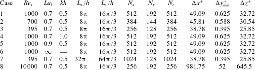
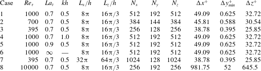
Key parameters of simulation cases.
2.2 Simulation cases
Table 1 summarizes the key parameters of the simulation cases used to study the localizing effect of LCs on background turbulence, including the Reynolds number  $Re_{\unicode[STIX]{x1D70F}}=u_{\unicode[STIX]{x1D70F}}h/\unicode[STIX]{x1D708}$, with
 $\unicode[STIX]{x1D708}$ being the kinematic viscosity, dimensionless wavenumber
 $kh$, turbulent Langmuir number
 $La_{t}$, computational domain size
 $L_{x}\times L_{y}\times L_{z}$, number of grid points
 $N_{x}\times N_{y}\times N_{z}$, and grid resolution
 $\unicode[STIX]{x0394}x^{+}$,
 $\unicode[STIX]{x0394}y_{min}^{+}$ and
 $\unicode[STIX]{x0394}z^{+}$. In this paper, the superscript ‘
 $^{+}$’ is used to denote non-dimensional quantities normalized using wall units
 $\unicode[STIX]{x1D708}/u_{\unicode[STIX]{x1D70F}}$ and the friction velocity
 $u_{\unicode[STIX]{x1D70F}}$ as the characteristic length and velocity scales, respectively. The computational domain size is set to
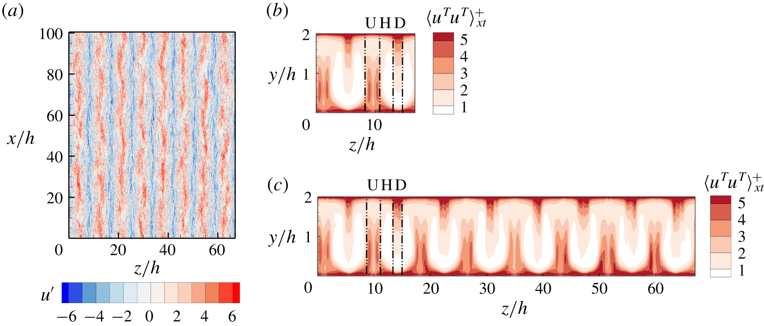
 $8\unicode[STIX]{x03C0}h\times 2h\times 16\unicode[STIX]{x03C0}h/3$ in cases 1–6. To ensure that this computational domain size is sufficiently large to capture the localizing effects of LCs on the background turbulence, we conducted another simulation with a larger computational domain size of
 $32\unicode[STIX]{x03C0}h\times 2h\times 64\unicode[STIX]{x03C0}h/3$, denoted as case 7 in table 1. The other parameters of case 7 are the same as those of case 3. It is shown in the Appendix that the results of cases 3 and 7 are consistent, indicating that the computational domain size for cases 1–6 is sufficient. In the wall-resolved LES cases (cases 1–7), the grid is refined near the bottom and top of the computational domain, and
 $\unicode[STIX]{x0394}y_{min}^{+}$ is the resolution of the first grid near the top or bottom. The grid resolution used in cases 1–7 (table 1) meets the requirement of wall-resolved LES (Chapman Reference Chapman1979; Choi & Moin Reference Choi and Moin2012). In the wall-modelled LES case (case 8), the vertical grid is evenly distributed, and the first point is located in the logarithmic layer (Deng et al. Reference Deng, Yang, Xuan and Shen2019).
In case 1 (table 1), the values of  $kh$ and
 $La_{t}$ are given consistent with the observations in the field (Gargett & Wells Reference Gargett and Wells2007), and as such this case is used to start the analyses of the localizing effects of LCs on the background turbulence. Other cases are then used to examine the localizing effect of LCs at various
 $Re_{\unicode[STIX]{x1D70F}}$,
 $La_{t}$ and
 $kh$ shown in §§ 5 and 6. From case 1 to case 3, the Reynolds number changes from 1000 to 395 to study the influence of the Reynolds number, while the values of
 $La_{t}$ and
 $kh$ remain unchanged. Case 8 is conducted to study the localizing effects of LCs on background turbulence at a practical Reynolds numbers
 $Re_{\unicode[STIX]{x1D70F}}=10^{4}$. To investigate the effect of the wavenumber
 $kh$, its value is set to 0.5 and 1.0 in cases 1 and 4, respectively. The effect of
 $La_{t}$ is studied by comparing the results of cases 1 and 5, in which the values of
 $La_{t}$ are set to 0.7 and 0.9, respectively. Case 6 without the vortex forcing is used as a reference case for the velocity scaling study in § 5.
2.3 Definition of turbulence statistics
To analyse the localizing effect of LCs on the background turbulence, the velocity is decomposed into the mean velocity  $\langle u_{i}\rangle$, the LC content velocity
 $u_{i}^{L}$ and the background turbulence velocity fluctuations
 $u_{i}^{T}$ as
 $$\begin{eqnarray}u_{i}(x,y,z,t)=\langle u_{i}\rangle (y)+{u_{i}}^{\prime }(x,y,z,t)=\langle u_{i}\rangle (y)+u_{i}^{L}(y,z,t)+u_{i}^{T}(x,y,z,t).\end{eqnarray}$$
Because all the quantities studied in this paper are implicitly filtered at the grid level, the overline is omitted to simplify the presentations hereinafter. A pair of angular brackets  $\langle \cdot \rangle$ is used to denote the time and plane averaging, viz.
 $$\begin{eqnarray}\langle u_{i}\rangle (y)=\frac{1}{L_{x}L_{z}(T_{2}-T_{1})}\int _{T_{1}}^{T_{2}}\int _{0}^{L_{z}}\int _{0}^{L_{x}}u_{i}(x,y,z,t)\,\text{d}x\,\text{d}z\,\text{d}t.\end{eqnarray}$$
Here,  $T_{1}$ and
 $T_{2}$ indicate the starting and ending instants of the time interval, respectively. The total velocity fluctuation
 $u_{i}^{\prime }$ is defined as the difference between
 $u_{i}$ and
 $\langle u_{i}\rangle$. Because the LCs are elongated in the streamwise direction, the LC content velocity
 $u_{i}^{L}$ is extracted using the streamwise averaging as
 $$\begin{eqnarray}u_{i}^{L}(y,z,t)=\langle u_{i}^{\prime }\rangle _{x}(y,z,t)=\frac{1}{L_{x}}\int _{0}^{L_{x}}u_{i}^{\prime }(x,y,z,t)\,\text{d}x,\end{eqnarray}$$
where  $\langle \cdot \rangle _{x}$ stands for the averaging in the streamwise direction
 $x$. The background turbulence velocity
 $u_{i}^{T}$ is then defined as
 $$\begin{eqnarray}u_{i}^{T}(x,y,z,t)=u_{i}^{\prime }(x,y,z,t)-u_{i}^{L}(y,z,t).\end{eqnarray}$$
The present triple decomposition given by (2.6) has the same spirit as but different form from the one proposed by Reynolds & Hussain (Reference Reynolds and Hussain1972), in which the velocity field is decomposed into the time-averaged mean flow, the organized wave motion and the turbulent motion based on the characteristic temporal frequency of the components. In contrast, the present triple decomposition is based on the characteristic spatial length scale of different components. The triple decomposition used in the present study is similar to that introduced by Papavassiliou & Hanratty (Reference Papavassiliou and Hanratty1997) in their investigation of Couette cells in turbulent Couette flows and later applied by Tejada-Martínez & Grosch (Reference Tejada-Martínez and Grosch2007) in their analysis of LCs in shallow-water Langmuir turbulence. According to Tejada-Martínez & Grosch (Reference Tejada-Martínez and Grosch2007), the present triple decomposition based on the spatial length scale is effective in capturing the LCs.
From the definition of velocity fluctuations, it is known that
 $$\begin{eqnarray}\langle u_{i}^{\prime }\rangle =\langle u_{i}^{\prime }\rangle _{xzt}=0.\end{eqnarray}$$
Substituting the definition of  $u_{i}^{L}$ given by (2.8) into (2.10), it is found that
 $$\begin{eqnarray}\langle u_{i}^{L}\rangle _{zt}=0.\end{eqnarray}$$
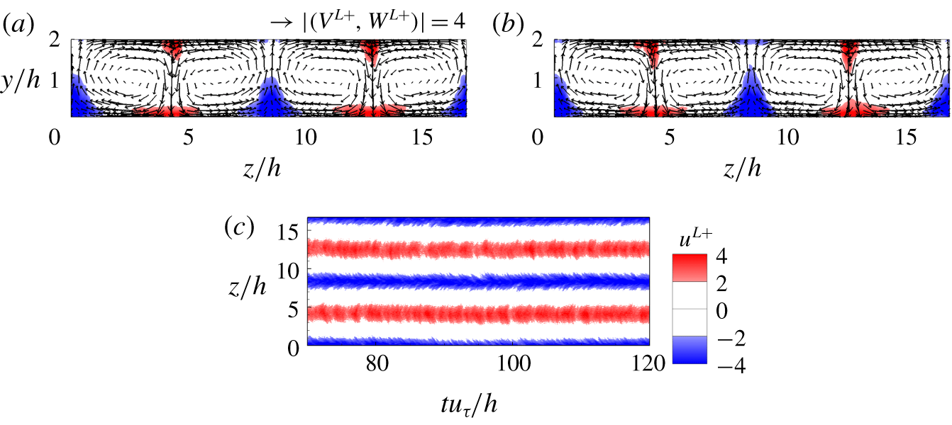
However, because  $u_{i}^{L}$ is inhomogeneous in the spanwise direction (figure 1) but homogeneous in time, the spanwise averaging is not equivalent to time averaging. As a result, the time averaging of
 $u_{i}^{L}$ is not zero, i.e.
 $$\begin{eqnarray}\langle u_{i}^{L}\rangle _{t}\neq 0.\end{eqnarray}$$
A non-zero time-averaged  $u_{i}^{L}$ was also found when the Couette cells (Papavassiliou & Hanratty Reference Papavassiliou and Hanratty1997) or full-depth LCs (Tejada-Martínez & Grosch Reference Tejada-Martínez and Grosch2007) exist.
Spatial and temporal variation of the LC content velocity  $u_{i}^{L}$. (a,b) Instantaneous fields of
 $u_{i}^{L}$ in a cross-stream plane at
 $tu_{\unicode[STIX]{x1D70F}}/h=175$ and
 $295$, respectively. The contours show the streamwise component
 $u^{L+}$, while the vectors consist of
 $(v^{L+},w^{L+})$. (c) Contours of
 $u^{L+}$ in a
 $z$–
 $t$ plane at
 $y/h=0.1$. The results of case 1 are shown.

Figures 1(a) and 1(b) show the instantaneous flow fields of  $u_{i}^{L}$ in a
 $y$–
 $z$ plane at times
 $tu_{\unicode[STIX]{x1D70F}}/h=175$ and
 $295$, respectively. It can be observed that LCs appear in the pattern of counter-rotating vortex pairs, accompanied by positive and negative LC content streamwise velocity (
 $u^{L}$) in the downwelling and upwelling limbs, respectively. The pattern of contours and vectors shown in figure 1(a,b) is consistent with the results of Tejada-Martínez & Grosch (Reference Tejada-Martínez and Grosch2007). By contrasting figure 1(a) with figure 1(b), it is evident that the LC content velocity fields at two different instants are similar, indicating that the spanwise location of the LCs remains almost unchanged during the simulation. This observation can further be confirmed using the time history of the LC content velocity. Figure 1(c) displays the contours of
 $u^{L}$ in a
 $z$–
 $t$ plane at the vertical location
 $y/h=0.1$. It is shown that the contours of
 $u^{L}$ are nearly stationary in time, indicating that the spanwise location of the LCs is approximately fixed. In field measurements in coastal regions, the full-depth LCs are transient mainly due to their spanwise movement induced by the spanwise tidal motion (Gargett & Wells Reference Gargett and Wells2007). However, the characteristic time scale of the background turbulence is much shorter than that of LCs, such that the LCs can be regarded as persistent structures in the analyses of the localization effect of LCs on the background turbulence. It has also been demonstrated that most of the statistics obtained from the LES of Tejada-Martínez & Grosch (Reference Tejada-Martínez and Grosch2007) in the absence of the spanwise tidal motion agree with those obtained from the field measurement of Gargett & Wells (Reference Gargett and Wells2007).
Because the spanwise locations of streamwise-elongated LCs remain stable over time, the LC content velocities significantly vary only with the vertical and spanwise coordinates in the  $y$–
 $z$ plane. The localizing effect of LCs on the background turbulence can be revealed by comparing the distribution of the intensities of background turbulence in the
 $y$–
 $z$ plane with that of the LC content velocity. Therefore, time and streamwise averaging is used to define the localized Reynolds stresses as
 $$\begin{eqnarray}\langle u_{i}^{T}u_{j}^{T}\rangle _{xt}(y,z)=\frac{1}{L_{x}(T_{2}-T_{1})}\int _{T_{1}}^{T_{2}}\int _{0}^{L_{x}}u_{i}^{T}(x,y,z,t)u_{j}^{T}(x,y,z,t)\,\text{d}x\,\text{d}t,\end{eqnarray}$$
where  $\langle \cdot \rangle _{xt}$ denotes the time and streamwise averaging. The time-averaged statistics shown herein are obtained using over 1200 instantaneous snapshots, corresponding to a time duration of
 $T_{2}-T_{1}=120h/u_{\unicode[STIX]{x1D70F}}$. To examine if the number of snapshots is sufficient, we compared the results based on 1200 and 600 snapshots. It was observed that reducing the number of snapshots by half results in a change in
 $\langle u_{i}^{T}v_{j}^{T}\rangle _{xt}$ by less than
 $1.2\,\%$.
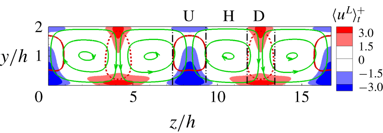
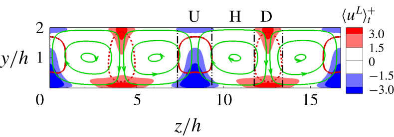
Based on the time-averaged vertical component of the LC content velocity,  $\langle v^{L}\rangle _{t}$, the spanwise location can be divided into the downwelling-motion region (D-region), upwelling-motion region (U-region) and horizontal-motion region (H-region) as shown schematically in figure 2, which displays the contours of
 $\langle u^{L}\rangle _{t}$ and isopleths of
 $\langle v^{L}\rangle _{t}=\pm 0.3\max (\langle v^{L}\rangle _{t})$. Hereinafter,
 $\langle \cdot \rangle _{t}$ represents averaging in time. The streamlines are superimposed to show the location of the LCs. The three regions are separated by dash-dotted lines, defined as the vertical tangent lines of the isopleths of
 $\langle v^{L}\rangle _{t}=\pm 0.3\max (|\langle v^{L}\rangle _{t}|)$. In the D-region and U-region, the vertical motions of LCs are strong, characterized by large negative and positive values of
 $\langle v^{L}\rangle _{t}$, respectively. In the H-region, the spanwise motion of LCs is dominant, while the magnitude of
 $\langle v^{L}\rangle _{t}$ is relatively small.
Time-averaged LC content velocity field  $\langle u_{i}^{L}\rangle _{t}^{+}$. The contours show the value of
 $\langle u^{L}\rangle _{t}^{+}$, the solid and dashed black lines represent the isopleth of
 $\langle v^{L}\rangle _{t}^{+}=0.3\max (\langle v^{L}\rangle _{t})$ and
 $-0.3\max (\langle v^{L}\rangle _{t})$, respectively, and the solid green lines with arrows are the streamlines of LCs on the vertical
 $y$–
 $z$ plane. The dash-dotted black vertical lines divide the spanwise locations into the U-, H- and D-regions, which are dominated by the upwelling, spanwise and downwelling motions of the LCs, respectively. The results of case 1 are shown.
3 Localizing effect of LCs on background turbulence
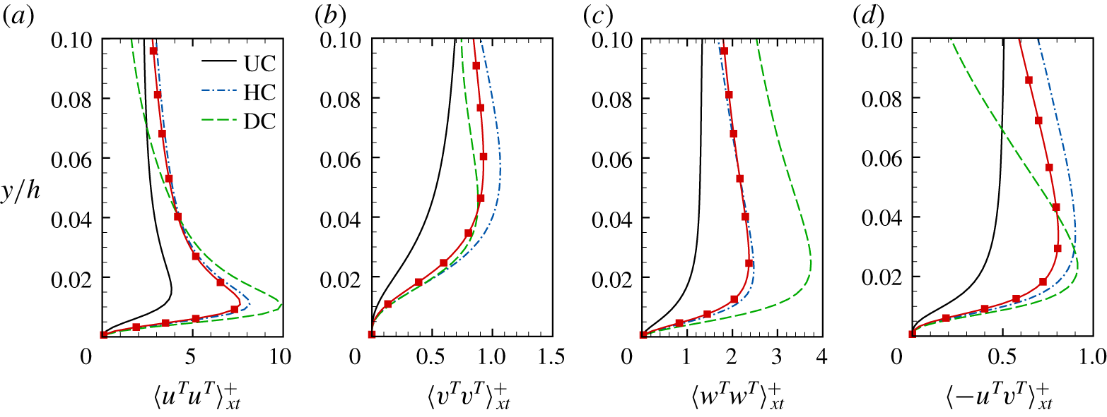
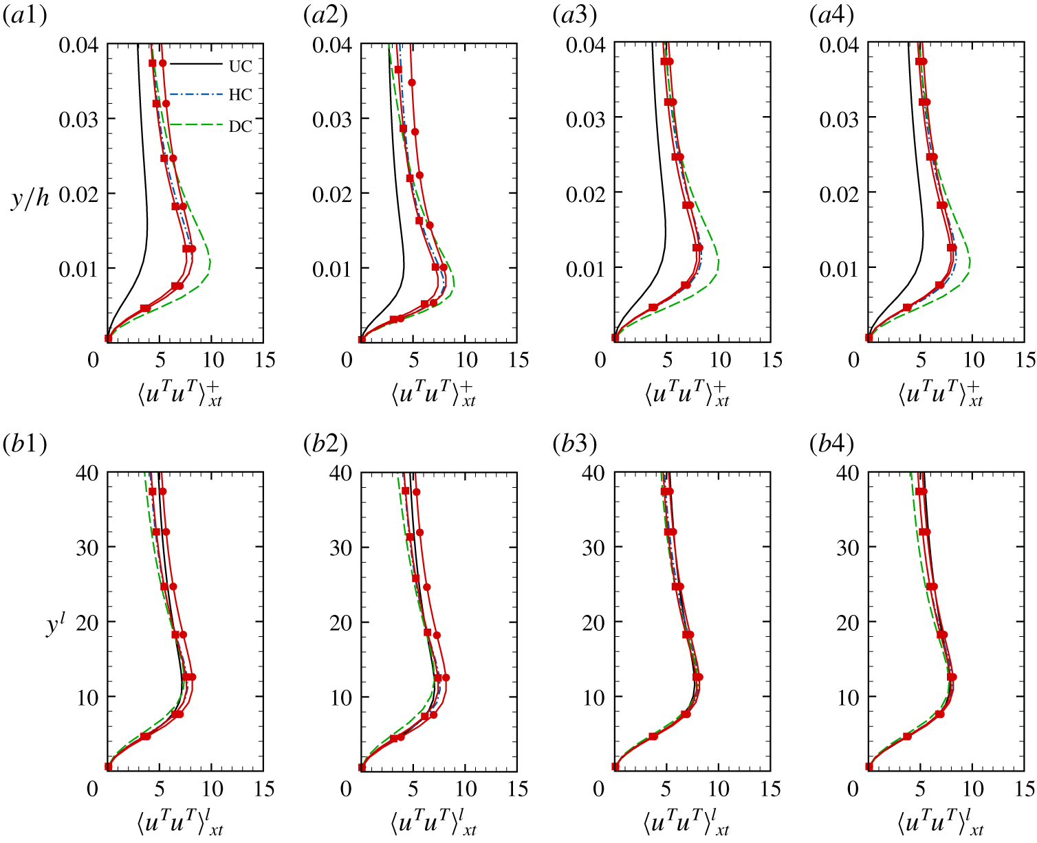
In this section, the localizing effect of LCs on the background turbulence is studied using case 1 as a representative case. Other cases are used to examine the localizing effect at various parameters in § 5. The localizing effects of LCs on the background turbulence can be studied quantitatively using the localized Reynolds stresses  $\langle u_{i}^{T}u_{j}^{T}\rangle _{xt}$. Let DC, HC and UC denote the spanwise centres of the D-region, H-region and U-region, respectively. Figure 3 compares the vertical profiles of
 $\langle u_{i}^{T}u_{j}^{T}\rangle _{xt}$ near the water bottom (
 $y/h\leqslant 0.1$) at DC, HC and UC. Figure 3(a) shows that, below
 $y/h=0.04$, the magnitude of
 $\langle u^{T}u^{T}\rangle _{xt}$ is larger at DC than at HC and UC. It is striking that the peak value of
 $\langle u^{T}u^{T}\rangle _{xt}$ at DC is approximately three times that at UC. Although a localizing effect of large-scale motions on small-scale streamwise velocity was also observed in wall-bounded turbulence without LCs (Mathis et al. Reference Mathis, Hutchins and Marusic2009; Inoue et al. Reference Inoue, Mathis, Marusic and Pullin2012), the localizing effect of LCs on
 $u^{T}$ is much more significant in the shallow-water Langmuir turbulence studied here. For example, in turbulent channel flows, the magnitude ratio between
 $\langle u^{T}u^{T}\rangle _{xt}$ collocating with positive and negative large-scale streamwise velocity is only 1.2 (Jimenez Reference Jimenez2012; Deng et al. Reference Deng, Huang and Xu2016), while this ratio is approximately
 $3.0$ in the shallow-water Langmuir turbulence. As the distance from the bottom increases from
 $y/h=0.015$ to 0.1, the value of
 $\langle u^{T}u^{T}\rangle _{xt}$ decreases faster at DC than at UC and HC. Consequently, the magnitude of
 $\langle u^{T}u^{T}\rangle _{xt}$ at DC becomes smaller than that at HC and UC above
 $y/h=0.04$ and 0.07, respectively. From figure 3(b), it is seen that the magnitude of
 $\langle v^{T}v^{T}\rangle _{xt}$ is smaller at UC than at both HC and DC below
 $y/h=0.1$. Below
 $y/h=0.02$, the magnitudes of
 $\langle v^{T}v^{T}\rangle _{xt}$ at HC and DC are comparable, while above
 $y/h=0.02$, the intensity of
 $v^{T}$ is stronger at HC than at DC. Figure 3(c) shows that the magnitudes of
 $\langle w^{T}w^{T}\rangle _{xt}$ at DC and UC are, respectively, the largest and smallest among the three spanwise locations.
Vertical profiles of localized Reynolds stresses  $\langle u_{i}^{T}u_{j}^{T}\rangle _{xt}$ at UC, HC and DC near the water bottom: (a)
 $\langle u^{T}u^{T}\rangle _{xt}$, (b)
 $\langle v^{T}v^{T}\rangle _{xt}$, (c)
 $\langle w^{T}w^{T}\rangle _{xt}$ and (d)
 $\langle -u^{T}v^{T}\rangle _{xt}$. The lines with squares represent the Reynolds stresses
 $\langle u_{i}^{T}u_{j}^{T}\rangle$ based on the time and plane averaging. The results of case 1 are shown.
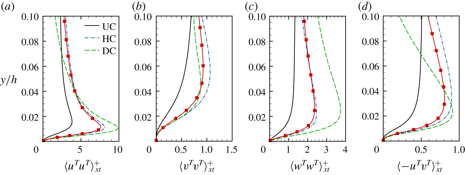
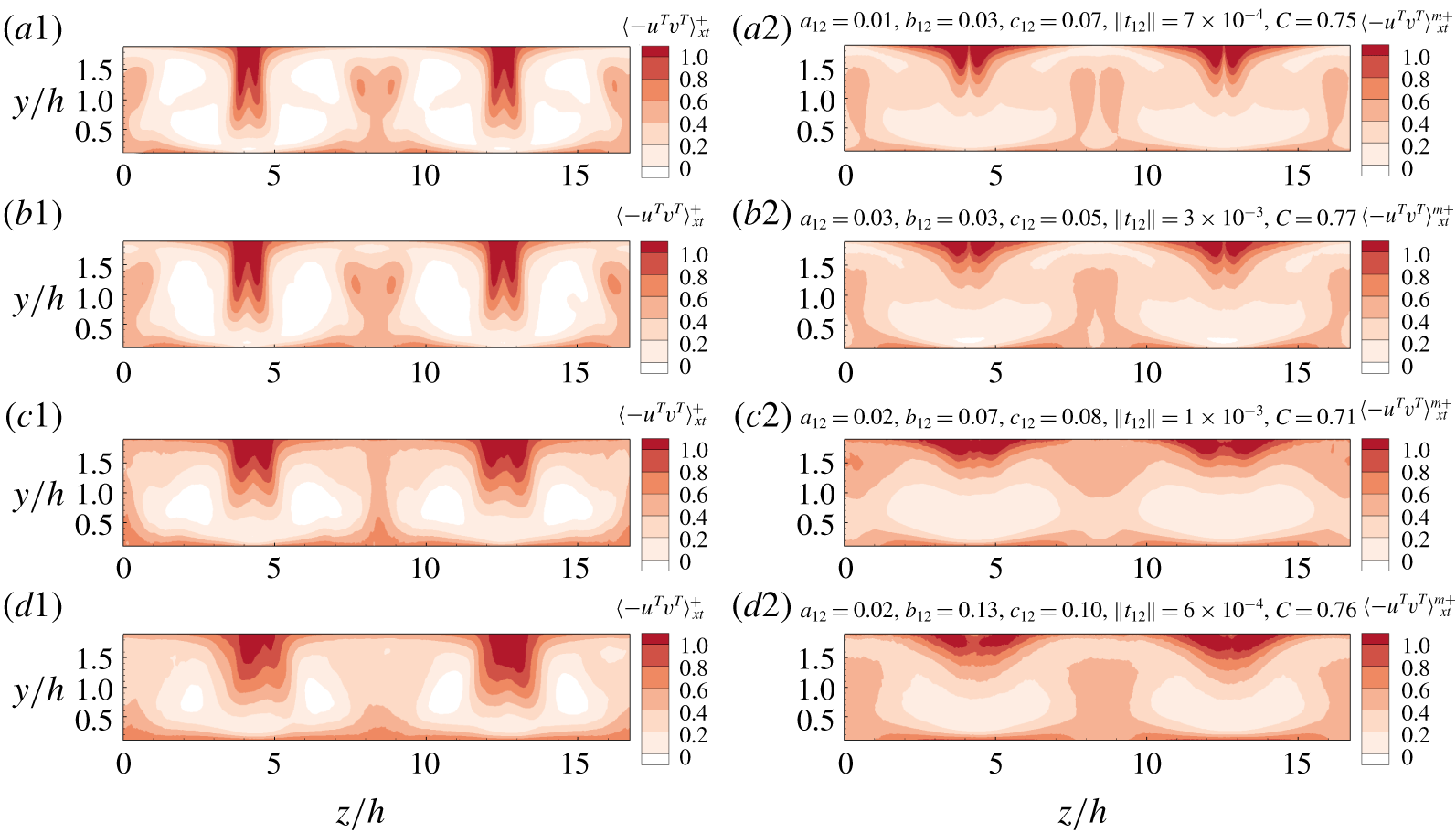
The above results of the localized Reynolds normal stresses reveal the localizing effect of LCs on the intensity of the background turbulence. Correspondingly, the momentum flux of the background turbulence is also localized by the LCs. As shown in figure 3(d), below  $y/h=0.03$, the magnitudes of the localized Reynolds shear stress
 $\langle -u^{T}v^{T}\rangle _{xt}$ at DC and UC are, respectively, larger and smaller than that at HC, indicating the enhancement and suppression of momentum flux in the D- and U-regions, respectively. As the distance from the bottom increases to
 $y/h\geqslant 0.03$ and
 $y/h\geqslant 0.07$, the magnitude of
 $\langle -u^{T}v^{T}\rangle$ at DC becomes smaller than that at HC and UC, respectively. Such a change in the localizing effect of LCs on
 $\langle -u^{T}v^{T}\rangle$ is similar to that on
 $\langle u^{T}u^{T}\rangle$.
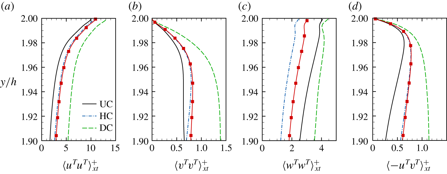
Vertical profiles of localized Reynolds stresses  $\langle u_{i}^{T}u_{j}^{T}\rangle _{xt}$ at UC, HC and DC near the surface: (a)
 $\langle u^{T}u^{T}\rangle _{xt}$, (b)
 $\langle v^{T}v^{T}\rangle _{xt}$, (c)
 $\langle w^{T}w^{T}\rangle _{xt}$ and (d)
 $\langle -u^{T}v^{T}\rangle _{xt}$. The lines with squares represent the Reynolds stresses
 $\langle u_{i}^{T}u_{j}^{T}\rangle$ based on the time and plane averaging. The results of case 1 are shown.
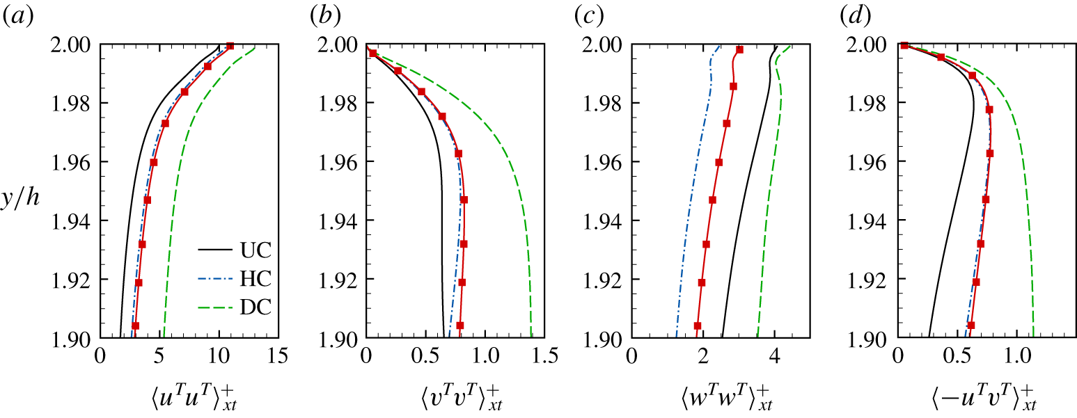
To explore the localizing effect of LCs on the background turbulence in the near-surface region, the vertical profiles of  $\langle u_{i}^{T}u_{j}^{T}\rangle _{xt}$ for
 $y/h\geqslant 1.9$ at DC, HC and UC are compared in figure 4. The localizing effects of LCs on
 $\langle u^{T}u^{T}\rangle _{xt}$,
 $\langle v^{T}v^{T}\rangle _{xt}$ and
 $\langle -u^{T}v^{T}\rangle _{xt}$ are similar near the surface. As shown in figure 4(a,b,d), their magnitudes are, respectively, smaller and larger at UC and DC than at HC. The localizing effect on
 $\langle w^{T}w^{T}\rangle _{xt}$ is different from the other three components in the near-surface region. The magnitude of
 $\langle w^{T}w^{T}\rangle _{xt}$ is larger at UC and DC than at HC (figure 4c). The localizing effects of LCs on the background turbulence shown above statistically can also be observed from the instantaneous fields of
 $u_{i}^{T}$ at
 $y/h=0.015$ and
 $1.985$ in §A of the supplementary material (available at https://doi.org/10.1017/jfm.2020.215).
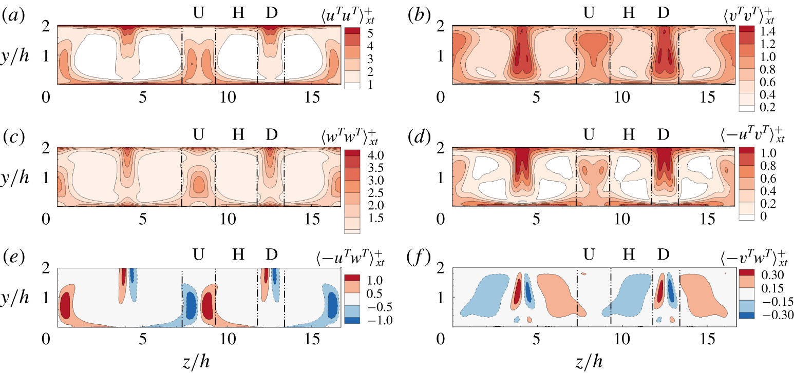
Contours of localized Reynolds stresses  $\langle u_{i}^{T}u_{j}^{T}\rangle _{xt}$ on the vertical
 $y$–
 $z$ plane: (a)
 $\langle u^{T}u^{T}\rangle _{xt}$, (b)
 $\langle v^{T}v^{T}\rangle _{xt}$, (c)
 $\langle w^{T}w^{T}\rangle _{xt}$, (d)
 $\langle -u^{T}v^{T}\rangle _{xt}$, (e)
 $\langle -u^{T}w^{T}\rangle _{xt}$ and (f)
 $\langle -v^{T}w^{T}\rangle _{xt}$. The results of case 1 are shown.
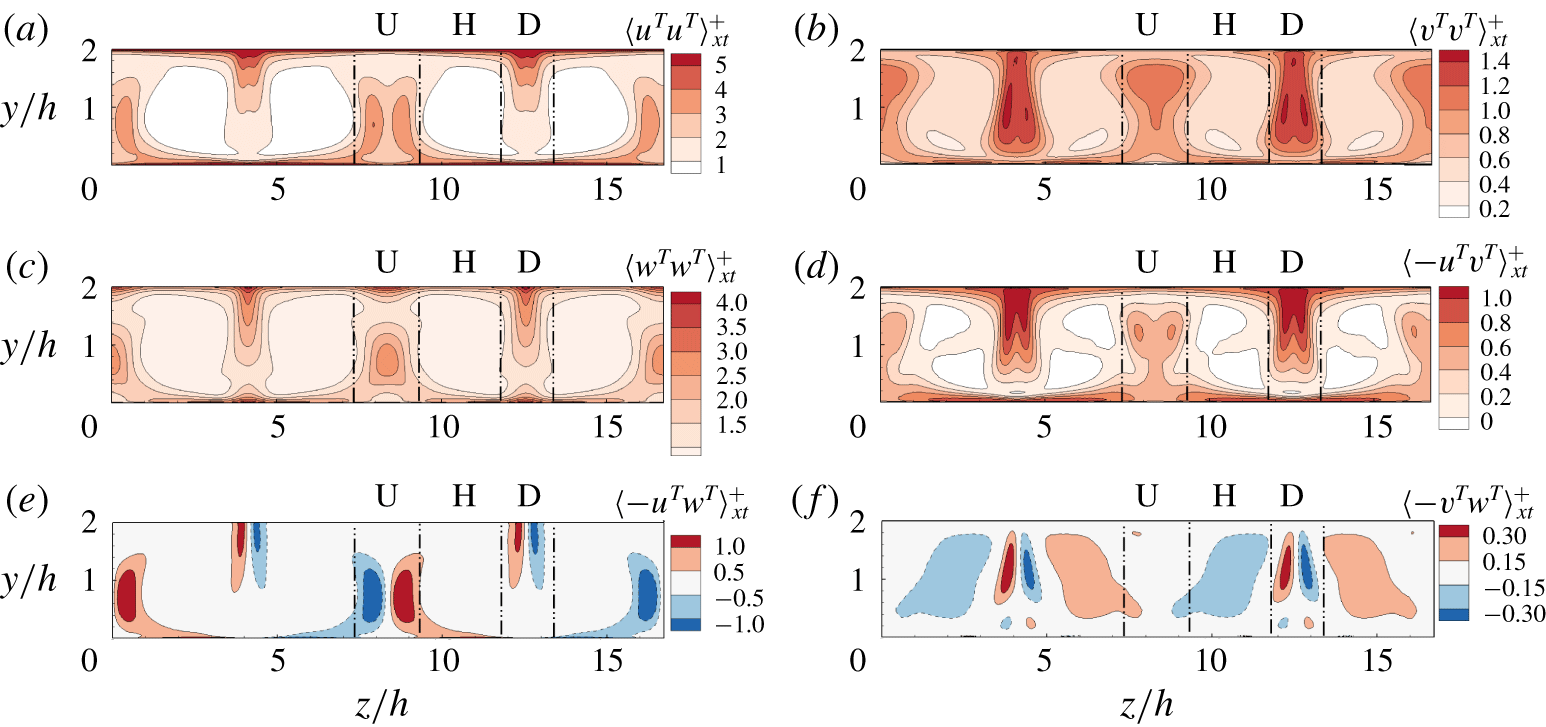
The LCs also influence the background turbulence in the central region of the water column. Figure 5 shows the contours of  $\langle u_{i}^{T}u_{j}^{T}\rangle _{xt}$ in the
 $y$–
 $z$ plane. It is observed from figure 5(a–f) that, except for
 $\langle -v^{T}w^{T}\rangle _{xt}^{+}$, the effects of LCs on the other five components of
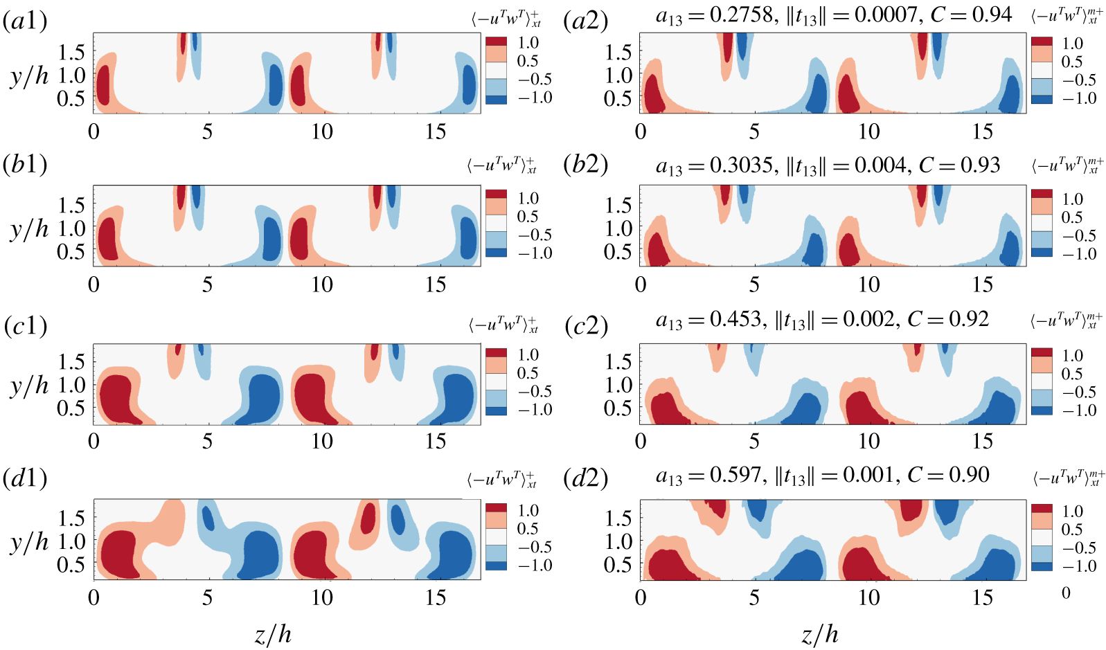
 $\langle u_{i}^{T}u_{j}^{T}\rangle _{xt}^{+}$ are similar in the central region of the water column. There are two regions where the magnitudes of
 $\langle u_{i}^{T}u_{j}^{T}\rangle$ are enhanced. These two regions are located in the U-region and D-region, connecting with the water bottom and water surface, respectively. The strong large-scale vertical motions of LCs in the U- and D-regions promote the vertical transport of scalar and momentum throughout the water column (Kukulka & Harcourt Reference Kukulka and Harcourt2017). Moreover, the locally strong
 $v^{T}$ and
 $\langle -u^{T}v^{T}\rangle _{xt}$ in the U- and D-regions also enhance the vertical transport in the central region of the water column. On the other hand, while the large-scale spanwise motions of LCs are weak in the central region, the strong
 $w^{T}$ and
 $\langle -u^{T}w^{T}\rangle _{xt}$ can induce scalar and momentum transport along the spanwise direction in the D- and U-regions. Compared with other components of
 $\langle u_{i}^{T}u_{j}^{T}\rangle _{xt}^{+}$, the localizing effects of LCs on
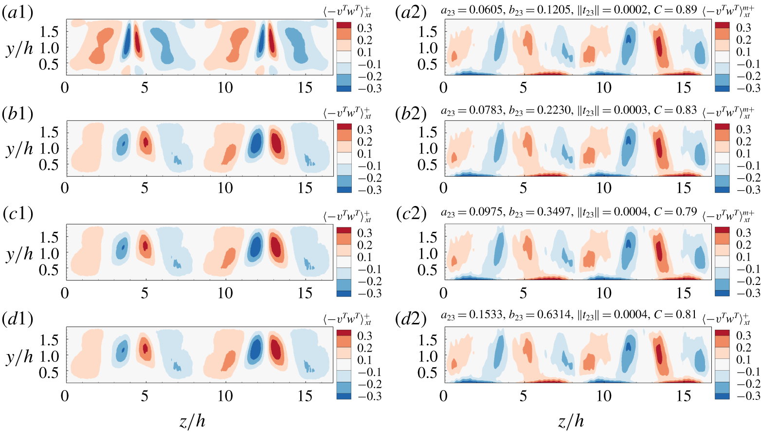
 $\langle -v^{T}w^{T}\rangle$ are different. As shown in figure 5(f),
 $\langle -v^{T}w^{T}\rangle _{xt}^{+}$ is suppressed in the U-region and enhanced in the D-region. Furthermore,
 $\langle -v^{T}w^{T}\rangle _{xt}^{+}$ is smaller in magnitude than other components of
 $\langle u_{i}^{T}u_{j}^{T}\rangle _{xt}$, indicating that
 $\langle -v^{T}w^{T}\rangle _{xt}^{+}$ does not play an important role in the shallow-water Langmuir turbulence. A comparison of the spanwise variation of
 $\langle u_{i}^{T}u_{j}^{T}\rangle _{xt}$ near the bottom, in the central region and near the surface indicates that the localizing effects of LCs are different in these three regions, which is further explained by analysing the transport equations of
 $\langle u_{i}^{T}u_{j}^{T}\rangle _{xt}$ in § 4.
4 Budget of localized Reynolds stresses
4.1 Transport equations of localized Reynolds stresses
In this section, the mechanism underlying the localizing effect of LCs on background turbulence is studied through the analyses of the budget terms in the transport equations of the localized Reynolds stresses, which can be written as
 $$\begin{eqnarray}\displaystyle & & \displaystyle \frac{\unicode[STIX]{x2202}\langle u_{i}^{T}u_{j}^{T}\rangle _{xt}}{\unicode[STIX]{x2202}t}+(\langle u_{k}\rangle +u_{k}^{S})\frac{\unicode[STIX]{x2202}\langle u_{i}^{T}u_{j}^{T}\rangle _{xt}}{\unicode[STIX]{x2202}x_{k}}\nonumber\\ \displaystyle & & \displaystyle \quad =P_{ij}^{M}+\unicode[STIX]{x1D6F1}_{ij}+D_{ij}+T_{ij}+V_{ij}+\unicode[STIX]{x1D700}_{ij}+S_{ij}+P_{ij}^{L}+T_{ij}^{L}.\end{eqnarray}$$
The budget terms on the right-hand side of the above equation are the mean-shear production term  $P_{ij}^{M}$, pressure diffusion term
 $\unicode[STIX]{x1D6F1}_{ij}$, pressure–strain correlation term
 $D_{ij}$, background turbulence diffusion term
 $T_{ij}$, viscous diffusion term
 $V_{ij}$, dissipation term
 $\unicode[STIX]{x1D700}_{ij}$, Stokes forcing term
 $S_{ij}$, LC content production term
 $P_{ij}^{L}$ and LC content turbulence diffusion term
 $T_{ij}^{L}$, respectively. These are defined as follows:
 $$\begin{eqnarray}\displaystyle & \displaystyle P_{ij}^{M}=-\langle u_{j}^{T}u_{k}^{T}\rangle _{xt}\frac{\unicode[STIX]{x2202}\langle u_{i}\rangle }{\unicode[STIX]{x2202}x_{k}}-\langle u_{i}^{T}u_{k}^{T}\rangle _{xt}\frac{\unicode[STIX]{x2202}\langle u_{j}\rangle }{\unicode[STIX]{x2202}x_{k}}, & \displaystyle\end{eqnarray}$$
 $$\begin{eqnarray}\displaystyle & \displaystyle \unicode[STIX]{x1D6F1}_{ij}=-\frac{\unicode[STIX]{x2202}\langle p^{T}u_{j}^{T}\rangle _{xt}}{\unicode[STIX]{x2202}x_{i}}-\frac{\unicode[STIX]{x2202}\langle p^{T}u_{i}^{T}\rangle _{xt}}{\unicode[STIX]{x2202}x_{j}}, & \displaystyle\end{eqnarray}$$
 $$\begin{eqnarray}\displaystyle & \displaystyle D_{ij}=\left\langle p^{T}\left(\frac{\unicode[STIX]{x2202}u_{j}^{T}}{\unicode[STIX]{x2202}x_{i}}+\frac{\unicode[STIX]{x2202}u_{i}^{T}}{\unicode[STIX]{x2202}x_{j}}\right)\right\rangle _{xt}, & \displaystyle\end{eqnarray}$$
 $$\begin{eqnarray}\displaystyle & \displaystyle T_{ij}=-\frac{\unicode[STIX]{x2202}\langle u_{i}^{T}u_{j}^{T}u_{k}^{T}\rangle _{xt}}{\unicode[STIX]{x2202}x_{k}}, & \displaystyle\end{eqnarray}$$
 $$\begin{eqnarray}\displaystyle & \displaystyle V_{ij}=\frac{\unicode[STIX]{x2202}}{\unicode[STIX]{x2202}x_{k}}\left\langle \unicode[STIX]{x1D708}\frac{\unicode[STIX]{x2202}u_{i}^{T}u_{j}^{T}}{\unicode[STIX]{x2202}x_{k}}+u_{j}^{T}(\unicode[STIX]{x1D70F}_{ik}^{sgs})^{T}+u_{i}^{T}(\unicode[STIX]{x1D70F}_{jk}^{sgs})^{T}\right\rangle _{xt}, & \displaystyle\end{eqnarray}$$
 $$\begin{eqnarray}\displaystyle & \displaystyle \unicode[STIX]{x1D700}_{ij}=-\left\langle 2\unicode[STIX]{x1D708}\frac{\unicode[STIX]{x2202}u_{i}^{T}}{\unicode[STIX]{x2202}x_{k}}\frac{\unicode[STIX]{x2202}u_{j}^{T}}{\unicode[STIX]{x2202}x_{k}}+(\unicode[STIX]{x1D70F}_{ik}^{sgs})^{T}\frac{\unicode[STIX]{x2202}u_{j}^{T}}{\unicode[STIX]{x2202}x_{k}}+(\unicode[STIX]{x1D70F}_{jk}^{sgs})^{T}\frac{\unicode[STIX]{x2202}u_{i}^{T}}{\unicode[STIX]{x2202}x_{k}}\right\rangle _{xt}, & \displaystyle\end{eqnarray}$$
 $$\begin{eqnarray}\displaystyle & \displaystyle S_{ij}=-\langle u_{i}^{T}u_{k}^{T}\rangle _{xt}\frac{\unicode[STIX]{x2202}u_{k}^{S}}{\unicode[STIX]{x2202}x_{j}}-\langle u_{j}^{T}u_{k}^{T}\rangle _{xt}\frac{\unicode[STIX]{x2202}u_{k}^{S}}{\unicode[STIX]{x2202}x_{i}}, & \displaystyle\end{eqnarray}$$
 $$\begin{eqnarray}\displaystyle & \displaystyle P_{ij}^{L}=-\left\langle u_{j}^{T}u_{k}^{T}\frac{\unicode[STIX]{x2202}u_{i}^{L}}{\unicode[STIX]{x2202}x_{k}}+u_{i}^{T}u_{k}^{T}\frac{\unicode[STIX]{x2202}u_{j}^{L}}{\unicode[STIX]{x2202}x_{k}}\right\rangle _{xt}, & \displaystyle\end{eqnarray}$$
 $$\begin{eqnarray}\displaystyle & \displaystyle T_{ij}^{L}=-\frac{\unicode[STIX]{x2202}\langle u_{i}^{T}u_{j}^{T}u_{k}^{L}\rangle _{xt}}{\unicode[STIX]{x2202}x_{k}}. & \displaystyle\end{eqnarray}$$
The derivation of the budget equation can be found in § B of the supplementary material. We note here that, because the SGS stress tensor  $\unicode[STIX]{x1D70F}_{ik}^{sgs}$ is a nonlinear function of the velocity, it needs to be treated as a whole to obtain
 $(\unicode[STIX]{x1D70F}_{ik}^{sgs})^{T}$. Specifically,
 $\unicode[STIX]{x1D70F}_{ik}^{sgs}$ is first calculated as a function of
 $x$,
 $y$,
 $z$ and
 $t$ using the dynamic Smagorinsky model (Smargorinsky Reference Smargorinsky1963; Germano et al. Reference Germano, Piomelli, Moin and Cabot1991; Lilly Reference Lilly1992). The triple decomposition given by (2.6)–(2.9) is then applied to obtain
 $(\unicode[STIX]{x1D70F}_{ik}^{sgs})^{T}$. Compared with the transport equations of
 $\langle u_{i}^{\prime }u_{j}^{\prime }\rangle$ (Harcourt Reference Harcourt2013; Sinha et al. Reference Sinha, Tejada-Martínez, Akan and Grosch2015), besides the replacement of the total velocity fluctuation
 $u_{i}^{\prime }$ by the background turbulence velocity fluctuation
 $u_{i}^{T}$ in (4.1)–(4.10), the above transport equations are different from those of
 $\langle u_{i}^{\prime }u_{j}^{\prime }\rangle$ in two respects. First, there are two extra terms,
 $P_{ij}^{L}$ and
 $T_{ij}^{L}$, which indicate the direct impact of the LCs on the localized Reynolds stresses. Secondly, only the time and streamwise averaging is applied in (4.1)–(4.10), so that the spanwise variation of these terms can be obtained to reveal their roles in the localization of
 $\langle u_{i}^{T}u_{j}^{T}\rangle _{xt}$. Similar to § 3, case 1 is used as a representation to study the transport equations of the localized Reynolds stresses. Other cases are used to examine the predictive models for the localized Reynolds stresses proposed in § 5 based on the mechanisms discussed in this section.
4.2 Budget terms of  $\langle u_{i}^{T}u_{j}^{T}\rangle _{xt}$ near the bottom

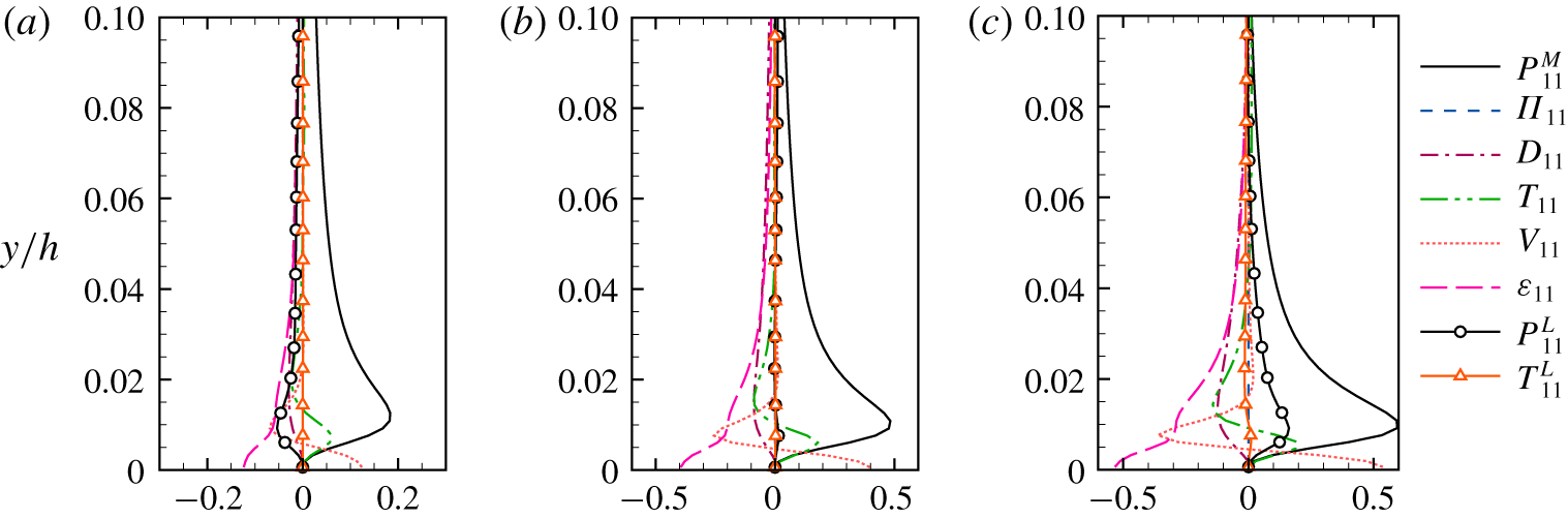
Vertical profiles of budget terms in the transport equation of  $\langle u^{T}u^{T}\rangle _{xt}$ near the bottom at (a) UC, (b) HC and (c) DC. The results of case 1 are shown. The budget terms are scaled by
 $u_{\unicode[STIX]{x1D70F}}^{4}/\unicode[STIX]{x1D708}$.

We start the analyses of the budget balance of  $\langle u_{i}^{T}u_{j}^{T}\rangle _{xt}$ with the near-bottom region first. Figure 6 shows the vertical profiles of the budget terms of
 $\langle u^{T}u^{T}\rangle _{xt}$ in the near-bottom region at UC, HC and DC. The dominant source of
 $\langle u^{T}u^{T}\rangle _{xt}$ is the mean-shear production term
 $P_{11}^{M}$. The expression of
 $P_{11}^{M}$ given by (4.2) can be further simplified to
 $$\begin{eqnarray}P_{11}^{M}=2\langle -u^{T}v^{T}\rangle _{xt}\frac{\text{d}\langle u\rangle }{\text{d}y}.\end{eqnarray}$$
Because the value of  $\text{d}\langle u\rangle /\text{d}y$ is independent of
 $z$, the spanwise variation of
 $P_{11}^{M}$ is completely induced by the localizing effect of the LCs on
 $\langle -u^{T}v^{T}\rangle _{xt}$. From the vertical profiles of
 $\langle -u^{T}v^{T}\rangle _{xt}$ shown in figure 3(d), it is known that, below
 $y/h=0.03$, the magnitude of
 $P_{11}^{M}$ is larger at DC than at HC and UC, while the magnitude of
 $P_{11}^{M}$ at DC becomes smaller than that at HC and UC for
 $y/h\geqslant 0.03$ and
 $y/h\geqslant 0.07$, respectively. Below
 $y/h=0.04$, the LC content production term
 $P_{11}^{L}$ is another important term in the budget balance of
 $\langle u^{T}u^{T}\rangle _{xt}$. From figure 6, it is seen that the value of
 $P_{11}^{L}$ is negative and positive at UC and DC, respectively. Such a spanwise variation of
 $P_{11}^{L}$ tends to suppress and enhance the intensity of
 $u^{T}$ in the U-region and D-region, respectively.
The combined effect of the two production terms  $P_{11}^{M}$ and
 $P_{11}^{L}$ is the dominant reason that leads to the spanwise variation of
 $\langle u^{T}u^{T}\rangle _{xt}$. Below
 $y/h=0.03$, the effects of
 $P_{11}^{M}$ and
 $P_{11}^{L}$ are consistent; both tend to amplify
 $\langle u^{T}u^{T}\rangle _{xt}$ at DC, and, as a result, the magnitude of
 $\langle u^{T}u^{T}\rangle _{xt}$ is larger at DC than at both UC and HC (figure 3a). Between
 $y/h=0.03$ and 0.04, although the magnitude of
 $P_{11}^{M}$ is slightly smaller at DC than at HC, the magnitude of
 $\langle u^{T}u^{T}\rangle _{xt}$ is still larger at DC due to the contribution of the positive LC content production term
 $P_{11}^{L}$. Above
 $y/h=0.04$, the contribution of
 $P_{11}^{L}$ is negligibly small at all of the three spanwise locations, and, consequently, the localizing effect of LCs on
 $\langle u^{T}u^{T}\rangle _{xt}$ is largely correlated with
 $P_{11}^{M}$ or equivalently
 $\langle -u^{T}v^{T}\rangle _{xt}$ (figure 3d). This explains the observation from figure 3(a) that the magnitude of
 $\langle u^{T}u^{T}\rangle _{xt}$ at DC is smaller than that at HC and UC for
 $y/h\geqslant 0.04$ and
 $y/h\geqslant 0.07$, respectively.
Vertical profiles of budget terms in the transport equation of  $\langle v^{T}v^{T}\rangle _{xt}$ near the bottom at (a) UC, (b) HC and (c) DC. The results of case 1 are shown. The budget terms are scaled by
 $u_{\unicode[STIX]{x1D70F}}^{4}/\unicode[STIX]{x1D708}$.
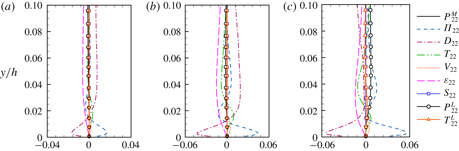
Figure 7 shows the profiles of the budget terms in the transport equation of  $\langle v^{T}v^{T}\rangle _{xt}$ at various spanwise locations in the near-bottom region. Below
 $y/h=0.02$, the budget is dominated by the balance between the negative pressure–strain correlation term
 $D_{22}$ and the positive pressure diffusion term
 $\unicode[STIX]{x1D6F1}_{22}$ at DC, HC and UC. The magnitude of
 $\unicode[STIX]{x1D6F1}_{22}$ is larger at DC than at HC and UC, indicating that, at DC, more energy is diffused towards the near-bottom region. As a result, the magnitude of
 $\langle v^{T}v^{T}\rangle _{xt}$ is larger at DC than that at HC and UC for
 $y/h<0.02$.
Above  $y/h=0.02$, the pressure–strain correlation term
 $D_{22}$ is the main source of
 $\langle v^{T}v^{T}\rangle _{xt}$ at both UC and HC (figure 7a,b). According to the identity
 $D_{11}+D_{22}+D_{33}=0$, the function of the pressure–strain correlation term is to redistribute energy among
 $\langle u^{T}u^{T}\rangle _{xt}$,
 $\langle v^{T}v^{T}\rangle _{xt}$ and
 $\langle w^{T}w^{T}\rangle _{xt}$ without a net production of energy. At both UC and HC,
 $D_{11}$ is negative in the near-bottom region (figure 6a,b), while
 $D_{22}$ is positive for
 $y/h>0.02$ (figure 7a,b). This indicates that in the U-region and H-region, the vertical motion of the background turbulence,
 $v^{T}$, is mainly sustained by the energy redistributed from the streamwise fluctuations
 $u^{T}$. At UC, due to the magnitude suppression of
 $\langle u^{T}u^{T}\rangle _{xt}$, the energy redistributed to
 $\langle v^{T}v^{T}\rangle _{xt}$ is less than that at HC, such that the magnitude of
 $\langle v^{T}v^{T}\rangle _{xt}$ is smaller at UC than at HC (figure 3b).
At DC, the dominant source of  $\langle v^{T}v^{T}\rangle _{xt}$ is different from that at HC and UC for
 $0.02\leqslant y/h\leqslant 0.1$. As shown in figure 7(c), the magnitude of the pressure–strain correlation term
 $D_{22}$ is small, indicating that, although the energy production of
 $\langle u^{T}u^{T}\rangle _{xt}$ is enhanced below
 $y/h=0.04$ at DC (figure 6c), the energy is not gained by
 $\langle v^{T}v^{T}\rangle _{xt}$ through the redistribution effect of the pressure–strain correlation. Instead, the pressure diffusion term
 $\unicode[STIX]{x1D6F1}_{22}$ and the LC content production term
 $P_{22}^{L}$ act as two dominant sources of
 $\langle v^{T}v^{T}\rangle _{xt}$. However, the summation of
 $\unicode[STIX]{x1D6F1}_{22}$ and
 $P_{22}^{L}$ at DC is slightly smaller than the energy source term
 $D_{22}$ at HC. As a result, the magnitude of
 $\langle v^{T}v^{T}\rangle _{xt}$ at DC is smaller than that at HC for
 $0.02\leqslant y/h\leqslant 0.1$ (figure 3b).
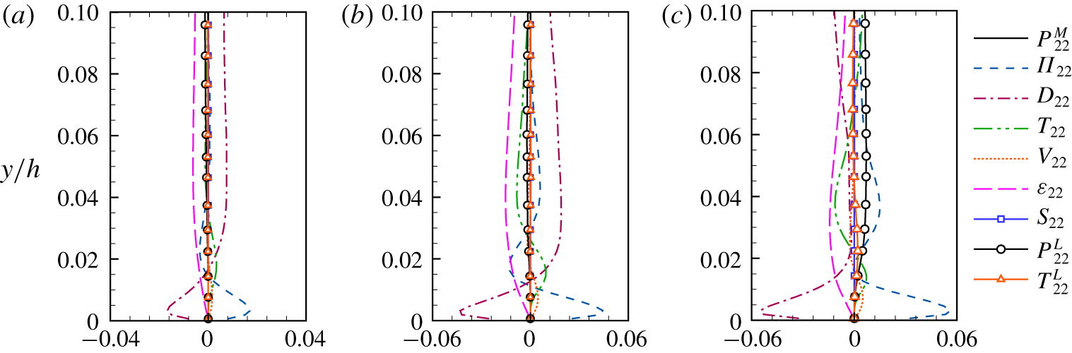
Vertical profiles of budget terms in the transport equation of  $\langle w^{T}w^{T}\rangle _{xt}$ near the bottom at (a) UC, (b) HC and (c) DC. The results of case 1 are shown. The budget terms are scaled by
 $u_{\unicode[STIX]{x1D70F}}^{4}/\unicode[STIX]{x1D708}$.

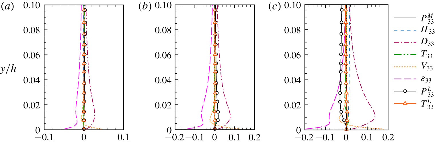
Figure 8 compares the budget balance of  $\langle w^{T}w^{T}\rangle _{xt}$ at UC, HC and DC below
 $y/h=0.1$. It is seen that the pressure–strain correlation term
 $D_{33}$ acts as the dominant source at all of the three spanwise locations. The positively valued
 $D_{33}$ combined with the negatively valued
 $D_{11}$ (figure 6) below
 $y/h=0.1$ redistributes energy from
 $u^{T}$ to
 $w^{T}$. The magnitude of
 $D_{33}$ is smaller at UC than at HC, and is larger at DC than at HC. Correspondingly, the intensity of
 $w^{T}$ is suppressed and enhanced in the U-region and D-region, respectively (figure 3c).
Vertical profiles of budget terms in the transport equation of  $\langle -u^{T}v^{T}\rangle _{xt}$ near the bottom at (a) UC, (b) HC and (c) DC. The results of case 1 are shown. The budget terms are scaled by
 $u_{\unicode[STIX]{x1D70F}}^{4}/\unicode[STIX]{x1D708}$.

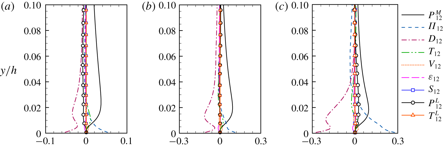
Figure 9 shows the vertical profiles of the budget terms of the localized Reynolds shear stress  $\langle -u^{T}v^{T}\rangle _{xt}$ at UC, HC and DC below
 $y/h=0.1$. The mean-shear production term
 $P_{12}^{M}$ acts as an important source at all of the three spanwise locations. The definition of
 $P_{12}^{M}$ can be rewritten as
 $$\begin{eqnarray}P_{12}^{M}=\langle v^{T}v^{T}\rangle _{xt}\frac{\text{d}\langle u\rangle }{\text{d}y},\end{eqnarray}$$
which indicates that the magnitude of  $P_{12}^{M}$ is proportional to the localized Reynolds normal stress
 $\langle v^{T}v^{T}\rangle _{xt}$. Because
 $\langle v^{T}v^{T}\rangle _{xt}$ (figure 3b) and consequently
 $P_{12}^{M}$ (figure 9a) are reduced at UC,
 $\langle -u^{T}v^{T}\rangle _{xt}$ is suppressed there. Also, from (4.12), it is understood that the magnitude of
 $P_{12}^{M}$ is larger at HC than at DC following
 $\langle v^{T}v^{T}\rangle _{xt}$ (figure 3b). Above
 $y/h=0.03$,
 $P_{12}^{M}$ is the dominant source at both HC and DC, such that the magnitude of
 $\langle -u^{T}v^{T}\rangle _{xt}$ is larger at HC than at DC (figure 9b,c). Below
 $y/h=0.03$, the pressure diffusion term
 $\unicode[STIX]{x1D6F1}_{12}$ acts as another important source, the magnitude of which is larger at DC than at HC. The spanwise variation of
 $\unicode[STIX]{x1D6F1}_{12}$ leads to a larger magnitude of
 $\langle -u^{T}v^{T}\rangle _{xt}$ at DC in comparison with that at HC for
 $y/h\leqslant 0.3$.
4.3 Budget balance of $\langle u_{i}^{T}u_{j}^{T}\rangle _{xt}$ near the surface

Vertical profiles of budget terms in the transport equation of  $\langle u^{T}u^{T}\rangle _{xt}$ near the surface at (a) UC, (b) HC and (c) DC. The results of case 1 are shown. The budget terms are scaled by
 $u_{\unicode[STIX]{x1D70F}}^{4}/\unicode[STIX]{x1D708}$.

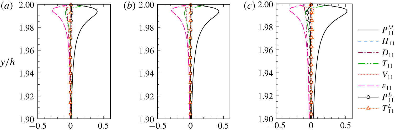
Next, we study the budget balance of the localized Reynolds stresses near the surface. Figure 10 compares the vertical profiles of the budget terms in the transport equation of  $\langle u^{T}u^{T}\rangle _{xt}$ at different spanwise locations UC, HC and DC in the near-surface region for
 $y/h\geqslant 1.9$. The mean-shear production term
 $P_{11}^{M}$ is the dominant source at all of the three spanwise locations. As indicated by (4.11), the magnitude of
 $P_{11}^{M}$ is proportional to that of
 $\langle -u^{T}v^{T}\rangle _{xt}$. Therefore, from the comparison of
 $\langle -u^{T}v^{T}\rangle _{xt}$ at different spanwise locations shown in figure 4(d), it is understood that the magnitude of
 $P_{11}^{M}$ is larger at DC than at HC, and smaller at UC than at HC. This is consistent with the localizing effect of LCs on the magnitude of
 $\langle u^{T}u^{T}\rangle _{xt}$ shown in figure 4(a).
Vertical profiles of budget terms in the transport equation of  $\langle v^{T}v^{T}\rangle _{xt}$ near the surface at (a) UC, (b) HC and (c) DC. The results of case 1 are shown. The budget terms are scaled by
 $u_{\unicode[STIX]{x1D70F}}^{4}/\unicode[STIX]{x1D708}$.

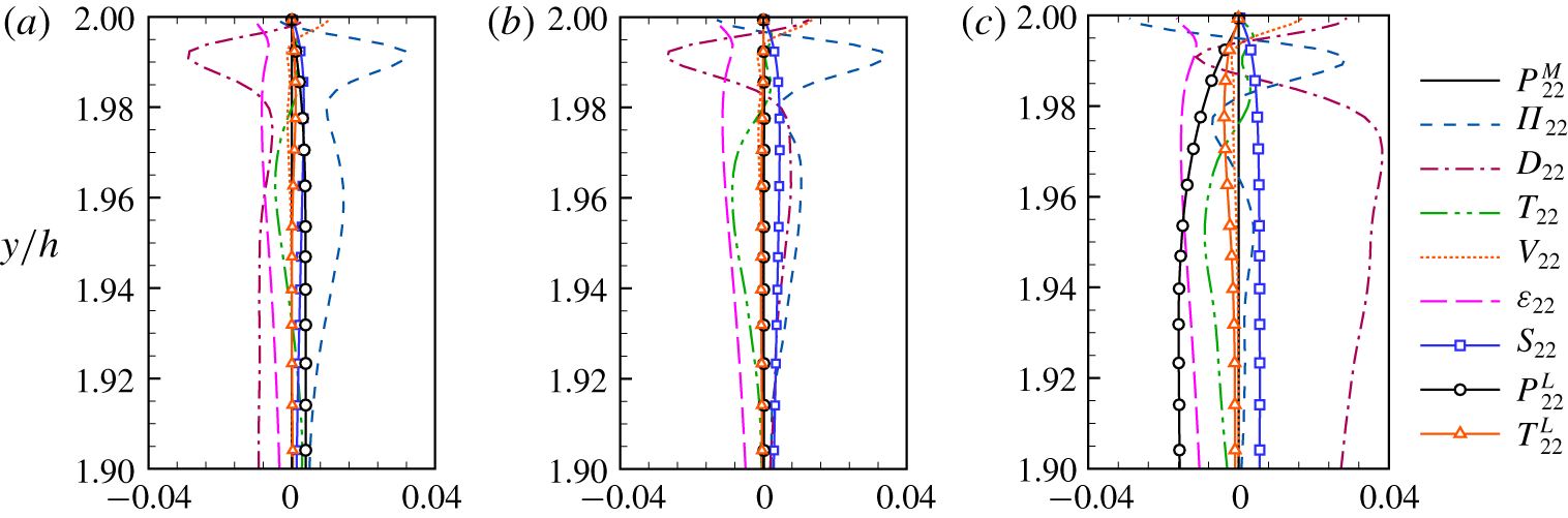
Figure 11 compares the budget balance of  $\langle v^{T}v^{T}\rangle _{xt}$ at UC, HC and DC in the near-surface region. The difference in the role of the pressure–strain correlation term
 $D_{22}$ at UC, HC and DC is one of the most important mechanisms that lead to the localization of
 $\langle v^{T}v^{T}\rangle _{xt}$ near the surface. At UC (figure 11a), the value of
 $D_{22}$ is negative, indicating the loss of energy of
 $v^{T}$ through the energy redistribution. At HC (figure 11b),
 $D_{22}$ is also negative for
 $y/h\geqslant 1.983$, but, as the distance from the surface increases to
 $y/h>1.983$, the role of
 $D_{22}$ changes to a source term of
 $\langle v^{T}v^{T}\rangle _{xt}$. At DC (figure 11c),
 $D_{22}$ acts as the dominant source of
 $\langle v^{T}v^{T}\rangle _{xt}$ for
 $y/h<1.985$, which together with the negative
 $D_{11}$ (figure 10c) redistributes energy from
 $\langle u^{T}u^{T}\rangle _{xt}$ to
 $\langle v^{T}v^{T}\rangle _{xt}$. The magnitude of
 $D_{22}$ at DC is significantly larger than all of the source terms at HC and UC. As a result, the magnitude of
 $\langle v^{T}v^{T}\rangle _{xt}$ is much larger at DC than at both HC and UC (figure 4b).
The primary source for  $\langle v^{T}v^{T}\rangle _{xt}$ at UC and HC (figure 11a,b) is the pressure diffusion term
 $\unicode[STIX]{x1D6F1}_{22}$, indicating an energy flux from the central region of the water column to the near-surface region. The magnitude of
 $\unicode[STIX]{x1D6F1}_{22}$ is comparable between UC and HC in the near-surface region of
 $y/h\geqslant 1.983$, while it is slightly larger at UC than at HC for
 $y/h<1.983$. However, the magnitude of
 $\langle v^{T}v^{T}\rangle$ is slightly smaller at UC than at HC (figure 4b) due to the effects of the Stokes forcing term
 $S_{22}$, the LC content production term
 $P_{22}^{L}$ and the pressure–strain correlation term
 $D_{22}$, as discussed below. Figure 11(a) shows that, in addition to
 $\unicode[STIX]{x1D6F1}_{22}$, both
 $S_{22}$ and
 $P_{22}^{L}$ also act as sources at UC, while
 $S_{22}$ and
 $D_{22}$ feed energy to
 $\langle v^{T}v^{T}\rangle$ at HC (figure 11b). The general expression of the Stokes forcing term
 $S_{22}$ given by (4.8) can be simplified to
 $$\begin{eqnarray}S_{22}=2\langle -u^{T}v^{T}\rangle _{xt}\frac{\text{d}u^{S}}{\text{d}y}.\end{eqnarray}$$
Because  $u^{S}$ is homogeneous in the spanwise direction as defined in (2.4), the spanwise variation of
 $S_{22}$ is induced by
 $\langle -u^{T}v^{T}\rangle _{xt}$, the magnitude of which is smaller at UC than at HC (figure 4d). In this regard, the difference in
 $S_{22}$ between UC and HC is responsible for the phenomenon that the magnitude of
 $\langle v^{T}v^{T}\rangle _{xt}$ is slightly smaller at UC than at HC. Furthermore, the magnitude of
 $P_{22}^{L}$ at UC is smaller than that of
 $D_{22}^{L}$ at HC. This also tends to result in a smaller magnitude of
 $\langle v^{T}v^{T}\rangle$ at UC than at HC.
Vertical profiles of budget terms in the transport equation of  $\langle w^{T}w^{T}\rangle _{xt}$ near the surface at (a) UC, (b) HC and (c) DC. The results of case 1 are shown. The budget terms are scaled by
 $u_{\unicode[STIX]{x1D70F}}^{4}/\unicode[STIX]{x1D708}$.

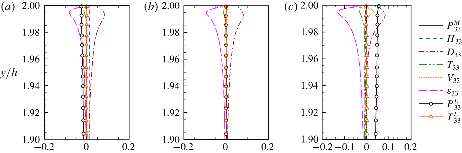
Figure 12 depicts the vertical profiles of the budget terms in the transport equation of  $\langle w^{T}w^{T}\rangle _{xt}$ near the surface. It is seen that the pressure–strain correlation term
 $D_{33}$ is an important source at all of the three spanwise locations. The magnitudes of
 $D_{33}$ at UC, HC and DC are all comparable. At DC, the LC content production term
 $P_{33}^{L}$ acts as an additional source term (figure 12c), which tends to enhance the intensity of
 $w^{T}$. As a result, the magnitude of
 $\langle w^{T}w^{T}\rangle _{xt}$ is larger at DC than at HC and UC (figure 4c). The reason for the difference in the magnitude of
 $\langle w^{T}w^{T}\rangle _{xt}$ between HC and UC (figure 4c) is complex. By contrasting the pressure–strain correlation term
 $D_{33}$ and
 $\unicode[STIX]{x1D6F1}_{33}$ between HC and UC (see § C of the supplementary material), we found that
 $D_{33}$ is comparable at UC and HC. Meanwhile,
 $\unicode[STIX]{x1D6F1}_{33}$ acts as a secondary source at UC, while at HC the contribution of
 $\unicode[STIX]{x1D6F1}_{33}$ in the budget balance is unimportant. The combined effects of
 $D_{33}$ and
 $\unicode[STIX]{x1D6F1}_{33}$ lead to the larger magnitude of
 $\langle w^{T}w^{T}\rangle _{xt}$ at UC than at HC.
Vertical profiles of budget terms in the transport equation of  $\langle -u^{T}v^{T}\rangle _{xt}$ near the surface at (a) UC, (b) HC and (c) DC. The results of case 1 are shown. The budget terms are scaled by
 $u_{\unicode[STIX]{x1D70F}}^{4}/\unicode[STIX]{x1D708}$.

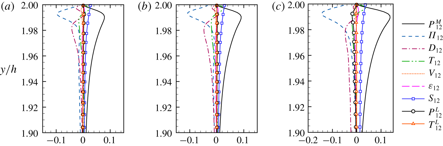
From the above analyses, it is understood that the localized Reynolds shear stress  $\langle -u^{T}v^{T}\rangle _{xt}$ influences the localizing effects on both
 $\langle u^{T}u^{T}\rangle _{xt}$ and
 $\langle v^{T}v^{T}\rangle _{xt}$ near the surface. To further study the reason that leads to the localization of
 $\langle -u^{T}v^{T}\rangle _{xt}$, the vertical profiles of the budget terms of its transport equation in the near-surface region is shown in figure 13. From the figure, it is seen that the mean-shear production term
 $P_{12}^{M}$ and Stokes forcing term
 $S_{12}$ are the primary and secondary source terms, respectively. The expression for
 $S_{12}$ can be simplified from the general one in (4.8) to
 $$\begin{eqnarray}S_{12}=\langle u^{T}u^{T}\rangle _{xt}\frac{\text{d}u^{S}}{\text{d}y}.\end{eqnarray}$$
From (4.12) and (4.14), it is straightforward to see that, because both  $\text{d}\langle u\rangle /\text{d}y$ and
 $\text{d}u^{S}/\text{d}y$ are independent of
 $z$, the spanwise variations of
 $P_{12}^{M}$ and
 $S_{12}$ are induced by
 $\langle v^{T}v^{T}\rangle _{xt}$ and
 $\langle u^{T}u^{T}\rangle _{xt}$, respectively. From the spanwise variations of
 $\langle u^{T}u^{T}\rangle _{xt}$ and
 $\langle v^{T}v^{T}\rangle _{xt}$ near the surface (figure 4a,b), it is evident that the summation of
 $P_{12}^{M}$ and
 $S_{12}$ is larger at DC and smaller at UC than at HC. The localization of the source terms
 $P_{12}^{M}$ and
 $S_{12}$ is consistent with the spanwise variation of
 $\langle -u^{T}v^{T}\rangle _{xt}$ observed in figure 4(d).
4.4 Budgets of $\langle u_{i}^{T}u_{j}^{T}\rangle _{xt}$ in the central region of the water column

In this section, we continue to study the transport equations of the localized Reynolds stresses in the central region of the water column. The objective is to find the dominant process responsible for the localization of the background turbulence. For this purpose, the important source terms are investigated to explain the reason for the large-magnitude  $\langle u_{i}^{T}u_{j}^{T}\rangle _{xt}$ occurring in the U-region and D-region (figure 5).
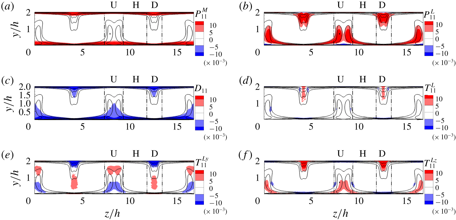
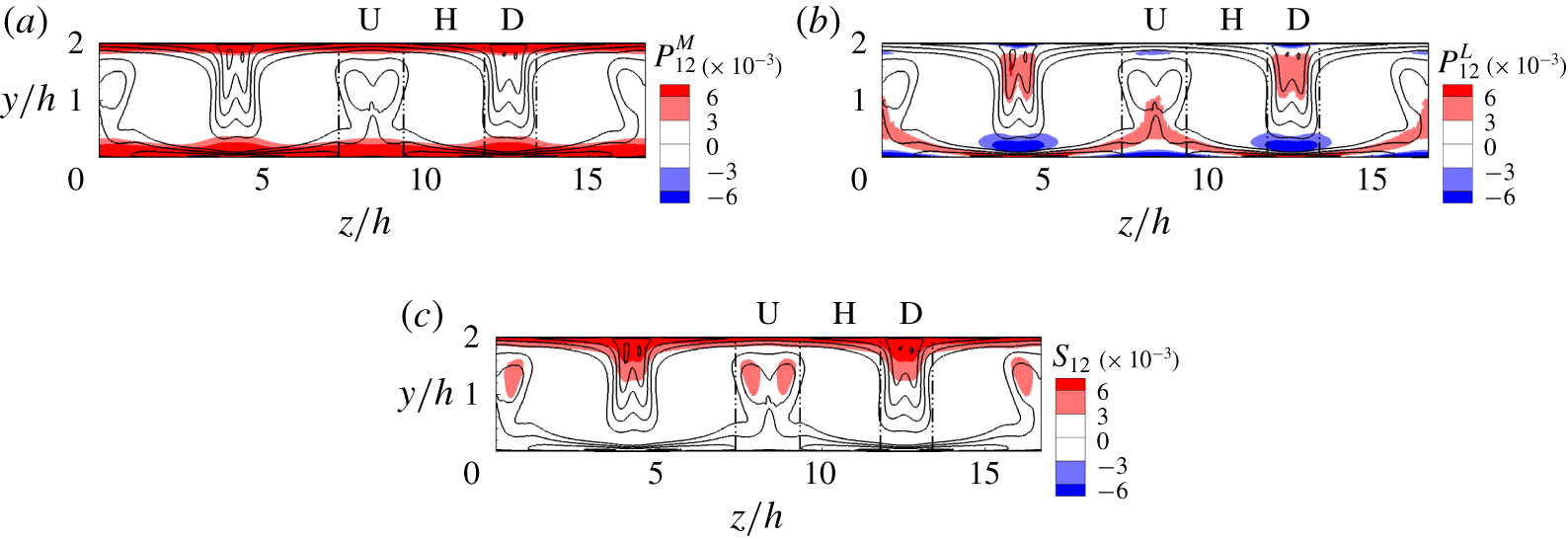
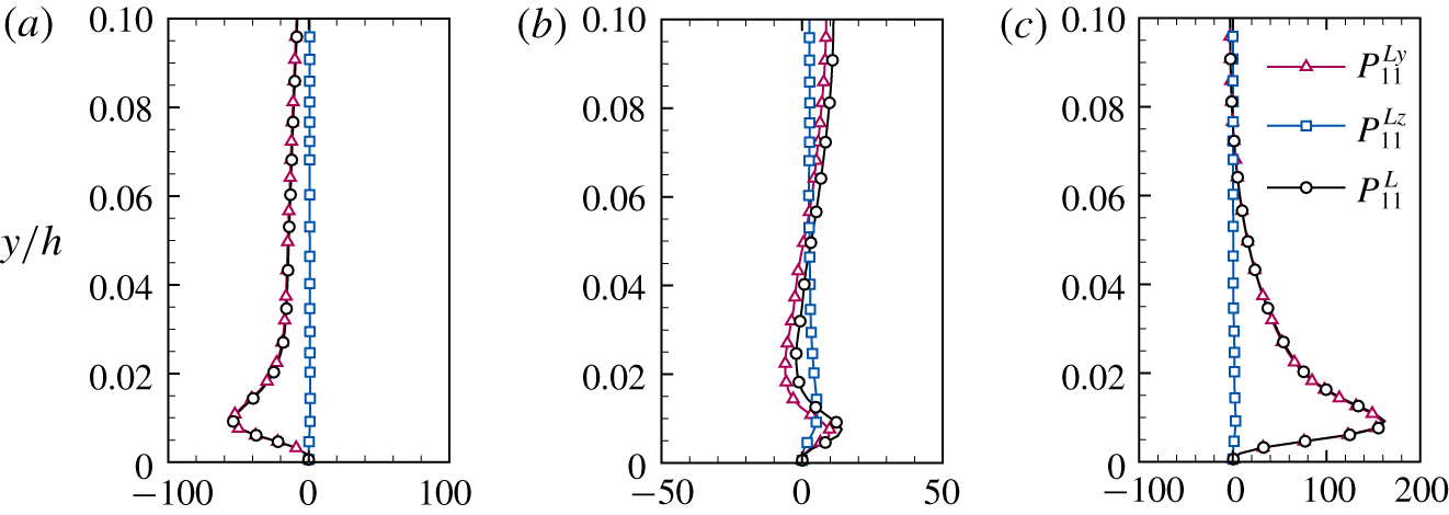
Contours of (a) the mean-shear production term  $P_{11}^{M}$, (b) the LC content production term
 $P_{11}^{L}$, (c) the pressure–strain correlation term
 $D_{11}$ and (d) the LC content turbulent diffusion term
 $T_{11}^{L}$ and its two components (e)
 $T_{11}^{Ly}$ and (f)
 $T_{11}^{Lz}$ in the transport equation of
 $\langle u^{T}u^{T}\rangle _{xt}$ on the vertical
 $y$–
 $z$ plane. These terms are scaled by
 $u_{\unicode[STIX]{x1D70F}}^{4}/\unicode[STIX]{x1D708}$. The isopleths of
 $\langle u^{T}u^{T}\rangle _{xt}^{+}\in [2,5]$ with an interval of 1 are superimposed. The results of case 1 are shown.

Figure 14(a,b) shows the major source terms in the transport equation of  $\langle u^{T}u^{T}\rangle _{xt}$, i.e. the mean-shear production term
 $P_{11}^{M}$ and LC content production term
 $P_{11}^{L}$. The pressure–strain correlation term
 $D_{11}$ is also plotted in figure 14(c), because the energy drained by
 $D_{11}$ is an important source of
 $\langle v^{T}v^{T}\rangle _{xt}$. The LC content turbulent diffusion term
 $T_{11}^{L}$ and its two components
 $T_{11}^{Ly}=-\unicode[STIX]{x2202}\langle u^{T}u^{T}v^{L}\rangle _{xt}/\unicode[STIX]{x2202}y$ and
 $T_{11}^{Lz}=-\unicode[STIX]{x2202}\langle u^{T}u^{T}w^{L}\rangle _{xt}/\unicode[STIX]{x2202}z$ are displayed in figure 14(d–f) to show the effects of the diffusion by the LCs. The terms
 $T_{11}^{Ly}$ and
 $T_{11}^{Lz}$ represent the diffusion induced by the vertical and spanwise motions of LCs, respectively. The isopleths of
 $\langle u^{T}u^{T}\rangle _{xt}$ are superimposed for comparison. Although
 $P_{11}^{M}$ is the dominant source term near the bottom and surface (figures 6 and 10), its magnitude is relatively small in the central region of the water column (figure 14a). Instead,
 $P_{11}^{L}$ acts as the dominant source of
 $\langle u^{T}u^{T}\rangle _{xt}$ in the lower half of the U-region and in the upper half of the D-region (figure 14b). Figure 14(b) also shows that the contour shape of
 $P_{11}^{L}$ is similar to that of
 $\langle u^{T}u^{T}\rangle _{xt}$. From the comparison among the contour patterns of
 $\langle u^{T}u^{T}\rangle _{xt}$,
 $P_{11}^{M}$ and
 $P_{11}^{L}$, it is evident that
 $P_{11}^{L}$ is responsible for the localization of
 $\langle u^{T}u^{T}\rangle _{xt}$ in the central region of the water column.
Compared with the LC content production term  $P_{11}^{L}$, the LC content turbulent diffusion term
 $T_{11}^{L}$ makes a less significant contribution to the localization of
 $\langle u^{T}u^{T}\rangle _{xt}$. As shown, the energy provided by the spanwise convergent motions of LCs in the upper half of the D-region (see
 $T_{11}^{Lz}$ in figure 14f) is mostly diffused to the lower half of the D-region by the downwelling motions of the LCs (see
 $T_{11}^{Ly}$ in figure 14e). As a result, the net contribution of
 $T_{11}^{L}$ to the budget balance of
 $\langle u^{T}u^{T}\rangle _{xt}$ is insignificant in the upper half of the D-region, where
 $\langle u^{T}u^{T}\rangle _{xt}$ is enhanced due to the localizing effect of LCs. Similarly, the balance between
 $T_{11}^{Ly}$ and
 $T_{11}^{Lz}$ in the lower part of the U-region leads to a small net contribution of
 $T_{11}^{L}$ to the large magnitude of
 $\langle u^{T}u^{T}\rangle _{xt}$ there. In the transport equations of other components of
 $\langle u_{i}^{T}u_{j}^{T}\rangle _{xt}$,
 $T_{ij}^{L}$ is not the key process that leads to the localization of
 $\langle u_{i}^{T}u_{j}^{T}\rangle _{xt}$. As a result, they are not further analysed in the following discussions.
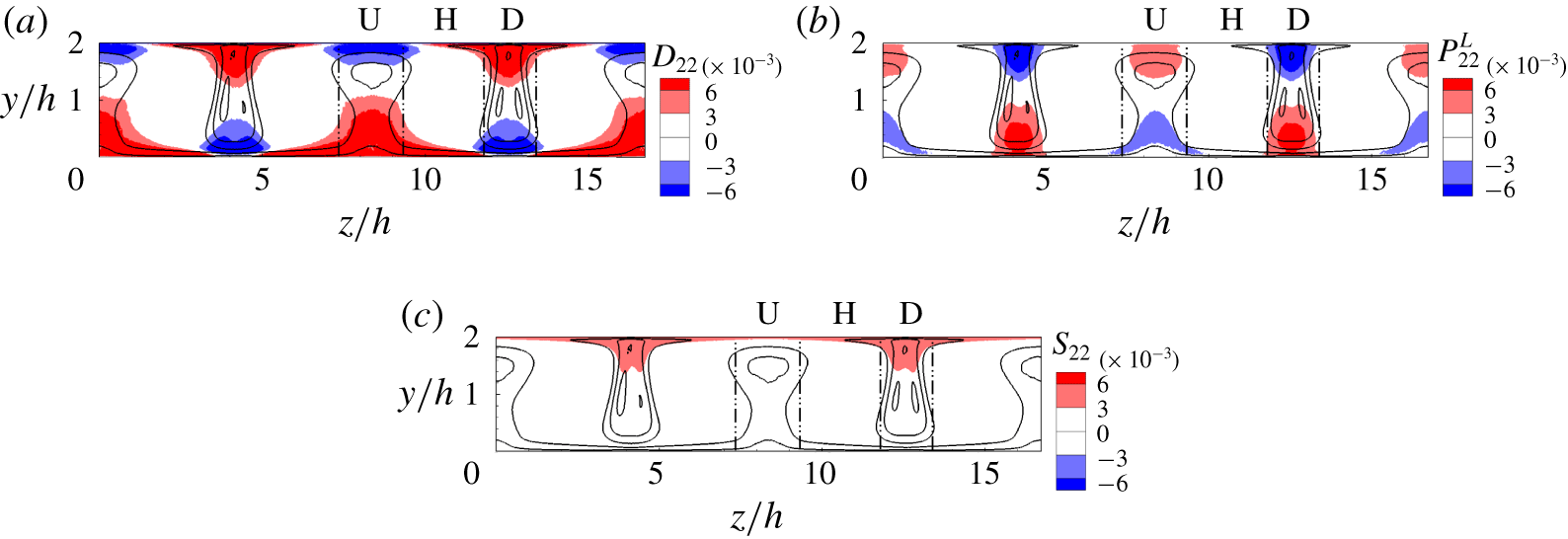
Contours of (a) the pressure–strain correlation term  $D_{22}$, (b) the LC content production term
 $P_{22}^{L}$ and (c) the Stokes forcing term
 $S_{22}$ in the transport equation of
 $\langle v^{T}v^{T}\rangle _{xt}$ on the vertical
 $y$–
 $z$ plane. These terms are normalized by
 $u_{\unicode[STIX]{x1D70F}}^{4}/\unicode[STIX]{x1D708}$. The isopleths of
 $\langle v^{T}v^{T}\rangle _{xt}^{+}\in [0.8,1.4]$ with an interval of 0.3 are superimposed. The results of case 1 are shown.

Figure 15 shows the important terms leading to the localization of  $\langle v^{T}v^{T}\rangle _{xt}$, including the pressure–strain correlation term
 $D_{22}$, the LC content production term
 $P_{22}^{L}$ and the Stokes forcing term
 $S_{22}$. The isopleths of
 $\langle v^{T}v^{T}\rangle _{xt}$ are also displayed for comparison. The value of
 $D_{22}$ is positive in the lower half of the U-region and the upper half of the D-region (figure 15a). From the identity
 $D_{ii}=0$ and the negative
 $D_{11}$, it is understood that the energy gained by
 $\langle v^{T}v^{T}\rangle _{xt}$ through
 $D_{22}$ originates from
 $\langle u^{T}u^{T}\rangle _{xt}$ (figure 14c). As a result, the large-magnitude region of
 $D_{22}$ and
 $\langle v^{T}v^{T}\rangle _{xt}$ collocates with that of
 $D_{11}$ and
 $\langle u^{T}u^{T}\rangle _{xt}$. The large-magnitude contours of
 $\langle v^{T}v^{T}\rangle _{xt}$ in the U-region and D-region extend to the upper and lower half of the water column (figures 5b and 15), respectively, mainly because of the contribution of the LC content production term
 $P_{22}^{L}$ (figure 15b). According to (4.9),
 $P_{22}^{L}$ is equal to
 $-\langle v^{T}v^{T}\rangle _{xt}\unicode[STIX]{x2202}\langle v^{L}\rangle _{t}/\unicode[STIX]{x2202}y-\langle v^{T}w^{T}\rangle _{xt}\unicode[STIX]{x2202}\langle v^{L}\rangle _{t}/\unicode[STIX]{x2202}z$. The large-magnitude
 $-\langle v^{T}w^{T}\rangle _{xt}$ only occurs in the vertical centre of the D-region (figure 5f), and the magnitude of
 $\unicode[STIX]{x2202}\langle v^{L}\rangle _{t}/\unicode[STIX]{x2202}z$ is small near the spanwise centres of both the D- and U-regions due to the maximum magnitude of
 $v^{L}$ there (figure 2). As a result,
 $-\langle v^{T}w^{T}\rangle _{xt}\unicode[STIX]{x2202}\langle v^{L}\rangle _{t}/\unicode[STIX]{x2202}z$ is unimportant in the budget balance of
 $\langle v^{T}v^{T}\rangle _{xt}$. This means that the localization of
 $P_{22}^{L}$ is mainly caused by
 $-\langle v^{T}v^{T}\rangle _{xt}\unicode[STIX]{x2202}\langle v^{L}\rangle _{t}/\unicode[STIX]{x2202}y$. Besides
 $D_{22}$ and
 $P_{22}^{L}$, the Stokes forcing term
 $S_{22}$ provides additional energy to
 $\langle v^{T}v^{T}\rangle _{xt}$ in the upper half of the D-region to enhance the intensity of
 $v^{T}$ there (figure 15c). Because the vertical gradient of the Stokes drift velocity
 $\text{d}u^{S}/\text{d}y$ decreases as the water depth increases, the significant contribution of
 $S_{22}$ to the localizing effect is confined in the upper half of the water column. According to the definition of
 $S_{22}$ in (4.13), because
 $u^{S}$ is homogeneous in the spanwise direction, the spanwise variation of
 $\langle -u^{T}v^{T}\rangle _{xt}$ is responsible for the localization of
 $S_{22}$ in the upper half of the water column.
Contours of (a) the pressure–strain correlation  $D_{33}$ and (b) the LC content production term
 $P_{33}^{L}$ in the transport equation of
 $\langle w^{T}w^{T}\rangle _{xt}$ on the vertical
 $y$–
 $z$ plane. These terms are scaled by
 $u_{\unicode[STIX]{x1D70F}}^{4}/\unicode[STIX]{x1D708}$. The isopleths
 $\langle w^{T}w^{T}\rangle _{xt}^{+}\in [2,4]$ with an interval of
 $1$ are superimposed. The results of case 1 are shown.

Figure 16 compares the contours of the two dominant source terms in the transport equation of  $\langle w^{T}w^{T}\rangle _{xt}$, i.e. the pressure–strain correlation term
 $D_{33}$ and the LC content production term
 $P_{33}^{L}$. The isopleths of
 $\langle w^{T}w^{T}\rangle _{xt}$ are superimposed for further investigations. The pressure–strain correlation term
 $D_{33}$ only makes a significant contribution to
 $\langle w^{T}w^{T}\rangle _{xt}$ near the water bottom and surface, while it is insignificant in the bulk flow. This indicates that the energy redistribution process is not the dominant mechanism underlying the localization of
 $\langle w^{T}w^{T}\rangle _{xt}$ in the central region of the water column. The positive
 $P_{33}^{L}$ in the lower half of the U-region and the upper half of the D-region locally contributes to the enhancement of
 $\langle w^{T}w^{T}\rangle _{xt}$. This is evident from the observation that the contour shape of
 $P_{33}^{L}$ is similar to that of
 $\langle w^{T}w^{T}\rangle _{xt}$ (figure 16b). According to (4.9),
 $P_{33}^{L}$ is equal to
 $-\langle v^{T}w^{T}\rangle _{xt}\unicode[STIX]{x2202}\langle w^{L}\rangle _{t}/\unicode[STIX]{x2202}y-\langle w^{T}w^{T}\rangle _{xt}\unicode[STIX]{x2202}\langle w^{L}\rangle _{t}/\unicode[STIX]{x2202}z$. Although the large-magnitude
 $-\langle v^{T}w^{T}\rangle _{xt}$ only occurs in the vertical centres of the D-region (figure 5f), the magnitude of
 $\unicode[STIX]{x2202}\langle w^{L}\rangle _{t}/\unicode[STIX]{x2202}y$ is small near the spanwise centres of both D- and U-regions due to the small magnitude of
 $w^{L}$ there (figure 2). As a result,
 $-\langle v^{T}w^{T}\rangle _{xt}\unicode[STIX]{x2202}\langle w^{L}\rangle _{t}/\unicode[STIX]{x2202}y$ is unimportant in the budget balance of
 $\langle w^{T}w^{T}\rangle _{xt}$ in the lower half of the U-region and the upper half of the D-region, though
 $P_{33}^{L}$ is of large magnitude in these two regions. This means that the localization of
 $P_{33}^{L}$ is mainly caused by
 $-\langle w^{T}w^{T}\rangle _{xt}\unicode[STIX]{x2202}\langle w^{L}\rangle _{t}/\unicode[STIX]{x2202}z$. Therefore, the localized distribution of
 $\langle w^{T}w^{T}\rangle _{xt}$ is dominated by the LC content production related to
 $\unicode[STIX]{x2202}w^{L}/\unicode[STIX]{x2202}z$.
Contours of (a) the mean-shear production term  $P_{12}^{M}$, (b) the LC content production term
 $P_{12}^{L}$ and (c) the Stokes forcing term
 $S_{12}$ in the transport equation of
 $\langle -u^{T}v^{T}\rangle _{xt}$ on the vertical
 $y$–
 $z$ plane. These terms are scaled by
 $u_{\unicode[STIX]{x1D70F}}^{4}/\unicode[STIX]{x1D708}$. The isopleths of
 $\langle -u^{T}v^{T}\rangle _{xt}^{+}\in [0.2,1.2]$ with an interval of
 $0.25$ are superimposed. The results of case 1 are shown.

The dominant source terms in the transport equation of  $\langle -u^{T}v^{T}\rangle _{xt}$ are plotted in figure 17, including the mean-shear production term
 $P_{12}^{M}$, the LC content production term
 $P_{12}^{L}$ and the Stokes forcing term
 $S_{12}$. As shown in figure 17(a), the magnitude of
 $P_{12}^{M}$ is large near the bottom and surface; but in the central region of the water column,
 $P_{12}^{M}$ is not the primary source in the budget balance of
 $\langle -u^{T}v^{T}\rangle _{xt}$. In the U-region, the LC content production term
 $P_{12}^{L}$ is the dominant source in the lower half of the water column. The large-magnitude contours of
 $\langle -u^{T}v^{T}\rangle _{xt}$ in the U-region extend to the upper half of the water column (figures 5d and 17) mainly because of the contribution of the Stokes forcing term
 $S_{12}$. As shown in figure 17(c),
 $S_{12}$ acts as the dominant source term between
 $y/h=1.0$ and
 $y/h=1.8$ in the U-region. In the D-region,
 $S_{12}$ is the primary source in the upper half of the water column, while
 $P_{12}^{L}$ works as the secondary source. According to the definition of
 $S_{12}$ in (4.14), the large magnitude of
 $S_{12}$ in the upper half of the D-region is due to the enhanced
 $\langle u^{T}u^{T}\rangle _{xt}$.
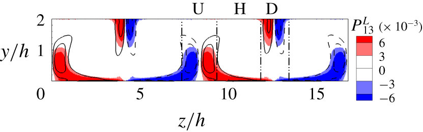
Contours of the LC content production term  $P_{13}^{L}$ in the transport equation of
 $\langle -u^{T}w^{T}\rangle$ on the vertical
 $y$–
 $z$ plane. The term is normalized by
 $u_{\unicode[STIX]{x1D70F}}^{4}/\unicode[STIX]{x1D708}$. The isopleths of
 $\langle -u^{T}w^{T}\rangle _{xt}^{+}=-1.0$,
 $-0.5$,
 $0.5$ and
 $1.0$ are superimposed. The solid and dashed lines represent positive and negative values of
 $\langle -u^{T}w^{T}\rangle _{xt}$, respectively. The results of case 1 are shown.

The dominant source term in the transport equation of  $\langle -u^{T}w^{T}\rangle _{xt}$ is the LC content production term
 $P_{13}^{L}$. The contours of
 $P_{13}^{L}$ and
 $\langle -u^{T}w^{T}\rangle _{xt}$ are displayed in figure 18. It is seen that the sign of
 $P_{13}^{L}$ is consistent with that of
 $\langle -u^{T}w^{T}\rangle _{xt}$, and the regions with large magnitudes of
 $P_{13}^{L}$ and
 $\langle -u^{T}w^{T}\rangle _{xt}$ collocate with each other. The results shown in figure 18 indicate that the LC content production is the dominant factor leading to the localization of
 $\langle -u^{T}w^{T}\rangle _{xt}$.
Contours of (a) the LC content production term  $P_{23}^{L}$ and (b) the Stokes forcing term
 $S_{23}$ in the transport equation of
 $\langle -v^{T}w^{T}\rangle$ on the vertical
 $y$–
 $z$ plane. The term is normalized by
 $u_{\unicode[STIX]{x1D70F}}^{4}/\unicode[STIX]{x1D708}$. The isopleths of
 $\langle -v^{T}w^{T}\rangle _{xt}^{+}=-0.3$,
 $-0.15$,
 $0.15$ and
 $0.3$ are superimposed. The solid and dashed lines represent positive and negative values of
 $\langle -v^{T}w^{T}\rangle _{xt}$, respectively. The results of case 1 are shown.

The dominant source terms in the transport equation of  $\langle -v^{T}w^{T}\rangle _{xt}$ include the LC content production term
 $P_{23}^{L}$ and the Stokes forcing term
 $S_{23}$. The contours of
 $P_{23}^{L}$ and
 $S_{23}$ are compared with those of
 $\langle -u^{T}w^{T}\rangle _{xt}$ in figure 19. As shown, the contours of the large-magnitude
 $\langle -u^{T}w^{T}\rangle _{xt}$ around the vertical centre of the D-region agree with those of
 $P_{23}^{L}$, while
 $S_{23}$ only provides energy near the surface of the D-region. Therefore, the localization of
 $\langle -v^{T}w^{T}\rangle _{xt}$ is attributed to the LC content production.
In summary of the above analyses of the dominant sources in the transport equations of  $\langle u_{i}^{T}u_{j}^{T}\rangle _{xt}$ in the central region of the water column, the key process responsible for the localization of
 $\langle u_{i}^{T}u_{j}^{T}\rangle _{xt}$ is the energy production induced by the LCs. The large magnitude of the positive LC content production in the lower half of the U-region and the upper half of the D-region (figures 14b and 16b) indicates a strong energy cascade from the large-scale LCs to small-scale background turbulence in these two regions. Kukulka et al. (Reference Kukulka, Plueddemann and Sullivan2012) and Martinat et al. (Reference Martinat, Grosch and Gatski2014) also studied the LC content energy production in shallow-water Langmuir turbulence. They used time and plane averaging to define statistics without considering the localizing effects. The LC content production term for
 $\langle u_{i}^{T}u_{j}^{T}\rangle$ (i.e. background turbulence Reynolds stresses based on time and plane averaging) obtained from their simulations is much smaller than that for
 $\langle u_{i}^{T}u_{j}^{T}\rangle _{xt}$ (i.e. localized Reynolds stresses without applying the spanwise averaging) obtained from the present study. The comparison between the LC content production terms in the budget balances of
 $\langle u_{i}^{T}u_{j}^{T}\rangle$ and
 $\langle u_{i}^{T}u_{j}^{T}\rangle _{xt}$ indicates that the spanwise-averaged energy cascade is much weaker than its localized counterpart. This is attributed to the fact that the LC content production for
 $\langle u_{i}^{T}u_{j}^{T}\rangle$ is mainly induced by the vertical gradient of the LC content velocity,
 $\unicode[STIX]{x2202}u_{i}^{L}/\unicode[STIX]{x2202}y$, while the spanwise gradient of the LC content velocity,
 $\unicode[STIX]{x2202}u_{i}^{L}/\unicode[STIX]{x2202}z$, also makes an important contribution to the energy production of the localized Reynolds stress
 $\langle u_{i}^{T}u_{j}^{T}\rangle$. As analysed above, the LC content production of
 $\langle w^{T}w^{T}\rangle$ in the central region of the water column is mainly induced by
 $\unicode[STIX]{x2202}w^{L}/\unicode[STIX]{x2202}z$. As further analysed in § 5,
 $\unicode[STIX]{x2202}u^{L}/\unicode[STIX]{x2202}z$ is essential for the LC content production of
 $\langle u^{T}u^{T}\rangle$ and
 $\langle -u^{T}w^{T}\rangle$.
5 Predictive models of localized Reynolds stresses
Based on the mechanisms underlying the localizing effects of LCs on the background turbulence discussed above, next we propose predictive models for scaling the localized Reynolds stresses and assessing the spatial dependence of Boussinesq-model parameters for localized Reynolds stresses. These models are examined in shallow-water Langmuir turbulence using the LES data with various values of the Reynolds number  $Re_{\unicode[STIX]{x1D70F}}$, the wavenumber
 $kh$ and the turbulent Langmuir number
 $La_{t}$.
5.1 Near the bottom
It is revealed in § 4.2 that the localizing effects of LCs on the magnitude of  $\langle u^{T}u^{T}\rangle _{xt}$ near the bottom are attributed to the spanwise variation in the mean-shear production term
 $P_{11}^{M}$ and LC content production term
 $P_{11}^{L}$. To develop the scaling of
 $\langle u^{T}u^{T}\rangle _{xt}$, the LC content production term
 $P_{ij}^{L}$ in (4.9) is decomposed into two parts,
 $P_{ij}^{Ly}$ and
 $P_{ij}^{Lz}$, defined as
 $$\begin{eqnarray}P_{ij}^{Ly}=-\left\langle u_{j}^{T}u_{k}^{T}\frac{\unicode[STIX]{x2202}u_{i}^{L}}{\unicode[STIX]{x2202}x_{k}}\right\rangle _{xt}\unicode[STIX]{x1D6FF}_{2k}-\left\langle u_{i}^{T}u_{k}^{T}\frac{\unicode[STIX]{x2202}u_{j}^{L}}{\unicode[STIX]{x2202}x_{k}}\right\rangle _{xt}\unicode[STIX]{x1D6FF}_{2k}\end{eqnarray}$$
and
 $$\begin{eqnarray}P_{ij}^{Lz}=-\left\langle u_{j}^{T}u_{k}^{T}\frac{\unicode[STIX]{x2202}u_{i}^{L}}{\unicode[STIX]{x2202}x_{k}}\right\rangle _{xt}\unicode[STIX]{x1D6FF}_{3k}-\left\langle u_{i}^{T}u_{k}^{T}\frac{\unicode[STIX]{x2202}u_{j}^{L}}{\unicode[STIX]{x2202}x_{k}}\right\rangle _{xt}\unicode[STIX]{x1D6FF}_{3k},\end{eqnarray}$$
respectively, with  $\unicode[STIX]{x1D6FF}_{ik}$ being the Kronecker delta symbol. Because
 $u_{i}^{L}$ is defined using streamwise averaging and it changes little with the time (figure 1c),
 $u_{i}^{L}=\langle u_{i}^{L}\rangle _{t}=\langle u_{i}^{L}\rangle _{xt}$ holds approximately. As a result,
 $P_{ij}^{Ly}$ and
 $P_{ij}^{Lz}$ can be further simplified to
 $$\begin{eqnarray}P_{ij}^{Ly}=-\langle u_{j}^{T}u_{k}^{T}\rangle _{xt}\frac{\unicode[STIX]{x2202}\langle u_{i}^{L}\rangle _{t}}{\unicode[STIX]{x2202}x_{k}}\unicode[STIX]{x1D6FF}_{2k}-\langle u_{i}^{T}u_{k}^{T}\rangle _{xt}\frac{\unicode[STIX]{x2202}\langle u_{j}^{L}\rangle _{t}}{\unicode[STIX]{x2202}x_{k}}\unicode[STIX]{x1D6FF}_{2k}\end{eqnarray}$$
and
 $$\begin{eqnarray}P_{ij}^{Lz}=-\langle u_{j}^{T}u_{k}^{T}\rangle _{xt}\frac{\unicode[STIX]{x2202}\langle u_{i}^{L}\rangle _{t}}{\unicode[STIX]{x2202}x_{k}}\unicode[STIX]{x1D6FF}_{3k}-\langle u_{i}^{T}u_{k}^{T}\rangle _{xt}\frac{\unicode[STIX]{x2202}\langle u_{j}^{L}\rangle _{t}}{\unicode[STIX]{x2202}x_{k}}\unicode[STIX]{x1D6FF}_{3k},\end{eqnarray}$$
respectively.
Figure 20 compares the profiles of  $P_{11}^{L}$,
 $P_{11}^{Ly}$ and
 $P_{11}^{Lz}$ at UC, HC and DC. As shown, at all of the three spanwise locations, the profiles of
 $P_{11}^{L}$ and
 $P_{11}^{Ly}$ almost collapse, while the magnitude of
 $P_{11}^{Lz}$ is negligibly small, indicating that, near the bottom, the LC content production is dominated by the interaction between
 $\unicode[STIX]{x2202}\langle u^{L}\rangle _{t}/\unicode[STIX]{x2202}y$ and
 $\langle -u^{T}v^{T}\rangle _{xt}$. The negative
 $P_{11}^{Ly}$ near the bottom of UC implies the localized energy inverse cascade from the small-scale background turbulence to large-scale LCs. Despite the negative
 $P_{11}^{Ly}$ at UC, as shown in the work of Kukulka et al. (Reference Kukulka, Plueddemann and Sullivan2012) and Martinat et al. (Reference Martinat, Grosch and Gatski2014), the time- and plane-averaged
 $P_{11}^{Ly}$ is still positive, indicating the net energy cascade from large-scale LCs to small-scale background turbulence near the bottom.
Vertical profiles of  $P_{11}^{Ly}$,
 $P_{11}^{Lz}$ and
 $P_{11}^{L}$ in the near-bottom region at (a) UC, (b) HC and (c) DC. Here,
 $P_{11}^{Ly}$,
 $P_{11}^{Lz}$ and
 $P_{11}^{L}$ are scaled by
 $u_{\unicode[STIX]{x1D70F}}^{4}/\unicode[STIX]{x1D708}$. The results of case 1 are shown.

Combining (4.11) and (5.3), a total localized production term of  $\langle u^{T}u^{T}\rangle _{xt}$ can be written as
 $$\begin{eqnarray}P_{11}=P_{11}^{M}+P_{11}^{Ly}=2\langle -u^{T}v^{T}\rangle _{xt}\frac{\unicode[STIX]{x2202}\langle u\rangle _{xt}}{\unicode[STIX]{x2202}y},\end{eqnarray}$$
where  $\langle u\rangle _{xt}=\langle u\rangle +u^{L}$ is the localized mean streamwise velocity defined in the same way as the localized Reynolds stress in (2.13). Near the bottom of the D-region, the LC content mean velocity
 $u^{L}$ is positive (figure 2), such that the localized mean velocity
 $\langle u\rangle _{xt}$ and its vertical gradient
 $\unicode[STIX]{x2202}\langle u\rangle _{xt}/\unicode[STIX]{x2202}y$ are larger than the time- and plane-averaged counterparts
 $\langle u\rangle$ and
 $\text{d}\langle u\rangle /\text{d}y$, respectively. In contrast, near the bottom of the U-region, the magnitudes of
 $\langle u\rangle _{xt}$ and
 $\unicode[STIX]{x2202}\langle u\rangle _{xt}/\unicode[STIX]{x2202}y$ are smaller than those of
 $\langle u\rangle$ and
 $\text{d}\langle u\rangle /\text{d}y$, respectively.
Profiles of (a1–4) $\langle u^{T}u^{T}\rangle _{xt}^{+}$ in the coordinate
 $y/h$ and (b1–4)
 $\langle u^{T}u^{T}\rangle _{xt}^{l}$ in the localized near-bottom coordinate
 $y^{l}$: (a1,b1)
 $Re_{\unicode[STIX]{x1D70F}}=1000$,
 $kh=0.5$ and
 $La_{t}=0.7$; (a2,b2)
 $Re_{\unicode[STIX]{x1D70F}}=700$,
 $kh=0.5$ and
 $La_{t}=0.7$; (a3,b3)
 $Re_{\unicode[STIX]{x1D70F}}=1000$,
 $kh=1.0$ and
 $La_{t}=0.7$; and (a4,b4)
 $Re_{\unicode[STIX]{x1D70F}}=1000$,
 $kh=0.5$ and
 $La_{t}=0.9$. The red lines with square symbols are the time- and plane-averaged Reynolds stress
 $\langle u^{T}u^{T}\rangle$ in each case, and the red lines with circle symbols are
 $\langle u^{T}u^{T}\rangle$ in the shear-driven turbulent flow.

The difference in the localized mean velocity gradient indicates that the localized friction Reynolds number also varies in the spanwise direction. In canonical wall turbulence without LCs, it has been found that the profiles of near-bottom  $\langle u^{T}u^{T}\rangle$ scaled by the friction velocity in the vertical coordinate normalized by wall units are insensitive to the friction Reynolds number (Smith, McKeon & Marusic Reference Smith, McKeon and Marusic2011). In view of this, a localized friction velocity is defined as
 $$\begin{eqnarray}u_{l}=\sqrt{\unicode[STIX]{x1D708}\left(\frac{\unicode[STIX]{x2202}\langle u\rangle _{xt}}{\unicode[STIX]{x2202}y}\right)_{y=0}}.\end{eqnarray}$$
Correspondingly, a localized viscous length scale is defined as
 $$\begin{eqnarray}\unicode[STIX]{x1D6FF}_{l}=\unicode[STIX]{x1D708}/u_{l}.\end{eqnarray}$$
The variables normalized using  $u_{l}$ and
 $\unicode[STIX]{x1D6FF}_{l}$ are denoted by the superscript ‘
 $^{l}$’. Figure 21 compares the profiles of
 $\langle u^{T}u^{T}\rangle _{xt}^{+}$ in the coordinate
 $y/h$ and
 $\langle u^{T}u^{T}\rangle _{xt}^{l}$ in the localized near-bottom coordinate
 $y^{l}$. The results of cases 1–4 are displayed to examine the effectiveness of the proposed scaling under various flow conditions. The profiles of time- and plane-averaged Reynolds stress
 $\langle u^{T}u^{T}\rangle ^{+}$ for the corresponding case and shear-driven turbulent flow (case 5) are superimposed for comparison. As shown in figure 21(a1–4), the localizing effects of the LCs on the magnitude of
 $\langle u^{T}u^{T}\rangle ^{+}$ in all cases are consistent. Specifically, the magnitude of
 $\langle u^{T}u^{T}\rangle ^{+}$ is larger at DC than at HC and is smaller at UC than at HC. In contrast, figure 21(b1–4) shows that the profiles of
 $\langle u^{T}u^{T}\rangle ^{l}$ at different spanwise locations collapse in the localized near-bottom coordinate
 $y^{l}$. They are also close to the profile of
 $\langle u^{T}u^{T}\rangle ^{+}$ in the global near-bottom coordinate
 $yu_{\unicode[STIX]{x1D70F}}/\unicode[STIX]{x1D708}$ in the shear-driven turbulence. This indicates that, in the near-bottom region, the profiles of
 $\langle u^{T}u^{T}\rangle _{xt}^{+}$ in Langmuir turbulence under various flow conditions can be predicted using the results in the shear-driven turbulence with proper scalings.
To date, no scaling has been found for the profiles of  $\langle v^{T}v^{T}\rangle$ and
 $\langle w^{T}w^{T}\rangle$ near the bottom at various Reynolds numbers in canonical wall-bounded turbulent flows (Smith et al. Reference Smith, McKeon and Marusic2011; Bernardini, Pirozzoli & Orlandi Reference Bernardini, Pirozzoli and Orlandi2014; Deng et al. Reference Deng, Huang and Xu2016). The main reason is that the dominant energy sources of
 $\langle v^{T}v^{T}\rangle$ and
 $\langle w^{T}w^{T}\rangle$ are the pressure–strain correlation terms, which are challenging to model (Hoyas & Jiménez Reference Hoyas and Jiménez2008). Similarly, in the Langmuir turbulence, we do not find a good scaling for
 $\langle v^{T}v^{T}\rangle _{xt}$ and
 $\langle w^{T}w^{T}\rangle _{xt}$.
For  $\langle u_{i}^{T}u_{j}^{T}\rangle _{xt}$ near the surface, it is also difficult to find a simple scaling directly related to the vertical gradient of the local streamwise mean velocity at the surface in a way similar to
 $\langle u^{T}u^{T}\rangle _{xt}$ near the bottom. Owing to the surface boundary condition, the vertical gradient of the local mean velocity at the surface is zero, which cannot be used to present the localized distribution of
 $\langle u_{i}^{T}u_{j}^{T}\rangle _{xt}$ near the surface. Moreover, as analysed in § 4.3, the LC content production terms have no significant impacts on the localization of
 $\langle u^{T}u^{T}\rangle _{xt}$ (figure 10) and
 $\langle -u^{T}v^{T}\rangle _{xt}$ (figure 13) near the surface, so that the scaling related to
 $u_{i}^{L}$ does not work for
 $\langle u^{T}u^{T}\rangle _{xt}$ and
 $\langle -u^{T}v^{T}\rangle _{xt}$ near the surface. For
 $\langle v^{T}v^{T}\rangle _{xt}$ (figure 11) and
 $\langle w^{T}w^{T}\rangle _{xt}$ (figure 12) near the surface, their localized distributions are related to the pressure–strain correlation terms, which are difficult to scale (Hoyas & Jiménez Reference Hoyas and Jiménez2008).
5.2 Central region
To develop a model for predicting the localizing effect of LCs on the localized Reynolds stresses in the central region of the water column, we first express the difference between the localized Reynolds stresses and the time- and plane-averaged Reynolds shear stresses as
 $$\begin{eqnarray}d_{ij}=\langle -u_{i}^{T}u_{j}^{T}\rangle _{xt}-\langle -u_{i}^{T}u_{j}^{T}\rangle .\end{eqnarray}$$
The spanwise averaging of  $d_{ij}$ is equal to zero. As noted by Martinat et al. (Reference Martinat, Grosch and Gatski2014),
 $d_{ij}$ is important for solving
 $\langle u_{i}\rangle _{xt}$ in RANS. According to the analyses in § 4.4, it is desirable to develop predictive models of
 $d_{12}$,
 $d_{13}$ and
 $d_{23}$ using the gradients of
 $u_{i}^{L}$.
The following model is proposed to predict  $d_{12}$:
 $$\begin{eqnarray}d_{12}^{m}=a_{12}\frac{\unicode[STIX]{x2202}\langle u^{L}\rangle _{t}}{\unicode[STIX]{x2202}y}+b_{12}\frac{\text{d}u^{S}}{\text{d}y}\frac{\unicode[STIX]{x2202}\langle u^{L}\rangle _{t}}{\unicode[STIX]{x2202}y}+c_{12}\frac{\text{d}u^{S}}{\text{d}y}\left(\left|\frac{\unicode[STIX]{x2202}\langle u^{L}\rangle _{t}}{\unicode[STIX]{x2202}z}\right|-\left\langle \left|\frac{\unicode[STIX]{x2202}\langle u^{L}\rangle _{t}}{\unicode[STIX]{x2202}z}\right|\right\rangle _{z}\right),\end{eqnarray}$$
where the parameter  $a_{12}$ works as an eddy viscosity, while the dimensions of
 $b_{12}$ and
 $c_{12}$ are the square of length. The superscript ‘
 $^{m}$’ represents
 $d_{12}$ obtained from the proposed model. Here,
 $\langle \cdot \rangle _{z}$ represents the spanwise averaging. Below are the physical explanations to this model.
Contours of (a)  $P_{12}^{Ly}$ and (b)
 $P_{12}^{Lz}$ scaled by
 $u_{\unicode[STIX]{x1D70F}}^{4}/\unicode[STIX]{x1D708}$ on the vertical
 $y$–
 $z$ plane. The isopleths of
 $\langle -u^{T}v^{T}\rangle _{xt}^{+}\in [0.2,1.2]$ with an interval of
 $0.25$ are superimposed. The results of case 1 are shown.

It is revealed in § 4.4 that the localization of  $\langle -u^{T}v^{T}\rangle _{xt}$ in the lower half of the water column is attributed to the LC content production term
 $P_{12}^{L}$. Figure 22 compares the distributions of
 $P_{12}^{Ly}$ and
 $P_{12}^{Lz}$. As shown,
 $P_{12}^{Lz}$ is negligibly small compared with
 $P_{12}^{Ly}$ in the lower half of the water column. From (5.3), it is understood that
 $P_{12}^{Ly}$ is approximately equal to
 $\langle v^{T}v^{T}\rangle _{xt}\unicode[STIX]{x2202}\langle u^{L}\rangle _{t}/\unicode[STIX]{x2202}y+\langle u^{T}v^{T}\rangle _{xt}\unicode[STIX]{x2202}\langle v^{L}\rangle _{t}/\unicode[STIX]{x2202}y$. Additionally, the magnitude of
 $\unicode[STIX]{x2202}\langle u^{L}\rangle _{t}/\unicode[STIX]{x2202}y$ is larger than that of
 $\unicode[STIX]{x2202}\langle v^{L}\rangle _{t}/\unicode[STIX]{x2202}y$. Therefore, the first term on the right-hand side of (5.9) proportional to
 $\unicode[STIX]{x2202}\langle u^{L}\rangle _{t}/\unicode[STIX]{x2202}y$ is used to predict the contribution of
 $P_{12}^{Ly}$ to the localization of
 $\langle -u^{T}v^{T}\rangle _{xt}$.
The localization of  $\langle -u^{T}v^{T}\rangle _{xt}$ in the upper half of the water column is attributed to the Stokes forcing term
 $S_{12}$, which is captured using the last two terms on the right-hand side of (5.9) in the proposed model. Below are the explanations to these two terms. According to the definition of
 $S_{12}$ given by (4.14), its value is determined by
 $\text{d}u^{S}/\text{d}y$ and
 $\langle u^{T}u^{T}\rangle _{xt}$, from which it is understood that it is crucial to capture the localizing effect of LCs on
 $\langle u^{T}u^{T}\rangle _{xt}$ in the model of
 $\langle -u^{T}v^{T}\rangle _{xt}$. The contours of the dominant source terms of
 $\langle u^{T}u^{T}\rangle _{xt}$ shown in figure 14 indicate that, in the central region of the water column, the localization of
 $\langle u^{T}u^{T}\rangle _{xt}$ is correlated to the LC content production term
 $P_{11}^{L}$. According to (5.1) and (5.2),
 $P_{11}^{L}$ can be further decomposed into two parts,
 $P_{11}^{Ly}$ and
 $P_{11}^{Lz}$, the contours of which are displayed in figure 23. As shown, both
 $P_{11}^{Ly}$ and
 $P_{11}^{Ly}$ are important sources of
 $\langle u^{T}u^{T}\rangle _{xt}$ in the upper half of the water column. From the simplified form of
 $P_{11}^{Ly}$ given by (5.3), it is understood that
 $\unicode[STIX]{x2202}\langle u^{L}\rangle _{t}/\unicode[STIX]{x2202}y$ needs to be considered to model the effect of
 $S_{12}$. Furthermore,
 $P_{11}^{Lz}$ can be approximated as
 $2\langle -u^{T}w^{T}\rangle _{xt}\unicode[STIX]{x2202}\langle u^{L}\rangle _{t}/\unicode[STIX]{x2202}z$ according to (5.4). It is shown below that the localization of
 $\langle -u^{T}w^{T}\rangle _{xt}$ is correlated to the spanwise gradient of the LC content streamwise velocity,
 $\unicode[STIX]{x2202}\langle u^{L}\rangle _{t}/\unicode[STIX]{x2202}z$, and as such the absolute value of
 $\unicode[STIX]{x2202}\langle u^{L}\rangle _{t}/\unicode[STIX]{x2202}z$ is used in the proposed model of
 $\langle -u^{T}v^{T}\rangle _{xt}$. Because the spanwise averaging of
 $|\unicode[STIX]{x2202}\langle u^{L}\rangle _{t}/\unicode[STIX]{x2202}z|$ is non-trivial, its spanwise-averaged value
 $\langle |\unicode[STIX]{x2202}\langle u^{L}\rangle _{t}/\unicode[STIX]{x2202}z|\rangle _{z}$ needs to be subtracted to satisfy the condition that the spanwise averaging of
 $d_{12}^{m}$ is zero. Because the gradients of
 $v^{L}$ and
 $w^{L}$ have negligible contribution to the LC content production that dominates the localization of
 $\langle -u^{T}v^{T}\rangle _{xt}$, and because the LC content diffusion terms related to
 $v^{L}$ and
 $w^{L}$ are not responsible for the localization of
 $\langle -u^{T}v^{T}\rangle _{xt}$ (see the analysis in § 4.4),
 $v^{L}$ and
 $w^{L}$ are not included in the model (5.9).
Contours of (a)  $P_{11}^{Ly}$ and (b)
 $P_{11}^{Lz}$ on the vertical
 $y$–
 $z$ plane. The terms are scaled by
 $u_{\unicode[STIX]{x1D70F}}^{4}/\unicode[STIX]{x1D708}$. The isopleths of
 $\langle u^{T}u^{T}\rangle _{xt}^{+}\in [2,5]$ with an interval of 1 are superimposed. The results of case 1 are shown.

In the proposed model (5.9), the parameters  $a_{12}$,
 $b_{12}$ and
 $c_{12}$ are determined by minimizing the norm of the error
 $t_{12}=d_{12}^{m}-d_{12}$ in the central region (
 $0.1<y/h<1.9$). The norm of
 $t_{ij}$ is defined as
 $$\begin{eqnarray}\Vert t_{ij}\Vert =\left(\frac{1}{1.8hL_{z}}\int _{y=0.1h}^{y=1.9h}\int _{z=0}^{z=L_{z}}|t_{ij}|^{2}\,\text{d}y\,\text{d}z\right)^{1/2}.\end{eqnarray}$$
To show the performance of the model in (5.9),  $\langle -u^{T}v^{T}\rangle _{xt}$ estimated by
 $d_{12}^{m}+\langle -u^{T}v^{T}\rangle$, denoted as
 $\langle -u^{T}v^{T}\rangle _{xt}^{m}$, is compared with
 $\langle -u^{T}v^{T}\rangle _{xt}$ obtained from the LES in figure 24. The results of cases 1–4 are all displayed to show the effectiveness of the proposed model under different flow conditions with various values of
 $Re_{\unicode[STIX]{x1D70F}}$,
 $kh$ and
 $La_{t}$. As shown, the spatial variation of
 $\langle -u^{T}v^{T}\rangle _{xt}$ is in general captured by the proposed model in all of the four cases. The performance of the model is further examined quantitatively using the values of
 $\Vert t_{12}\Vert$ and the correlation coefficient between
 $\langle -u^{T}v^{T}\rangle _{xt}^{m}$ and
 $\langle -u^{T}v^{T}\rangle _{xt}$ defined as
 $$\begin{eqnarray}C=\frac{\displaystyle \int _{y=0}^{y=1.9h}\int _{z=0}^{z=L_{z}}\langle -u^{T}v^{T}\rangle _{xt}^{m}\langle -u^{T}v^{T}\rangle _{xt}\,\text{d}y\,\text{d}z}{1.8hL_{z}\Vert \langle -u^{T}v^{T}\rangle _{xt}^{m}\Vert \Vert \langle -u^{T}v^{T}\rangle _{xt}\Vert }.\end{eqnarray}$$
As listed in figure 24(a2,b2,c2,d2), the value of  $\Vert t_{12}\Vert$ is small in all cases compared with the amplitude of
 $\langle -u^{T}v^{T}\rangle _{xt}$, and the correlation coefficient is larger than 0.7, indicating that the dominant mechanism underlying the localization of
 $\langle -u^{T}v^{T}\rangle _{xt}$ is captured by the proposed model.
Comparison of  $\langle -u^{T}v^{T}\rangle _{xt}^{+}$ with
 $\langle -u^{T}v^{T}\rangle _{xt}^{m+}$ in the central region (
 $0.1<y/h<1.9$): (a1,b1,c1,d1)
 $\langle -u^{T}v^{T}\rangle _{xt}^{+}$ obtained from the LES and (a2,b2,c2,d2) the estimated
 $\langle -u^{T}v^{T}\rangle _{xt}^{m+}$ using (5.9); (a1,a2)
 $Re_{\unicode[STIX]{x1D70F}}=1000$,
 $kh=0.5$ and
 $La_{t}=0.7$; (b1,b2)
 $Re_{\unicode[STIX]{x1D70F}}=700$,
 $kh=0.5$ and
 $La_{t}=0.7$; (c1,c2)
 $Re_{\unicode[STIX]{x1D70F}}=1000$,
 $kh=1.0$ and
 $La_{t}=0.7$; and (d1,d2)
 $Re_{\unicode[STIX]{x1D70F}}=1000$,
 $kh=0.5$ and
 $La_{t}=0.9$.

To develop a model for  $\langle -u^{T}w^{T}\rangle _{xt}$, its dominant source term
 $P_{13}^{L}$ is decomposed into
 $P_{13}^{Ly}$ and
 $P_{13}^{Lz}$, the contours of which are displayed in figure 25. As shown, due to the negligible magnitude of
 $P_{13}^{Ly}$, the distribution of
 $P_{13}^{L}$ is dominated by
 $P_{13}^{Lz}$. According to (5.4),
 $P_{13}^{Lz}$ can be approximated as
 $\langle w^{T}w^{T}\rangle _{xt}\unicode[STIX]{x2202}\langle u^{L}\rangle _{t}/\unicode[STIX]{x2202}z+\langle u^{T}w^{T}\rangle _{xt}\unicode[STIX]{x2202}\langle w^{L}\rangle _{t}/\unicode[STIX]{x2202}z$. Because the magnitudes of
 $\langle u^{T}w^{T}\rangle _{xt}$ and
 $\unicode[STIX]{x2202}\langle w^{L}\rangle _{t}/\unicode[STIX]{x2202}z$ are much smaller than those of
 $\langle w^{T}w^{T}\rangle _{xt}$ and
 $\unicode[STIX]{x2202}\langle u^{L}\rangle _{t}/\unicode[STIX]{x2202}z$, respectively,
 $P_{13}^{Lz}$ is dominated by
 $\langle w^{T}w^{T}\rangle _{xt}\unicode[STIX]{x2202}\langle u^{L}\rangle _{t}/\unicode[STIX]{x2202}z$. The significant discrepancy between the distribution of
 $P_{13}^{Lz}$ (figure 25b) and that of
 $\langle w^{T}w^{T}\rangle _{xt}$ (figure 5c) further indicates that
 $\unicode[STIX]{x2202}\langle u^{L}\rangle _{t}/\unicode[STIX]{x2202}z$ dominates the localization of
 $P_{13}^{Lz}$. Therefore, it is crucial to involve
 $\unicode[STIX]{x2202}\langle u^{L}\rangle _{t}/\unicode[STIX]{x2202}z$ in the model of
 $\langle -u^{T}w^{T}\rangle _{xt}$. Based on the above analysis, the model of
 $d_{13}$ is proposed as
 $$\begin{eqnarray}d_{13}^{m}=a_{13}\frac{\unicode[STIX]{x2202}\langle u^{L}\rangle _{t}}{\unicode[STIX]{x2202}z}.\end{eqnarray}$$
Here,  $a_{13}$ has the dimension of viscosity, which is obtained by minimizing the norm of
 $t_{13}=d_{13}^{m}-d_{13}$. Similar to the model (5.9),
 $v^{L}$ and
 $w^{L}$ are not included, because the LC content production related to them and the diffusion induced by them are insignificant to the localization of
 $\langle -u^{T}w^{T}\rangle _{xt}$. Figure 26 compares
 $\langle -u^{T}w^{T}\rangle _{xt}^{m}=d_{13}^{m}+\langle -u^{T}w^{T}\rangle$ with
 $\langle -u^{T}w^{T}\rangle _{xt}$. The correlation coefficient between
 $\langle -u^{T}w^{T}\rangle _{xt}^{m}$ and
 $\langle -u^{T}w^{T}\rangle _{xt}$ in figure 26 is defined in the same manner as given by (5.11). In all cases, the correlation coefficient is larger than 0.9, and the value of
 $\Vert t_{13}\Vert$ is much smaller than the magnitude of
 $\langle -u^{T}w^{T}\rangle _{xt}$, indicating a satisfactory performance of the proposed model.
Contours of (a)  $P_{13}^{Ly}$ and (b)
 $P_{13}^{Lz}$ on the vertical
 $y$–
 $z$ plane. The terms are scaled by
 $u_{\unicode[STIX]{x1D70F}}^{4}/\unicode[STIX]{x1D708}$. The isopleths of
 $\langle -u^{T}w^{T}\rangle _{xt}=-1.0$,
 $-0.5$,
 $0.5$ and
 $1.0$ are superimposed. The solid and dashed lines represent positive and negative values of
 $\langle -u^{T}w^{T}\rangle _{xt}$. The results of case 1 are shown.

Comparison between  $\langle -u^{T}w^{T}\rangle _{xt}^{+}$ with the modelled one
 $\langle -u^{T}w^{T}\rangle _{xt}^{m+}$ in the central region (
 $0.1<y/h<1.9$): (a1,b1,c1,d1)
 $\langle -u^{T}w^{T}\rangle _{xt}^{+}$ obtained from the LES and (a2,b2,c2,d2)
 $\langle -u^{T}w^{T}\rangle _{xt}^{m+}$ estimated using (5.12); (a1,a2)
 $Re_{\unicode[STIX]{x1D70F}}=1000$,
 $kh=0.5$ and
 $La_{t}=0.7$; (b1,b2)
 $Re_{\unicode[STIX]{x1D70F}}=700$,
 $kh=0.5$ and
 $La_{t}=0.7$; (c1,c2)
 $Re_{\unicode[STIX]{x1D70F}}=1000$,
 $kh=1.0$ and
 $La_{t}=0.7$; and (d1,d2)
 $Re_{\unicode[STIX]{x1D70F}}=1000$,
 $kh=0.5$ and
 $La_{t}=0.9$.

The correlation coefficient between  $\langle -u^{T}w^{T}\rangle _{xt}^{m}$ and
 $\langle -u^{T}w^{T}\rangle _{xt}$ is much larger than that between
 $\langle -u^{T}v^{T}\rangle _{xt}^{m}$ and
 $\langle -u^{T}v^{T}\rangle _{xt}$. This is related to the relatively complex physical processes leading to the localization of
 $\langle -u^{T}v^{T}\rangle _{xt}$. The model (5.12) for
 $\langle -u^{T}w^{T}\rangle _{xt}$ accounts for the sole process represented by
 $P_{13}^{Lz}$ that dominates the localization of
 $\langle -u^{T}w^{T}\rangle _{xt}$, so that the correlation coefficient between
 $\langle -u^{T}w^{T}\rangle _{xt}^{m}$ and
 $\langle -u^{T}w^{T}\rangle _{xt}$ is relatively high. In contrast, the localization of
 $\langle -u^{T}v^{T}\rangle _{xt}$ is induced by different physical processes in different regions. The term
 $P_{12}^{Ly}$ related to
 $\unicode[STIX]{x2202}u^{L}/\unicode[STIX]{x2202}y$ is responsible for the strong
 $\langle -u^{T}v^{T}\rangle _{xt}$ in the U-region, and the Stokes forcing term related to
 $\text{d}u^{S}/\text{d}y$ leads to the intensified
 $\langle -u^{T}v^{T}\rangle _{xt}$ in the D-region. However,
 $P_{12}^{Ly}$ acts to reduce the intensity of
 $\langle -u^{T}v^{T}\rangle _{xt}$ between
 $0.15<y/h<0.45$ in the D-region (figure 23a). Therefore, the contours of high-intensity
 $\langle -u^{T}v^{T}\rangle _{xt}^{m}$ in the D-region cannot penetrate as deep as those of
 $\langle -u^{T}v^{T}\rangle _{xt}$, which leads to a relatively smaller correlation coefficient between
 $\langle -u^{T}v^{T}\rangle _{xt}^{m}$ and
 $\langle -u^{T}v^{T}\rangle _{xt}$.
For  $\langle -v^{T}w^{T}\rangle _{xt}$, its dominant source term
 $P_{23}^{L}$ can be simplified as
 $$\begin{eqnarray}\displaystyle P_{23}^{L} & = & \displaystyle -\langle v^{T}w^{T}\rangle _{xt}\frac{\unicode[STIX]{x2202}\langle v^{L}\rangle _{t}}{\unicode[STIX]{x2202}y}-\langle v^{T}v^{T}\rangle _{xt}\frac{\unicode[STIX]{x2202}\langle w^{L}\rangle _{t}}{\unicode[STIX]{x2202}y}-\langle w^{T}w^{T}\rangle _{xt}\frac{\unicode[STIX]{x2202}\langle v^{L}\rangle _{t}}{\unicode[STIX]{x2202}z}-\langle v^{T}w^{T}\rangle _{xt}\frac{\unicode[STIX]{x2202}\langle w^{L}\rangle _{t}}{\unicode[STIX]{x2202}z}\nonumber\\ \displaystyle & = & \displaystyle -\langle v^{T}v^{T}\rangle _{xt}\frac{\unicode[STIX]{x2202}\langle w^{L}\rangle _{t}}{\unicode[STIX]{x2202}y}-\langle w^{T}w^{T}\rangle _{xt}\frac{\unicode[STIX]{x2202}\langle v^{L}\rangle _{t}}{\unicode[STIX]{x2202}z},\end{eqnarray}$$
because  $-\unicode[STIX]{x2202}v^{L}/\unicode[STIX]{x2202}y-\unicode[STIX]{x2202}w^{L}/\unicode[STIX]{x2202}z=\unicode[STIX]{x2202}u^{L}/\unicode[STIX]{x2202}x$ is equal to zero according to the definition of
 $u_{i}^{L}$ in (2.8). The components
 $P_{23}^{Ly}$ and
 $P_{23}^{Lz}$ are equal to
 $-\langle v^{T}v^{T}\rangle _{xt}\unicode[STIX]{x2202}\langle w^{L}\rangle _{t}/\unicode[STIX]{x2202}y$ and
 $-\langle w^{T}w^{T}\rangle _{xt}\unicode[STIX]{x2202}\langle v^{L}\rangle _{t}/\unicode[STIX]{x2202}z$, respectively, the contours of which are shown in figure 27. It is seen that
 $P_{23}^{Ly}$ is responsible for the localized distribution of
 $\langle -v^{T}w^{T}\rangle _{xt}$ in the H-region, while
 $P_{23}^{Lz}$ is responsible for the large magnitude of
 $\langle -v^{T}w^{T}\rangle _{xt}$ in the D-region. Therefore,
 $\unicode[STIX]{x2202}\langle v^{L}\rangle _{t}/\unicode[STIX]{x2202}z$ and
 $\unicode[STIX]{x2202}\langle w^{L}\rangle _{t}/\unicode[STIX]{x2202}y$ are involved in the model of
 $\langle -v^{T}w^{T}\rangle _{xt}$, which is written as
 $$\begin{eqnarray}d_{23}^{m}=a_{23}\frac{\unicode[STIX]{x2202}\langle w^{L}\rangle _{t}}{\unicode[STIX]{x2202}y}+b_{23}\frac{\unicode[STIX]{x2202}\langle v^{L}\rangle _{t}}{\unicode[STIX]{x2202}z}.\end{eqnarray}$$
Similar to  $a_{13}$ in (5.12),
 $a_{23}$ and
 $b_{23}$ have the dimension of viscosity, and are determined by minimizing the norm of
 $t_{23}=d_{23}^{m}-d_{23}$. Figure 28 compares
 $\langle -v^{T}w^{T}\rangle _{xt}^{m}=d_{23}^{m}+\langle -v^{T}w^{T}\rangle$ with
 $\langle -v^{T}w^{T}\rangle _{xt}$. The norm of the error
 $t_{23}$ is negligibly small in comparison with the magnitude of
 $\langle -v^{T}w^{T}\rangle _{xt}$, and the correlation coefficient between
 $\langle -v^{T}w^{T}\rangle _{xt}^{m}$ and
 $\langle -v^{T}w^{T}\rangle _{xt}$ is approximately
 $0.8$.
Contours of (a)  $P_{23}^{Ly}$ and (b)
 $P_{23}^{Lz}$ on the vertical
 $y$–
 $z$ plane. The terms are scaled by
 $u_{\unicode[STIX]{x1D70F}}^{4}/\unicode[STIX]{x1D708}$. The isopleths of
 $\langle -v^{T}w^{T}\rangle _{xt}=-0.3$,
 $-0.15$,
 $0.15$ and
 $0.3$ are superimposed. The solid and dashed lines represent positive and negative values of
 $\langle -v^{T}w^{T}\rangle _{xt}$. The results of case 1 are shown.

Comparison between  $\langle -v^{T}w^{T}\rangle _{xt}^{+}$ with the modelled one
 $\langle -v^{T}w^{T}\rangle _{xt}^{m+}$ in the central region (
 $0.1<y/h<1.9$): (a1,b1,c1,d1)
 $\langle -v^{T}w^{T}\rangle _{xt}^{+}$ obtained from the LES and (a2,b2,c2,d2)
 $\langle -v^{T}w^{T}\rangle _{xt}^{m+}$ estimated using (5.14); (a1,a2)
 $Re_{\unicode[STIX]{x1D70F}}=1000$,
 $kh=0.5$ and
 $La_{t}=0.7$; (b1,b2)
 $Re_{\unicode[STIX]{x1D70F}}=700$,
 $kh=0.5$ and
 $La_{t}=0.7$; (c1,c2)
 $Re_{\unicode[STIX]{x1D70F}}=1000$,
 $kh=1.0$ and
 $La_{t}=0.7$; and (d1,d2)
 $Re_{\unicode[STIX]{x1D70F}}=1000$,
 $kh=0.5$ and
 $La_{t}=0.9$.

In comparison with the traditional eddy-viscosity model of the Reynolds stresses, the above three models are different in two respects. First, the Reynolds shear stress in the traditional model is related to the mean strain rate, but the model for  $d_{ij}$ is related to the localized velocity gradient
 $\unicode[STIX]{x2202}u_{i}^{L}/\unicode[STIX]{x2202}x_{j}$ to reflect the localizing effect of the LCs on the background turbulence. This indicates that the Boussinesq-model parameters for the localized Reynolds stresses are spatially dependent. The adoption of the localized velocity gradient guarantees that the spanwise averaging of
 $d_{ij}^{m}$ is zero. Secondly, the gradient of the Stokes drift velocity is also taken into account in the proposed model of
 $\langle -u^{T}v^{T}\rangle _{xt}$. This is due to the feature of Langmuir turbulence that the energy extracted from the shear of the Stokes drift velocity makes considerable contributions to
 $\langle -u^{T}v^{T}\rangle _{xt}$. For the purpose of the application of the model, further efforts are needed to parametrize the coefficients. This will rely on a large amount of data from field measurements and numerical simulations. Once more data are available in the future, it will be straightforward to determine the coefficients.
6 Discussion: localizing effect at practical Reynolds number
In the field, the Reynolds number is at least one order of magnitude larger than that in case 1. For the application of the model in § 5 under realistic conditions, it is necessary to verify that the localizing effect of LCs on background turbulence exists at  $Re_{\unicode[STIX]{x1D70F}}=O(10^{4})$. For this purpose, the localized Reynolds stress
 $\langle u^{T}u^{T}\rangle _{xt}$ is used as an example to study the Reynolds-number effects. Figure 29 compares the contours of
 $\langle u^{T}u^{T}\rangle _{xt}$ of case 8 at
 $Re_{\unicode[STIX]{x1D70F}}=10^{4}$ with those of case 3 at
 $Re_{\unicode[STIX]{x1D70F}}=395$. By contrasting figure 29(a) to figures 29(b) and 5(a), it is evident that the distribution of the localized Reynolds stress
 $\langle u^{T}u^{T}\rangle _{xt}$ at
 $Re_{\unicode[STIX]{x1D70F}}=10^{4}$ is similar to that at
 $Re_{\unicode[STIX]{x1D70F}}=395$ and
 $Re_{\unicode[STIX]{x1D70F}}=1000$ (figure 5a). This confirms that the localizing effects of LCs on background turbulence also occurs at a practical Reynolds number.
Contours of  $\langle u^{T}u^{T}\rangle _{xt}^{+}$ at (a)
 $Re_{\unicode[STIX]{x1D70F}}=10^{4}$ (case 8) and (b)
 $Re_{\unicode[STIX]{x1D70F}}=395$ (case 3).

Additionally, as shown in figure 29, the magnitudes of the localized Reynolds stresses at different Reynolds numbers are comparable. As analysed in § 5, the localized Reynolds stresses  $\langle -u_{i}^{T}u_{j}^{T}\rangle _{xt}$ can be decomposed into
 $d_{ij}+\langle -u_{i}^{T}u_{j}^{T}\rangle$, where
 $d_{ij}$ is related to the LCs and
 $\langle -u_{i}^{T}u_{j}^{T}\rangle$ is the background turbulence Reynolds stress averaged over time and horizontal plane. It is noted by Deng et al. (Reference Deng, Yang, Xuan and Shen2019) that the intensities of LCs vary slightly with the Reynolds number, and the magnitudes of the Reynolds stresses in the central region of the water column are insensitive to the Reynolds number. Tejada-Martínez & Grosch (Reference Tejada-Martínez and Grosch2007) also reported that the LCs and the Reynolds stresses in the central region of the water column at
 $Re_{\unicode[STIX]{x1D70F}}=180$ are similar to those at
 $Re_{\unicode[STIX]{x1D70F}}=395$. The Reynolds number in the wall-resolved LES by Tejada-Martínez & Grosch (Reference Tejada-Martínez and Grosch2007) and Deng et al. (Reference Deng, Yang, Xuan and Shen2019) ranges from 180 to 1000, so that the similarity of the turbulence statistics in the central region of the water column found by Tejada-Martínez & Grosch (Reference Tejada-Martínez and Grosch2007) and Deng et al. (Reference Deng, Yang, Xuan and Shen2019) indicates the insignificant influence of the Reynolds number. Furthermore, the turbulence statistics in the central region of the water column obtained in the wall-resolved LES of Tejada-Martínez & Grosch (Reference Tejada-Martínez and Grosch2007) also show agreement with those in the field experiment of Gargett & Wells (Reference Gargett and Wells2007). It is reasonable to conclude that the magnitudes of the localized Reynolds stresses in the central region of the water column do not show significant Reynolds-number dependence.
7 Conclusions
In shallow-water Langmuir turbulence, the full-depth Langmuir circulations occur in a pattern of counter-rotating vortex pairs, accompanied by positive and negative streamwise velocity fluctuations in the regions dominated by downwelling and upwelling motions of LCs, respectively. In the present study, the database of the wall-resolved LES (Deng et al. Reference Deng, Yang, Xuan and Shen2019) and wall-modelled LES of shallow-water Langmuir turbulence based on the Craik–Leibovich equations are analysed to study the localizing effects of large-scale LCs on the small-scale background turbulence. The total velocity is decomposed into a mean part  $\langle u_{i}\rangle$, an LC content part
 $u_{i}^{L}$ and a background turbulence part
 $u_{i}^{T}$. The streamwise averaging of the total velocity fluctuations
 $u_{i}^{\prime }$ is used to extract the LC content velocity, which is defined as
 $u_{i}^{L}=\langle u_{i}^{\prime }\rangle _{x}$. Because the spanwise location of the LCs remains unchanged with time, a time- and streamwise-averaging approach is adopted to define the localized Reynolds stress as
 $\langle u_{i}^{T}u_{j}^{T}\rangle _{xt}$. Based on the LC content velocity, the spanwise domain is divided into three types of regions, namely the U-region, H-region and D-region, where the upwelling, horizontal (spanwise) and downwelling motions are dominant, respectively. The comparison of
 $\langle u_{i}^{T}u_{j}^{T}\rangle _{xt}$ in different spanwise regions shows the localizing effects of the LCs on the intensity of background turbulence quantitatively. Through the analyses of the localized Reynolds stresses
 $\langle u_{i}^{T}u_{j}^{T}\rangle _{xt}$, it is discovered that the localizing effects of LCs on the background turbulence are different among the near-bottom region, the central region of the water column and the near-surface region. The dominant source terms in the transport equations of the localized Reynolds stresses are then studied to explain the underlying mechanisms of the localization of the background turbulence.
Near the bottom, the localizing effect of LCs on the magnitude of  $\langle u^{T}u^{T}\rangle _{xt}$ is attributed to the LC content energy production and the mean-shear production. The LC content energy production is correlated to the vertical gradient of
 $u^{L}$. In the D-region and U-region, the value of
 $\unicode[STIX]{x2202}u^{L}/\unicode[STIX]{x2202}y$ is positive and negative, respectively, consistent with the phase-locked bottom shear stress found by Shrestha & Anderson (Reference Shrestha and Anderson2019). As a result, the LC content energy production acts as an additional energy source and sink of
 $\langle u^{T}u^{T}\rangle _{xt}$, respectively. Moreover, the mean-shear production is enhanced and suppressed in the D-region and U-region, respectively. As a result, the magnitude of
 $\langle u^{T}u^{T}\rangle _{xt}$ is larger in the D-region than in the H-region, and is smaller in the U-region than in the H-region. The localization of the magnitudes of
 $\langle v^{T}v^{T}\rangle _{xt}$ and
 $\langle w^{T}w^{T}\rangle _{xt}$ is related to the pressure–strain correlation term, which redistributes the energy among
 $\langle u^{T}u^{T}\rangle _{xt}$,
 $\langle v^{T}v^{T}\rangle _{xt}$ and
 $\langle w^{T}w^{T}\rangle _{xt}$. Because of the suppression of
 $\langle u^{T}u^{T}\rangle _{xt}$ near the bottom of the U-region, less energy is transferred from
 $\langle u^{T}u^{T}\rangle _{xt}$ to
 $\langle v^{T}v^{T}\rangle _{xt}$ and
 $\langle w^{T}w^{T}\rangle _{xt}$ by the pressure–strain correlation, which leads to the suppression of
 $\langle v^{T}v^{T}\rangle _{xt}$ and
 $\langle w^{T}w^{T}\rangle _{xt}$ in the U-region. In the D-region, the energy of
 $\langle u^{T}u^{T}\rangle _{xt}$ is mainly transferred to
 $\langle w^{T}w^{T}\rangle _{xt}$ by the pressure–strain correlation term. Because of the enhancement of
 $\langle u^{T}u^{T}\rangle _{xt}$ near the bottom of the D-region, more energy is transferred to
 $\langle w^{T}w^{T}\rangle _{xt}$ in the D-region, leading to the enhancement of
 $\langle w^{T}w^{T}\rangle _{xt}$ there. Regarding
 $\langle v^{T}v^{T}\rangle _{xt}$ in the buffer layer of the D-region, it obtains energy mainly from the LC content production with its magnitude smaller than that obtained from the pressure–strain correlation in the H-region, so that the magnitude of
 $\langle v^{T}v^{T}\rangle _{xt}$ is the largest in the H-region.
Near the surface, the dominant source term of  $\langle u^{T}u^{T}\rangle _{xt}$ is the mean-shear production, which is enhanced and suppressed in the D-region and U-region, respectively. Consequently, the magnitude of
 $\langle u^{T}u^{T}\rangle _{xt}$ is larger in the D-region than in the H-region, and is smaller in the U-region than in the H-region. In the D-region, the dominant source term of
 $\langle v^{T}v^{T}\rangle _{xt}$ is the pressure–strain correlation term, which draws energy from
 $\langle u^{T}u^{T}\rangle _{xt}$. The magnitude of the pressure–strain correlation term is significantly larger in the D-region than in the other two regions, leading to a larger magnitude of
 $\langle v^{T}v^{T}\rangle _{xt}$ in the D-region. The primary energy source of
 $\langle w^{T}w^{T}\rangle _{xt}$ near the surface of the H-region and U-region is the pressure–strain correlation term, while near the surface of the D-region the LC content production acts as an additional source term of
 $\langle w^{T}w^{T}\rangle _{xt}$, leading to the larger magnitude of
 $\langle w^{T}w^{T}\rangle _{xt}$ in the D-region than in the H- and U-regions.
In the central region of the water column, the large-magnitude contours of the five components of the localized Reynolds stress (except for  $\langle -v^{T}w^{T}\rangle _{xt}$) mainly occur in the lower half of the U-region and the upper half of the D-region. In the lower half of the U-region, the LC content production terms are the key mechanism that leads to the strong localized Reynolds stresses. They act as the dominant sources of
 $\langle u^{T}u^{T}\rangle _{xt}$,
 $\langle w^{T}w^{T}\rangle _{xt}$,
 $\langle -u^{T}v^{T}\rangle _{xt}$ and
 $\langle -u^{T}w^{T}\rangle _{xt}$. Moreover,
 $\langle v^{T}v^{T}\rangle _{xt}$ gains energy from
 $\langle u^{T}u^{T}\rangle _{xt}$ through the redistribution effect of the pressure–strain correlation terms. The large-magnitude LC content production terms are also responsible for the enhancement of
 $\langle u^{T}u^{T}\rangle _{xt}$,
 $\langle w^{T}w^{T}\rangle _{xt}$ and
 $\langle -u^{T}w^{T}\rangle _{xt}$ in the upper half of the D-region. Similar to the lower half of the U-region, the energy held by
 $\langle u^{T}u^{T}\rangle _{xt}$ is also redistributed to
 $\langle v^{T}v^{T}\rangle _{xt}$ to induce a large magnitude of
 $\langle v^{T}v^{T}\rangle _{xt}$ there. However, different from the lower half of the U-region, the Stokes forcing term works as the dominant source of the enhanced
 $\langle -u^{T}v^{T}\rangle _{xt}$ in the upper half of the D-region. The large-magnitude
 $\langle -v^{T}w^{T}\rangle _{xt}$ appears in the vertically central area of the D-region, due to the contribution of the LC content production.
Based on the analyses of the dominant sources in the transport equations of the localized Reynolds stresses, predictive models are proposed to scale the localized Reynolds normal stress  $\langle u^{T}u^{T}\rangle _{xt}$ in the near-bottom region and the localized Reynolds shear stresses
 $\langle -u^{T}v^{T}\rangle _{xt}$,
 $\langle -u^{T}w^{T}\rangle _{xt}$ and
 $\langle -v^{T}w^{T}\rangle _{xt}$ in the central region of the water column. A new characteristic velocity scale
 $u^{l}$ based on the local wall shear stress is used to normalize
 $\langle u^{T}u^{T}\rangle _{xt}$ and vertical coordinate. This new scaling for the profiles of
 $\langle u^{T}u^{T}\rangle _{xt}$ works well in the near-bottom region in various cases with different values of the Reynolds number, turbulent Langmuir number and wavenumber. The models of
 $\langle -u^{T}v^{T}\rangle _{xt}$,
 $\langle -u^{T}w^{T}\rangle _{xt}$ and
 $\langle -v^{T}w^{T}\rangle _{xt}$ are proposed based on the dominant mechanism underlying the localizing effects. The vertical and spanwise variations of
 $u^{L}$ together with the vertical gradient of the Stokes drift velocity are used to predict
 $\langle -u^{T}v^{T}\rangle _{xt}$. The value of
 $\langle -u^{T}w^{T}\rangle _{xt}$ is found to be approximately proportional to
 $\unicode[STIX]{x2202}u^{L}/\unicode[STIX]{x2202}z$. The magnitude of
 $\langle -v^{T}w^{T}\rangle _{xt}$ is found to be approximately determined by the linear combination of
 $\unicode[STIX]{x2202}v^{L}/\unicode[STIX]{x2202}z$ and
 $\unicode[STIX]{x2202}w^{L}/\unicode[STIX]{x2202}y$. The contour patterns of the localized Reynolds shear stresses obtained from the proposed model are in agreement with the LES results. These models show the spatial dependence of Boussinesq-model parameters. These models can be extended to practical Reynolds numbers, because similar localizing effects are observed in the wall-modelled LES of shallow-water Langmuir turbulence at
 $Re_{\unicode[STIX]{x1D70F}}=O(10^{4})$.
The localization effects described in this work show the significant nonlinear interaction between LCs and background turbulence in shallow-water Langmuir turbulence. The mechanisms underlying the localization effects revealed in this study provide physical insights into how the large-scale motions influence smaller-scale turbulence, which has been an active research topic in the wall-bounded turbulent flows. The results of this study deepen the fundamental understanding of the flow physics associated with LCs in shallow water, and establish a physical foundation for the development of turbulence models for this type of flow. The models proposed in this study are a first step towards the physical-based modelling of such flows and can be used to predict the localized intensities of background turbulence based on the information of the LC content velocity field.
Acknowledgements
The authors gratefully acknowledge the anonymous referees for their constructive and valuable comments. This work is partially supported by Office of Naval Research, National Science Foundation, and Minnesota Sea Grant.
Declaration of interests
The authors report no conflict of interest.
Supplementary material
Supplementary material is available at https://doi.org/10.1017/jfm.2020.215.
Appendix. Effects of the computational domain size on the localized Reynolds stresses
As reported by Gloshan et al. (Reference Gloshan, Tejada-Martínez, Juha and Bazilevs2017), the large-scale streaks observed from the instantaneous velocity field of  $u^{\prime }$ in shallow-water Langmuir turbulence meanders in a large computational domain size. To examine the influence of the computational domain size and the meandering of large-scale streaks on our analysis, we conducted case 7 using a much larger computational domain size
 $32\unicode[STIX]{x03C0}h\times 2h\times 64\unicode[STIX]{x03C0}h/3$ (see table 1). The other parameters of case 7 remain the same as those of case 3. Figure 30(a) shows the instantaneous velocity field of
 $u^{\prime }$ at
 $y/h=0.038$ for case 7. Similar to the finding of Gloshan et al. (Reference Gloshan, Tejada-Martínez, Juha and Bazilevs2017), the large-scale streaks of
 $u^{\prime }$ slightly meander along the streamwise direction. Figure 30(b,c) compares the contours of
 $\langle u^{T}u^{T}\rangle _{xt}$ in cases 3 and 7. It can be seen that the localized distribution of
 $\langle u^{T}u^{T}\rangle _{xt}$ obtained from the large computational domain size agrees with that obtained from the small computational domain size. Specifically, the large magnitude of
 $\langle u^{T}u^{T}\rangle _{xt}$ is located in the lower half of the U-region and the upper half of the D-region. Therefore, the computational domain size used in cases 1–6 (table 1) is sufficient for the convergence of the results, and the slight meandering of the large-scale streaks has little impact on the results presented in this study.
(a) Instantaneous fields of  $u^{\prime }$ on the
 $x$–
 $z$ plane in case 7, and the contours of
 $\langle u^{T}u^{T}\rangle _{xt}$ in (b) case 3 and (c) case 7.