

1. Introduction
Using the framework of Diamond's (Reference Diamond1965) overlapping generations model, Samuelson (Reference Samuelson1975) investigated the optimal population growth rate that maximizes steady-state social welfare. Concretely, he derived the golden-rule allocation by solving the steady-state social planning problem for a given population growth rate and selecting the population growth rate that maximizes social welfare from golden-rule allocations. Furthermore, he found that, when the population growth rate is set at the derived optimal rate, the competitive equilibrium achieves “the most-golden golden-rule (MGG) lifetime state” without any government intervention. He named this result the Serendipity Theorem; since then, several researchers have reexamined its generality, as we will see later in this section. As for policy implications, this theorem is usually interpreted to mean that to achieve a socially optimal allocation, the only thing that the government must do is to set the population growth rate at the optimal level. This paper reexamines the theorem from the stability viewpoint and highlights a potential pitfall concerning its policy implications.
There are two important studies on the policy implications of this theorem: Deardorff (Reference Deardorff1976) and Michel and Pestieau (Reference Michel and Pestieau1993). Analyzing the case of imperfect capital depreciation, Deardorff (Reference Deardorff1976) showed that, if both utility and production functions are of Cobb–Douglas type, the steady-state equilibrium derived by Samuelson gives the lowest welfare. Furthermore, Deardorff (Reference Deardorff1976) pointed out that, when the production function has no upper bound on the per capita output, we can improve steady-state welfare unboundedly by reducing the population growth rate and, thus, Samuelson's solution cannot be the global optimum.Footnote 1
Assuming perfect capital depreciation, Michel and Pestieau (Reference Michel and Pestieau1993) further analyzed the case in which both production and utility functions are of CES type. They showed that (i) when the elasticity of substitution in production is below unity, the Serendipity Theorem mostly holds, and (ii) when the production function is Cobb–Douglas, in which the share of capital income is below 1/2 (i.e.,  $f\lpar {k_t} \rpar = Ak_t^\alpha $ with α < 1/2) and the elasticity of substitution in consumption is below unity, the Serendipity Theorem holds.Footnote 2
The Serendipity Theorem has been examined in detail by many researchers. de la Croix et al. (Reference de la Croix, Pestieau and Ponthière2012) extended the theorem to the case of risky lifetime and Felder (Reference Felder2016) examined the second-order conditions concerning the extended theorem. Pestieau and Ponthiere (Reference Pestieau and Ponthiere2014) constructed a four-period overlapping generations model in which each agent bears children in the second and third periods, and showed the robustness of the Serendipity Theorem to the introduction of different ages of motherhood. Moreover, Pestieau and Ponthiere (Reference Pestieau and Ponthiere2017) also proved that the Serendipity Theorem still holds in a four-period overlapping generations model in which each agent works in the second and third periods with age-dependent labor productivity and bears children only in the second period.Footnote 3, Footnote 4
However, it is well-recognized in the literature that an issue remains unsolved; a stability analysis of the Serendipity Theorem is necessary. For example, de la Croix et al. (Reference de la Croix, Pestieau and Ponthière2012, p. 901, footnote 3) stated: “(I)mposing the optimum fertility makes the competitive economy converge toward the most golden rule steady state, provided this one is unique and stable. Otherwise, the convergence would not occur, and the social optimum could not be decentralized by means of the fertility rate.” Based on this acknowledgement, we reexamine the Serendipity Theorem from the stability viewpoint. Since this is the first study on the Serendipity Theorem from the stability viewpoint, we employ the most standard framework introduced by Michel and Pestieau (Reference Michel and Pestieau1993). In doing so, to clarify the basic mechanism of our results, we first examine two special cases: (i) CES preference and Cobb–Douglas technology, and (ii) Cobb–Douglas preference and CES technology, and we analytically examine the existence and stability conditions of steady-state competitive equilibria. Then, using numerical simulations, we examine a more general case of CES preference and CES technology, and evaluate the empirical relevance of our analysis.
The remainder of this paper is organized as follows. Section 2 derives the laissez-faire equilibrium and obtains a formula for steady-state welfare evaluation. Section 3 summarizes the Serendipity Theorem by Samuelson (Reference Samuelson1975) and Michel and Pestieau's (Reference Michel and Pestieau1993) results. In Section 4, we show that, for CES preference and Cobb–Douglas technology, a unique, globally stable laissez-faire steady state with positive capital always exists, and thus, the Serendipity Theorem actually holds. We also show that, for Cobb–Douglas preference and CES technology, whether the MGG lifetime state is stable depends on parameter values. As such, in some situations, the Serendipity Theorem fails to hold despite the fact that the steady-state welfare is maximized for the population growth rate, since the steady state is unstable. In Section 5, we use numerical simulations to consider a more general case of CES preference and CES technology, and discuss the realistic relevance and policy implications of our results. Section 6 concludes the paper.
2. Laissez-faire equilibrium allocation
We employ the standard neoclassical production function, Y t = F(K t, L t), where K t, L t, and Y t represent the total capital stock, labor input, and output, respectively. Defining y t ≡ Y t/L t and k t ≡ K t/L t, we obtain the following per capita production function:
 $$y_t = f\lpar {k_t} \rpar ,$$
where f′(k t) > 0 and  $f^{\rm \prime \prime} \lpar {k_t} \rpar \lt 0$ hold. Following Michel and Pestieau (Reference Michel and Pestieau1993), we assume that the capital fully depreciates during the production process.
We consider a two-period overlapping generations model, where agents live for two periods as young and old. Each young agent has one unit of labor, supplies it inelastically, and retires on becoming old. We refer to young agents in period t as generation t. The population size of generation t is denoted by N t, and its gross growth rate is n (N t+1 = nN t). We treat n as an exogenous parameter, set by the government. The utility function of generation t is represented by
 $$U_t = U\lpar {c_t,\; d_{t + 1}} \rpar ,$$
where c t and d t+1 stand for consumption when young and old, respectively. We assume that U is homothetic and quasi-concave.
In a laissez-faire economy, firms’ optimal conditions are given by
 $$w_t = w\lpar {k_t} \rpar \equiv f\lpar {k_t} \rpar - k_tf^{\prime}\lpar {k_t} \rpar ,{\rm \;} r_t = r\lpar {k_t} \rpar \equiv f^{\prime}\lpar {k_t} \rpar ,$$
where w t and r t are the wage and gross interest rates, respectively.
The budget constraints of generation t are given by
 $$c_t + s_t = w_t,$$
 $$d_{t + 1} = r_{t + 1} \cdot s_{t\;}. $$
The first-order condition of generation t is
 $$U_c\lpar {c_t,\; d_{t + 1}} \rpar = r_{t + 1}U_d\lpar {c_t,\; d_{t + 1}} \rpar ,$$
where U c and U d denote the partial derivatives with respect to c t and d t+1, respectively. As proved in de la Croix and Michel (Reference de la Croix and Michel2002, Proposition 1.12), when preferences are homothetic, the saving function is linear with respect to w. Thus, we can express the saving function as follows.
 $$s_t = s\lpar {w_t,r_{t + 1}} \rpar = \displaystyle{1 \over {\theta \lpar {r_{t + 1}} \rpar }}w_t,$$
where θ(r t+1) is the inverse of the marginal propensity to save.
There are three markets in this economy: goods, capital, and labor. The equilibrium conditions of the capital and labor markets are represented by s tN t = K t+1 and L t = N t, respectively. Dividing both sides of the capital market equilibrium condition by L t+1 gives
 $$s_t = nk_{t + 1}.$$
Using (3), (7), and (8), we obtain the equilibrium dynamics of the model as follows.Footnote 5
 $$nk_{t + 1}\theta \lpar {r\lpar {k_{t + 1}} \rpar } \rpar = w\lpar {k_t} \rpar .{\rm \;} $$
As a final remark, we derive a general formula, which is independent of specifications of preferences and technologies, for the steady-state welfare evaluation of a laissez-faire equilibrium. Let us evaluate (2) in a steady state. Steady state is defined as the situation in which k t = k t+1 = k. Therefore, w t, r t, c t, d t, and s t are time invariant, and we denote them by w, r, c, d, and s, respectively. Differentiating (2) with respect to n and applying the envelope theorem to the result, we obtain
 $$\displaystyle{{{\rm d}U} \over {{\rm d}n}} = U_c\lpar {c,d} \rpar \lpar { - kf\,^{\rm \prime \prime} \lpar k \rpar } \rpar \displaystyle{1 \over r}\lpar {r - n} \rpar \displaystyle{{{\rm d}k} \over {{\rm d}n}}\;, $$
which indicates that the welfare effect of a change in the population growth rate in a laissez-faire economy depends on the signs of r − n and dk/dn. A formal proof of (10) is presented in Appendix A. This formula is utilized later.
3. Serendipity theorem
Consider a social planning problem in which, given n, the government directly maximizes steady-state social welfare under a resource constraint. As the resource constraint in a steady state is represented by
 $$c + \displaystyle{d \over n} + nk = f\lpar k \rpar ,$$
the government's problem is to choose c, d, and k to maximize U(c, d) subject to (11). Deardorff (Reference Deardorff1976) terms the solution to this problem the golden age allocation. Formally, the golden age allocation (c g, d g, k g) is defined as the solution to the following equations:
 $$f\,{\rm ^{\prime}}\lpar {k_g} \rpar = n,$$
 $$\displaystyle{{U_c\lpar {c_g,\; d_g} \rpar } \over {U_d\lpar {c_g,\; d_g} \rpar }} = n,$$
 $$\eqalign{&c_g + \displaystyle{{d_g} \over n} + nk_g = f\lpar {k_g} \rpar .}$$
Assuming that (12) has a unique and interior solution,Footnote 6 we can determine k g as a function of n. Given k g, (13) and (14) give a unique set of c g and d g. Therefore, we can express c g, d g and k g as cg = cg (n), dg = dg(n), and kg = kg(n), respectively.
The Samuelson problem is to choose n to maximize steady-state utility, U(c g(n), d g(n)), among feasible golden age allocations. He called the resulting situation the MGG lifetime state.
Let us denote the solution by n G, which is given by
 $$n_G \equiv \mathop {{\rm arg\;\ max}}\limits_n U\left( {\,f\lpar {k_g} \rpar - nk_g - \displaystyle{{d_g} \over n},\; d_g} \right).$$
If the solution to this problem is interior, using (12) and (13), we obtain the following equation:
 $$k = \displaystyle{d \over {n^2}}\;. $$
Now, we define the MGG allocation. The MGG allocation is defined as the golden age allocation when the population growth rate is set at n G. Formally, the MGG allocation, (c G, d G, k G, n G), is defined as the solution to the following equations:
 $$f{\rm ^{\prime}}\lpar {k_G} \rpar = n_G,$$
 $$\displaystyle{{U_c\lpar {c_G,\; d_G} \rpar } \over {U_d\lpar {c_G,\; d_G} \rpar }} = n_G,$$
 $$c_G + \displaystyle{{d_G} \over {n_G}} + n_Gk_G = f\lpar {k_G} \rpar ,$$
 $$k_G = \displaystyle{{d_G} \over {n_G^2}} \;. $$
From (15), (16), and (17), it is easily understood that c G, d G, and k G are solved as functions of n G, as stated earlier.
Using n G, we can state Samuelson's theorem as follows.
Samuelson's Serendipity Theorem
Under n G, the competitive equilibrium without any government intervention automatically achieves the MGG allocation.
This theorem states that to attain the MGG allocation, it is sufficient for the government to set the population growth rate at the optimal rate. However, to prove the theorem, the existence of n G as an interior solution and the stability of a competitive equilibrium under n G must also be proved.
Concerning the existence of n G as an interior solution, Michel and Pestieau (Reference Michel and Pestieau1993) derived the existence conditions for the case
 $$\; U\lpar {c_t,\; d_{t + 1}} \rpar = \left\{ {\matrix{ {{\left( {\displaystyle{1 \over {1 + \beta}} c_t^{1 - (1/ \mu)} + \displaystyle{\beta \over {1 + \beta}} d_{t + 1}^{1 - (1/ \mu)}} \right)}^{\mu / (\mu - 1)}} & {{\rm for\;} \mu \gt 0,\; \mu \ne 1} \cr {c_t^{1/(1 + \beta)} d_{t + 1}^{\beta /(1 + \beta)}} & \!\!\!\!\!\!\!\!\!\!\!\!\!\!\!\!\!\!\!\!\!{{\rm for\;} \mu = 1} \cr}} \right.,$$
 $$f\lpar {k_t} \rpar = \left\{ {\matrix{ {A{\lsqb {\lpar {1 - \alpha} \rpar + \alpha k_t^\sigma} \rsqb }^{{1 \over \sigma}}} & {{\rm for\;} \sigma \lt 1,\; \sigma \ne 0} \cr {Ak_t^\alpha} & \!\!\!\!\!\!\!\!\!\!\!\!\!\!\!\!\!\!\!\!\!{{\rm for\;} \sigma = 0} \cr}} \right..$$
In (19), β is the relative weight between c and d, and μ > 0 is the elasticity of substitution in consumption (the degree of intertemporal substitution). Similarly, in (20), A is the technological level, α a constant satisfying 0 < α < 1, and σ < 1 is a parameter related to the elasticity of substitution in production; specifically, 1/(1 − σ) represents the elasticity of substitution in production.Footnote 7
The sufficient conditions for the existence of an interior solution are summarized as follows.
Michel and Pestieau's (Reference Michel and Pestieau1993) result
If either of the following conditions is satisfied, there exists an interior solution for n G:
(i) σ is negative (if μ > 1, an additional condition is required in that either μ < 2 − 1/(1 − σ) or A is large);
(ii) σ is zero, 0 < μ < 1 (the production technology is of the Cobb–Douglas type:
 $\; f\lpar {k_t} \rpar = Ak_t^\alpha $), and α < 1/2.

The results of their analysis are summarized in Table 1 of Michel and Pestieau (Reference Michel and Pestieau1993), while our Table 1 reproduces their results in our notation.
Michel and Pestieau (Reference Michel and Pestieau1993)

Condition (A): f(k) = Akα and α < ½.
Condition (B): A is large enough or μ < 2 − [1/(1 − σ)].
4. Existence and stability of a laissez-faire equilibrium
The following analysis focuses on two special cases of Michel and Pestieau's (Reference Michel and Pestieau1993) work, that is, the case of σ = 0 (Cobb–Douglas technology) and that of μ = 1 (Cobb–Douglas preference). We examine the stability of the steady states of competitive equilibrium and whether the MGG allocation is supported by a stable steady-state competitive equilibrium in subsections 4.1 and 4.2, respectively.
4.1. CES preference and Cobb–Douglas technology
Here, we analyze the case of σ = 0. Since the CES utility function is homothetic, we can utilize the difference equation (9) describing the equilibrium dynamics of the model:
 $$nk_{t + 1}\lpar {\beta^{ - \mu} \cdot r{(k_t)}^{1 - \mu} + 1} \rpar = w\lpar {k_t} \rpar ,{\rm \;} $$
where we use θ(r(k t)) ≡ β −μ · r(k t)1−μ + 1 under the CES utility function.
From (21), regarding steady-state competitive equilibrium, we have the following proposition:
Proposition 1
(i) The nontrivial steady-state capital stock, k* >0, exists and is unique.
(ii) The nontrivial steady state is globally stable.
Proof:
(i) Because of the Cobb–Douglas technology, we have
 $$\displaystyle{{w\lpar {k_t} \rpar } \over {r\lpar {k_t} \rpar \cdot k_t}} = \displaystyle{{1 - \alpha} \over \alpha} \;. $$
In steady state, (21) and (22) are reduced to nkθ(r(k)) = w(k) and w(k) = (1 − α)rk/α, respectively. Combining these two equations, we have
 $$\displaystyle{{\theta \lpar r \rpar } \over r} = \displaystyle{1 \over n}\displaystyle{{1 - \alpha} \over \alpha} \;, $$
which determines the steady-state interest rate. Since θ(r)/r = β −μ · r −μ + r −1 is strictly decreasing with respect to  $r,\;\mathop {\lim} \limits_{r \to 0} \theta \lpar r \rpar /r = + \infty $, and
 $\mathop {\lim} \limits_{r \to + \infty} \theta \lpar r \rpar /r = 0$, (23) always has a unique solution of r, that is, the steady-state equilibrium interest rate. We denote this solution by r*. The steady-state capital stock k* is uniquely determined by (3), r* = f′(k*) because
 $f^{\rm \prime \prime} \lt 0.$
(ii) Defining Φ as Φ(k t+1) ≡ nk t+1θ(r(k t+1)), we can express equilibrium dynamics as Φ(k t+1) = w(k t). As Figure 1 shows, the nontrivial steady-state k* is globally stable if Φ(k) < w(k) for 0 < k < k*, Φ(k) = w(k) for k = k*, and Φ(k) > w(k) for k* < k. Therefore, we show that Φ(k) and w(k) satisfy these relations. Since k* is the unique solution of Φ(k)/w(k) = 1 in the region of k > 0, we only have to show that Φ(k)/w(k) is a strictly increasing function of k. From (22), we have
 $$\displaystyle{{\Phi \lpar k \rpar } \over {w\lpar k \rpar }} = \displaystyle{\alpha \over {1 - \alpha}} n\displaystyle{{\theta \lpar r \rpar } \over r}\;. $$
Stable steady-state equilibrium.

Since θ(r)/r is a strictly decreasing function of r and r′(k) < 0, Φ(k)/w(k) is strictly increasing with respect to k. This proves the global stability of the nontrivial steady state.
Combining Michel and Pestieau's (Reference Michel and Pestieau1993) results and Proposition 1, we have
Proposition 2
Assume that σ = 0. Then, if α < 1/2, the unique MGG lifetime state is globally stable and, thus, the Serendipity Theorem holds.
4.2. Cobb–Douglas preference and CES technology
Subsequently, we analyze the case of Cobb–Douglas preference (μ = 1) and CES technology.
4.2.1. Saving behavior and capital market equilibrium
We express the Cobb–Douglas-type utility function of generation t as
 $$U\lpar {c_t,\; d_{t + 1}} \rpar = c_t^{{1 \over {1 + \beta}}} d_{t + 1}^{{\beta \over {1 + \beta}}}.^8$$
Under (25), the saving function is derived as
 $$s_t = \displaystyle{\beta \over {1 + \beta}} w_t. $$
Therefore, the capital market equilibrium condition, (8), is reduced to
 $$k_{t + 1} = \displaystyle{\beta \over {1 + \beta}} \displaystyle{1 \over n}w_t.$$
4.2.2. CES technology
From the results of Michel and Pestieau (Reference Michel and Pestieau1993), reproduced in Table 1 above, a necessary condition for the Serendipity Theorem to hold is σ < 0. Therefore, it suffices to focus on the case of σ < 0 in analyzing the existence and stability of a steady-state equilibrium.
Under CES technology, the optimal conditions for a representative firm, (3), are
 $$w_t = w\lpar {k_t} \rpar = A\lpar {1 - \alpha} \rpar \lsqb {\lpar {1 - \alpha} \rpar + \alpha k_t^\sigma} \rsqb ^{1/\sigma - 1},$$
and
 $$r_t = r\lpar {k_t} \rpar = A\alpha \lsqb {\lpar {1 - \alpha} \rpar k_t^{ - \sigma} + \alpha} \rsqb ^{(1 - \sigma) /\sigma}. $$
As we focus on the case of σ < 0, from (20) and (27) we have:
[1] r(k) = f′(k) > 0 and
$r{\rm ^{\prime}}\lpar k \rpar = f^{\prime \prime} \lpar k \rpar \lt 0;$[2]
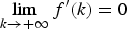
$f\lpar 0 \rpar = 0,\quad \mathop {\lim} \limits_{k \to 0} f^{\prime}\lpar k \rpar = A\alpha ^{{1 \over \sigma}} $, and $\mathop {\lim} \limits_{k \to +\infty} f^{\prime}\lpar k \rpar = 0$.


Similarly, it is easy to show the following properties of w(k t):
[3] w′(k) > 0;
[4]
$\; w\lpar 0 \rpar = 0,\quad \mathop {\lim} \limits_{k \to 0} w^{\prime}\lpar k \rpar = 0,\quad \mathop {\lim} \limits_{k \to + \infty} w^{\prime}\lpar k \rpar = 0$;[5] Define
$k^ + = \left[ { - \displaystyle{{\alpha \sigma} \over {\lpar {1 - \alpha} \rpar \lpar {1 - \sigma} \rpar }}} \right]^{ - {1 \over \sigma}}. $ Then, for $ k\gt 0,w^{\prime \prime}\lpar k \rpar \;{\gt \over \lt}\; 0 \iff k\;{\lt \over \gt}\; k^ + $.

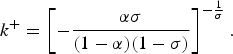

Properties [3], [4], and [5] imply that the w(k) function is S-shaped.
4.2.3. Equilibrium dynamics and steady states
Combining (26) and (27), we obtain the equilibrium dynamics of the laissez-faire economy in terms of k:
 $$k_{t + 1} = \displaystyle{\beta \over {1 + \beta}} \displaystyle{1 \over n}w\lpar {k_t} \rpar \equiv h\lpar {k_t,\; n} \rpar.$$
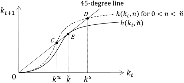
Since [β/(1 + β)](1/n) is constant for a given n, h(k t, n) is proportional to w(k t). Therefore, the shape of h(k t, n) is similar to that of the w(k t) curve. It should be noted that a rise in n rotates the h(k t, n) curve clockwise around the origin. Consequently, we define a critical value of the population growth rate,  $\check{n} , $ as shown in Figure 2, where
 $\check{n} $ is the highest population growth rate under which a steady-state equilibrium exists. From Figure 2, when
 $n = \check{n} $, the h(k t, n) curve is tangent to the 45-degree line from below. We denote the value of k at the tangent point by
 $\check{k} . $ By definition, we have
 $\partial h\lpar {\check{k} , \check{n} } \rpar /\partial k_t = 1$, and from this condition we can compute
 $\check{n} $ and
 $\check{k} $ asFootnote 9
 $$\check{n} = \displaystyle{\beta \over {1 + \beta}} A\lsqb {\alpha \lpar {1 - \sigma} \rpar } \rsqb ^{1/\sigma} \displaystyle{{ - \sigma} \over {1 - \sigma}} \gt 0,\check{k} = \left[ { - \displaystyle{{1 - \alpha} \over {\sigma \alpha}}} \right]^{1/\sigma}. $$
The graph of  $h\lpar {k_t,{\rm \;} \check{n} } \rpar $.

Now, we have the following proposition:
Proposition 3
Assume that μ = 1 and σ < 0. Then, it follows that,
(i) if
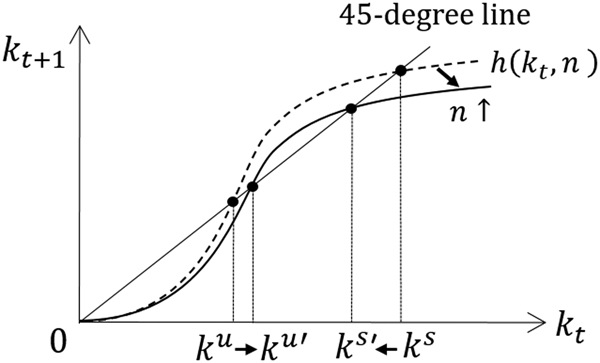
$0 \lt n \lt \check{n} $, there exist two nontrivial steady-state capital stocks k u and k s(>k u), and if $n \gt \check{n} $, no nontrivial steady state exists,(ii) when
$0 \lt n \lt \check{n}$, the lower steady-state equilibrium, k u, is unstable, while the higher steady-state equilibrium, k s, is stable.


Proof:
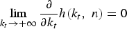
(i) In Figure 2, the h(k t, n) curve is tangent to the 45-degree line when
$n = \check{n}$ (Point E). Remember that h(k t, n) rotates counterclockwise around the origin as n decreases. Additionally, note that the slope of $h\lpar {k_t,\; n} \rpar ,\;\mathop {\lim} \limits_{k_t \to 0} \displaystyle{\partial \over {\partial k_t}}h\lpar {k_t,\; n} \rpar = 0,$ and $\mathop {\lim} \limits_{k_t \to + \infty} \displaystyle{\partial \over {\partial k_t}}h\lpar {k_t,\; n} \rpar = 0$ hold for any n because $\mathop {\lim} \limits_{k \to 0} w^{\prime}\lpar k \rpar = 0,\;\mathop {\lim} \limits_{k \to+ \infty} w^{\prime}\lpar k \rpar = 0$. Thus, for $0 \lt n \lt \check{n},$ there are two intersections of the h(k t, n) curve and the 45-degree line. On the other hand, h(k t, n) rotates clockwise around the origin as n increases; thus, for $n \gt \check{n}, $ there is no intersection.(ii) At k s and k u in Figure 3, k t+1 = h(k t, n) = k t, and thus, k remains there. Suppose that 0 < k t < k u or k s < k t. Then, the h(k t, n) curve is located below the 45-degree line, that is, k t+1 = h(k t, n) < k t, and thus, the time path of k is decreasing in this area. For k u < k t <k s, k t+1 = h(k t, n) > k t, and thus, the time path of k is increasing. From these observations, it follows that k u is unstable and k s is stable.




Two nontrivial steady states if  $0 \lt n \lt \check{n} $.

Changing n in Figure 2, we have the following corollary concerning comparative statics on the population growth rate.
Corollary
Assume that μ = 1 and σ < 0, and further  $0 \lt n \lt \check{n} $. Then, a marginal increase in n increases k u and decreases k s.
Proof:
Since an increase in n rotates the h(k t, n) curve clockwise around the origin, the result follows directly from Figure 4.
The effect of an increase in n.

4.2.4. Steady-state welfare
Since there are two steady-state equilibria for  $0 \lt n \lt \check{n} $, we must compare their welfare levels to derive the socially optimum allocation. The formula for steady-state welfare, (10), indicates that the welfare effect of a change in n depends on the signs of r − n and dk/dn. From the Corollary, we know that dk s/dn < 0 and dk u/dn > 0, and thus, it follows from (10):
 $${\rm d}U^s/{\rm d}n \;\textstyle{\gt \over \lt} \; 0 \iff r/n \;{\lt \over \gt} \; 1\,\,{\rm and}\,\,{\rm d}U^u/{\rm d}n \;{\lt \over \gt} \; 0 \iff r/n \;{\lt \over \gt} \;1,$$
where U s and U u represent steady-state utilities in the stable and unstable steady state, respectively. This result indicates that, to examine how a change in n affects steady-state utility, we should identify how a change in n affects the steady-state value of r/n.
The steady-state value of r is obtained as the solution to the following equation:
 $$\displaystyle{r \over n} = \varphi \lpar r \rpar \equiv \displaystyle{{1 + \beta} \over \beta} \displaystyle{\alpha \over {{\lpar {r/A\alpha} \rpar }^{\sigma /(1 - \sigma)} - \alpha}}. $$
The derivation of (31) is given in Appendix C. Concerning φ(r), under the assumption σ < 0, we can observe the following properties:
Properties of φ(r)
(i)
$\varphi \lpar r \rpar \gt 0\; \forall r \in \lpar {0,\; A\alpha^{1/\sigma}} \rpar $;(ii) φ′(r) > 0,
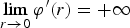
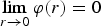
$ \;\mathop {\lim} \limits_{r \to 0} \varphi ^{\prime}\lpar r \rpar = + \infty, \;\mathop {\lim} \limits_{r \to 0} \varphi \lpar r \rpar = 0,\;\mathop {\lim} \limits_{r \to A\alpha ^{{1 \over \sigma}}} \varphi \lpar r \rpar = + \infty ;$(iii) φ(r)/r is minimized at
$\check{r} \equiv A\alpha \lsqb {\lpar {1 - \sigma} \rpar \alpha} \rsqb ^{(1 - \sigma) /\sigma}. $



Properties (i) and (ii) except for the second one are straightforwardly confirmed. Regarding the second property of (ii), differentiating φ(r) with respect to r gives
 $$\varphi ^{\prime}\lpar r \rpar = \displaystyle{{\alpha[ \lpar {1 + \beta) /\beta} ] [ { - \sigma /(1 - \sigma} \rpar] } \over {{\lsqb {{\lpar {r/A\alpha} \rpar }^{1/2\lpar {1 - \sigma} \rpar } - \alpha {\lpar {r/A\alpha} \rpar }^{(1 - 2\sigma) /2\lpar {1 - \sigma} \rpar }} \rsqb }^2}}{\rm \;}, $$
and thus, it follows that 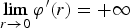 $\mathop {\lim} \limits_{r \to 0} \varphi ^{\prime}\lpar r \rpar = + \infty $. Next, consider (iii). Because
 $\varphi \lpar r \rpar /r = [(1 + \beta) /\beta] \alpha \displaystyle{1 \over {{\lpar {A\alpha} \rpar }^{ - \sigma /(1 - \sigma)} r^{1/(1 - \sigma)} - \alpha r}}$, φ(r)/r is minimized at
 $\check{r} \equiv A\alpha \lsqb {\lpar {1 - \sigma} \rpar \alpha} \rsqb ^{(1 - \sigma) /\sigma}, $ at which the denominator is maximized.
Based on properties (i) to (iii), we can depict the φ(r) curve as in Figure 5.Footnote 10 The steady-state value of r is determined by the abscissa of the intersections of two loci: the r/n locus (the straight line with 1/n slope) and the φ(r) locus. As described in subsection 4.2.2, r → 0 as k → +∞ under the assumption of σ < 0. Therefore, φ(r) is not defined at r = 0. That is, the two loci do not intersect at the origin.
The graphs of the φ(r) curve and the r/n line.
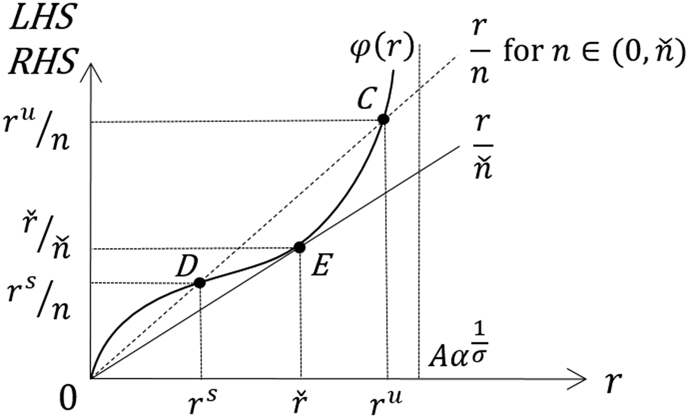
As shown in Proposition 3(i), there exist two nontrivial steady states for  $0 \lt n \lt \check{n}, $ implying that (31) has two different solutions. The dotted line in Figure 5 depicts the r/n locus for
 $n \in \lpar {0,\; \check{n} } \rpar .$ As is obvious from the figure, there are two intersection points for
 $n \in \lpar {0,\; \check{n} } \rpar $ and the values on the vertical axis of the intersection points represent the steady-state values of r/n.
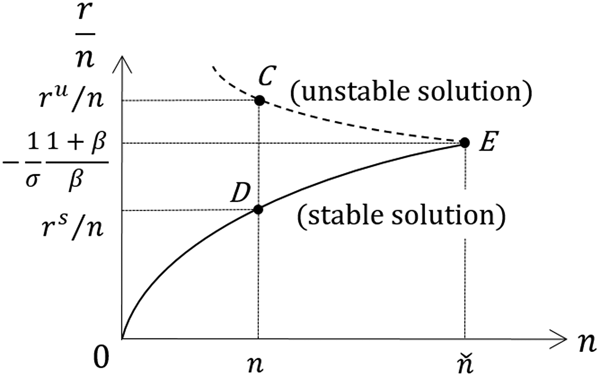
Due to the law of diminishing marginal productivity, r is negatively related to k, and the lower value of r/n, i.e., Point D in Figure 5, corresponds to a higher value of k, i.e., Point D in Figure 2, which is the stable steady state. Therefore, we denote the value of r/n in this stable steady state by r s/n. Similarly, the higher value of r/n, Point C in Figure 5, corresponds to the lower value of k, i.e., Point C, in Figure 2. Thus, Point C in Figure 5 represents the unstable steady-state equilibrium and we denote the value of r/n in the unstable steady state by r u/n.
When  $n = \check{n} $, we have a unique, nontrivial steady state. It should be noted here that Point E in Figure 5 represents the same state as Point E in Figure 2. From (27) and (29), which define
 $\check{r}$ and
 $\check{k} $, we confirm this fact and obtain
 $\check{r} / \check{n} = - \lpar {1/\sigma} \rpar {[(1 + \beta) /\beta]} $.
When  $n \gt \check{n} $, there is no nontrivial steady state as shown in Proposition 3 (i). Thus, the r/n locus and φ(r) have no intersection points.
Now, through Figure 5 we can prove the following proposition:
Proposition 4
Assume that μ = 1 and σ < 0. Then, it follows that
(i) r s/n is an increasing function of n and, r u/n is a decreasing function of n.
(ii)
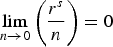
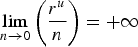
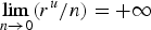
$\mathop {\lim} \limits_{n \to 0} \left( {\displaystyle{{r^s} \over n}} \right) = 0$, and $\mathop {\lim} \limits_{n \to 0} \left( {\displaystyle{{r^u} \over n}} \right) = + \infty $.(iii)
$\mathop {\lim} \limits_{n \to \check{n} } \left( {\displaystyle{{r^s} \over n}} \right) = \mathop {\lim} \limits_{n \to \check{n} } \left( {\displaystyle{{r^u} \over n}} \right) = - \displaystyle{1 \over \sigma} \displaystyle{{1 + \beta} \over \beta} $.

Proof:
(i) As n decreases, the slope of the r/n locus becomes steeper, and thus, the upper intersection of the two loci, r u/n, moves upward while the lower intersection, r s/n, moves downward. In other words, r u/n is a decreasing function of n while r s/n is an increasing function of n.
(ii) As n approaches zero, the slope of r/n locus diverges to +∞. Noting that
$\mathop {\lim} \limits_{r\to 0} \varphi ^{\prime}\lpar r \rpar = + \infty $ and $\mathop {\lim} \limits_{r\to 0} \varphi \lpar r \rpar = 0$, it is seen that Point D in Figure 5, (r s, r s/n), approaches the origin. Thus, $\mathop {\lim} \limits_{n\to 0} \lpar {r^s/n} \rpar = 0$ holds. On the other hand, because $\mathop {\lim} \nolimits_{r\to A\alpha ^{{1 \over \sigma}}} \varphi \lpar r \rpar = + \infty $, Point C (r u, r u/n) approaches (Aα 1/σ, +∞). Thus, $\mathop {\lim} \limits_{n\to 0} \lpar {r^u/n} \rpar = + \infty $ holds.(iii) As n approaches
$\check{n} $, both Points C and D converge to Point E. When $n = \check{n}, $ there is only one steady state, and the stable and unstable steady states coincide: $r^s/n = r^u/n = \check{r} /\check{n} \,\lpar { = -\lpar {1/\sigma} \rpar [\lpar {1 + \beta) /\beta} ] } \rpar $.





From Proposition 4, we can depict the relationship between n and r/n as per Figure 6. Figure 6 is obtained by changing n in Figure 5 and plotting the locus of the intersections of the φ(r) curve and the r/n line in the (n, r/n) plane. The upward-sloping curve (solid curve) indicates the relationship between n and r s/n (stable solution) while the downward-sloping curve (dashed curve) represents the relationship between n and r u/n (unstable solution). Observe that these curves intersect at  $\lpar {\check{n} , \; -\lpar {1/\sigma} \rpar {[(1 + \beta) /\beta}] } \rpar .$ The Points C, D, and E in Figure 6 correspond to Points C, D, and E in Figure 5 (and thus, in Figure 2), respectively.
The relationship between r/n and n.

We next examine whether or not the Serendipity Theorem holds by checking the stability and welfare of steady states. The critical value of r/n is 1, as (30) shows. Using Figure 6 and taking into account the location of r/n = 1 (the r/n = 1 line is drawn as a horizontal line in Figure 6 because the horizontal axis is r/n), we can derive the following proposition:
Proposition 5
Assume that σ < 0. The Serendipity Theorem holds if and only if − (1/σ)[(1 + β)/β] >1.
Proof:
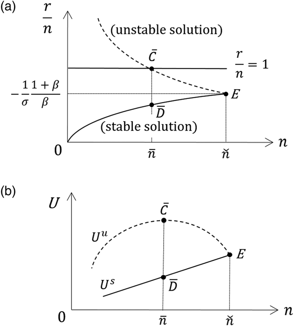
Let  $\bar{n}$ denote the population growth rate where the sideways chevron-shaped graph in Figure 6 and the r/n = 1 line intersect. Assume that −(1/σ)[(1 + β)/β] > 1. Then, the r/n = 1 line is located below Point E, and we obtain
 $\bar{n}$ as per Figure 7a. Points
 $\bar{C}$ and
 $\bar{D}$ represent the laissez-faire steady-state equilibria under
 $n = \bar{n}$, which are unstable and stable, respectively.
(a) The relationship between r/n and n in the case of − (1/σ)[(1 + β)/β] > 1. (b) The relation between U and n in the case of − (1/σ)[(1 + β)/β] > 1.
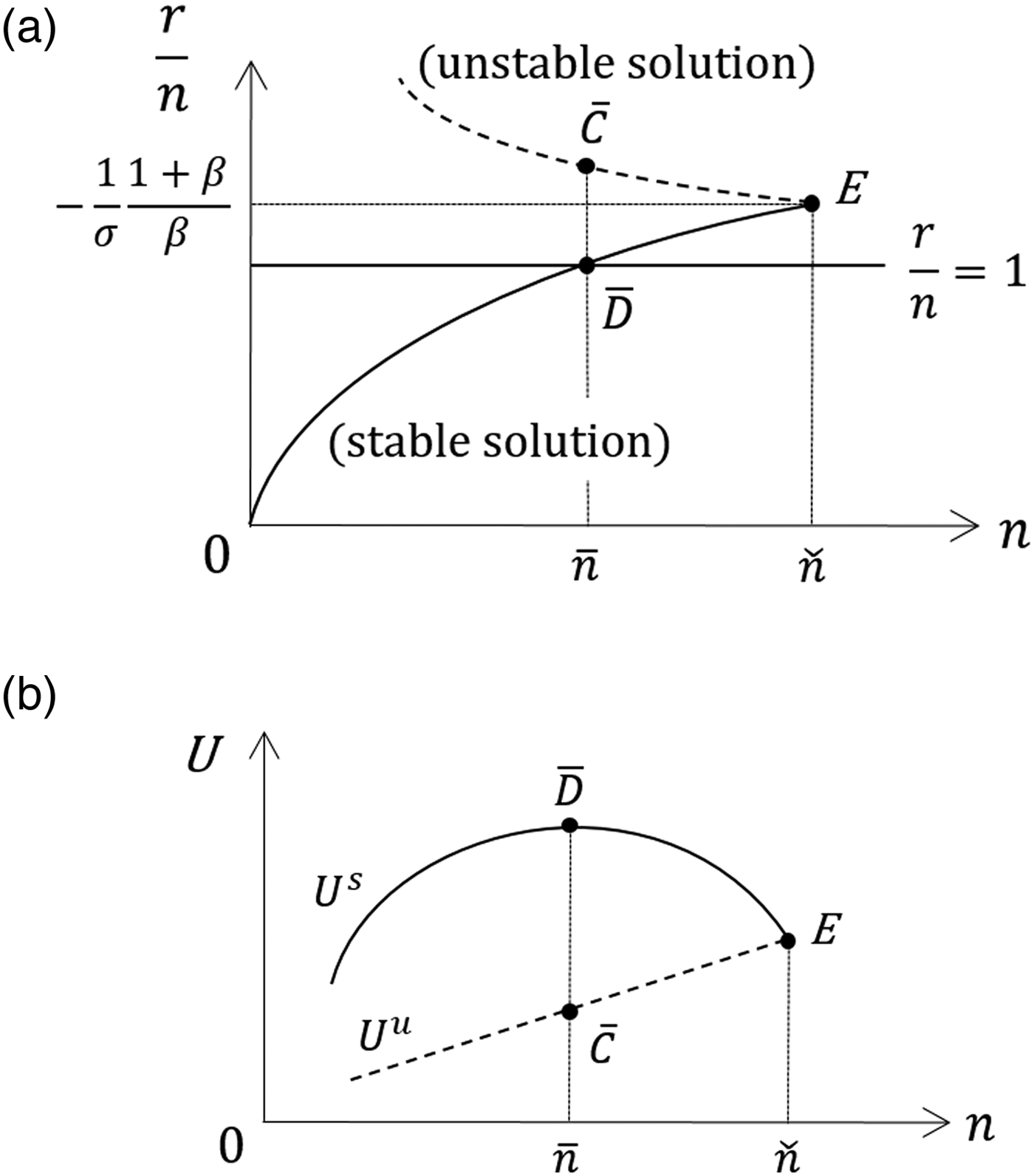
First, let us consider the upward-sloping curve passing Point  $\bar{D}$ (the solid curve). As has been stated earlier, this curve corresponds to the “stable” steady state in each n. We see that, on the upward-sloping curve, r/n <1 holds when
 $0 \lt n \lt \; \bar{n}$, and r/n >1 holds when
 ${\rm \;} \bar{n} \lt n \lt \check{n} $. Using (30), we confirm that dU s/dn > 0 when
 $0 \lt n \lt \; \bar{n}$, and dU s/dn < 0 when
 $\bar{n} \lt n \lt \check{n} $. Consequently, the relationship between n and U s is drawn as per Figure 7b.
Next, we consider the downward-sloping curve passing through Point  $\bar{C}$ (the dashed curve). This curve corresponds to the “unstable” steady state in each n. Note that r/n >1 always holds on this curve. From (30), we obtain dU u/dn > 0. Moreover, it is obvious that U s = U u when
 $n = \check{n} $. Thus, we can depict U u as per Figure 7b. Thus, Point
 $\bar{D}$ attains the highest utility among the laissez-faire steady state, and Michel and Pestieau (Reference Michel and Pestieau1993) showed that Point
 $\bar{D}$ corresponds to the MGG allocation (i.e.,
 $\; \bar{n} = n_G$). Note that Point
 $\bar{D}$ is stable, and as such, the Serendipity Theorem certainly holds in this case.
On the other hand, if − (1/σ)[(1 + β)/β] < 1, the r/n = 1 line is located above Point E and we obtain  $\bar{n}$ as per Figure 8a. Applying a similar argument to obtain Figure 7b from Figure 7a, we obtain Figure 8b from Figure 8a. We observe that Point
 $\bar{C}$ provides the highest steady-state utility; Michel and Pestieau (Reference Michel and Pestieau1993) showed that Point
 $\bar{C}$ corresponds to the MGG allocation (and again,
 $\; \bar{n} = n_G$). However, Point
 $\bar{C}$ is in the unstable region and the utility cannot be attained as a competitive equilibrium. The attainable maximum steady-state utility is provided by Point E, which is a corner solution, meaning that the Serendipity Theorem fails to hold.
(a) The relationship between r/n and n in the case of − (1/σ)[(1 + β)/β] ≤ 1. (b) The relation between U and n in the case of − (1/σ)[(1 + β)/β] ≤ 1.

5. Numerical analysis of a more general case: CES preference and CES technology
5.1. Basic setup
In subsection 4.2, to clarify the basic mechanism of our results, we restricted our attention to the case of CES technology and Cobb–Douglas preference. We showed that, if the elasticity of substitution in production is low, the MGG steady state is unstable, that is, the Serendipity Theorem fails to hold. In this section, to evaluate the realistic relevance of our analysis, we perform numerical simulations on a more general case – the case of CES preference and CES technology – by setting empirically plausible values of the key parameters.
As explained in Section 3, the MGG allocation is given by (15)–(18). Since we specify the utility and production functions to be of the CES types [see (19) and (20)], these four equations are summarized by the following two equations, the derivations of which are presented in Appendix D.
 $$A\alpha \lsqb {\lpar {1-\alpha} \rpar k_G^{-\sigma} + \alpha} \rsqb ^{(1-\sigma) /\sigma} = n_G,$$
 $$\alpha \lsqb {\beta^{-\mu} n_G^{1-\mu} + 1} \rsqb = \lpar {1-\alpha} \rpar k_G^{-\sigma}. $$
From (32) and (33) we can solve for k G and n G. Since the elasticity of substitution in production, 1/(1 − σ), is directly estimated in the empirical literature, it is convenient to introduce a new variable representing the elasticity of substitution in production, τ ≡ 1/(1 − σ). Using τ, we can rewrite (32) and (33) as:
 $$A\alpha = n_G\lsqb {\lpar {1-\alpha} \rpar k_G^{(1-\tau) /\tau} + \alpha} \rsqb ^{1/(1-\tau)}, $$
 $$\alpha \lsqb {\beta^{-\mu} n_G^{1-\mu} + 1} \rsqb = \lpar {1-\alpha} \rpar k_G^{(1-\tau) /\tau}. $$
In our numerical simulations, we restrict our attention to the case of 0 < τ < 1 ( ⇔ σ < 0) and 0 < μ < 1, under which an MGG allocation exists, as proved by Michel and Pestieau (Reference Michel and Pestieau1993).Footnote 11
The marginal propensity to save and the wage and gross interest rate under the double CES assumption are given by:
 $$\theta \lpar {r_{t + 1}} \rpar \equiv \beta ^{-\mu} \cdot (r_{t + 1})^{1-\mu} + 1$$
 $$\eqalign{& w_t = w\lpar {k_t} \rpar = A\lpar {1-\alpha} \rpar \lsqb {\lpar {1-\alpha} \rpar + \alpha k_t^{-(1-\tau) /\tau}} \rsqb ^{-1/(1-\tau)}, {\rm \;} \cr & r_t = r\lpar {k_t} \rpar = A\alpha \lsqb {\lpar {1-\alpha} \rpar k_t^{(1-\tau) /\tau} + \alpha} \rsqb ^{-1/(1-\tau)}.} $$
We can express the equilibrium dynamics when the population growth rate is set at n G as:
 $$H\lpar {k_t,\; k_{t + 1}} \rpar \equiv w\lpar {k_t} \rpar -n_Gk_{t + 1}\lpar {\beta^{-\mu} \cdot r{\lpar {k_{t + 1}} \rpar }^{1-\mu} + 1} \rpar = 0,$$
which is derived from (9) and (36). When k t = k t+1 = k G, H(k G, k G) = 0, and thus the MGG allocation constitutes a steady-state laissez-faire equilibrium under the population growth rate n G. This is a restatement of the result of Samuelson (Reference Samuelson1975). It should be noted here that this does not mean that the MGG steady state is the unique steady state; there may be multiple steady states.
In order to check the local stability of the MGG steady state, k t = k t+1 = k G, we evaluate the following value:
 $$\left. {\displaystyle{{{\rm d}k_{t + 1}} \over {{\rm d}k_t}}} \right \vert _{k_t = k_{t + 1} = k_G} = -\displaystyle{{\partial H\lpar {k_G,\; k_G} \rpar } \over {\partial k_t}}/\displaystyle{{\partial H\lpar {k_G,\; k_G} \rpar } \over {\partial k_{t + 1}}}.$$
If the absolute value of  $ {{\rm d}k_{t + 1}/{\rm d}k_t} \vert _{k_t = k_{t + 1} = k_G}$ is greater than unity, then the MGG steady state is locally unstable, and thus, the Serendipity Theorem fails to hold.
Regarding (38), we obtain the following lemma.
Lemma 1
When τ = μ = 0.5, it always holds that  $ {{\rm d}k_{t + 1}/{\rm d}k_t} \vert _{k_t = k_{t + 1} = k_G} = 1$, regardless of the values of A, α, and β.
The proof is given in Appendix E. Lemma 1 indicates that, when τ = μ = 0.5, a tangent bifurcation occurs at the MGG steady state. That is, the MGG steady state is represented as Point E in Figure 2, regardless of the values of A, α, and β.
5.2. Numerical simulations
5.2.1. Choice of parameter values
We briefly explain our choice of values of structural parameters, α, β, δ, A, τ, and μ. We begin with δ, α, and A.
Since our overlapping generations model consists of two periods, the length of one period could be reasonably considered to be about 30 years; thus, the depreciation rate would be large. Following de la Croix and Doepke (Reference de la Croix and Doepke2003), who performed similar numerical simulations of a two-period overlapping generations model, we assume that the capital entirely depreciates after one period, that is, δ = 1. Moreover,we specify α = 0.4. Under this value, the steady-state labor income is computed as 0.6–0.7, consistent with most empirical estimates of the labor income share.Footnote 12 Following de la Croix and Doepke (Reference de la Croix and Doepke2003), the benchmark value of the productivity parameter, A, is set at unity. In subsection 5.2.4, we examine the robustness of our numerical simulation results by changing the value of A.
We next observe the range of β. Several studies have constructed the value of β by following the business cycle literature, which often employs 0.99 as the per quarter discount factor. When we apply this discount rate to our economy, we set β = 0.3 because (0.99)4×30 ≈ 0.3.Footnote 13 Moreover, we report the case of β = 1 in order to check how changes in β affect the stability of the MGG steady state.Footnote 14
The elasticity of substitution in production, τ, and the degree of intertemporal substitution, μ, may be controversial because the estimated values of τ and μ have a wide range. Chirinko (Reference Chirinko2008) stated that evidence suggests that the elasticity of substitution in production, τ, ranges from 0.40 to 0.60, while Klump et al. (Reference Klump, McAdam and Willman2008) obtained 0.7 as the elasticity of substitution in production, τ. Based on these results, this paper specifies that τ lies within the range [0.4, 0.7].Footnote 15
Concerning intertemporal substitution μ, Table 1 of Havránek et al. (Reference Havránek, Horvath, Iršová and Rusnak2015), which summarizes individual countries’ estimated value of intertemporal substitution for 45 countries, shows a very wide range of estimated values of μ. Given that two-thirds of the mean elasticities lie in the range [0.1, 0.7], we consider this to be the range of μ.Footnote 16
5.2.2. Stability of the MGG steady state
First, given β = 0.3, A = 1, and α = 0.3 (we call this the benchmark case), we examine the relationship between the stability of the MGG steady state and the two key parameters, τ and μ. Figure 9 depicts the stable region, where  $0 \lt {{\rm d}k_{t + 1}/{\rm d}k_t} \vert _{k_t = k_{t + 1} = k_G} \lt 1$, and the unstable region, where
 $ {{\rm d}k_{t + 1}/{\rm d}k_t} \vert _{k_t = k_{t + 1} = k_G} \gt 1$, in the τ − μ plane. The solid curve represents the locus that satisfies
 $ {{\rm d}k_{t + 1}/{\rm d}k_t} \vert _{k_t = k_{t + 1} = k_G} = 1$, that is, the border of the two regions. The key results are: the border is downward sloping, and the MGG steady state is unstable when τ and μ take small values.Footnote 17 Furthermore, the border passes through (0.5, 0.5), as Lemma 1 shows. Through a numerical examination, under our parameter settings, we confirm that the graph of the dynamical system, H(k t, k t+1) = 0, is expressed as an S-shaped curve, such as in Figure 3.
Benchmark case (A = 1, β = 0.3, α = 0.3).

Next, let us examine how changes in the value of β affect the result. We change the value of β from 0.3 to 1 (the other parameters are fixed at the benchmark values), and consider how the border changes. Figure 10 depicts the result. The dashed and solid curves represent the border in the benchmark case (the same as Figure 9), and the high β case, respectively. Again, the border is downward sloping and passes through (0.5, 0.5). We observe that the unstable region expands for 0.4 < τ < 0.5, while it shrinks for 0.5 < τ. This suggests that, in a country where the elasticity of substitution in production is low, a higher propensity to save tends to make the MGG steady state unstable.
Effect of an increase in β.

Finally, let us examine how changes in the value of A affect the unstable region. Here, we change the value of A from 1 to 5 (the other parameters are fixed at the benchmark values). The result is depicted in Figure 11.
Effect of an increase in A.
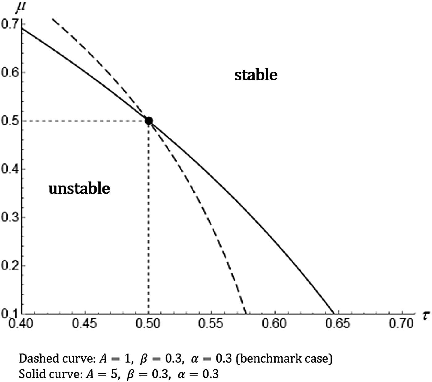
The dashed and solid curves represent the border in the benchmark case (the same as Figure 9), and the high A case, respectively. Figure 11 shows that, the MGG steady state is unstable when τ and μ take small values, in the same way as Figures 9 and 10, and that, an increase in A makes the unstable region smaller for 0.4 < τ < 0.5, while it expands the unstable region for 0.5 < τ. This implies that, in an economy where the elasticity of substitution in production is low, an improvement in the TFP tends to stabilize the MGG steady state.
5.3. Policy implications: a potential pitfall
We confirmed that the MGG steady state is unstable when τ and μ take small values, and thus, the Serendipity Theorem can fail to hold under empirically plausible parameter values. We argue that this has significant policy implications.
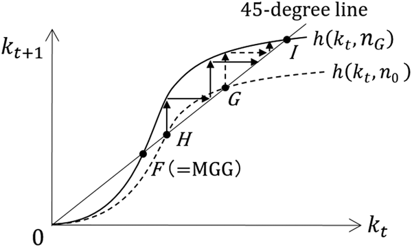
Assume that the MGG steady state is unstable. In this case, the MGG steady state corresponds to Point C in Figure 3, and this scenario follows that in Figure 8b. Suppose that the population growth rate is n 0(>n G), as in Figure 12. If the government does not take into consideration the stability issue and believes that the Serendipity Theorem is applicable, it decreases the population growth rate to n G by expecting the economy to move from Point H to Point F. However, Point H is an unstable steady state, and thus, it is natural to assume that the economy is initially located at Point G. Therefore, this policy will move the economy from Point G to Point I (refer to the dotted arrows in Figure 13). As a result, steady-state welfare deteriorates, contrary to the government's intention (see Figure 12). Moreover, if the economy is at Point H (the unstable steady state), changing the population growth rate from n 0 to n G causes the economy to move from Point H to Point I (refer to the solid arrows in Figure 13). In this case, social welfare decreases to a greater degree than in the previous situation (see Figure 12).
A potential pitfall (case of − (1/σ) ((1 + β)/β) ≤ 1 and n0 > nG).

Wrong policy (n0 > nG).

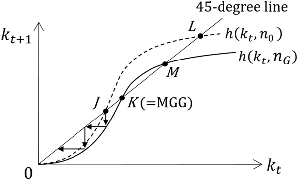
Let us consider another example. Assume that in the situation in Figure 8b the population growth rate is given by n 0(<n G), as depicted in Figures 14 and 15, and that the economy is in the lower unstable steady state, Point J. If the government believes that it can apply the Serendipity Theorem, it will increase the population growth rate to n G by expecting that the economy moves from Point J to K (see Figure 14). However, once n is increased, the economy moves toward the origin (refer to the solid arrows in Figure 15). As a result, the economy shrinks and welfare deteriorates, contrary to the government's intention.
A potential pitfall (case of − (1/σ) ((1 + β)/β) ≤ 1 and n0 < nG).

Wrong policy (n0 < nG).

These examples indicate the importance of the stability consideration in analyzing the Serendipity Theorem.
6. Concluding remarks
We reexamined the Serendipity Theorem of Samuelson (Reference Samuelson1975) from the stability viewpoint. Specifically, we investigated whether the MGG allocation can be supported by the stable steady-state competitive equilibrium. Moreover, we showed that, in the case of Cobb–Douglas preference and CES technology, the stability of the MGG lifetime state depends on parameter values and, in some situations, the Serendipity Theorem fails to hold despite steady-state welfare being maximized at the population growth rate as the steady state is unstable. Furthermore, using numerical simulations, we investigated a more general case, specifically that of CES preference and CES technology, and showed that the MGG lifetime state is unstable when the elasticities of substitution in consumption and production are small. These form the main contributions of this paper given that the previous studies on the Serendipity Theorem have not analyzed the stability issue in detail.
Supplementary material
The supplementary material for this article can be found at https://doi.org/10.1017/dem.2018.21.
Author ORCIDs
Akira Momota, 0000-0002-3363-7417.
Acknowledgements
The authors would like to thank the two anonymous referees and the editor, David de la Croix, as well as Masakatsu Okubo and seminar participants at Kyoto University, for their helpful comments and suggestions. This study was financially supported by the joint research program of KIER and Grants-in-Aid for Scientific Research from the JSPS (grant numbers 25380221, 18K01524, 16H03631, and 17H02516).
Appendix A
In this appendix, we derive the welfare evaluation formula (10). Differentiating U(c, d) with respect to n gives
 $$\displaystyle{{{\rm d}U} \over {{\rm d}n}} = U_c\lpar {c,d} \rpar \displaystyle{{{\rm d}c} \over {{\rm d}n}} + U_d\lpar {c,d} \rpar \displaystyle{{{\rm d}d} \over {{\rm d}n}}\;.$$
Substituting (6) into (A.1), we have
 $$\displaystyle{{{\rm d}U} \over {{\rm d}n}} = U_c\left( {\displaystyle{{{\rm d}c} \over {{\rm d}n}} + \displaystyle{1 \over r}\displaystyle{{{\rm d}d} \over {{\rm d}n}}} \right).$$
From (4), (5), and the equilibrium condition of the economy, (9), we have
 $$\displaystyle{{{\rm d}c} \over {{\rm d}n}} = \displaystyle{{{\rm d}\lpar {w-s} \rpar } \over {{\rm d}n}} = \displaystyle{{{\rm d}w} \over {{\rm d}n}}-k-n\displaystyle{{{\rm d}k} \over {{\rm d}n}},$$
 $$\displaystyle{{{\rm d}d} \over {{\rm d}n}} = \displaystyle{{{\rm d}\lpar {rnk} \rpar } \over {{\rm d}n}} = \displaystyle{{{\rm d}r} \over {{\rm d}n}}nk + rn\displaystyle{{{\rm d}k} \over {{\rm d}n}} + rk.$$
Thus, substituting (A.3) and (A.4) into (A.2) we obtain
 $$\displaystyle{{{\rm d}U} \over {{\rm d}n}} = \; U_c\left( {\displaystyle{{{\rm d}w} \over {{\rm d}n}} + \displaystyle{{nk} \over r}\displaystyle{{{\rm d}r} \over {{\rm d}n}}} \right) = \; U_c\left( {\displaystyle{{{\rm d}w} \over {{\rm d}k}} + \displaystyle{{nk} \over r}\displaystyle{{{\rm d}r} \over {{\rm d}k}}} \right)\displaystyle{{{\rm d}k} \over {{\rm d}n}}.$$
Finally, substituting the derivatives of w and r in (3) with respect to k into (A.5), we have the following formula for welfare evaluation:
 $$\displaystyle{{{\rm d}U} \over {{\rm d}n}} = \; U_c(c,d)\lpar {-kf^{\prime \prime}(k)} \rpar \displaystyle{1 \over r}\lpar {r-n)} \rpar \displaystyle{{{\rm d}k} \over {{\rm d}n}}.$$
Appendix B
This appendix derives (29) of the main text. As per Figure 3, when  $n = \check{n} $, the h(k t, n) curve is tangent to the 45-degree line. We denote the value of k at the tangent point by
 $\check{k} , \; $ that is,
 $$h_k\lpar {\check{k}, \check{n}} \rpar = 1,$$
where h k denotes the partial derivative of h with respect to k. As per Figure 3, at the tangent point, the following relation holds:
 $$\displaystyle{{h\lpar {\check{k}, \check{n}} \rpar } \over {\check{k}}} = h_k\lpar {\check{k}, \check{n}} \rpar .$$
Since 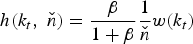 $h\lpar {k_t,\; \check{n} } \rpar = \displaystyle{\beta \over {1 + \beta}} \displaystyle{1 \over {\check{n} }} w\lpar {k_t} \rpar $, this is equivalent to
 $$\displaystyle{{w\lpar {\check{k}} \rpar } \over {\check{k}}} = w^{\prime}\lpar {\check{k}} \rpar ,$$
from which we can solve  $\check{k}$ as follows:
 $$\check{k} = \left[ {-\displaystyle{{1-\alpha} \over {\sigma \alpha}}} \right]^{1/\sigma}.$$
Substituting this into (B.1), we have
 $$h_k\lpar {\check{k}, \check{n}} \rpar = \displaystyle{1 \over {\check{n}}} \displaystyle{\beta \over {1 + \beta}} A\lsqb {\alpha \lpar {1-\sigma} \rpar } \rsqb ^{1/\sigma} \displaystyle{{-\sigma} \over {1-\sigma}} = 1.$$
From this equation, we obtain
 $$\check{n} = \displaystyle{\beta \over {1 + \beta}} A\lsqb {\alpha \lpar {1-\sigma} \rpar } \rsqb ^{1/\sigma} \displaystyle{{-\sigma} \over {1-\sigma}}. $$
Appendix C
In this appendix, we derive (31). First, we prove the following lemma.
Lemma 2
 $$\displaystyle{{w\lpar k \rpar } \over k} = A^{-{\sigma \over {1-\sigma}}} \alpha ^{-{1 \over {1-\sigma}}} r\lpar k \rpar ^{{1 \over {1-\sigma}}} -r\lpar k \rpar .$$
Proof:
From (27), we have
 $$\displaystyle{{w\lpar k \rpar } \over k} = \displaystyle{{\,f\lpar k \rpar } \over k}-r\lpar k \rpar.$$
Since capital income is represented as
 $$\displaystyle{{r\lpar k \rpar k} \over {\,f\lpar k \rpar }} = \displaystyle{\alpha \over {\lpar {1-\alpha} \rpar k^{-\sigma} + \alpha}} \;, $$
we have
 $$\displaystyle{{\,f\lpar k \rpar } \over k} = \displaystyle{{r\lpar k \rpar } \over \alpha} \lsqb {\lpar {1-\alpha} \rpar k^{-\sigma} + \alpha} \rsqb .$$
Using the equality between the interest rate and marginal productivity of capital, we can rewrite (C.2) as
 $$\displaystyle{{\,f\lpar k \rpar } \over k} = \displaystyle{{r\lpar k \rpar } \over \alpha} \left( {\displaystyle{{r\lpar k \rpar } \over {A\alpha}}} \right)^{\sigma /(1-\sigma)} = A^{-\sigma /(1-\sigma)} \alpha ^{-1/(1-\sigma)} r\lpar k \rpar ^{1/(1-\sigma)}.$$
Substituting (C.3) into (C.1), we have
 $$\displaystyle{{w\lpar k \rpar } \over k} = A^{-\sigma /(1-\sigma)} \alpha ^{-1/(1-\sigma)} r\lpar k \rpar ^{1/(1-\sigma)} -r\lpar k \rpar .$$
Let us next consider the steady state of (26), that is,
 $$nk = \displaystyle{\beta \over {1 + \beta}} w(k).$$
If k ≠ 0, this can be expressed as
 $$n = \displaystyle{\beta \over {1 + \beta}} \displaystyle{{w\lpar k \rpar } \over k}.$$
Using Lemma 2, we can rewrite (C.4) as follows:
 $$n = \displaystyle{\beta \over {1 + \beta}} \lsqb {A^{-\sigma /(1-\sigma)} \alpha^{-1/(1-\sigma)} r{\lpar k \rpar }^{1/(1-\sigma)} -r\lpar k \rpar } \rsqb .$$
Since  $\sigma \lt 0,\quad \mathop {\lim} \limits_{k\to + \infty} r\lpar k \rpar = 0$, and hence, r ≠ 0 holds for all 0 <k < + ∞. Dividing both sides of (C.5) by r and taking their reciprocals, we have
 $$\displaystyle{r \over n} = \displaystyle{{1 + \beta} \over \beta} \displaystyle{\alpha \over {{\lpar {r/A\alpha} \rpar }^{\sigma /(1-\sigma)} -\alpha}} \;. $$
Therefore, we have derived (31) in the main text.
Appendix D This appendix derives (32) and (33). Under the double CES assumption, (15) and (16) are given by
 $$A\alpha \lsqb {\lpar {1-\alpha} \rpar + \alpha k_G^\sigma} \rsqb ^{(1-\sigma) /\sigma} k_G^{\sigma -1} = n_G,$$
and
 $$c_G = \beta ^{-\mu} n_G^{-\mu} d_G.$$
(32) directly follows (D.1). From (17), (18), and (D.2), we have
 $$A\lsqb {\lpar {1-\alpha} \rpar + \alpha k_G^\sigma} \rsqb ^{1/\sigma} = n_Gk_G\lsqb {\beta^{-\mu} \cdot n_G^{1-\mu} + 2} \rsqb .$$
Appendix E Lemma 1 is proved here. We first solve k G and n G for τ = μ = 0.5 (σ = −1). In this case, (34) and (35) are given by
 $$A\alpha = n_G\lsqb {\lpar {1-\alpha} \rpar k_G + \alpha} \rsqb ^2, {\rm and} $$
 $$\alpha \lsqb {\beta^{-1/2}n_G^{1/2} + 1} \rsqb = \lpar {1-\alpha} \rpar k_G\;.$$
Deleting k G from (E.1) and (E.2), we obtain
 $$\displaystyle{A \over \alpha} = \lsqb {\beta^{-1/2}n_G + 2n_G^{1/2}} \rsqb ^2\;. $$
Noting that β −1/2n + 2n 1/2 >0 and defining z ≡ n 1/2, (E.3) is transformed into the following quadratic equation of z:
 $$\beta ^{-1/2}z^2 + 2z = \left( {\displaystyle{A \over \alpha}} \right)^{1/2}.$$
Since z must be positive, the solution to this equation is given by
 $$z = n_G^{1/2} = \displaystyle{{\sqrt {1 + {\lpar {A/\alpha \beta} \rpar }^{1/2}} -1} \over {\beta ^{-1/2}}}\;,$$
indicating that
 $$n_G = \beta \left( {\sqrt {1 + {\left( {\displaystyle{A \over {\alpha \beta}}} \right)}^{1/2}} -1} \right)^2\;. $$
Moreover, from (E.2) and (E.4), k G is obtained as
 $$k_G = \displaystyle{\alpha \over {1-\alpha}} \sqrt {1 + {\left( {\displaystyle{A \over {\alpha \beta}}} \right)}^{1/2}} \;. $$
We next derive the dynamics of the laissez-faire equilibrium for the case of τ = μ = 0.5 and n = n G. From (36) and (37), we have
 $$H\lpar {k_t,\; k_{t + 1}} \rpar \equiv A\lpar {1-\alpha} \rpar \lsqb {\lpar {1-\alpha} \rpar + \alpha k_t^{-1}} \rsqb ^{-2}-n_Gk_{t + 1}\left\{ {{\left( {\displaystyle{{A\alpha} \over \beta}} \right)}^{1/2}{\lsqb {\lpar {1-\alpha} \rpar k_{t + 1} + \alpha} \rsqb }^{-1} + 1} \right\} = 0\;.$$
Partially differentiating (E.7) with respect to k t, we have
 $$\eqalign{\displaystyle{{\partial H\lpar {k_G,\; k_G} \rpar } \over {\partial k_t}} &= \displaystyle{{2A\lpar {1-\alpha} \rpar \alpha} \over {{\lsqb {\lpar {1-\alpha} \rpar + \alpha k_G^{-1}} \rsqb }^3\cdot k_G^2}} = \displaystyle{{2A\lpar {1-\alpha} \rpar \alpha} \over {{\lsqb {\lpar {1-\alpha} \rpar + \alpha k_G^{-1}} \rsqb }^2\cdot k_G^2}} \cdot \displaystyle{1 \over {\lpar {1-\alpha} \rpar + \alpha k_G^{-1}}} \cr & = \displaystyle{{2A\lpar {1-\alpha} \rpar \alpha} \over {{\lsqb {\lpar {1-\alpha} \rpar k_G + \alpha} \rsqb }^2}}\cdot \displaystyle{1 \over {\lpar {1-\alpha} \rpar + \alpha k_G^{-1}}} \;.}$$
Substituting (E.1) into the first term of the right-hand side of the above equation yields
 $$\displaystyle{{\partial H\lpar {k_G,\; k_G} \rpar } \over {\partial k_t}} = 2\lpar {1-\alpha} \rpar n_G\cdot \displaystyle{1 \over {\lpar {1-\alpha} \rpar + \alpha k_G^{-1}}} {\rm \;} = 2\lpar {1-\alpha} \rpar n_G\cdot \displaystyle{{k_G} \over {\lpar {1-\alpha} \rpar k_G + \alpha}}$$
As (E.1) and (E.2) can be rewritten as
 $$\left( {\displaystyle{{A\alpha} \over {n_G}}} \right)^{1/2} = \lpar {1-\alpha} \rpar k_G + \alpha, $$
and
 $$\left( {\displaystyle{{n_G} \over \beta}} \right)^{1/2} = \displaystyle{{\lpar {1-\alpha} \rpar k_G-\alpha} \over \alpha},$$
respectively, we obtain the following equation by combining (E.9) and (E.10):
 $$\left( {\displaystyle{{A\alpha} \over \beta}} \right)^{1/2} = \displaystyle{{\lsqb {\lpar {1-\alpha} \rpar k_G + \alpha} \rsqb \cdot \lsqb {\lpar {1-\alpha} \rpar k_G-\alpha} \rsqb } \over \alpha}.$$
Partially differentiating (E.7) with respect to k t+1, we obtain
 $$\eqalign{\displaystyle{{\partial H\lpar {k_G,\; k_G} \rpar } \over {\partial k_{t + 1}}} = &-n_G\left\{ {{\left( {\displaystyle{{A\alpha} \over \beta}} \right)}^{1/2}\displaystyle{1 \over {\lpar {1-\alpha} \rpar k_G + \alpha}} + 1-k_G{\left( {\displaystyle{{A\alpha} \over \beta}} \right)}^{1/2}\lpar {1-\alpha} \rpar \displaystyle{1 \over {{\lpar {\lpar {1-\alpha} \rpar k_G + \alpha} \rpar }^2}}} \right\} \cr = &-n_G\left\{ {1 + {\left( {\displaystyle{{A\alpha} \over \beta}} \right)}^{1/2}\displaystyle{\alpha \over {{\lpar {\lpar {1-\alpha} \rpar k_G + \alpha} \rpar }^2}}} \right\}.} $$
Substituting (E.11) into the right-hand side of the above equation, we have
 $$\displaystyle{{\partial H\lpar {k_G,\; k_G} \rpar } \over {\partial k_{t + 1}}} = -n_G\left( {1 + \displaystyle{{\lpar {1-\alpha} \rpar k_G-\alpha} \over {\lpar {1-\alpha} \rpar k_G + \alpha}}} \right) = -n_G\displaystyle{{2\lpar {1-\alpha} \rpar k_G} \over {\lpar {1-\alpha} \rpar k_G + \alpha}}.$$
Finally, substituting (E.8) and (E.12) into (38), we obtain
 $$\left. {\displaystyle{{{\rm d}k_{t + 1}} \over {{\rm d}k_t}}} \right \vert _{k_t = k_{t + 1} = k_G} = -\displaystyle{{\partial H\lpar {k_G,\; k_G} \rpar } \over {\partial k_t}}/\displaystyle{{\partial H\lpar {k_G,\; k_G} \rpar } \over {\partial k_{t + 1}}} = 1.$$
Thus,  $ {{\rm d}k_{t + 1}/{\rm d}k_t} \vert _{k_t = k_{t + 1} = k_G} = 1$, regardless of the values of A, α, and β.