1 Introduction
In linear water wave theory, the landslide movement is modelled as an external forcing function and the thickness of the landslide is assumed to be small relative to the water depth due to linearisation. For the simplest situation, i.e. the one-dimensional (horizontal) linear shallow water equations (1DH LSWEs) in constant water depth, the dimensionless mass and momentum equations are
 $$\begin{eqnarray}\displaystyle \unicode[STIX]{x1D702}_{t}+u_{x}=B_{t} & & \displaystyle\end{eqnarray}$$
and
 $$\begin{eqnarray}\displaystyle u_{t}=-\unicode[STIX]{x1D702}_{x}, & & \displaystyle\end{eqnarray}$$
where
 $\unicode[STIX]{x1D702}(x,t)$
is the free-surface elevation,
 $B(x,t)$
is the landslide forcing function and
 $u(x,t)$
is the horizontal velocity. Equations (1.1) and (1.2) can be combined to solve for either
 $\unicode[STIX]{x1D702}$
or
 $u$
first. Solving for
 $\unicode[STIX]{x1D702}$
only, Tinti, Bortolucci & Chiavettieri (Reference Tinti, Bortolucci and Chiavettieri2001) have shown that the dimensionless analytical solution for waves generated by a solid landslide moving at a constant speed is simply
 $$\begin{eqnarray}\displaystyle \left.\begin{array}{@{}c@{}}\displaystyle \unicode[STIX]{x1D702}(x,t)=\unicode[STIX]{x1D702}_{_{Fr}}(x,t)+\unicode[STIX]{x1D702}_{+}(x,t)+\unicode[STIX]{x1D702}_{-}(x,t),\\ \displaystyle \unicode[STIX]{x1D702}_{_{Fr}}(x,t)=-\frac{Fr^{2}}{1-Fr^{2}}B(x-Fr\,t),\\ \displaystyle \unicode[STIX]{x1D702}_{+}(x,t)=\frac{Fr}{2(1-Fr)}B(x-t),\\ \displaystyle \unicode[STIX]{x1D702}_{-}(x,t)=-\frac{Fr}{2(1+Fr)}B(x+t),\end{array}\right\} & & \displaystyle\end{eqnarray}$$
where
 $B(x,t)=B(x-Fr\,t)$
is the prescribed landslide forcing function and
 $Fr$
, defined as the Froude number, is the constant landslide speed normalised by the constant linear wave speed. The velocity solution can be recovered from the momentum equation (1.2) as
 $$\begin{eqnarray}\displaystyle \left.\begin{array}{@{}c@{}}\displaystyle u(x,t)=u(x,0)+u_{_{Fr}}(x,t)+u_{+}(x,t)+u_{-}(x,t),\\ \displaystyle u_{_{Fr}}(x,t)=-\frac{Fr}{1-Fr^{2}}B(x-Fr\,t),\\ \displaystyle u_{+}(x,t)=\frac{Fr}{2(1-Fr)}B(x-t),\\ \displaystyle u_{-}(x,t)=\frac{Fr}{2(1+Fr)}B(x+t).\end{array}\right\} & & \displaystyle\end{eqnarray}$$
In solving (1.1) and (1.2) for
 $\unicode[STIX]{x1D702}$
, the imposed initial conditions are
 $\unicode[STIX]{x1D702}(x,0)=0$
and
 $\unicode[STIX]{x1D702}_{t}(x,0)=B_{t}(x,0)$
; the second condition results from setting
 $u_{x}(x,0)=0$
in (1.1). Thus, the solution for
 $\unicode[STIX]{x1D702}$
, equation (1.3), is valid for any initial flow set-up with initial conditions
 $\unicode[STIX]{x1D702}(x,0)=0$
and
 $u(x,0)=\text{const}$
. The precise initial velocity
 $u(x,0)$
can be specified only when the solution for
 $u$
is considered; for initially quiescent water, one requires
 $u(x,0)=0$
in (1.4).
The solution (1.3) reflects the three-wave structure of waves generated by a moving landslide – the two free waves
 $\unicode[STIX]{x1D702}_{+}$
and
 $\unicode[STIX]{x1D702}_{-}$
that travel at wave celerity in opposite directions and a trapped wave
 $\unicode[STIX]{x1D702}_{_{Fr}}$
that follows the landslide. In addition to the sign difference, the magnitude of the right-going wave,
 $\unicode[STIX]{x1D702}_{+}$
, is always larger than that of the left-going wave,
 $\unicode[STIX]{x1D702}_{-}$
, and the difference is especially significant for
 $Fr\sim 1$
, when resonance occurs. Tinti & Bortolucci (Reference Tinti and Bortolucci2000) showed that the resonance solution (
 $Fr=1$
) for the 1DH LSWEs can be obtained by the method of characteristics:
 $$\begin{eqnarray}\displaystyle \unicode[STIX]{x1D702}(x,t)=\frac{t}{2}B_{t}(x-t)+\frac{1}{4}B(x-t)-\frac{1}{4}B(x+t). & & \displaystyle\end{eqnarray}$$
In the resonance case, the right-going wave grows linearly in time and its form also depends on the first temporal derivative of the landslide forcing function.
Analytical solutions are also possible for other wave models and more complex water depth or landslide configurations. Applying the Laplace and Fourier transformation methods to the linear and fully dispersive wave model in constant water depth, Mei (Reference Mei1989) derived the general solution for waves generated by a seafloor displacement as well as the asymptotic far-field leading-wave solutions for specific bottom displacement functions. By using the Laplace and Hankel transforms, Tuck & Hwang (Reference Tuck and Hwang1972) first derived the general integral-form solution (consisting of three integrals) to the 1DH LSWEs for landslide-generated waves on a constant slope. Liu, Lynett & Synolakis (Reference Liu, Lynett and Synolakis2003) found that by choosing a deforming Gaussian-like landslide accelerating at the same rate as the local wave celerity (wave celerity increases as water depth increases), the integral-form solution can be simplified so that only one integral needs to be numerically evaluated. Didenkulova et al. (Reference Didenkulova, Nikolkina, Pelinovsky and Zahibo2010) and Didenkulova, Nikolkina & Pelinovsky (Reference Didenkulova, Nikolkina and Pelinovsky2011) also found simplified solutions based on the 1DH LSWEs for water waves generated by a deforming submarine landslide on a convex slope, and examined resonance more closely.
Extending the landslide-wave problem to two horizontal dimensions, Sammarco & Renzi (Reference Sammarco and Renzi2008) and Renzi (Reference Renzi2010) derived the general integral-form landslide-wave solution (consisting of three integrals and a series) for the two-dimensional (horizontal) (2DH) LSWEs on a plane beach, and examined the large-time asymptotic behaviour of the generated waves. The same solution process was later used to study landslide-generated waves around a conical island (Renzi & Sammarco Reference Renzi and Sammarco2010) and the effects of landslide shape in LSWEs (Renzi & Sammarco Reference Renzi and Sammarco2012). Seo & Liu (Reference Seo and Liu2013) extended the solution process to allow for more arbitrary landslide shapes and placed a stronger emphasis on the numerical integration methods.
In this study, we seek to further contribute to analytical solutions on landslide-generated water waves. For a solid landslide moving at a constant speed in constant water depth, we derive 1DH analytical solutions for the linear and weakly dispersive model as well as the linear and fully dispersive model, which clearly display the three-wave structure, as expected. Using the linear and fully dispersive model in constant depth, we show that the area enclosed by the landslide has the strongest lasting effects on the generated waves, and that the exact landslide shape is irrelevant to the leading order. In addition, we also examine the resonance solution using the same model.
For landslide-generated waves on a constant slope, we present a closed-form analytical solution in 1DH by using a special landslide forcing function. The analytical solution consists of a ‘shoreline’ in linear theory and a travelling shock, and can therefore serve as a benchmark problem for testing numerical models, as the numerical treatment of a shoreline boundary in linear theory and that of sharp gradients (shocks) can be challenging.
For the 2DH case, we demonstrate that the initial conditions used in previous studies (e.g. Sammarco & Renzi Reference Sammarco and Renzi2008; Renzi Reference Renzi2010; Renzi & Sammarco Reference Renzi and Sammarco2010, Reference Renzi and Sammarco2012; Seo & Liu Reference Seo and Liu2013) resulted in initial water velocities that depend on the landslide forcing function and are not always zero. We impose a different set of initial conditions to ensure initially quiescent water (where both the water surface and the fluid velocities are always initially zero based on the LSWEs), and rederive a new set of analytical solutions. We conclude that while the asymptotic decay rate of the waves at large time found in previous studies remains valid, the exact wave shape is affected by the different initial conditions. In addition, we show that the analytical solution is not always rapidly converging with respect to the finite number of modes considered in the numerical evaluation. At certain locations, convergence of the solution can be difficult to reach, and a convergence test at each location is necessary to ensure accurate representation of the analytical solution.
Existing studies rarely present or discuss the velocity solutions for landslide-generated waves. Therefore, for each of the landslide-wave problems examined in this study, we shall provide analytical solutions for the flow velocity as well as the free-surface elevation. We show that the choice of the initial conditions can be clearly explained only when both the free-surface elevation solutions and the velocity solutions are considered. To demonstrate the characteristics of the solutions as well as the difference between different wave models, we plot the velocity solutions for 1DH landslide-wave examples in constant depth.
2 Landslide-generated waves in constant depth
2.1 One-dimensional (horizontal) linear and fully dispersive model
2.1.1 Complete analytical solution
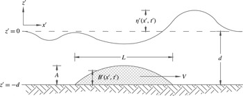
The 1DH landslide-wave problem in constant depth is sketched in figure 1. The landslide has a characteristic length
 $L$
, characteristic height
 $A$
, and travels at a constant speed
 $V$
in constant water depth
 $d$
. Here,
 $\unicode[STIX]{x1D702}^{\prime }(x^{\prime },t^{\prime })$
is the dimensional water surface elevation from the still water level and
 $B^{\prime }(x^{\prime },t^{\prime })$
denotes the bottom boundary deformation due to a landslide. As shown in Mei (Reference Mei1989), the solution to this type of problem, based on the linear and fully dispersive wave model (LFD), can be obtained by the use of Fourier and Laplace transforms. The dimensionless governing equation and the boundary conditions in constant water depth read
 $$\begin{eqnarray}\displaystyle \left.\begin{array}{@{}c@{}}\displaystyle \unicode[STIX]{x1D707}^{2}\unicode[STIX]{x1D719}_{xx}+\unicode[STIX]{x1D719}_{zz}=0,\quad -1<z<0,\\ \displaystyle \unicode[STIX]{x1D719}_{z}=\unicode[STIX]{x1D707}^{2}B_{t},\quad z=-1,\\ \displaystyle \unicode[STIX]{x1D719}_{z}=\unicode[STIX]{x1D707}^{2}\unicode[STIX]{x1D702}_{t},\quad z=0,\\ \displaystyle \unicode[STIX]{x1D719}_{t}+\unicode[STIX]{x1D702}=0,\quad z=0,\end{array}\right\} & & \displaystyle\end{eqnarray}$$
where
 $\unicode[STIX]{x1D719}=\unicode[STIX]{x1D719}(x,z,t)$
is the normalised velocity potential. The characteristic landslide height
 $A$
is assumed to be the same as the characteristic wave amplitude, and to linearise the problem,
 $A$
is required to be small compared with the water depth
 $d$
so that
 $O(A/d)=O(\unicode[STIX]{x1D716})\ll 1$
. The term
 $\unicode[STIX]{x1D707}=d/L$
controls how strong frequency dispersion is in the problem. The variables are normalised as
 $x=x^{\prime }/L$
,
 $z=z^{\prime }/d$
,
 $t=t^{\prime }\sqrt{gd}/L$
(
 $g$
is the gravitational acceleration),
 $\unicode[STIX]{x1D702}(x,t)=\unicode[STIX]{x1D702}^{\prime }(x^{\prime },t^{\prime })/A$
,
 $B(x,t)=B^{\prime }(x^{\prime },t^{\prime })/A$
and
 $\unicode[STIX]{x1D719}(x,z,t)=\unicode[STIX]{x1D719}^{\prime }(x^{\prime },z^{\prime },t^{\prime })/(\unicode[STIX]{x1D716}L\sqrt{gd})$
. The normalised landslide speed is defined as the Froude number:
 $Fr=V/\sqrt{gd}$
. After Laplace–Fourier-transforming (2.1), combining the equations, and imposing the initial conditions
 $$\begin{eqnarray}\displaystyle \unicode[STIX]{x1D702}(x,0)=0\quad \text{and}\quad \unicode[STIX]{x1D719}(x,0,0)=\text{const.}, & & \displaystyle\end{eqnarray}$$
where the second condition corresponds to zero initial horizontal velocity on the free surface, the transformed solution of
 $\unicode[STIX]{x1D702}(x,t)$
can be found as
 $$\begin{eqnarray}\displaystyle \overline{\widetilde{\unicode[STIX]{x1D702}}}(k,s)=\frac{\unicode[STIX]{x1D707}^{2}}{\cosh \unicode[STIX]{x1D707}k}\frac{s^{2}\overline{\widetilde{B}}-s\overline{B}(k,0)}{\unicode[STIX]{x1D707}^{2}s^{2}+\unicode[STIX]{x1D707}k\tanh \unicode[STIX]{x1D707}k}, & & \displaystyle\end{eqnarray}$$
which is the solution obtained in Mei (Reference Mei1989) for water waves forced by a general seafloor displacement
 $B(x,t)$
. While the definition of the Laplace transform is universal, that of the Fourier transform varies. In this study, the Fourier transform of a function
 $f(x)$
is defined as
 $$\begin{eqnarray}\displaystyle \left.\begin{array}{@{}c@{}}\displaystyle {\mathcal{F}}[f(x)](k)=\overline{f}(k)=\frac{1}{\sqrt{2\unicode[STIX]{x03C0}}}\int _{-\infty }^{\infty }f(x)\text{e}^{-\text{i}kx}\,\text{d}x,\\ \displaystyle {\mathcal{F}}^{-1}[\overline{f}(k)](x)=f(x)=\frac{1}{\sqrt{2\unicode[STIX]{x03C0}}}\int _{-\infty }^{\infty }\overline{f}(k)\text{e}^{\text{i}kx}\,\text{d}k.\end{array}\right\} & & \displaystyle\end{eqnarray}$$
While the overline is used to denote Fourier-transformed variables, the wide tilde is used to denote Laplace-transformed variables.
Definition sketch of the 1DH landslide-wave problem in constant depth.

For a translating landslide
 $B(x,t)=B(x-Fr\,t)=B(\unicode[STIX]{x1D709})$
, the Fourier transform can be written as
 $$\begin{eqnarray}\displaystyle \overline{B}(k,t) & = & \displaystyle \frac{1}{\sqrt{2\unicode[STIX]{x03C0}}}\int _{-\infty }^{\infty }B(x-Fr\,t)\text{e}^{-\text{i}kx}\,\text{d}x=\frac{1}{\sqrt{2\unicode[STIX]{x03C0}}}\int _{-\infty }^{\infty }B(\unicode[STIX]{x1D709})\text{e}^{-\text{i}kFr\,t}\text{e}^{-\text{i}k\unicode[STIX]{x1D709}}\,\text{d}\unicode[STIX]{x1D709}\nonumber\\ \displaystyle & = & \displaystyle \frac{1}{\sqrt{2\unicode[STIX]{x03C0}}}\text{e}^{-\text{i}kFr\,t}\int _{-\infty }^{\infty }B(x)\text{e}^{-\text{i}kx}\,\text{d}x=\overline{B(x,0)}\text{e}^{-\text{i}kFr\,t}.\end{eqnarray}$$
If such a landslide forcing function is used, a closed-form inverse Laplace transform is available, and the transformed solution (2.3) can be written as
 $$\begin{eqnarray}\displaystyle \left.\begin{array}{@{}c@{}}\displaystyle \unicode[STIX]{x1D702}(x,t)=\unicode[STIX]{x1D702}_{_{Fr}}(x,t)+\unicode[STIX]{x1D702}_{+}(x,t)+\unicode[STIX]{x1D702}_{-}(x,t),\\ \displaystyle \unicode[STIX]{x1D702}_{_{Fr}}(x,t)=-\frac{1}{\sqrt{2\unicode[STIX]{x03C0}}}\int _{-\infty }^{\infty }\frac{1}{\cosh \unicode[STIX]{x1D707}k}\frac{Fr^{2}}{D^{2}-Fr^{2}}\overline{B(x,0)}\text{e}^{-\text{i}kFr\,t}\text{e}^{\text{i}kx}\,\text{d}k,\\ \displaystyle \unicode[STIX]{x1D702}_{+}(x,t)=\frac{1}{\sqrt{2\unicode[STIX]{x03C0}}}\int _{-\infty }^{\infty }\frac{1}{\cosh \unicode[STIX]{x1D707}k}\frac{Fr}{2(D-Fr)}\overline{B(x,0)}\text{e}^{-\text{i}kDt}\text{e}^{\text{i}kx}\,\text{d}k,\\ \displaystyle \unicode[STIX]{x1D702}_{-}(x,t)=-\frac{1}{\sqrt{2\unicode[STIX]{x03C0}}}\int _{-\infty }^{\infty }\frac{1}{\cosh \unicode[STIX]{x1D707}k}\frac{Fr}{2(D+Fr)}\overline{B(x,0)}\text{e}^{\text{i}kDt}\text{e}^{\text{i}kx}\,\text{d}k,\end{array}\right\} & & \displaystyle\end{eqnarray}$$
where
 $$\begin{eqnarray}\displaystyle D=\sqrt{\frac{\tanh \unicode[STIX]{x1D707}k}{\unicode[STIX]{x1D707}k}} & & \displaystyle\end{eqnarray}$$
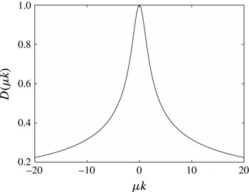
is the normalised wave speed in the LFD and is plotted in figure 2 as a function of
 $\unicode[STIX]{x1D707}k$
. It should be noted that
 $D(\unicode[STIX]{x1D707}k)$
has a maximum of one at
 $\unicode[STIX]{x1D707}k=0$
– the longest wave corresponding to
 $k=0$
travels at the fastest speed of one, and decays to zero as
 $|\unicode[STIX]{x1D707}k|$
increases – shorter waves (larger wavenumber
 $|k|$
) travel slower. Similarly to the analytical solution of the LSWEs, the three-wave structure is evident, but with additional frequency-dispersive effects – i.e. the wave speed
 $D$
depends on
 $k$
, allowing waves of different frequencies (wavenumbers) to travel at different speeds.
The frequency-dispersive wave speed
 $D(\unicode[STIX]{x1D707}k)$
(2.7) plotted as a function of
 $\unicode[STIX]{x1D707}k$
.

Since the solution for
 $\unicode[STIX]{x1D719}(x,z,t)$
is available and the horizontal and vertical velocities are given by
 $u(x,z,t)=\unicode[STIX]{x1D719}_{x}(x,z,t)$
and
 $w(x,z,t)=\unicode[STIX]{x1D719}_{z}(x,z,t)$
respectively, we can express the velocity solutions as
 $$\begin{eqnarray}\displaystyle \left.\begin{array}{@{}c@{}}\displaystyle u(x,z,t)=u_{_{Fr}}(x,z,t)+u_{+}(x,z,t)+u_{-}(x,z,t),\\ \displaystyle \!\!u_{_{Fr}}=-\frac{1}{\sqrt{2\unicode[STIX]{x03C0}}}\int _{-\infty }^{\infty }\frac{\overline{B(x,0)}}{\cosh \unicode[STIX]{x1D707}k}\frac{Fr^{2}}{D^{2}-Fr^{2}}\left(\frac{1}{Fr}\cosh (\unicode[STIX]{x1D707}kz)+\unicode[STIX]{x1D707}kFr\sinh (\unicode[STIX]{x1D707}kz)\right)\text{e}^{-\text{i}kFr\,t}\text{e}^{\text{i}kx}\,\text{d}k,\\ \displaystyle u_{+}=\frac{1}{\sqrt{2\unicode[STIX]{x03C0}}}\int _{-\infty }^{\infty }\frac{\overline{B(x,0)}}{\cosh \unicode[STIX]{x1D707}k}\frac{Fr}{2(D-Fr)}\left(\frac{1}{D}\cosh (\unicode[STIX]{x1D707}kz)+\unicode[STIX]{x1D707}kD\sinh (\unicode[STIX]{x1D707}kz)\right)\text{e}^{-\text{i}kDt}\text{e}^{\text{i}kx}\,\text{d}k,\\ \displaystyle u_{-}=\frac{1}{\sqrt{2\unicode[STIX]{x03C0}}}\int _{-\infty }^{\infty }\frac{\overline{B(x,0)}}{\cosh \unicode[STIX]{x1D707}k}\frac{Fr}{2(D+Fr)}\left(\frac{1}{D}\cosh (\unicode[STIX]{x1D707}kz)+\unicode[STIX]{x1D707}kD\sinh (\unicode[STIX]{x1D707}kz)\right)\text{e}^{\text{i}kDt}\text{e}^{\text{i}kx}\,\text{d}k\end{array}\right\} & & \displaystyle \nonumber\\ \displaystyle & & \displaystyle\end{eqnarray}$$
and
 $$\begin{eqnarray}\displaystyle \left.\begin{array}{@{}c@{}}\displaystyle w(x,z,t)=w_{_{Fr}}(x,z,t)+w_{+}(x,z,t)+w_{-}(x,z,t),\\ \displaystyle w_{_{Fr}}=\frac{\text{i}\unicode[STIX]{x1D707}}{\sqrt{2\unicode[STIX]{x03C0}}}\int _{-\infty }^{\infty }\frac{\overline{B(x,0)}}{\cosh \unicode[STIX]{x1D707}k}\frac{Fr^{2}}{D^{2}-Fr^{2}}\left(\frac{1}{Fr}\sinh (\unicode[STIX]{x1D707}kz)+\unicode[STIX]{x1D707}kFr\cosh (\unicode[STIX]{x1D707}kz)\right)\text{e}^{-\text{i}kFr\,t}\text{e}^{\text{i}kx}\,\text{d}k,\\ \displaystyle w_{+}=-\frac{\text{i}\unicode[STIX]{x1D707}}{\sqrt{2\unicode[STIX]{x03C0}}}\int _{-\infty }^{\infty }\frac{\overline{B(x,0)}}{\cosh \unicode[STIX]{x1D707}k}\frac{Fr}{2(D-Fr)}\left(\frac{1}{D}\sinh (\unicode[STIX]{x1D707}kz)+\unicode[STIX]{x1D707}kD\cosh (\unicode[STIX]{x1D707}kz)\right)\text{e}^{-\text{i}kDt}\text{e}^{\text{i}kx}\,\text{d}k,\\ \displaystyle w_{-}=-\frac{\text{i}\unicode[STIX]{x1D707}}{\sqrt{2\unicode[STIX]{x03C0}}}\int _{-\infty }^{\infty }\frac{\overline{B(x,0)}}{\cosh \unicode[STIX]{x1D707}k}\frac{Fr}{2(D+Fr)}\left(\frac{1}{D}\sinh (\unicode[STIX]{x1D707}kz)+\unicode[STIX]{x1D707}kD\cosh (\unicode[STIX]{x1D707}kz)\right)\text{e}^{\text{i}kDt}\text{e}^{\text{i}kx}\,\text{d}k.\end{array}\right\} & & \displaystyle \nonumber\\ \displaystyle & & \displaystyle\end{eqnarray}$$
Unlike the LSWEs, in the LFD, the free-surface elevation and the velocity potential (and thus the velocities) cannot be solved separately. The imposed initial conditions
 $\unicode[STIX]{x1D702}(x,0)=0$
and
 $\unicode[STIX]{x1D719}(x,0,0)=\text{const.}$
are therefore enforced in all solutions. It should be noted that, due to allowance of flow variation in the vertical (
 $z$
) direction, the initial flow velocity cannot be everywhere zero in the LFD for a landslide moving at a constant speed.
2.1.2 Far-field leading-wave solution
For
 $Fr\neq 1$
and given sufficient propagation time, the three waves in the solution (2.6) –
 $\unicode[STIX]{x1D702}_{_{Fr}}$
,
 $\unicode[STIX]{x1D702}_{+}$
and
 $\unicode[STIX]{x1D702}_{-}$
– eventually separate from each other. Here,
 $\unicode[STIX]{x1D702}_{+}$
and
 $\unicode[STIX]{x1D702}_{-}$
are the free waves that travel in opposite directions, and their shapes evolve in time due to frequency dispersion, whereas
 $\unicode[STIX]{x1D702}_{_{Fr}}$
is the trapped wave that moves with the landslide and has a permanent shape, as can be seen by the
 $\text{e}^{\text{i}k(x-Fr\,t)}$
term in the solution (2.6). The method of stationary phase (for more details, see Mei Reference Mei1989; Bender & Orszag Reference Bender and Orszag1999) can be used on frequency-dispersive free-wave solutions like
 $\unicode[STIX]{x1D702}_{+}$
and
 $\unicode[STIX]{x1D702}_{-}$
to obtain closed-form asymptotic far-field leading-wave solutions valid for large
 $t$
and near
 $x=t$
. Resonance occurs for
 $Fr=1$
and will be discussed in the next section.
Since the approximation process to obtain the far-field leading-wave solution (accurate for large
 $t$
and near
 $x=t$
) is fairly standard and has been described in Mei (Reference Mei1989), here, we skip the derivation and simply present the result – keeping the first three (leading-order, second-order and third-order) terms in the approximation, we obtain the far-field leading-wave solution
 $\unicode[STIX]{x1D702}_{+}^{\ast }(x,t)$
for the right-going wave:
 $$\begin{eqnarray}\displaystyle \unicode[STIX]{x1D702}_{+}^{\ast }(x,t) & = & \displaystyle S\frac{Fr}{2(1-Fr)}\left(\frac{2}{\unicode[STIX]{x1D707}^{2}t}\right)^{1/3}\text{Ai}\left[\left(\frac{2}{\unicode[STIX]{x1D707}^{2}t}\right)^{1/3}(x-t)\right]\nonumber\\ \displaystyle & & \displaystyle -\,M_{1}\frac{Fr}{2(1-Fr)}\left(\frac{2}{\unicode[STIX]{x1D707}^{2}t}\right)^{2/3}\text{Ai}^{\prime }\left[\left(\frac{2}{\unicode[STIX]{x1D707}^{2}t}\right)^{1/3}(x-t)\right]\nonumber\\ \displaystyle & & \displaystyle +\,\frac{M_{2}}{2}\frac{Fr}{2(1-Fr)}\left(\frac{2}{\unicode[STIX]{x1D707}^{2}t}\right)\text{Ai}^{\prime \prime }\left[\left(\frac{2}{\unicode[STIX]{x1D707}^{2}t}\right)^{1/3}(x-t)\right]+\cdots \,,\end{eqnarray}$$
where
 $\text{Ai}$
is the Airy function,
 $S$
is the area enclosed by the landslide,
 $M_{1}$
is the first moment of the landslide forcing function at
 $t=0$
(i.e.
 $M_{1}=\int _{-\infty }^{\infty }xB(x)\,\text{d}x$
) and
 $M_{2}$
is the second moment (i.e.
 $M_{2}=\int _{-\infty }^{\infty }x^{2}B(x)\,\text{d}x$
). For a physical landslide,
 $S>0$
and the first moment can be written as
 $M_{1}=Sx_{c}$
, where
 $x_{c}$
is the initial centre of mass of the landslide forcing function at
 $t=0$
. Hence, the first two terms of the far-field leading-wave solution (2.10) depend only on the area enclosed by the landslide, and the effect of the exact landslide shape first appears in the third-order term, in the form of the second moment
 $M_{2}$
. It should be noted that, since (2.10) is accurate only near
 $x=t$
, it is preferable to define the coordinate system such that
 $x_{c}=0$
to ensure that the leading wave indeed travels along
 $x\simeq t$
. If
 $x_{c}\neq 0$
is chosen, the asymptotic solution (2.10) still holds, but would require a longer time
 $t$
for the asymptotic solution to become accurate.
A similar procedure can be performed on the left-going wave
 $\unicode[STIX]{x1D702}_{-}$
to obtain the far-field leading-wave solution
 $\unicode[STIX]{x1D702}_{-}^{\ast }(x,t)$
:
 $$\begin{eqnarray}\displaystyle \unicode[STIX]{x1D702}_{-}^{\ast }(x,t) & = & \displaystyle -S\frac{Fr}{2(1+Fr)}\left(\frac{2}{\unicode[STIX]{x1D707}^{2}t}\right)^{1/3}\text{Ai}\left[-\!\left(\frac{2}{\unicode[STIX]{x1D707}^{2}t}\right)^{1/3}(x+t)\right]\nonumber\\ \displaystyle & & \displaystyle +\,M_{1}\frac{Fr}{2(1+Fr)}\left(\frac{2}{\unicode[STIX]{x1D707}^{2}t}\right)^{2/3}\text{Ai}^{\prime }\left[-\!\left(\frac{2}{\unicode[STIX]{x1D707}^{2}t}\right)^{1/3}(x+t)\right]\nonumber\\ \displaystyle & & \displaystyle -\,\frac{M_{2}}{2}\frac{Fr}{2(1+Fr)}\left(\frac{2}{\unicode[STIX]{x1D707}^{2}t}\right)\text{Ai}^{\prime \prime }\left[-\!\left(\frac{2}{\unicode[STIX]{x1D707}^{2}t}\right)^{1/3}(x+t)\right]+\cdots \,,\end{eqnarray}$$
which is accurate for large
 $t$
and near
 $x=-t$
. It should be noted that (2.11) and (2.10) are similar, except for the sign difference and that the amplitude of (2.11) is much smaller in the vicinity of
 $Fr\sim 1$
– i.e. resonance does not occur for the left-going wave. In addition, we remark that the far-field leading-wave solutions due to a translating landslide are similar to those due to an impulsive seafloor displacement derived in Mei (Reference Mei1989), the main difference being the additional
 $Fr$
(landslide speed) effects on the wave amplitudes.
While the far-field leading-wave solution becomes a better and better approximation near
 $x=t$
as
 $t\rightarrow \infty$
, the accuracy of all solutions is limited by the accuracy of the governing equation, i.e. the truncation error
 $O(\unicode[STIX]{x1D716})$
of the LFD. In reality, as
 $t\rightarrow \infty$
, the nonlinearity in an initially linear problem eventually grows sufficiently that
 $O(\unicode[STIX]{x1D716})$
becomes significant, and the linear far-field solution breaks down when
 $t\gg O(1/\unicode[STIX]{x1D716})$
.
2.1.3 Landslide shape effect on the far-field leading wave
The far-field leading-wave solutions (2.10) and (2.11) indicate that the area
 $S$
enclosed by the landslide has the most important effect on the leading wave, and that the exact landslide shape first becomes relevant in the third-order term, which decays faster at the rate
 $t^{-1}$
than the leading-order terms. As
 $t$
becomes large, eventually the leading wave is affected by only the leading-order terms that depend on
 $S$
. This analytical finding therefore supports the belief that it is more important to match the landslide area (or volume) in modelling than the exact landslide shape.
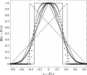
To check the performance of the far-field leading-wave solutions, we use (2.10) as an example and consider seven different landslide shapes that have the same characteristic height and area enclosed, initially centred at the origin so that
 $x_{c}=0=M_{1}$
: a Gaussian curve (
 $B_{1}$
), a parabolic cap (
 $B_{2}$
), a quartic cap (
 $B_{3}$
), a rectangle (
 $B_{4}$
) and three different triangles (
 $B_{5}$
,
 $B_{6}$
and
 $B_{7}$
). The seven different landslide shapes are compared in figure 3, and the mathematical details on the shape definitions and their Fourier transforms are provided in appendix A. These analytical expressions are then used in (2.6) to obtain the exact solutions.
Comparison of the seven different landslide shapes that all have the same height, enclosed area and centre of mass
 $x_{c}=0$
: circle, Gaussian curve (
 $B_{1}$
); cross, parabolic cap (
 $B_{2}$
); plus, quartic cap (
 $B_{3}$
); dotted line, rectangle (
 $B_{4}$
); solid line, triangle (
 $B_{5}$
); dashed line, triangle (
 $B_{6}$
); dash–dot line, triangle (
 $B_{7}$
).

Since these landslides all have the same height, enclosed area and centre of mass
 $x_{c}=0$
, we expect the exact analytical solutions to all eventually converge to the same asymptotic leading-wave solution (near
 $x=t$
) as
 $t$
increases. For
 $\unicode[STIX]{x1D707}=0.25$
and
 $Fr=0.5$
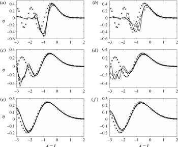
, in figure 4 we compare the far-field leading-wave solution (2.10), with only the first-order term (note that the second-order term is zero since
 $x_{c}=0$
), with the numerically integrated complete solution (2.6) for the seven different landslide shapes at three different times
 $t=2,5,10$
. We see that although the initial wave fields due to different landslide shapes can be very different, as time increases, the leading waves indeed all converge to the same leading-order asymptotic solution, which depends on the area enclosed by the landslide.
Comparison of water waves generated by landslides of different shapes with initial centres of mass
 $x_{c}=0$
, for
 $\unicode[STIX]{x1D707}=0.25$
and
 $Fr=0.5$
: (a,b)
 $t=2$
; (c,d)
 $t=5$
; (e,f)
 $t=10$
. (a,c,e) Solid line, Gaussian curve (
 $B_{1}$
); dotted line, parabolic cap (
 $B_{2}$
); dashed line, quartic cap (
 $B_{3}$
); dash–dot line, rectangle (
 $B_{4}$
); cross, equation (2.10) with only the leading-order term. (b,d,f) Solid line, triangle (
 $B_{5}$
); dotted line, triangle (
 $B_{6}$
); dashed line, triangle
 $B_{7}$
; cross, asymptotic solution (2.10) with only the leading-order term.

2.1.4 Resonance solution
In the complete 1DH LFD solutions (2.6), we observe that discontinuities exist for
 $0<D(\unicode[STIX]{x1D707}k)=Fr\leqslant 1$
(recall that as plotted in figure 2,
 $D(\unicode[STIX]{x1D707}k)$
has a maximum of one at
 $\unicode[STIX]{x1D707}k=0$
), when resonance appears to occur. Although the modal resonance solution (for when
 $D(\unicode[STIX]{x1D707}k)=Fr$
) similar to (1.5) can be obtained, it is not very meaningful since an integration over the wavenumber (
 $k$
) space is necessary to obtain the full LFD solution, and the contribution due to single modes is lost due to the integration. For the LFD, it is therefore more meaningful to examine how the solution behaves near the discontinuities, as opposed to at the discontinuities. In appendix B, we show that only the
 $Fr=1$
resonance mode is significant, in which the right-going wave may grow indefinitely in time. We will thus focus only on the
 $Fr=1$
resonance mode.
In the complete LFD solution (2.6),
 $\unicode[STIX]{x1D702}_{_{Fr}}$
is the steady-state component, which is of a permanent form and moves at the same speed as the landslide, as indicated by the
 $\text{e}^{\text{i}k(x-Fr\,t)}$
term. The terms
 $\unicode[STIX]{x1D702}_{+}$
and
 $\unicode[STIX]{x1D702}_{-}$
are the transient components that evolve in time due to frequency dispersion, as indicated by the
 $\text{e}^{\text{i}k(x-Dt)}$
and
 $\text{e}^{\text{i}k(x+Dt)}$
terms. When resonance occurs (
 $Fr=1$
),
 $\unicode[STIX]{x1D702}_{_{Fr}}$
and
 $\unicode[STIX]{x1D702}_{+}$
become inseparable and together form the leading wave. Since
 $\unicode[STIX]{x1D702}_{_{Fr}}$
is of a permanent form, the growth rate of the leading wave is solely determined by that of
 $\unicode[STIX]{x1D702}_{+}$
. For
 $Fr=1$
, the leading-order far-field leading-wave approximation (valid for large
 $t$
and near
 $x=t$
) for
 $\unicode[STIX]{x1D702}_{+}$
can be found by using the method of stationary phase to be
 $$\begin{eqnarray}\displaystyle \unicode[STIX]{x1D702}_{+}^{\ast }(x,t) & = & \displaystyle \frac{1}{2\unicode[STIX]{x03C0}}S\int _{-\infty }^{\infty }\frac{-3}{\unicode[STIX]{x1D707}^{2}k^{2}}\text{e}^{\text{i}[kx-kt+(1/6)k^{3}\unicode[STIX]{x1D707}^{2}t]}\,\text{d}k+\cdots \nonumber\\ \displaystyle & = & \displaystyle \frac{-3}{2\unicode[STIX]{x03C0}\unicode[STIX]{x1D707}^{2}}\left(\frac{\unicode[STIX]{x1D707}^{2}t}{2}\right)^{1/3}S\int _{-\infty }^{\infty }\frac{1}{q^{2}}\text{e}^{\text{i}[(2/\unicode[STIX]{x1D707}^{2}t)^{1/3}(x-t)q+(1/3)q^{3}]}\,\text{d}q+\cdots \,,\end{eqnarray}$$
where the substitution
 $k=(2/\unicode[STIX]{x1D707}^{2}t)^{1/3}q$
is used to rewrite the
 $k$
-integral and
 $S$
is again the area enclosed by the landslide. It should be noted that the
 $q$
-integral is solely a function of
 $(2/\unicode[STIX]{x1D707}^{2}t)^{1/3}(x-t)$
, defined similarly to the Airy function but with the addition of
 $1/q^{2}$
in the integrand. Since the shape of the far-field leading wave is determined by the
 $q$
-integral, we see that the resonance far-field leading-wave solution grows in time at the rate
 $t^{1/3}$
, instead of decaying at the rate
 $t^{-1/3}$
, which is the case for
 $Fr\neq 1$
.
Although the far-field leading-wave approximation for
 $\unicode[STIX]{x1D702}_{+}$
, equation (2.12), can be obtained and the growth rate examined, it should be noted that the improper integral in (2.12) is infinite due to the factor
 $1/q^{2}$
. In fact, the far-field leading-wave solution consists of both (2.12) and
 $\unicode[STIX]{x1D702}_{_{Fr}}$
, which is of a permanent form and also has an infinite magnitude for
 $Fr=1$
. Taylor series expansions about the discontinuities can be used to show that the two infinite magnitudes cancel out and the results end up finite. The complete far-field leading-wave solution (valid for large
 $t$
and near
 $x=t$
) is therefore
 $$\begin{eqnarray}\displaystyle \unicode[STIX]{x1D702}_{lead}(x,t)=\unicode[STIX]{x1D702}_{_{Fr}}(x,t)+\unicode[STIX]{x1D702}_{+}^{\ast }(x,t),\quad Fr=1. & & \displaystyle\end{eqnarray}$$
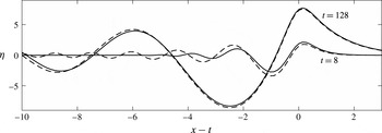
Equation (2.13) and the complete solution (2.6) are compared in figure 5, for a Gaussian landslide forcing function moving at a constant speed
 $Fr=1$
:
 $B(x,t)=\text{e}^{-8(x-t)^{2}}$
with
 $\unicode[STIX]{x1D707}=0.3$
. We see that the far-field leading-wave solution (2.13) indeed becomes more accurate near
 $x=t$
as
 $t$
increases. Nonetheless, we remark that for the resonance case the most important information gained from the far-field leading-wave solution is the growth rate
 $t^{1/3}$
, as indicated by (2.12). The asymptotic wave profile (2.13) is of little practical value since a numerical integration is still needed for plotting – computing the asymptotic solution (2.13) presents few benefits over computing the complete solution (2.6).


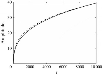
To test the asymptotic growth rate
 $t^{1/3}$
, we numerically compute the full LFD solution (2.6) for a Gaussian landslide forcing function moving at a constant speed
 $Fr=1$
with
 $\unicode[STIX]{x1D707}=0.3$
. The actual growth rate of the leading wave, obtained by determining the maximum height in space of the wave crest near
 $x=t$
in the full LFD solution (2.6), is then compared with the asymptotic rate of
 $t^{1/3}$
in figure 6. We see that the leading-wave-amplitude growth rate indeed approaches
 $t^{1/3}$
as
 $t$
increases.
Amplitude of the leading wave as a function of
 $t$
, for a Gaussian landslide forcing function with
 $Fr=1$
and
 $\unicode[STIX]{x1D707}=0.3$
: solid line, the complete LFD solution (2.6); dashed line, the asymptotic growth rate
 $t^{1/3}$
.

2.2 One-dimensional (horizontal) linear and weakly dispersive model
The linear and weakly dispersive model (LWD) can be obtained by linearising the Boussinesq equations (Nwogu Reference Nwogu1993) or the fully nonlinear and weakly dispersive model (Wei et al.
Reference Wei, Kirby, Grilli and Subramanya1995; Lynett & Liu Reference Lynett and Liu2002). Alternatively, it can be obtained as an approximated version of the LFD based on the long-wave assumption (see, for example, Lynett & Liu (Reference Lynett and Liu2002), who demonstrated how to obtain weakly dispersive models from a fully dispersive model). The LWD is accurate when both
 $O(\unicode[STIX]{x1D716})\ll 1$
and
 $O(\unicode[STIX]{x1D707}^{4})\ll 1$
. In weakly dispersive models, the governing equations are often solved at a representative depth
 $z_{\unicode[STIX]{x1D6FC}}$
, which is chosen to improve the characteristics of frequency dispersion; the horizontal velocity at depth
 $z=z_{\unicode[STIX]{x1D6FC}}$
is written as
 $u(x,z_{\unicode[STIX]{x1D6FC}},t)=u_{\unicode[STIX]{x1D6FC}}(x,t)$
. For the LWD in constant depth,
 $z_{\unicode[STIX]{x1D6FC}}=\unicode[STIX]{x1D6FC}$
since the normalised water depth is
 $1$
, and here we use
 $\unicode[STIX]{x1D6FC}=-0.531$
as recommended by Nwogu (Reference Nwogu1993). The dimensionless continuity equation reads
 $$\begin{eqnarray}\displaystyle \unicode[STIX]{x1D702}_{t}+u_{\unicode[STIX]{x1D6FC}x}+\unicode[STIX]{x1D6FC}_{11}u_{\unicode[STIX]{x1D6FC}xxx}=B_{t}+\unicode[STIX]{x1D6FC}_{12}B_{txx} & & \displaystyle\end{eqnarray}$$
and the momentum equation reads
 $$\begin{eqnarray}\displaystyle u_{\unicode[STIX]{x1D6FC}t}+\unicode[STIX]{x1D6FC}_{21}u_{\unicode[STIX]{x1D6FC}xxt}+\unicode[STIX]{x1D702}_{x}=\unicode[STIX]{x1D6FC}_{22}B_{txt}, & & \displaystyle\end{eqnarray}$$
where
 $\unicode[STIX]{x1D6FC}_{11}$
,
 $\unicode[STIX]{x1D6FC}_{12}$
,
 $\unicode[STIX]{x1D6FC}_{21}$
and
 $\unicode[STIX]{x1D6FC}_{22}$
are constants:
 $$\begin{eqnarray}\displaystyle \left.\begin{array}{@{}c@{}}\displaystyle \unicode[STIX]{x1D6FC}_{11}=\unicode[STIX]{x1D707}^{2}\left({\textstyle \frac{1}{2}}\unicode[STIX]{x1D6FC}^{2}+\unicode[STIX]{x1D6FC}+{\textstyle \frac{1}{3}}\right),\quad \unicode[STIX]{x1D6FC}_{12}=\unicode[STIX]{x1D707}^{2}\left(\unicode[STIX]{x1D6FC}+{\textstyle \frac{1}{2}}\right),\quad \unicode[STIX]{x1D6FC}_{21}=\unicode[STIX]{x1D707}^{2}\left({\textstyle \frac{1}{2}}\unicode[STIX]{x1D6FC}^{2}+\unicode[STIX]{x1D6FC}\right),\quad \unicode[STIX]{x1D6FC}_{22}=\unicode[STIX]{x1D707}^{2}\unicode[STIX]{x1D6FC},\\ \displaystyle \unicode[STIX]{x1D6FC}=-0.531.\end{array}\right\} & & \displaystyle \nonumber\\ \displaystyle & & \displaystyle\end{eqnarray}$$
Solving for
 $u_{\unicode[STIX]{x1D6FC}}$
first is more convenient in this case, and (2.14) and (2.15) can be combined to yield
 $$\begin{eqnarray}\displaystyle u_{\unicode[STIX]{x1D6FC}xx}-u_{\unicode[STIX]{x1D6FC}tt}+\unicode[STIX]{x1D6FC}_{11}u_{\unicode[STIX]{x1D6FC}xxxx}-\unicode[STIX]{x1D6FC}_{21}u_{\unicode[STIX]{x1D6FC}xxtt}=B_{tx}+\unicode[STIX]{x1D6FC}_{12}B_{txxx}-\unicode[STIX]{x1D6FC}_{22}B_{ttxt}. & & \displaystyle\end{eqnarray}$$
The LWD can be solved in a manner similar to those for the LSWEs and the LFD and here we only outline the solution process. When
 $u_{\unicode[STIX]{x1D6FC}}$
is solved for first, the imposed initial conditions are
 $$\begin{eqnarray}\displaystyle u_{\unicode[STIX]{x1D6FC}}(x,0)=\unicode[STIX]{x1D707}^{2}z_{\unicode[STIX]{x1D6FC}}B_{tx}\quad \text{and}\quad u_{\unicode[STIX]{x1D6FC}t}(x,0)+\unicode[STIX]{x1D6FC}_{21}u_{\unicode[STIX]{x1D6FC}xxt}(x,0)=\unicode[STIX]{x1D6FC}_{22}B_{xtt}(x,0). & & \displaystyle\end{eqnarray}$$
The first condition results from setting
 $u(x,0,0)=0$
(initial horizontal velocity on the free surface is zero) and recovering
 $u_{\unicode[STIX]{x1D6FC}}(x,0)$
from the velocity profile assumed in the LWD. The second condition results from setting
 $\unicode[STIX]{x1D702}_{x}(x,0)=0$
in (2.15); thus,
 $\unicode[STIX]{x1D702}(x,0)=\text{const}$
. If the derivatives of
 $u_{\unicode[STIX]{x1D6FC}}$
and
 $B$
are all continuous, the order of differentiation does not matter. By Laplace–Fourier-transforming (2.17) and applying the above initial conditions, equation (2.17) becomes
 $$\begin{eqnarray}\displaystyle -\!k^{2}\overline{\widetilde{u_{\unicode[STIX]{x1D6FC}}}}-s^{2}\overline{\widetilde{u_{\unicode[STIX]{x1D6FC}}}}+\unicode[STIX]{x1D6FC}_{11}k^{4}\overline{\widetilde{u_{\unicode[STIX]{x1D6FC}}}}+\unicode[STIX]{x1D6FC}_{21}s^{2}k^{2}\overline{\widetilde{u_{\unicode[STIX]{x1D6FC}}}}=\text{i}k(1-\unicode[STIX]{x1D6FC}_{12}k^{2}-\unicode[STIX]{x1D6FC}_{22}s^{2})[s\overline{\widetilde{B}}-\overline{B}(k,0)], & & \displaystyle\end{eqnarray}$$
from which
 $\overline{\widetilde{u_{\unicode[STIX]{x1D6FC}}}}$
can be solved for as
 $$\begin{eqnarray}\displaystyle \overline{\widetilde{u_{\unicode[STIX]{x1D6FC}}}}(k,s)=\frac{\text{i}k(1-\unicode[STIX]{x1D6FC}_{12}k^{2}-\unicode[STIX]{x1D6FC}_{22}s^{2})[s\overline{\widetilde{B}}-\overline{B}(k,0)]}{(\unicode[STIX]{x1D6FC}_{11}k^{2}-1)k^{2}+(\unicode[STIX]{x1D6FC}_{21}k^{2}-1)s^{2}}. & & \displaystyle\end{eqnarray}$$
The
 $\overline{\widetilde{\unicode[STIX]{x1D702}}}$
can then be recovered from transformed (2.14) or (2.15). If (2.14) is used, we obtain
 $$\begin{eqnarray}\displaystyle \overline{\widetilde{\unicode[STIX]{x1D702}}}(k,s)=\frac{s\overline{\widetilde{B}}-\overline{B}(k,0)}{s}\left[(1-\unicode[STIX]{x1D6FC}_{12}k^{2})-\displaystyle \frac{k^{2}\displaystyle \frac{1-\unicode[STIX]{x1D6FC}_{11}k^{2}}{1-\unicode[STIX]{x1D6FC}_{21}k^{2}}(1-\unicode[STIX]{x1D6FC}_{12}k^{2}-\unicode[STIX]{x1D6FC}_{22}s^{2})}{s^{2}+k^{2}\displaystyle \frac{1-\unicode[STIX]{x1D6FC}_{11}k^{2}}{1-\unicode[STIX]{x1D6FC}_{21}k^{2}}}\right]+\frac{\overline{\unicode[STIX]{x1D702}(x,0)}}{s}. & & \displaystyle \nonumber\\ \displaystyle & & \displaystyle\end{eqnarray}$$
Since
 $u_{\unicode[STIX]{x1D6FC}}$
is solved for first in this case, the precise initial condition for the free surface,
 $\unicode[STIX]{x1D702}(x,0)$
, can be specified only when the solution for
 $\unicode[STIX]{x1D702}$
is considered. Here, we require
 $\unicode[STIX]{x1D702}(x,0)=0$
.
For a translating landslide moving at a constant speed
 $Fr$
so that
 $B(x,t)=B(x-Fr\,t)$
, a closed-form inverse Laplace transform of (2.21) is available, and we find
 $\unicode[STIX]{x1D702}(x,t)$
to be
 $$\begin{eqnarray}\displaystyle \left.\begin{array}{@{}c@{}}\displaystyle \unicode[STIX]{x1D702}(x,t)=\unicode[STIX]{x1D702}_{_{Fr}}(x,t)+\unicode[STIX]{x1D702}_{+}(x,t)+\unicode[STIX]{x1D702}_{-}(x,t),\\ \displaystyle \unicode[STIX]{x1D702}_{_{Fr}}(x,t)=-\frac{1}{\sqrt{2\unicode[STIX]{x03C0}}}\int _{-\infty }^{\infty }(1-\unicode[STIX]{x1D6FC}_{12}k^{2}+\unicode[STIX]{x1D6FC}_{22}k^{2}D^{2})\frac{Fr^{2}}{D^{2}-Fr^{2}}\overline{B(x,0)}\text{e}^{-\text{i}kFr\,t}\text{e}^{\text{i}kx}\,\text{d}k,\\ \displaystyle \unicode[STIX]{x1D702}_{+}(x,t)=\frac{1}{\sqrt{2\unicode[STIX]{x03C0}}}\int _{-\infty }^{\infty }(1-\unicode[STIX]{x1D6FC}_{12}k^{2}+\unicode[STIX]{x1D6FC}_{22}k^{2}D^{2})\frac{Fr}{2(D-Fr)}\overline{B(x,0)}\text{e}^{-\text{i}kDt}\text{e}^{\text{i}kx}\,\text{d}k,\\ \displaystyle \unicode[STIX]{x1D702}_{-}(x,t)=-\frac{1}{\sqrt{2\unicode[STIX]{x03C0}}}\int _{-\infty }^{\infty }(1-\unicode[STIX]{x1D6FC}_{12}k^{2}+\unicode[STIX]{x1D6FC}_{22}k^{2}D^{2})\frac{Fr}{2(D+Fr)}\overline{B(x,0)}\text{e}^{\text{i}kDt}\text{e}^{\text{i}kx}\,\text{d}k,\end{array}\right\} & & \displaystyle\end{eqnarray}$$
where
 $$\begin{eqnarray}\displaystyle D=\sqrt{\frac{1-\unicode[STIX]{x1D6FC}_{11}k^{2}}{1-\unicode[STIX]{x1D6FC}_{21}k^{2}}} & & \displaystyle\end{eqnarray}$$
is the normalised wave speed of the LWD. We again see the three-wave structure and frequency-dispersive effects. Equations (2.22) and (2.23) are highly similar to (2.6) and (2.7) as the LWD is essentially an expanded (approximated) version of the LFD (the verification is shown in appendix C), based on the long-wave assumption. The same asymptotic approximation method can be used to obtain the far-field leading-wave solutions of (2.22), and the results will be exactly the same as those for the LFD, since the leading-wave solution depends on only the leading-order
 $O(\unicode[STIX]{x1D707}^{2})$
frequency-dispersive effects which are included in the LWD. The leading wave in the resonance case (
 $Fr=1$
) therefore also grows at the rate
 $t^{1/3}$
.
Similarly, a closed-form inverse Laplace transform of (2.20) is available, and we can express
 $u_{\unicode[STIX]{x1D6FC}}$
, the horizontal velocity at depth
 $z_{\unicode[STIX]{x1D6FC}}$
, as
 $$\begin{eqnarray}\displaystyle \left.\begin{array}{@{}c@{}}\displaystyle u_{\unicode[STIX]{x1D6FC}}(x,t)=u_{\unicode[STIX]{x1D6FC}_{Fr}}(x,t)+u_{\unicode[STIX]{x1D6FC}_{+}}(x,t)+u_{\unicode[STIX]{x1D6FC}_{-}}(x,t),\\ \displaystyle u_{\unicode[STIX]{x1D6FC}_{Fr}}(x,t)=-\frac{1}{\sqrt{2\unicode[STIX]{x03C0}}}\int _{-\infty }^{\infty }\frac{\overline{B(x,0)}}{1-\unicode[STIX]{x1D6FC}_{21}k^{2}}\frac{Fr^{2}}{D^{2}-Fr^{2}}\frac{1-\unicode[STIX]{x1D6FC}_{12}k^{2}+\unicode[STIX]{x1D6FC}_{22}k^{2}Fr^{2}}{Fr}\text{e}^{-\text{i}kFr\,t}\text{e}^{\text{i}kx}\,\text{d}k,\\ \displaystyle u_{\unicode[STIX]{x1D6FC}_{+}}(x,t)=\frac{1}{\sqrt{2\unicode[STIX]{x03C0}}}\int _{-\infty }^{\infty }\frac{\overline{B(x,0)}}{1-\unicode[STIX]{x1D6FC}_{21}k^{2}}\frac{Fr}{2(D-Fr)}\frac{1-\unicode[STIX]{x1D6FC}_{12}k^{2}+\unicode[STIX]{x1D6FC}_{22}k^{2}D^{2}}{D}\text{e}^{-\text{i}kDt}\text{e}^{\text{i}kx}\,\text{d}k,\\ \displaystyle u_{\unicode[STIX]{x1D6FC}_{-}}(x,t)=\frac{1}{\sqrt{2\unicode[STIX]{x03C0}}}\int _{-\infty }^{\infty }\frac{\overline{B(x,0)}}{1-\unicode[STIX]{x1D6FC}_{21}k^{2}}\frac{Fr}{2(D+Fr)}\frac{1-\unicode[STIX]{x1D6FC}_{12}k^{2}+\unicode[STIX]{x1D6FC}_{22}k^{2}D^{2}}{D}\text{e}^{\text{i}kDt}\text{e}^{\text{i}kx}\,\text{d}k.\end{array}\right\}\qquad & & \displaystyle\end{eqnarray}$$
The full horizontal and vertical velocities (
 $u$
and
 $w$
respectively) in the LWD can be expressed as
 $$\begin{eqnarray}\displaystyle \left.\begin{array}{@{}c@{}}\displaystyle u(x,z,t)=u_{\unicode[STIX]{x1D6FC}}(x,t)-\unicode[STIX]{x1D707}^{2}\left({\textstyle \frac{1}{2}}(z^{2}-\unicode[STIX]{x1D6FC}^{2})u_{\unicode[STIX]{x1D6FC}xx}+(z-\unicode[STIX]{x1D6FC})(u_{\unicode[STIX]{x1D6FC}xx}-B_{tx})\right)+O(\unicode[STIX]{x1D707}^{4}),\\ \displaystyle w(x,z,t)=-\unicode[STIX]{x1D707}^{2}\left(zu_{x}(x,0,t)+u_{x}(x,0,t)-B_{t}\right)+O(\unicode[STIX]{x1D707}^{4}).\end{array}\right\} & & \displaystyle\end{eqnarray}$$
It should be noted that the expressions in (2.25) are not unique, since alternate
 $O(\unicode[STIX]{x1D707}^{2})$
terms may be used. For more details on recovering the velocity field from
 $u_{\unicode[STIX]{x1D6FC}}$
in weakly dispersive models, see, for example, Lynett & Liu (Reference Lynett and Liu2002).
2.3 Comparison of the analytical solutions
The analytical solutions based on different wave models (LSWE, LWD and LFD) are compared (integral-form solutions are numerically integrated when necessary) in this section for a selected example. Since LSWE has a theoretical truncation error of
 $O(\unicode[STIX]{x1D707}^{2})$
, LWD has a theoretical truncation error of
 $O(\unicode[STIX]{x1D707}^{4})$
and LFD has no restriction on
 $\unicode[STIX]{x1D707}$
, we expect the three models to yield essentially identical results for a very long landslide with small
 $\unicode[STIX]{x1D707}$
(recall that
 $\unicode[STIX]{x1D707}$
is water depth divided by landslide length). As the landslide length shortens, LSWE and LWD become less and less accurate.
We have found
 $\unicode[STIX]{x1D707}=0.2$
to be an intermediate landslide length for which LSWE is inaccurate but LWD remains accurate. For a Gaussian-shaped landslide with
 $\unicode[STIX]{x1D707}=0.2$
moving at speed
 $Fr=0.5$
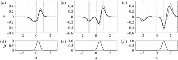
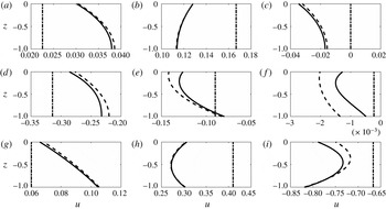
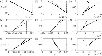
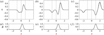
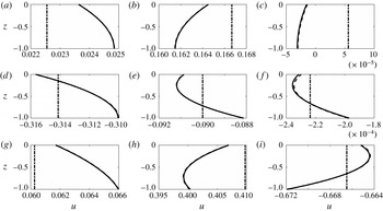
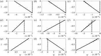
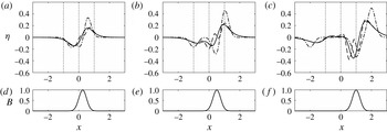
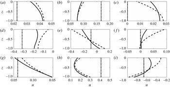
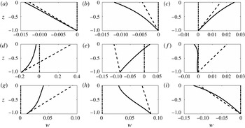
, the free-surface elevation solutions are compared in figure 7 and the velocity solutions are compared in figures 8 and 9. While LSWE is clearly inaccurate for this problem set-up, the LWD solutions overall agree well with the LFD solutions.
A case with a very long landslide,
 $\unicode[STIX]{x1D707}=0.05$
, in which all three models are accurate, as well as a case with a shorter landslide,
 $\unicode[STIX]{x1D707}=0.4$
, in which neither LSWE nor LWD is accurate, are shown in appendix D.
The free-surface elevation
 $\unicode[STIX]{x1D702}(x,t)$
at different times and locations, due to a moderately long Gaussian-shaped landslide with
 $\unicode[STIX]{x1D707}=0.2$
moving at speed
 $Fr=0.5$
: (a,d)
 $t=0.5$
; (b,e)
 $t=1.0$
; (c,f)
 $t=2.0$
; solid line, LFD solution (2.6); dashed line, LWD solution (2.22); dash–dot line, LSWE solution (1.3); dotted lines, locations at which the velocity solutions are shown.

The vertical distribution of the horizontal velocity
 $u(x,z,t)$
at different times and locations, due to a moderately long Gaussian-shaped landslide with
 $\unicode[STIX]{x1D707}=0.2$
moving at speed
 $Fr=0.5$
: (a,d,g)
 $t=0.5$
; (b,e,h)
 $t=1.0$
; (c,f,i)
 $t=2.0$
; (a–c)
 $x=-1$
; (d–f)
 $x=0$
; (g–i)
 $x=1$
; solid line, LFD solution (2.8); dashed line, LWD solution recovered from (2.25); dash–dot line, LSWE solution (1.4). It should be noted that the scale of the horizontal axis varies greatly from panel to panel.

The vertical distribution of the vertical velocity
 $w(x,z,t)$
at different times and locations, due to a moderately long Gaussian-shaped landslide with
 $\unicode[STIX]{x1D707}=0.2$
moving at speed
 $Fr=0.5$
: (a,d,g)
 $t=0.5$
; (b,e,h)
 $t=1.0$
; (c,f,i)
 $t=2.0$
; (a–c)
 $x=-1$
; (d–f)
 $x=0$
; (g–i)
 $x=1$
; solid line, LFD solution (2.9); dashed line, LWD solution recovered from (2.25); dash–dot line, LSWE solution (zero vertical velocity). It should be noted that the scale of the horizontal axis varies greatly from panel to panel.

3 Landslide-generated waves on a constant slope
3.1 One-dimensional (horizontal) LSWEs
The dimensionless 1DH LSWEs read
 $$\begin{eqnarray}\displaystyle \unicode[STIX]{x1D702}_{t}+(uh)_{x}=B_{t} & & \displaystyle\end{eqnarray}$$
and
 $$\begin{eqnarray}\displaystyle u_{t}=-\unicode[STIX]{x1D702}_{x}, & & \displaystyle\end{eqnarray}$$
where (
 $\unicode[STIX]{x1D702}$
,
 $B$
) are normalised by the landslide thickness
 $A$
,
 $x$
is normalised by the landslide length
 $L$
,
 $h=x\tan \unicode[STIX]{x1D703}$
, normalised by
 $L\tan \unicode[STIX]{x1D703}$
, is the still water depth on a constant slope of angle
 $\unicode[STIX]{x1D703}$
,
 $u$
is normalised by
 $A\sqrt{gL\tan \unicode[STIX]{x1D703}}/L\tan \unicode[STIX]{x1D703}$
and
 $t$
is normalised by
 $\sqrt{L/g\tan \unicode[STIX]{x1D703}}$
. The landslide forcing function
 $B$
is described in the water coordinate system (vertical–horizontal). The shoreline is located at
 $x=0$
and the physical domain of interest is
 $x>0$
.
Again, either
 $\unicode[STIX]{x1D702}$
or
 $u$
can be solved for first. To solve for
 $\unicode[STIX]{x1D702}$
first, equations (3.1) and (3.2) can be combined into
 $$\begin{eqnarray}\displaystyle x\unicode[STIX]{x1D702}_{xx}+\unicode[STIX]{x1D702}_{x}-\unicode[STIX]{x1D702}_{tt}=-B_{tt}. & & \displaystyle\end{eqnarray}$$
Tuck & Hwang (Reference Tuck and Hwang1972) first solved this equation using the Laplace and Hankel transforms to obtain the solution for
 $\unicode[STIX]{x1D702}$
. Here, we impose the initial conditions
 $$\begin{eqnarray}\displaystyle \unicode[STIX]{x1D702}(x,0)=0\quad \text{and}\quad \unicode[STIX]{x1D702}_{t}(x,0)=B_{t}(x,0), & & \displaystyle\end{eqnarray}$$
the latter resulting from setting
 $[u(x,0)h]_{x}=0$
in (3.1) – on a constant slope with
 $h=x\tan \unicode[STIX]{x1D703}$
, this corresponds to
 $u(x,0)=\text{const.}/x$
– and rederive the integral-form solution (valid for
 $x>0,t>0$
) as
 $$\begin{eqnarray}\displaystyle \unicode[STIX]{x1D702}(x,t)=2\int _{0}^{\infty }\text{J}_{0}(2\sqrt{\unicode[STIX]{x1D706}x})\int _{0}^{t}\cos \left(\sqrt{\unicode[STIX]{x1D706}}(t-\unicode[STIX]{x1D70F})\right)\int _{0}^{\infty }sB_{\unicode[STIX]{x1D70F}}(s^{2},\unicode[STIX]{x1D70F})\text{J}_{0}(2\sqrt{\unicode[STIX]{x1D706}}s)\,\text{d}s\,\text{d}\unicode[STIX]{x1D70F}\,\text{d}\unicode[STIX]{x1D706}, & & \displaystyle\end{eqnarray}$$
where
 $\text{J}_{0}$
is the Bessel function of the first kind with order
 $0$
. The solution for
 $u$
can then be recovered from (3.2) as
 $$\begin{eqnarray}\displaystyle u(x,t) & = & \displaystyle u(x,0)+\frac{2}{\sqrt{x}}\int _{0}^{\infty }\sqrt{\unicode[STIX]{x1D706}}\,\text{J}_{1}(2\sqrt{\unicode[STIX]{x1D706}x})\int _{0}^{t}\int _{0}^{\unicode[STIX]{x1D713}}\cos \left(\sqrt{\unicode[STIX]{x1D706}}(t-\unicode[STIX]{x1D70F})\right)\nonumber\\ \displaystyle & & \displaystyle \times \,\int _{0}^{\infty }sB_{\unicode[STIX]{x1D70F}}(s^{2},\unicode[STIX]{x1D70F})\text{J}_{0}(2\sqrt{\unicode[STIX]{x1D706}}s)\,\text{d}s\,\text{d}\unicode[STIX]{x1D70F}\,\text{d}\unicode[STIX]{x1D713}\,\text{d}\unicode[STIX]{x1D706}.\end{eqnarray}$$
The precise initial condition for the horizontal velocity,
 $u(x,0)$
, can be specified only when the solution for
 $u$
is considered; here, we require
 $u(x,0)=0$
for initially quiescent water.
While the solution for
 $\unicode[STIX]{x1D702}$
, equation (3.5), is in a slightly different form from that in Tuck & Hwang (Reference Tuck and Hwang1972), we have verified that the two solutions are indeed the same. Our goal is to seek special landslide forcing functions
 $B(x,t)$
that have closed-form integrals in (3.5). Liu et al. (Reference Liu, Lynett and Synolakis2003) showed that the use of a deforming Gaussian-like landslide moving at the same speed as the wave celerity reduces the number of integrals to one.
We consider a ramp-like landslide forcing function:
 $$\begin{eqnarray}\displaystyle B(x,t)=R(\unicode[STIX]{x1D6FD}t-\sqrt{x}), & & \displaystyle\end{eqnarray}$$
where
 $\unicode[STIX]{x1D6FD}$
is a constant to be chosen and
 $R$
is the ramp function, defined as
 $$\begin{eqnarray}\displaystyle R(\unicode[STIX]{x1D709})=\left\{\begin{array}{@{}c@{}}\unicode[STIX]{x1D709},\unicode[STIX]{x1D709}\geqslant 0,\\ 0,\unicode[STIX]{x1D709}<0.\end{array}\right. & & \displaystyle\end{eqnarray}$$
Thus, the temporal derivative of
 $B$
is
 $$\begin{eqnarray}\displaystyle B_{t}(x,t)=\unicode[STIX]{x1D6FD}H(\unicode[STIX]{x1D6FD}t-\sqrt{x}), & & \displaystyle\end{eqnarray}$$
where
 $H$
denotes the Heaviside step function. A closed-form Hankel transform is available for the step function (Poularikas Reference Poularikas2000), and equation (3.5) can be written as
 $$\begin{eqnarray}\displaystyle \unicode[STIX]{x1D702}(x,t) & = & \displaystyle \unicode[STIX]{x1D6FD}^{2}\int _{0}^{\infty }\frac{\text{J}_{0}(2\sqrt{\unicode[STIX]{x1D706}}\sqrt{x})}{\sqrt{\unicode[STIX]{x1D706}}}\left[\cos (\sqrt{\unicode[STIX]{x1D706}}t)\int _{0}^{t}\unicode[STIX]{x1D70F}\cos (\sqrt{\unicode[STIX]{x1D706}}\unicode[STIX]{x1D70F})\text{J}_{1}(2\unicode[STIX]{x1D6FD}\sqrt{\unicode[STIX]{x1D706}}\unicode[STIX]{x1D70F})\,\text{d}\unicode[STIX]{x1D70F}\right.\nonumber\\ \displaystyle & & \displaystyle +\left.\sin (\sqrt{\unicode[STIX]{x1D706}}t)\int _{0}^{t}\unicode[STIX]{x1D70F}\sin (\sqrt{\unicode[STIX]{x1D706}}\unicode[STIX]{x1D70F})\text{J}_{1}(2\unicode[STIX]{x1D6FD}\sqrt{\unicode[STIX]{x1D706}}\unicode[STIX]{x1D70F})\,\text{d}\unicode[STIX]{x1D70F}\right]\,\text{d}\unicode[STIX]{x1D706}.\end{eqnarray}$$
Furthermore, if we choose
 $\unicode[STIX]{x1D6FD}=1/2$
, the
 $\unicode[STIX]{x1D70F}$
-integrals can be evaluated (Rosenheinrich Reference Rosenheinrich2015), and the equation becomes
 $$\begin{eqnarray}\displaystyle \unicode[STIX]{x1D702}(x,t)=\frac{t^{2}}{12}\int _{0}^{\infty }\frac{\text{J}_{0}(2\sqrt{\unicode[STIX]{x1D706}}\sqrt{x})\text{J}_{1}(\sqrt{\unicode[STIX]{x1D706}}t)}{\sqrt{\unicode[STIX]{x1D706}}}\,\text{d}\unicode[STIX]{x1D706}=\frac{t^{2}}{12}\int _{0}^{\infty }\text{J}_{0}(\sqrt{x}\unicode[STIX]{x1D714})\text{J}_{1}\left(\frac{t}{2}\unicode[STIX]{x1D714}\right)\,\text{d}\unicode[STIX]{x1D714}. & & \displaystyle\end{eqnarray}$$
This last integral can also be evaluated (Gradshteyn & Ryzhik Reference Gradshteyn and Ryzhik2007), and we have simply
 $$\begin{eqnarray}\displaystyle \unicode[STIX]{x1D702}(x,t)=\frac{t}{6}H\left[-\!\left(\sqrt{x}-\frac{t}{2}\right)\right], & & \displaystyle\end{eqnarray}$$
which is a jump from
 $t/6$
to
 $0$
travelling along
 $x=t^{2}/4$
, where the front of the landslide is. Similarly to the landslide used in Liu et al. (Reference Liu, Lynett and Synolakis2003), the landslide accelerates so that it always travels at local wave speed. The solution for
 $u$
can be recovered from (3.2), with the initial condition
 $u(x,0)=0$
, as
 $$\begin{eqnarray}\displaystyle u(x,t)=\frac{1}{3}H\left[-\!\left(\sqrt{x}-\frac{t}{2}\right)\right], & & \displaystyle\end{eqnarray}$$
which is a step function whose amplitude does not change.
The analytical solution (3.12) serves as a challenging benchmark for numerical models, since it consists of a shock and a ‘shoreline’ (
 $x\rightarrow 0$
) in linear theory. To demonstrate this, we solved the dimensional 1DH LSWEs (3.1) and (3.2) using a finite-difference solver, which employs the fourth-order central difference scheme in space and the third-order strong stability preserving Runge–Kutta scheme in time (Gottlieb, Shu & Tadmor Reference Gottlieb, Shu and Tadmor2001). The open boundary condition (derivatives equal zero) is used on the right boundary. For the left (shoreline) boundary, linear extrapolation is used to acquire the surface elevations at the ghost points located at
 $x\leqslant 0$
, and the flow velocity at
 $x\leqslant 0$
is assumed to be zero, which are needed in computing the derivatives based on the central difference scheme. In addition, since the water depth at exactly
 $x=0$
is
 $0$
, the first point in the numerical model is actually located at
 $x=\unicode[STIX]{x0394}x$
, where
 $\unicode[STIX]{x0394}x$
is the grid spacing (normalised by the landslide length). Using two different grid spacings
 $\unicode[STIX]{x0394}x=0.01$
and
 $\unicode[STIX]{x0394}x=0.001$
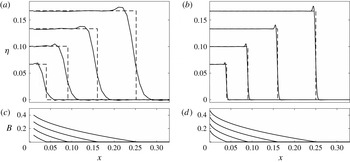
, we computed the numerical solution (normalised) due to the ramp-like landslide forcing function, and the comparison with the analytical solution is shown in figure 10. While the general location of the jump as well as the water surface elevations on the two sides of the jump are well captured, the width of the jump greatly depends on the grid spacing
 $\unicode[STIX]{x0394}x$
. Overshoot of the computed surface elevation is obvious near the jump, which is a common characteristic of the finite-difference scheme near sharp gradients. On the other hand, the numerical shoreline treatment seems to perform well in this problem, although small oscillations can still be observed in the free-surface elevations away from the jump.
Comparison of the numerical and analytical solutions of the 1DH LSWEs for a ramp-like landslide-generated wave on a constant slope at times
 $t=0.4,0.6,0.8,1$
; solid line, numerical solution; dashed line, analytical solution; (a,c) numerical solution with grid spacing
 $\unicode[STIX]{x0394}x=0.01$
; (b,d) numerical solution with grid spacing
 $\unicode[STIX]{x0394}x=0.001$
.

Even though the results presented in figure 10 appear to be satisfactory, it should be noted that the two grid spacings used in the example (
 $\unicode[STIX]{x0394}x=0.01$
and
 $\unicode[STIX]{x0394}x=0.001$
) are fairly fine and are impractical in larger simulation domains. Therefore, more sophisticated numerical methods are necessary to resolve the sharp gradient (jump) and the shoreline boundary with a more reasonably sized grid spacing in a numerical model based on linear theory, and the closed-form analytical solution (3.12) serves as a convenient tool to test the effectiveness of the numerical methods.
3.2 Two-dimensional (horizontal) LSWEs
The dimensionless 2DH LSWEs read
 $$\begin{eqnarray}\displaystyle \unicode[STIX]{x1D702}_{t}+(uh)_{x}+(vh)_{y}=B_{t}, & & \displaystyle\end{eqnarray}$$
 $$\begin{eqnarray}\displaystyle u_{t}=-\unicode[STIX]{x1D702}_{x},\quad v_{t}=-\unicode[STIX]{x1D702}_{y}, & & \displaystyle\end{eqnarray}$$
where the notations are the same as those in (3.1) and (3.2), with the addition of
 $v(x,y,t)$
, the horizontal water velocity in the
 $y$
-direction. On a plane beach of angle
 $\unicode[STIX]{x1D703}$
with the shoreline located at
 $x=0$
so that
 $y$
is in the longshore direction, the physical domain of interest is
 $x>0$
and the still water depth is
 $h(x,y)=x\tan \unicode[STIX]{x1D703}$
. Combining the equations to solve for
 $\unicode[STIX]{x1D702}$
first, we obtain
 $$\begin{eqnarray}\displaystyle \unicode[STIX]{x1D702}_{tt}-x\unicode[STIX]{x1D702}_{xx}-\unicode[STIX]{x1D702}_{x}-x\unicode[STIX]{x1D702}_{yy}=B_{tt}. & & \displaystyle\end{eqnarray}$$
We seek the analytical solution to (3.16). It should be noted that, like in the 1DH case, the landslide forcing function
 $B(x,y,t)$
is described in the water coordinate system (vertical–horizontal).
The analytical solution to (3.16) for the landslide-wave problem, valid for
 $x>0,t>0$
, was first obtained in Sammarco & Renzi (Reference Sammarco and Renzi2008) and Renzi (Reference Renzi2010) with the initial conditions
 $\unicode[STIX]{x1D702}(x,y,0)=0$
and
 $\unicode[STIX]{x1D702}_{t}(x,y,0)=0$
, for any landslide forcing function symmetric about the
 $x$
-axis. However, we note that the initial condition
 $\unicode[STIX]{x1D702}_{t}(x,y,0)=0$
does not fulfil the quiescent water condition in the LSWEs and would result in initial water velocities that depend on
 $B_{t}(x,y,0)$
(which can be non-zero): by setting
 $\unicode[STIX]{x1D702}_{t}(x,y,0)=0$
in (3.14), we obtain
 $[u(x,y,0)h]_{x}+[v(x,y,0)h]_{y}=B_{t}(x,y,0)$
; under this condition,
 $u(x,y,0)=0=v(x,y,0)$
is not possible for
 $B_{t}(x,y,0)\neq 0$
.
Similarly to the 1DH cases discussed previously, when solving for
 $\unicode[STIX]{x1D702}$
first, to allow for the quiescent water condition, the initial conditions that should be imposed are
 $$\begin{eqnarray}\displaystyle \unicode[STIX]{x1D702}(x,y,0)=0\quad \text{and}\quad \unicode[STIX]{x1D702}_{t}(x,y,0)=B_{t}(x,y,0), & & \displaystyle\end{eqnarray}$$
the latter resulting from setting
 $[u(x,y,0)h]_{x}+[v(x,y,0)h]_{y}=0$
in (3.14), which allows for the possibility that
 $u(x,y,0)=0=v(x,y,0)$
. The precise initial velocities,
 $u(x,y,0)$
and
 $v(x,y,0)$
, can be specified only when the solutions for
 $u(x,y,t)$
and
 $v(x,y,t)$
are considered. It should be noted that the two different initial conditions used, i.e.
 $\unicode[STIX]{x1D702}_{t}(x,y,0)=0$
and
 $\unicode[STIX]{x1D702}_{t}(x,y,0)=B_{t}(x,y,0)$
, become identical only when a landslide forcing function with
 $B_{t}(x,y,0)=0$
is chosen.
We rederive the analytical solution using the new initial conditions and obtain
 $$\begin{eqnarray}\displaystyle & & \displaystyle \unicode[STIX]{x1D702}(x,y,t)=2\sqrt{\frac{2}{\unicode[STIX]{x03C0}}}\mathop{\sum }_{n=0}^{\infty }\int _{0}^{\infty }L_{n}(2kx)k\text{e}^{-kx}\cos (ky)\int _{0}^{\infty }L_{n}(2ks)\text{e}^{-ks}\nonumber\\ \displaystyle & & \displaystyle \quad \times \,\left[\overline{B}(s,k,t)-\cos (\sqrt{\unicode[STIX]{x1D706}}t)\overline{B}(s,k,0)-\sqrt{\unicode[STIX]{x1D706}}\int _{0}^{t}\sin \left(\sqrt{\unicode[STIX]{x1D706}}(t-\unicode[STIX]{x1D70F})\right)\overline{B}(s,k,\unicode[STIX]{x1D70F})\,\text{d}\unicode[STIX]{x1D70F}\right]\,\text{d}s\,\text{d}k,\nonumber\\ \displaystyle & & \displaystyle\end{eqnarray}$$
where
 $L_{n}(x)$
is the
 $n$
th-order Laguerre polynomial,
 $\overline{B}$
is the Fourier-transformed
 $B$
with respect to
 $y$
(
 $B$
is assumed to be symmetric about the
 $x$
-axis) and
 $\unicode[STIX]{x1D706}=k(2n+1)$
. The velocity solutions based on the new solution for
 $\unicode[STIX]{x1D702}$
, equation (3.18), can be recovered from the momentum equation (3.15) as
 $$\begin{eqnarray}\displaystyle & & \displaystyle u(x,y,t)=u(x,y,0)\nonumber\\ \displaystyle & & \displaystyle \quad +\,2\sqrt{\frac{2}{\unicode[STIX]{x03C0}}}\mathop{\sum }_{n=0}^{\infty }\int _{0}^{\infty }L_{n}(2kx)k^{2}\text{e}^{-kx}\cos (ky)\int _{0}^{\infty }L_{n}(2ks)\text{e}^{-ks}\left[\int _{0}^{t}\overline{B}(s,k,\unicode[STIX]{x1D713})\,\text{d}\unicode[STIX]{x1D713}\right.\nonumber\\ \displaystyle & & \displaystyle \quad -\left.\frac{1}{\sqrt{\unicode[STIX]{x1D706}}}\sin (\sqrt{\unicode[STIX]{x1D706}}t)\overline{B}(s,k,0)-\sqrt{\unicode[STIX]{x1D706}}\int _{0}^{t}\int _{0}^{\unicode[STIX]{x1D713}}\sin \left(\sqrt{\unicode[STIX]{x1D706}}(\unicode[STIX]{x1D713}-\unicode[STIX]{x1D70F})\right)\overline{B}(s,k,\unicode[STIX]{x1D70F})\,\text{d}\unicode[STIX]{x1D70F}\,\text{d}\unicode[STIX]{x1D713}\right]\,\text{d}s\,\text{d}k\nonumber\\ \displaystyle & & \displaystyle \quad +\,4\sqrt{\frac{2}{\unicode[STIX]{x03C0}}}\mathop{\sum }_{n=1}^{\infty }\int _{0}^{\infty }L_{n-1}^{(1)}(2kx)k^{2}\text{e}^{-kx}\cos (ky)\int _{0}^{\infty }L_{n}(2ks)\text{e}^{-ks}\left[\int _{0}^{t}\overline{B}(s,k,\unicode[STIX]{x1D713})\,\text{d}\unicode[STIX]{x1D713}\right.\nonumber\\ \displaystyle & & \displaystyle \quad -\left.\frac{1}{\sqrt{\unicode[STIX]{x1D706}}}\sin (\sqrt{\unicode[STIX]{x1D706}}t)\overline{B}(s,k,0)-\sqrt{\unicode[STIX]{x1D706}}\int _{0}^{t}\int _{0}^{\unicode[STIX]{x1D713}}\sin \left(\sqrt{\unicode[STIX]{x1D706}}(\unicode[STIX]{x1D713}-\unicode[STIX]{x1D70F})\right)\overline{B}(s,k,\unicode[STIX]{x1D70F})\,\text{d}\unicode[STIX]{x1D70F}\,\text{d}\unicode[STIX]{x1D713}\right]\,\text{d}s\,\text{d}k\nonumber\\ \displaystyle & & \displaystyle\end{eqnarray}$$
and
 $$\begin{eqnarray}\displaystyle & & \displaystyle v(x,y,t)=v(x,y,0)\nonumber\\ \displaystyle & & \displaystyle \quad +\,2\sqrt{\frac{2}{\unicode[STIX]{x03C0}}}\mathop{\sum }_{n=0}^{\infty }\int _{0}^{\infty }L_{n}(2kx)k^{2}\text{e}^{-kx}\sin (ky)\int _{0}^{\infty }L_{n}(2ks)\text{e}^{-ks}\left[\int _{0}^{t}\overline{B}(s,k,\unicode[STIX]{x1D713})\,\text{d}\unicode[STIX]{x1D713}\right.\nonumber\\ \displaystyle & & \displaystyle \quad -\left.\frac{1}{\sqrt{\unicode[STIX]{x1D706}}}\sin (\sqrt{\unicode[STIX]{x1D706}}t)\overline{B}(s,k,0)-\sqrt{\unicode[STIX]{x1D706}}\int _{0}^{t}\int _{0}^{\unicode[STIX]{x1D713}}\sin \left(\sqrt{\unicode[STIX]{x1D706}}(\unicode[STIX]{x1D713}-\unicode[STIX]{x1D70F})\right)\overline{B}(s,k,\unicode[STIX]{x1D70F})\,\text{d}\unicode[STIX]{x1D70F}\,\text{d}\unicode[STIX]{x1D713}\right]\,\text{d}s\,\text{d}k.\nonumber\\ \displaystyle & & \displaystyle\end{eqnarray}$$
For initially quiescent water, we further require
 $u(x,y,0)=0=v(x,y,0)$
, in addition to the initial conditions already imposed when solving for
 $\unicode[STIX]{x1D702}$
, i.e.
 $\unicode[STIX]{x1D702}(x,y,0)=0$
and
 $[u(x,y,0)h]_{x}+[v(x,y,0)h]_{y}=0$
.
The analytical solutions in all existing studies (e.g. Sammarco & Renzi Reference Sammarco and Renzi2008; Renzi Reference Renzi2010; Renzi & Sammarco Reference Renzi and Sammarco2010, Reference Renzi and Sammarco2012; Seo & Liu Reference Seo and Liu2013) include an extra term in addition to (3.18) due to non-zero initial water velocities:
 $$\begin{eqnarray}\displaystyle \unicode[STIX]{x1D702}_{extra}(x,y,t) & = & \displaystyle 2\sqrt{\frac{2}{\unicode[STIX]{x03C0}}}\mathop{\sum }_{n=0}^{\infty }\int _{0}^{\infty }L_{n}(2kx)k\text{e}^{-kx}\cos (ky)\int _{0}^{\infty }L_{n}(2ks)\text{e}^{-ks}\nonumber\\ \displaystyle & & \displaystyle \times \,\left[-\frac{\overline{B}_{t}(s,k,0)\sin (\sqrt{\unicode[STIX]{x1D706}}t)}{\sqrt{\unicode[STIX]{x1D706}}}\right]\,\text{d}s\,\text{d}k.\end{eqnarray}$$
Therefore, in this study, we only need to focus on the term (3.21) to evaluate how it affects previous findings. Clearly, the extra term vanishes if a landslide forcing function with
 $B_{t}(x,y,0)=0$
is used.
To examine the significance of
 $\unicode[STIX]{x1D702}_{extra}$
, we follow the asymptotic analysis discussed in Sammarco & Renzi (Reference Sammarco and Renzi2008), Renzi (Reference Renzi2010) and Seo & Liu (Reference Seo and Liu2013), and find the large-
 $t$
asymptotic approximation of
 $\unicode[STIX]{x1D702}_{extra}$
for
 $y>0$
to be
 $$\begin{eqnarray}\displaystyle \unicode[STIX]{x1D702}_{extra}(x,y,t)\simeq 2\mathop{\sum }_{n=0}^{\infty }L_{n}(2k_{0}x)\text{e}^{-k_{0}x}\left(\frac{1}{t|\unicode[STIX]{x1D714}_{0}^{\prime \prime }|}\right)^{1/2}C_{n}\sin \left(k_{0}y-\unicode[STIX]{x1D714}_{0}t+\frac{\unicode[STIX]{x03C0}}{4}\right),\quad t\rightarrow \infty , & & \displaystyle \nonumber\\ \displaystyle & & \displaystyle\end{eqnarray}$$
where
 $$\begin{eqnarray}\displaystyle \left.\begin{array}{@{}c@{}}\displaystyle k_{0}=\frac{2n+1}{4}\left(\frac{t}{y}\right)^{2},\quad \unicode[STIX]{x1D714}_{0}=\sqrt{k_{0}(2n+1)},\quad \unicode[STIX]{x1D714}_{0}^{\prime \prime }=-\frac{\sqrt{k_{0}(2n+1)}}{4k_{0}^{2}},\\ \displaystyle C_{n}=\frac{k_{0}}{\unicode[STIX]{x1D714}_{0}}\int _{0}^{\infty }L_{n}(2k_{0}s)\text{e}^{-k_{0}s}\overline{B_{t}}(s,k_{0},0)\,\text{d}s.\end{array}\right\} & & \displaystyle\end{eqnarray}$$
Equation (3.22) is the extra term included in the asymptotic solution in previous studies. It has the same form as a part of the asymptotic approximation of the true solution (3.18), the key difference being the
 $C_{n}$
term. Similar terms exist in the asymptotic approximation of (3.18). These terms need to be numerically evaluated and may depend on time, but in general their amplitudes do not grow in time for the translating landslide forcing functions considered in both previous studies and the present study. Therefore, while the asymptotic decay rate
 $t^{-1/2}$
remains the same, the exact wave shape can be very different due to the difference in the initial conditions used.
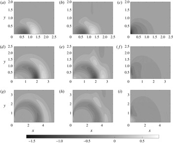
Wave fields generated by a double-Gaussian landslide forcing function moving at a constant speed
 $1$
from
 $x=0$
. The solution is symmetric about the
 $x$
-axis. (a,d,g) Numerical solution with
 $\unicode[STIX]{x0394}x=\unicode[STIX]{x0394}y=0.01$
; (b,e,h)
 $50$
-mode analytical solution; (c,f,i)
 $50$
-mode
 $\unicode[STIX]{x1D702}_{extra}$
; (a–c)
 $t=1$
; (d–f)
 $t=2$
; (g–i)
 $t=3$
.

In previous studies, translating landslides moving at a constant speed, for which
 $B_{t}(x,y,0)\neq 0$
, were used in plotting and further examining the solutions. Choosing as an example a double-Gaussian landslide forcing function moving at a constant speed
 $1$
from
 $x=0$
, i.e.
 $B(x,y,t)=\text{e}^{-8(x-t)^{2}}\text{e}^{-8y^{2}}$
, we solved the 2DH LSWEs numerically using a similar numerical model to that described in the previous section (with a fairly fine grid spacing of
 $\unicode[STIX]{x0394}x=\unicode[STIX]{x0394}y=0.01$
), and compare the results with the
 $50$
-mode analytical solution (3.18) evaluated with numerical integration methods described by Seo & Liu (Reference Seo and Liu2013). The resulting free-surface elevations at
 $t=1,2,3$
are shown in figure 11. Although the numerical solution of the LSWEs can be problematic near the shoreline, it is robust and reliable away from the shoreline. Since the integral-form analytical solution requires further numerical evaluation and approximation in plotting, in this case, the numerical solution is a better choice as the reference solution when the overall wave field (i.e. not the edge waves) is of concern, such as those shown in figure 11. While the numerically evaluated analytical solutions generally agree well with the numerical solutions, some oscillations are clearly visible (e.g. along
 $y=2$
at
 $t=2$
). On the other hand, we see that in this example the magnitude of
 $\unicode[STIX]{x1D702}_{extra}$
is always significant when compared with the true solution, suggesting that its impact on the true solution is not negligible.
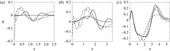
Analytical solutions of the free-surface elevation along
 $y=2$
due to a double-Gaussian landslide forcing function moving at a constant speed
 $1$
from
 $x=0$
: solid line, numerical solution with
 $\unicode[STIX]{x0394}x=\unicode[STIX]{x0394}y=0.01$
; dashed line,
 $6$
-mode analytical solution; dash–dot line,
 $10$
-mode analytical solution; dotted line,
 $50$
-mode analytical solution; (a)
 $t=1$
; (b)
 $t=2$
; (c)
 $t=3$
.

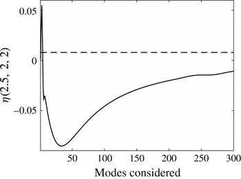
Plot examining the convergence rate of the analytical solution for
 $\unicode[STIX]{x1D702}(2.5,2,2)$
: solid line, analytical solution as a function of the number of modes considered; dashed line, numerical solution.

Upon closer inspection of the oscillations observed in the analytical solutions in figure 11, we found the cause to be a poor convergence rate of the analytical solution with respect to the number of modes considered in (3.18). To highlight this issue, we focus on the wave profile along
 $y=2$
in figure 11, which appears to be highly problematic, and compare in figure 12 the numerical solution with analytical solutions computed using different numbers of modes. We see that in this case, convergence of the solution is not reached even with
 $50$
modes considered. To further examine the convergence rate, in figure 13 we pick a point
 $(x,y,t)=(2.5,2,2)$
and plot
 $\unicode[STIX]{x1D702}(2.5,2,2)$
as a function of the number of modes considered. Based on figure 11, this point is situated ahead of the leading wave. We thus expect a very small value here – the numerical solution predicts
 $\unicode[STIX]{x1D702}(2.5,2,2)\simeq 0.008$
, yet the analytical solution is still only slowly converging even with 300 modes considered. We remark that the numerical integration can be time-consuming, and it is often undesirable to consider more than
 ${\sim}20$
modes. As a reference, Sammarco & Renzi (Reference Sammarco and Renzi2008) and Renzi (Reference Renzi2010) mostly considered only the first six modes, and Seo & Liu (Reference Seo and Liu2013) considered only the first 10 modes.
The analytical solution shines when the edge waves that propagate along
 $x=0$
or large-time/far-field solutions are of interest, where accurate numerical solutions are difficult to obtain. As mentioned previously, the numerical shoreline boundary treatment in linear theory is problematic. In addition, computational cost can be significant when the far-field or large-time solution is wanted, since numerical simulations have to resolve the entire domain starting from
 $t=0$
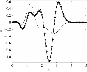
. Analytical solution is thus highly preferable in these situations. To examine the edge wave solutions more closely, in figure 14 we compare the analytical solutions with the numerical solution for the same double-Gaussian landslide forcing function case along
 $(x,y,t)=(0,y,5)$
. In this case, we find the
 $10$
-mode analytical solution to be nearly identical to the
 $15$
-mode solution, suggesting that consideration of the first
 $10$
modes is sufficient in this case (while not shown here, six modes are still insufficient in this example). We therefore advise that a convergence test be performed every time the analytical solution is used at a different location, to ensure that satisfactory convergence is reached within a reasonable number of modes considered. In figure 14, we also included
 $\unicode[STIX]{x1D702}_{extra}$
, and see that its amplitude is significant, again showing its permanent effect on the wave shape. On the other hand, even with the fine grid spacing
 $\unicode[STIX]{x0394}x=\unicode[STIX]{x0394}y=0.01$
, the numerical edge wave solutions still do not fully agree with the analytical solutions, which in this case have converged and should be regarded as the reference solution.
Edge waves (
 $x=0$
) at
 $t=5$
due to a double-Gaussian landslide forcing function moving at a constant speed
 $1$
from
 $x=0$
: solid line, numerical solution with
 $\unicode[STIX]{x0394}x=\unicode[STIX]{x0394}y=0.01$
; plus,
 $10$
-mode analytical solution; circle,
 $15$
-mode analytical solution; dashed line,
 $15$
-mode
 $\unicode[STIX]{x1D702}_{extra}$
.

4 Concluding remarks
In this study, we revisited the analytical solutions, for both the free-surface elevation and the flow velocity, for various landslide-generated wave problems. One-dimensional (horizontal) analytical solutions for water waves generated by a solid landslide moving at a constant speed in constant water depth were obtained for the linear and weakly dispersive model as well as the linear and fully dispersive model. We further used the 1DH linear and fully dispersive model in constant depth to show that the area enclosed by the landslide has stronger lasting effects on the generated water waves than the exact landslide shape; in experiments and numerical simulations it is therefore more important to match the enclosed area and the characteristic landslide scales than the exact shape. In addition, we employed the linear and fully dispersive model to show that the resonance (
 $Fr=1$
) leading-wave solution grows at the rate
 $t^{1/3}$
, instead of decaying at the rate
 $t^{-1/3}$
for
 $Fr\neq 1$
. For the 1DH LSWEs on a constant slope, we found a closed-form solution containing a ‘shoreline’ in linear theory and a shock propagating at the same speed as the local wave speed. This solution could serve as a challenging benchmark for numerical models since the numerical treatment of a shoreline boundary in linear theory and the preservation of sharp gradients can be problematic. For the 2DH LSWEs on a plane beach, we showed that the initial conditions used in previous studies result in initial water velocities that can be non-zero, rederived the solution using quiescent water initial conditions consistent with the governing equations, and found that the difference in the initial conditions has a permanent effect on the generated waves. In addition, we pointed out that the numerical evaluation of the analytical solution is not always rapidly converging, and advised that a case-by-case convergence test be performed to ensure the accuracy of the computed analytical solution.
The solution procedure introduced in this paper is being extended to find solutions for 2DH constant depth with a broader application. New results are forthcoming.
Acknowledgements
We would like to acknowledge the support from Cornell University. P.L.-F.L. would like to acknowledge the support from the National University of Singapore. The authors are grateful for the anonymous reviewers’ constructive feedback, which has greatly increased the depth of this study.
Appendix A. Landslide shape definitions
The (dimensionless) Gaussian-shaped landslide is defined so that the characteristic length is four standard deviations (thus,
 ${\sim}95\,\%$
of the area is contained in one characteristic length):
 $$\begin{eqnarray}\displaystyle B_{1}(x-Fr\,t)=\text{e}^{-8(x-Fr\,t)^{2}}. & & \displaystyle\end{eqnarray}$$
The area enclosed is
 $S_{B}=\sqrt{\unicode[STIX]{x03C0}/2}/2$
and the Fourier transform is
 $$\begin{eqnarray}\displaystyle \overline{B_{1}}={\textstyle \frac{1}{4}}\text{e}^{-(1/32)k^{2}}\text{e}^{-\text{i}kFr\,t}. & & \displaystyle\end{eqnarray}$$
The landslide shape can also be a parabolic cap of the same height and enclosed area:
 $$\begin{eqnarray}\displaystyle B_{2}(x-Fr\,t) & = & \displaystyle \left[H\left(x-Fr\,t+\frac{3}{8}\sqrt{\frac{\unicode[STIX]{x03C0}}{2}}\right)-H\left(x-Fr\,t-\frac{3}{8}\sqrt{\frac{\unicode[STIX]{x03C0}}{2}}\right)\right]\nonumber\\ \displaystyle & & \displaystyle \times \,\left[1-\frac{128}{9\unicode[STIX]{x03C0}}(x-Fr\,t)^{2}\right],\end{eqnarray}$$
where
 $H(x)$
is the Heaviside step function. Differently from the Gaussian curve, the parabolic cap has a finite length of
 $3\sqrt{\unicode[STIX]{x03C0}/2}/4$
. A closed-form Fourier transform is available for this landslide forcing function:
 $$\begin{eqnarray}\displaystyle \overline{B_{2}} & = & \displaystyle \bigg[-\frac{16}{3\unicode[STIX]{x03C0}k^{2}}(\text{e}^{-\text{i}(3/8)\sqrt{(\unicode[STIX]{x03C0}/2)}k}+\text{e}^{\text{i}(3/8)\sqrt{(\unicode[STIX]{x03C0}/2)}k})\nonumber\\ \displaystyle & & \displaystyle +\,\text{i}\frac{128\sqrt{2}}{9\unicode[STIX]{x03C0}^{3/2}k^{3}}(\text{e}^{-\text{i}(3/8)\sqrt{(\unicode[STIX]{x03C0}/2)}k}-\text{e}^{\text{i}(3/8)\sqrt{(\unicode[STIX]{x03C0}/2)}k})\bigg]\text{e}^{-\text{i}kFr\,t}.\end{eqnarray}$$
Similarly, a quartic cap can be used:
 $$\begin{eqnarray}\displaystyle B_{3}(x-Fr\,t) & = & \displaystyle \left[H\left(x-Fr\,t+\frac{5}{16}\sqrt{\frac{\unicode[STIX]{x03C0}}{2}}\right)-H\left(x-Fr\,t-\frac{5}{16}\sqrt{\frac{\unicode[STIX]{x03C0}}{2}}\right)\right]\nonumber\\ \displaystyle & & \displaystyle \times \,\left[1-\left(\frac{512}{25\unicode[STIX]{x03C0}}\right)^{2}(x-Fr\,t)^{4}\right],\end{eqnarray}$$
which has a finite length
 $5\sqrt{\unicode[STIX]{x03C0}/2}/8$
and whose Fourier transform is
 $$\begin{eqnarray}\displaystyle \overline{B_{3}} & = & \displaystyle \left[\frac{64}{125\unicode[STIX]{x03C0}^{2}k^{4}}(3072-25\unicode[STIX]{x03C0}k^{2})(\text{e}^{-\text{i}(5/16)\sqrt{(\unicode[STIX]{x03C0}/2)}k}+\text{e}^{\text{i}(5/16)\sqrt{(\unicode[STIX]{x03C0}/2)}k})\right.\nonumber\\ \displaystyle & & \displaystyle -\left.\text{i}\frac{1024\sqrt{2}}{625\unicode[STIX]{x03C0}^{5/2}k^{5}}(3072-75\unicode[STIX]{x03C0}k^{2})(\text{e}^{-\text{i}(5/16)\sqrt{(\unicode[STIX]{x03C0}/2)}k}-\text{e}^{\text{i}(5/16)\sqrt{(\unicode[STIX]{x03C0}/2)}k})\right]\text{e}^{-\text{i}kFr\,t}.\end{eqnarray}$$
Simple geometry such as a rectangle is also considered:
 $$\begin{eqnarray}\displaystyle B_{4}(x-Fr\,t)=H\left(x-Fr\,t+\frac{\sqrt{2\unicode[STIX]{x03C0}}}{8}\right)-H\left(x-Fr\,t-\frac{\sqrt{2\unicode[STIX]{x03C0}}}{8}\right), & & \displaystyle\end{eqnarray}$$
which has a finite length
 $\sqrt{2\unicode[STIX]{x03C0}}/4$
and Fourier transform
 $$\begin{eqnarray}\displaystyle \overline{B_{4}}=\text{i}\frac{1}{\sqrt{2\unicode[STIX]{x03C0}}k}(\text{e}^{-\text{i}(\sqrt{2\unicode[STIX]{x03C0}}/8)k}-\text{e}^{\text{i}(\sqrt{2\unicode[STIX]{x03C0}}/8)k})\text{e}^{-\text{i}kFr\,t}. & & \displaystyle\end{eqnarray}$$
For an isosceles triangle,
 $$\begin{eqnarray}\displaystyle & & \displaystyle B_{5}(x-Fr\,t)=\left[1+\frac{4}{\sqrt{2\unicode[STIX]{x03C0}}}(x-Fr\,t)\right]\left[H\left(x-Fr\,t+\frac{\sqrt{2\unicode[STIX]{x03C0}}}{4}\right)-H(x-Fr\,t)\right]\nonumber\\ \displaystyle & & \displaystyle \quad +\left[1-\frac{4}{\sqrt{2\unicode[STIX]{x03C0}}}(x-Fr\,t)\right]\left[H\left(x-Fr\,t\right)-H\left(x-Fr\,t-\frac{\sqrt{2\unicode[STIX]{x03C0}}}{4}\right)\right],\end{eqnarray}$$
which has a finite length
 $\sqrt{2\unicode[STIX]{x03C0}}/2$
and Fourier transform
 $$\begin{eqnarray}\displaystyle \overline{B_{5}}=\frac{2}{\unicode[STIX]{x03C0}k^{2}}(2-\text{e}^{-\text{i}(\sqrt{2\unicode[STIX]{x03C0}}/4)k}-\text{e}^{\text{i}(\sqrt{2\unicode[STIX]{x03C0}}/4)k})\text{e}^{-\text{i}kFr\,t}. & & \displaystyle\end{eqnarray}$$
The shape
 $B_{6}$
is a right triangle with a positive slope,
 $$\begin{eqnarray}\displaystyle B_{6}(x-Fr\,t) & = & \displaystyle \left[\frac{2}{3}+\frac{2}{\sqrt{2\unicode[STIX]{x03C0}}}(x-Fr\,t)\right]\nonumber\\ \displaystyle & & \displaystyle \times \left[H\left(x-Fr\,t+\frac{\sqrt{2\unicode[STIX]{x03C0}}}{3}\right)-H\left(x-Fr\,t-\frac{\sqrt{2\unicode[STIX]{x03C0}}}{6}\right)\right],\end{eqnarray}$$
whose Fourier transform is
 $$\begin{eqnarray}\displaystyle \overline{B_{6}}=\left[\frac{1}{\unicode[STIX]{x03C0}k^{2}}(\text{e}^{-\text{i}(\sqrt{2\unicode[STIX]{x03C0}}/6)k}-\text{e}^{\text{i}(\sqrt{2\unicode[STIX]{x03C0}}/3)k})+\text{i}\frac{1}{\sqrt{2\unicode[STIX]{x03C0}}k}\text{e}^{-\text{i}(\sqrt{2\unicode[STIX]{x03C0}}/6)k}\right]\text{e}^{-\text{i}kFr\,t}. & & \displaystyle\end{eqnarray}$$
The shape
 $B_{7}$
is a right triangle with a negative slope,
 $$\begin{eqnarray}\displaystyle B_{7}(x-Fr\,t) & = & \displaystyle \left[\frac{2}{3}-\frac{2}{\sqrt{2\unicode[STIX]{x03C0}}}(x-Fr\,t)\right]\nonumber\\ \displaystyle & & \displaystyle \times \left[H\left(x-Fr\,t+\frac{\sqrt{2\unicode[STIX]{x03C0}}}{6}\right)-H\left(x-Fr\,t-\frac{\sqrt{2\unicode[STIX]{x03C0}}}{3}\right)\right],\end{eqnarray}$$
whose Fourier transform is
 $$\begin{eqnarray}\displaystyle \overline{B_{7}}=\left[\frac{1}{\unicode[STIX]{x03C0}k^{2}}(-\text{e}^{-\text{i}(\sqrt{2\unicode[STIX]{x03C0}}/3)k}+\text{e}^{\text{i}(\sqrt{2\unicode[STIX]{x03C0}}/6)k})+\text{i}\frac{1}{\sqrt{2\unicode[STIX]{x03C0}}k}\text{e}^{\text{i}(\sqrt{2\unicode[STIX]{x03C0}}/6)k}\right]\text{e}^{-\text{i}kFr\,t}. & & \displaystyle\end{eqnarray}$$
Appendix B. Resonance in the LFD
In the complete LFD solution (2.6), discontinuities exist in the expressions for
 $\unicode[STIX]{x1D702}_{_{Fr}}$
and
 $\unicode[STIX]{x1D702}_{+}$
when
 $k=k^{\ast }$
so that
 $D(\unicode[STIX]{x1D707}k^{\ast })=Fr$
:
 $$\begin{eqnarray}\displaystyle & \displaystyle \unicode[STIX]{x1D702}_{_{Fr}}(x,t)=-\frac{1}{\sqrt{2\unicode[STIX]{x03C0}}}\int _{-\infty }^{\infty }\frac{1}{\cosh \unicode[STIX]{x1D707}k}\frac{Fr^{2}}{D^{2}-Fr^{2}}\overline{B(x,0)}(k)\text{e}^{-\text{i}kFr\,t}\text{e}^{\text{i}kx}\,\text{d}k, & \displaystyle\end{eqnarray}$$
 $$\begin{eqnarray}\displaystyle & \displaystyle \unicode[STIX]{x1D702}_{+}(x,t)=\frac{1}{\sqrt{2\unicode[STIX]{x03C0}}}\int _{-\infty }^{\infty }\frac{1}{\cosh \unicode[STIX]{x1D707}k}\frac{Fr}{2(D-Fr)}\overline{B(x,0)}(k)\text{e}^{-\text{i}kDt}\text{e}^{\text{i}kx}\,\text{d}k, & \displaystyle\end{eqnarray}$$
 $$\begin{eqnarray}\displaystyle & \displaystyle D=\sqrt{\frac{\tanh \unicode[STIX]{x1D707}k}{\unicode[STIX]{x1D707}k}}. & \displaystyle\end{eqnarray}$$
It should be recalled that
 $D$
is a smooth function with a peak of one at
 $k=0$
(plotted in figure 2 as a function of
 $\unicode[STIX]{x1D707}k$
). Here, we show only the analysis for the discontinuity in
 $\unicode[STIX]{x1D702}_{+}$
. A similar analysis can be repeated for
 $\unicode[STIX]{x1D702}_{_{Fr}}$
.
To isolate the discontinuity at
 $k=k^{\ast }$
, we write
 $$\begin{eqnarray}\displaystyle \unicode[STIX]{x1D702}_{+}(x,t) & = & \displaystyle \lim _{\unicode[STIX]{x1D6FF}\rightarrow 0}\left\{\frac{1}{\sqrt{2\unicode[STIX]{x03C0}}}\int _{-\infty }^{k^{\ast }-\unicode[STIX]{x1D6FF}}\frac{1}{\cosh \unicode[STIX]{x1D707}k}\frac{Fr}{2(D-Fr)}\overline{B(x,0)}(k)\text{e}^{-\text{i}kDt}\text{e}^{\text{i}kx}\,\text{d}k\right.\nonumber\\ \displaystyle & & \displaystyle +\,\frac{1}{\sqrt{2\unicode[STIX]{x03C0}}}\int _{k^{\ast }-\unicode[STIX]{x1D6FF}}^{k^{\ast }+\unicode[STIX]{x1D6FF}}\frac{1}{\cosh \unicode[STIX]{x1D707}k}\frac{Fr}{2(D-Fr)}\overline{B(x,0)}(k)\text{e}^{-\text{i}kDt}\text{e}^{\text{i}kx}\,\text{d}k\nonumber\\ \displaystyle & & \displaystyle +\left.\frac{1}{\sqrt{2\unicode[STIX]{x03C0}}}\int _{k^{\ast }+\unicode[STIX]{x1D6FF}}^{\infty }\frac{1}{\cosh \unicode[STIX]{x1D707}k}\frac{Fr}{2(D-Fr)}\overline{B(x,0)}(k)\text{e}^{-\text{i}kDt}\text{e}^{\text{i}kx}\,\text{d}k\right\}.\end{eqnarray}$$
We therefore only need to focus on the term
 $$\begin{eqnarray}\displaystyle I(x,t)=\lim _{\unicode[STIX]{x1D6FF}\rightarrow 0}\left\{\frac{1}{\sqrt{2\unicode[STIX]{x03C0}}}\int _{k^{\ast }-\unicode[STIX]{x1D6FF}}^{k^{\ast }+\unicode[STIX]{x1D6FF}}\frac{1}{\cosh \unicode[STIX]{x1D707}k}\frac{Fr}{2(D-Fr)}\overline{B(x,0)}(k)\text{e}^{-\text{i}kDt}\text{e}^{\text{i}kx}\,\text{d}k\right\}. & & \displaystyle\end{eqnarray}$$
Taylor series expansion of
 $D$
(hereafter treated as a function of
 $k$
for simpler notation, as
 $\unicode[STIX]{x1D707}$
is a known constant in a given problem) about
 $k=k^{\ast }$
gives
 $$\begin{eqnarray}\displaystyle D(k)=\sqrt{\frac{\tanh \unicode[STIX]{x1D707}k}{\unicode[STIX]{x1D707}k}}\simeq D(k^{\ast })+D^{\prime }(k^{\ast })(k-k^{\ast })+\frac{1}{2}D^{\prime \prime }(k^{\ast })(k-k^{\ast })^{2}+\cdots \,. & & \displaystyle\end{eqnarray}$$
For the case
 $0<D(k^{\ast })=Fr<1$
,
 $k^{\ast }\neq 0$
and
 $D^{\prime }(k^{\ast })\neq 0$
. Hence, only the first two terms in (B 6) are needed for the leading-order behaviour of
 $D(k)$
near
 $k=k^{\ast }$
. With the additional assumption that the limit of
 $\overline{B(x,0)}(k)$
as
 $k\rightarrow k^{\ast }$
exists, equation (B 5) can be written as
 $$\begin{eqnarray}\displaystyle I(x,t) & = & \displaystyle \lim _{\unicode[STIX]{x1D6FF}\rightarrow 0}\left\{\frac{1}{\sqrt{2\unicode[STIX]{x03C0}}}\int _{k^{\ast }-\unicode[STIX]{x1D6FF}}^{k^{\ast }+\unicode[STIX]{x1D6FF}}\frac{Fr}{2[D^{\prime }(k^{\ast })(k-k^{\ast })]}\frac{\overline{B(x,0)}(k\rightarrow k^{\ast })}{\cosh \unicode[STIX]{x1D707}k^{\ast }}\text{e}^{-\text{i}k^{\ast }Fr\,t}\text{e}^{\text{i}k^{\ast }x}\,\text{d}k\right\}\nonumber\\ \displaystyle & = & \displaystyle \frac{Fr\overline{B(x,0)}(k\rightarrow k^{\ast })\text{e}^{-\text{i}k^{\ast }Fr\,t}\text{e}^{\text{i}k^{\ast }x}}{2\sqrt{2\unicode[STIX]{x03C0}}\cosh (\unicode[STIX]{x1D707}k^{\ast })D^{\prime }(k^{\ast })}\lim _{\unicode[STIX]{x1D6FF}\rightarrow 0}\int _{k^{\ast }-\unicode[STIX]{x1D6FF}}^{k^{\ast }+\unicode[STIX]{x1D6FF}}\frac{1}{k-k^{\ast }}\,\text{d}k\nonumber\\ \displaystyle & = & \displaystyle \frac{Fr\overline{B(x,0)}(k\rightarrow k^{\ast })\text{e}^{-\text{i}k^{\ast }Fr\,t}\text{e}^{\text{i}k^{\ast }x}}{2\sqrt{2\unicode[STIX]{x03C0}}\cosh (\unicode[STIX]{x1D707}k^{\ast })D^{\prime }(k^{\ast })}\lim _{\unicode[STIX]{x1D6FF}\rightarrow 0}\int _{-\unicode[STIX]{x1D6FF}}^{\unicode[STIX]{x1D6FF}}\frac{1}{u}\,\text{d}u=0.\end{eqnarray}$$
We see that for the case
 $0<D(k^{\ast })=Fr<1$
, the discontinuity at
 $k=k^{\ast }$
is integrable based on the Cauchy principal value. On the other hand, for the case
 $D(k^{\ast })=Fr=1$
(
 $k^{\ast }=0$
), since
 $D^{\prime }(0)=0$
, the third term in the expansion (B 6) is needed and (B 5) becomes
 $$\begin{eqnarray}\displaystyle I(x,t) & = & \displaystyle \lim _{\unicode[STIX]{x1D6FF}\rightarrow 0}\left\{\frac{1}{\sqrt{2\unicode[STIX]{x03C0}}}\int _{k^{\ast }-\unicode[STIX]{x1D6FF}}^{k^{\ast }+\unicode[STIX]{x1D6FF}}\frac{Fr}{2\left[\frac{1}{2}D^{\prime \prime }(k^{\ast })(k-k^{\ast })^{2}\right]}\frac{\overline{B(x,0)}(k\rightarrow k^{\ast })}{\cosh \unicode[STIX]{x1D707}k^{\ast }}\text{e}^{-\text{i}k^{\ast }Fr\,t}\text{e}^{\text{i}k^{\ast }x}\,\text{d}k\right\}\nonumber\\ \displaystyle & = & \displaystyle \frac{Fr\overline{B(x,0)}(k\rightarrow k^{\ast })\text{e}^{-\text{i}k^{\ast }Fr\,t}\text{e}^{\text{i}k^{\ast }x}}{\sqrt{2\unicode[STIX]{x03C0}}\cosh (\unicode[STIX]{x1D707}k^{\ast })D^{\prime \prime }(k^{\ast })}\lim _{\unicode[STIX]{x1D6FF}\rightarrow 0}\int _{k^{\ast }-\unicode[STIX]{x1D6FF}}^{k^{\ast }+\unicode[STIX]{x1D6FF}}\frac{1}{(k-k^{\ast })^{2}}\,\text{d}k\nonumber\\ \displaystyle & = & \displaystyle \frac{Fr\overline{B(x,0)}(k\rightarrow k^{\ast })\text{e}^{-\text{i}k^{\ast }Fr\,t}\text{e}^{\text{i}k^{\ast }x}}{\sqrt{2\unicode[STIX]{x03C0}}\cosh (\unicode[STIX]{x1D707}k^{\ast })D^{\prime \prime }(k^{\ast })}\lim _{\unicode[STIX]{x1D6FF}\rightarrow 0}\int _{-\unicode[STIX]{x1D6FF}}^{\unicode[STIX]{x1D6FF}}\frac{1}{u^{2}}\,\text{d}u.\end{eqnarray}$$
Since the limit does not exist, the discontinuity at
 $k=k^{\ast }$
is not integrable for the case
 $D(k^{\ast })=Fr=1$
.
A similar analysis can be performed for
 $\unicode[STIX]{x1D702}_{_{Fr}}$
to obtain similar results. Hence, in the case
 $0<D(k^{\ast })=Fr<1$
,
 $\unicode[STIX]{x1D702}_{+}$
and
 $\unicode[STIX]{x1D702}_{_{Fr}}$
are both finite and do not grow indefinitely, whereas in the case
 $D(k^{\ast })=Fr=1$
, both
 $\unicode[STIX]{x1D702}_{+}$
and
 $\unicode[STIX]{x1D702}_{_{Fr}}$
are infinite – the two terms become inseparable and together form the right-going wave, which may grow indefinitely in time. We therefore conclude that only the
 $Fr=1$
resonance is significant.
Appendix C. Reduction of the LFD solution to the LWD solution
Here, we verify that the LWD solution (2.22) is indeed an expanded version of the LFD solution (2.6). We observe that the two differences are the definition of
 $D$
and the scaling function of the magnitude of each wavenumber component (i.e.
 $1/\cosh \unicode[STIX]{x1D707}k$
in LFD and
 $1-\unicode[STIX]{x1D6FC}_{12}k^{2}+\unicode[STIX]{x1D6FC}_{22}k^{2}D^{2}$
in LWD). Upon writing out
 $D^{2}$
fully in LWD (2.23) in terms of
 $\unicode[STIX]{x1D6FC}$
with the relations given in (2.16), we obtain
 $$\begin{eqnarray}\displaystyle D^{2}=\frac{1-(\frac{1}{2}\unicode[STIX]{x1D6FC}^{2}+\unicode[STIX]{x1D6FC}+\frac{1}{3})\unicode[STIX]{x1D707}^{2}k^{2}}{1-(\frac{1}{2}\unicode[STIX]{x1D6FC}^{2}+\unicode[STIX]{x1D6FC})\unicode[STIX]{x1D707}^{2}k^{2}}, & & \displaystyle\end{eqnarray}$$
which is exactly the same as the linear dispersion relation in Nwogu (Reference Nwogu1993)’s Boussinesq equations formulation (note that our
 $\unicode[STIX]{x1D6FC}$
is the
 $z_{\unicode[STIX]{x1D6FC}}$
used in Nwogu Reference Nwogu1993). By specifying
 $\unicode[STIX]{x1D6FC}$
, equation (C 1) can be tuned to agree with the
 $O(\unicode[STIX]{x1D707}^{4})$
-accurate Padé approximation of the true linear dispersion relation (2.7) based on LFD:
 $$\begin{eqnarray}\displaystyle \frac{\tanh \unicode[STIX]{x1D707}k}{\unicode[STIX]{x1D707}k}\simeq \frac{1+\frac{1}{15}\unicode[STIX]{x1D707}^{2}k^{2}}{1+\frac{2}{5}\unicode[STIX]{x1D707}^{2}k^{2}}+O(\unicode[STIX]{x1D707}^{6}). & & \displaystyle\end{eqnarray}$$
Nwogu (Reference Nwogu1993) showed that using
 $\unicode[STIX]{x1D6FC}=-0.531$
in (C 1) approximates the true linear dispersion relation (C 2) very well up to
 $O(\unicode[STIX]{x1D707}^{4})$
accurate, even though strictly speaking weakly dispersive models are only
 $O(\unicode[STIX]{x1D707}^{2})$
accurate.
Next, we look at the scaling functions
 $1/\cosh \unicode[STIX]{x1D707}k$
in LFD and
 $1-\unicode[STIX]{x1D6FC}_{12}k^{2}+\unicode[STIX]{x1D6FC}_{22}k^{2}D^{2}$
in LWD. Taylor series expansion gives
 $$\begin{eqnarray}\displaystyle \frac{1}{\cosh \unicode[STIX]{x1D707}k}\simeq 1-\frac{1}{2}\unicode[STIX]{x1D707}^{2}k^{2}+\frac{5}{24}\unicode[STIX]{x1D707}^{4}k^{4}+O(\unicode[STIX]{x1D707}^{6}) & & \displaystyle\end{eqnarray}$$
and (written in terms of
 $\unicode[STIX]{x1D6FC}$
)
 $$\begin{eqnarray}\displaystyle 1-\unicode[STIX]{x1D6FC}_{12}k^{2}+\unicode[STIX]{x1D6FC}_{22}k^{2}D^{2}\simeq 1-{\textstyle \frac{1}{2}}\unicode[STIX]{x1D707}^{2}k^{2}-{\textstyle \frac{1}{3}}\unicode[STIX]{x1D6FC}\unicode[STIX]{x1D707}^{4}k^{4}+O(\unicode[STIX]{x1D707}^{6}). & & \displaystyle\end{eqnarray}$$
We see that the two agree exactly up to
 $O(\unicode[STIX]{x1D707}^{2})$
, and
 $\unicode[STIX]{x1D6FC}$
again can be tuned to improve the match of the
 $O(\unicode[STIX]{x1D707}^{4})$
terms. It should be noted that the choice
 $\unicode[STIX]{x1D6FC}=-0.531$
was made to improve the linear dispersion relation; here,
 $5/24\simeq 0.208$
and
 $-\unicode[STIX]{x1D6FC}/3\simeq 0.177$
.
Appendix D. Comparison of the analytical solutions in 1DH constant depth
For a 1DH Gaussian-shaped landslide with
 $\unicode[STIX]{x1D707}=0.05$
moving at speed
 $Fr=0.5$
in constant water depth, we compare the solutions for
 $\unicode[STIX]{x1D702}$
in figure 15. Since the landslide is sufficiently long compared with the water depth, the three solutions are nearly identical. The velocity solutions are compared in figures 16 and 17. It should be noted that although the characteristics of the velocity solutions in LSWE are fundamentally different from those in LWD or LFD, i.e. no vertical variation of the horizontal velocity and no vertical velocity, the difference is small in magnitude, which is expected since LSWE has a theoretical truncation error of
 $O(\unicode[STIX]{x1D707}^{2})$
and in this case
 $\unicode[STIX]{x1D707}=0.05$
is negligibly small.
The free-surface elevation
 $\unicode[STIX]{x1D702}(x,t)$
at different times and locations, due to a very long Gaussian-shaped landslide with
 $\unicode[STIX]{x1D707}=0.05$
moving at speed
 $Fr=0.5$
: (a,d)
 $t=0.5$
; (b,e)
 $t=1.0$
; (c,f)
 $t=2.0$
; solid line, LFD solution (2.6); dashed line, LWD solution (2.22); dash–dot line, LSWE solution (1.3); dotted lines, locations at which the velocity solutions are shown.

The vertical distribution of the horizontal velocity
 $u(x,z,t)$
at different times and locations, due to a very long Gaussian-shaped landslide with
 $\unicode[STIX]{x1D707}=0.05$
moving at speed
 $Fr=0.5$
: (a,d,g)
 $t=0.5$
; (b,e,h)
 $t=1.0$
; (c,f,i)
 $t=2.0$
; (a–c)
 $x=-1$
; (d–f)
 $x=0$
; (g–i)
 $x=1$
; solid line, LFD solution (2.8); dashed line, LWD solution recovered from (2.25); dash–dot line, LSWE solution (1.4). It should be noted that the scale of the horizontal axis varies greatly from panel to panel.

The vertical distribution of the vertical velocity
 $w(x,z,t)$
at different times and locations, due to a very long Gaussian-shaped landslide with
 $\unicode[STIX]{x1D707}=0.05$
moving at speed
 $Fr=0.5$
: (a,d,g)
 $t=0.5$
; (b,e,h)
 $t=1.0$
; (c,f,i)
 $t=2.0$
; (a–c)
 $x=-1$
; (d–f)
 $x=0$
; (g–i)
 $x=1$
; solid line, LFD solution (2.9); dashed line, LWD solution recovered from (2.25); dash–dot line, LSWE solution (zero vertical velocity). It should be noted that the scale of the horizontal axis varies greatly from panel to panel.

As the landslide length shortens, LWD eventually becomes invalid. For a Gaussian-shaped landslide with
 $\unicode[STIX]{x1D707}=0.4$
, the solutions are compared in figures 18–20. Significant differences now show between the LWD solutions and the LFD solutions, suggesting that LWD is no longer an accurate wave model to describe this landslide-wave problem.
The free-surface elevation
 $\unicode[STIX]{x1D702}(x,t)$
at different times and locations, due to a Gaussian-shaped landslide with
 $\unicode[STIX]{x1D707}=0.4$
moving at speed
 $Fr=0.5$
: (a,d)
 $t=0.5$
; (b,e)
 $t=1.0$
; (c,f)
 $t=2.0$
; solid line, LFD solution (2.6); dashed line, LWD solution (2.22); dash–dot line, LSWE solution (1.3); dotted lines, locations at which the velocity solutions are shown.

The vertical distribution of the horizontal velocity
 $u(x,z,t)$
at different times and locations, due to a Gaussian-shaped landslide with
 $\unicode[STIX]{x1D707}=0.05$
moving at speed
 $Fr=0.5$
: (a,d,g)
 $t=0.5$
; (b,e,h)
 $t=1.0$
; (c,f,i)
 $t=2.0$
; (a–c)
 $x=-1$
; (d–f)
 $x=0$
; (g–i)
 $x=1$
; solid line, LFD solution (2.8); dashed line, LWD solution recovered from (2.25); dash–dot line, LSWE solution (1.4). It should be noted that the scale of the horizontal axis varies greatly from panel to panel.

The vertical distribution of the vertical velocity
 $w(x,z,t)$
at different times and locations, due to a Gaussian-shaped landslide with
 $\unicode[STIX]{x1D707}=0.4$
moving at speed
 $Fr=0.5$
: (a,d,g)
 $t=0.5$
; (b,e,h)
 $t=1.0$
; (c,f,i)
 $t=2.0$
; (a–c)
 $x=-1$
; (d–f)
 $x=0$
; (g–i)
 $x=1$
; solid line, LFD solution (2.9); dashed line, LWD solution recovered from (2.25); dash–dot line, LSWE solution (zero vertical velocity). It should be noted that the scale of the horizontal axis varies greatly from panel to panel.