Implications
Adjustments of the average growth trajectories and covariance functions are useful tools for longitudinal traits, such as cattle body weight. The average growth trajectories and covariance functions for the body weight of young bulls must be carefully adjusted in performance tests before genetic evaluation because the polynomial type and the number of parameters might affect the genetic parameter estimates and ranking of the animals.
Introduction
The main information available for beef cattle genetic evaluation and selection in Brazil are body weights measured over time. More recently, estimates of functions that describe animal growth have become more important because of the increased interest in using random regression models for the genetic evaluation of traits measured repeatedly over the animal’s life (Meyer, Reference Meyer2005). According to Kirkpatrick et al. (Reference Kirkpatrick, Lofsvold and Bulmer1990), the average growth trajectory can be defined as the mean of the body weight of the population as a function of age. The association of body weight with age can be assessed using random regression models.
Polynomials have frequently been used in studies conducted using beef cattle growth data, and the general functions that describe the average growth trajectory and the direct additive genetic and permanent environmental effects have been modelled using orthogonal polynomials, such as Legendre polynomials (Bohmanova et al., Reference Bohmanova, Misztal and Bertrand2005; Boligon et al., Reference Boligon, Mercadante, Forni, Lôbo and Albuquerque2010; Baldi et al., Reference Baldi, Albuquerque and Alencar2010a), or by B-spline polynomials (Meyer, Reference Meyer2005; Baldi et al., Reference Baldi, Alencar and Albuquerque2010b; Boligon et al., Reference Boligon, Mercadante, Lôbo, Baldi and Albuquerque2012).
Most of the studies have focused only on adjustment of the covariance functions and ignored adjustment of the average growth trajectory. Once the covariance functions depend on deviations in the growth trajectory of each animal relative to the average growth trajectory of its group (Schaeffer and Dekkers, Reference Schaeffer and Dekkers1994), it is possible that a model with a poorly fit average growth trajectory results in poorly fit covariance functions, regardless of the number of parameters considered. The study presented here used polynomial functions to describe the fixed average growth trajectory and the random additive genetic and permanent environmental effects for Nellore and MA (21/32 Charolais+11/32 Nellore) Brazilian young bulls subjected to performance tests to best fit the random regression models.
Material and methods
The weight and age data of two genetic groups of young bulls (Nellore and MA) recorded during performance tests were used. The genetic group MA (21/32 Charolais+11/32 Nellore, approximately) is a composite group from a rotational crossbreeding of Canchim (5/8 Charolais+3/8 Zebu) and Charolais bulls with Nellore cows. The Nellore breed database consisted of 16 291 observations of 3356 animals from 37 performance tests conducted by the Grupo Provados a Pasto. Of the total, 15% and 85% of the animals present in the data set had four and five records each, respectively. The performance tests were conducted on ranches in the state of Goiás, Brazil, from 1997 through 2009 according to the official norms of the Brazilian Association of Zebu Breeders (Josahkian et al., Reference Josahkian, Lucas and Machado2009). The weaned animals were kept in a single lot on pasture with mineral supplementation throughout the evaluation period. They were weighed after an adaptation period of 70 days and at the end of the test (224 days after the end of the adaptation period). They were also weighed at two or three intermediate times.
The data for the MA young bulls came from the evaluation programme of young bulls from the Agropecuária Ipameri. The young bulls’ performance was assessed through 10 performance tests conducted between weaning (225 days of age, on average) and ∼18 months of age. The tests were conducted from 1997 through 2007, except for 1999, on the Santa Helena Ranch in Jussara, Goiás, Brazil. The animals were kept on pasture and received protein-energetic supplementation during the dry season and mineral supplementation throughout the evaluation period. The animals were weighed at the beginning (weaning), middle (at least two weighings) and end of the test. The database consisted of 3997 observations of 884 MA young bulls. Of the total, 3%, 63%, 13% and 21% of the animals present in the data set had three, four, five and six records each, respectively.
The two databases were used to fit the average growth trajectories using linear, quadratic, cubic, quartic and quintic Legendre polynomials, and also quadratic B-splines with two, three and four regular intervals. The polynomials were always nested in each performance test because the minimum and maximum ages were not constant and genotype–environment interaction may change the shape of the average growth trajectory. In addition to the linear through quintic covariables, the Legendre polynomials also included an intercept term. Legendre coefficients were obtained using the Abramowitiz and Stegun (Reference Abramowitiz and Stegun1965) equation. Thus, those models that used Legendre polynomials were named according to the number of covariables used as LEG2, LEG3, LEG4, LEG5 and LEG6 for the linear through quintic polynomials, respectively.
The coefficients of the quadratic B-spline functions were generated for the k interval defined by the points T
k
and T
k+1, with T
k
⩽T
k+1, according to De Boor (Reference De Boor2001) and Meyer (Reference Meyer2005). In the present study, the polynomial functions considered were those with up to four equally spaced intervals. The division into m intervals requires the specification of m–l internal knots and two external knots (T
0 and T
m). This approach generates m+1 knots and m+p non-null functions
 $\phi _{{k,p}} $
(Meyer, Reference Meyer2005). The quadratic B-spline models were named according to the number of non-null functions. Thus, the quadratic B-splines with two, three and four regular intervals were named QBS4, QBS5 and QBS6, respectively.
Evaluation of fixed-effect model
First, the regression coefficients for each model were estimated using the restricted maximum likelihood method (REML) without additive genetic and permanent environmental effects. After estimating the regression coefficients and the weights at each age, the residues were calculated for each observation to obtain the fit criteria. The following criteria for comparing the models were considered: the coefficient of determination (R
2) obtained from the squared correlation among the observed and estimated values; the mean absolute deviation (
 $$MAD={{\mathop{\sum}\nolimits_{i=1}^n {\left| {y_{i} \,{\minus}\,\left. {{{\^y_{i} }}} \right|} \right.} } \over n}$$
), where n represents the number of observations and y
i
and
 $${\^y_{i} }}} $$
represent the observed and estimated values, respectively; the mean square error (
 $$MSE={{\mathop{\sum}\nolimits_{i=1}^n {\^{e} _{i}^{2} } } \over n}$$
), where
 $$\^{e} _{i}^{{}} $$
represents the errors estimated for each observation; the value of the restricted likelihood function
 $$({\minus}2RLL=\left( {n{\minus}p} \right)\log \left( {2\pi } \right){\plus}$$
 $$\log \left| V \right|{\plus}\log \left| {X^{'} V^{{{\minus}1}} X} \right|{\plus}\big( {\mathop{y}\limits_{\,\sim\,} {\minus}\,X\mathop{\beta }\limits_{\,\sim\,} } \big)^{'} V^{{{\minus}1}} \big( {\mathop{y}\limits_{\,\sim\,} {\minus}\,X\mathop{\beta }\limits_{\,\sim\,} } \big)\big)$$
, where p represents the rank of the fixed-effect matrix X, V is the matrix of (co)variance of
 $${\mathop{y}\limits_{\,\vskip-3pc \sim\,}$$
(which represents the vector with the observations),
 $$\mathop{\beta }\limits_{\,\vskip-3pc \sim\,}$$
is the fixed-effect vector and k is the number of random parameters of the model; the Akaike information criterion (AIC=−2RLL+2(p+k)); and the consistent Akaike information criterion (CAIC=−2RLL+(p+k)[Log(n)+1]).
Fixed and random regression models
In a second set of analyses, some alternatives to random regression models for modelling the average growth trajectory and covariance functions using Legendre and quadratic B-spline polynomials were evaluated. The general random regression model with Legendre polynomials used was as follows:
 $$\eqalignno{y_{{ijm}} =\ CG_{i} {\plus}\mathop{\sum}\limits_{l\,=\,0}^{K_{{agt}} } {\phi _{l} \left( {age_{j} } \right)_{{\left( {i{\asterisk}} \right)}} \beta _{{l\left( {i{\asterisk}} \right)}} } {\plus}\mathop{\sum}\limits_{l\,=\,0}^{K_{a} } {\phi _{l} \left( {age_{j} } \right)\alpha _{{lm}} } \cr &{\plus}\mathop{\sum}\limits_{l\,=\,0}^{K_{p} } {\phi _{l} \left( {age_{j} } \right)\rho _{{lm}} } {\plus}e_{{ijm}} $$
where y
ijm
represents the weight record of animal m at age j and in the contemporary group i; CG
i
is the classificatory fixed effect of contemporary group i (a contemporary group included animals born in the same year-season and weighed on the same day);
 $$\phi _{l} \left( {age_{j} } \right)$$
is the lth covariate at age j, which was nested in fixed-effect level i* only to model the average growth trajectory (i* represents the performance test and is part of the contemporary group definition);
 $$\beta _{{l\left( {i{\asterisk}} \right)}} $$
is the lth coefficient of fixed regression nested in fixed effect i*; α
lm
is the lth random regression coefficient for additive genetic effect of animal m; ρ
lm
is the lth random regression coefficient for permanent environmental effect of animal m; e
ijm
is a random error; and K
agt
, K
a
and K
p
represent orders of Legendre polynomials for the model fixed average growth trajectory and random additive genetic and permanent environmental effects, respectively. Random regression models with K
agt
=K
a
=K
p
, of order from cubic to quintic were evaluated (LEG4, LEG5 and LEG6).
The general random regression model with quadratic B-splines was as follows:
 $$\eqalignno{y_{{ijm}} =\ CG_{i} {\plus}\mathop{\sum}\limits_{k=0}^{M_{{agt}} {\plus}2} {\phi _{{k,2}} \left( {age_{j} } \right)_{{\left( {i{\asterisk}} \right)}} \beta _{{k(i{\asterisk})}} } \cr &{\plus}\mathop{\sum}\limits_{k=0}^{M_{a} {\plus}2} {\phi _{{k,2}} } \left( {age_{j} } \right)\alpha _{{km}} \cr &{\plus}\mathop{\sum}\limits_{k=0}^{M_{p} {\plus}2} {\phi _{{k,2}} } \left( {age_{j} } \right)\rho _{{km}} {\plus}e_{{ijm}} $$
where
 $$\phi _{{k,2}} \left( {age_j} \right)$$
represents the
 $$k$$
th quadratic B-spline covariate at age j, which was nested in fixed-effect level i* only to model the average growth trajectory;
 $$\beta _{{k\left( {i{\asterisk}} \right)}} $$
is kth coefficient of fixed regression nested in fixed effect i*; α
km
is the kth random regression coefficient for the additive genetic effect of animal m; ρ
km
is the kth random regression coefficient for the permanent environmental effect of animal m; and M
agt
, M
a
and M
p
represent numbers of regular intervals used to model the fixed average growth trajectories and random additive genetic and permanent environmental effects, respectively. Random regression models with M
agt
=M
a
=M
p
from two to four intervals were evaluated (QBS4, QBS5 and QBS6).
In matrix notation, the Legendre (1) and quadratic B-spline (2) general random regression models were as follows:
 $$\mathop{y}\limits_{\,\sim\,} =X\mathop{\beta }\limits_{\,\sim\,} {\plus}\,Z_{1} \mathop{\alpha }\limits_{\,\sim\,} {\plus\,}Z_{2} \mathop{\rho }\limits_{\,\sim\,} {\plus}\mathop{e}\limits_{\,\sim\,} $$
where
 $$\mathop{y }\limits_{\,\vskip-3pc \sim\,}$$
represents the vector of observations; X is the incidence matrix of fixed effects (contemporary groups and average growth trajectories),
 $$\mathop{\beta }\limits_{\,\vskip-3pc \sim\,}$$
is the vector of fixed-effect solutions; Z
1 is the incidence matrix of random additive genetic effects;
 $$\mathop{\alpha }\limits_{\,\vskip-3pc \sim\,}$$
is the vector of random additive genetic effects solutions; Z
2 is the incidence matrix of random permanent environmental effects;
 $$\mathop{\rho }\limits_{\,\vskip-3pc \sim\,}$$
is the vector of random permanent environmental effects solutions; and
 $$\mathop{e }\limits_{\,\vskip-3pc \sim\,}$$
is the vector of random errors.
The covariance of random effects was defined as follows:
 $$V\left[ {\matrix{ {\mathop{\alpha }\limits_{\,\sim\,} } \cr {\mathop{\rho }\limits_{\,\sim\,} } \cr {\mathop{e}\limits_{\,\sim\,} } \cr } } \right]=\left[ {\matrix{ {K_{\alpha } \,\otimes\,A} & 0 & 0 \cr 0 & {K_{\rho } \,\otimes\,I} & 0 \cr 0 & 0 & R \cr } } \right]$$
where K α represents the covariance matrix of random regression coefficients for additive genetic effects; A is the additive genetic relationship matrix; K ρ is the covariance matrix of random regression coefficients for permanent environmental effects; I is the identity matrix; and R is the covariance matrix of random error.
The numerator relationship matrix was constructed from pedigree data that consisted of an animal’s data and data for some of its ancestors. The ancestors retained in the pedigree were those that were parents of the animals with data or that were connected to other animals in the pedigree. Thus, the pedigree was composed of only informative animals and these were 4283 animals for the Nellore group and 1491 for the MA group.
Residual variances were modelled considering four age classes (262 to 357, 358 to 452, 453 to 547 and 548 to 642 days for Nellore and 166 to 301, 302 to 437, 438 to 573 and 574 to 706 days for MA). The covariance components and genetic parameters were estimated by the REML method using the Wombat software (Meyer, Reference Meyer2006). The criteria –2RLL, AIC and CAIC were used to compare the models.
The young bulls’ expected progeny difference for weights at 450 and 550 days were predicted using different models (Legendre or quadratic B-splines) to simulate a selection process in each performance test. The top 10% (TOP10) of each performance test were selected according to each model, and the percentage of concordance in the TOP10 of the two different models was calculated.
Results and discussion
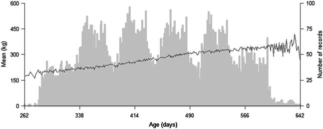
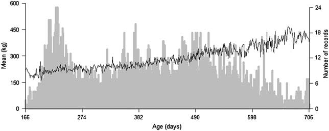
It was observed that body weights increased with age in Nellore and MA young bulls and the distribution of records over ages varied between the two genetic groups (Figures 1 and 2). Approximately 85% and 56% of the records were between 300 and 550 days in Nellore and MA, respectively. This interval contains target ages considered for post-weaning selection (365, 450 and 550 days) in Brazil and represents 66% and 46% of the total intervals in Nellore and MA young bulls, respectively.
Number of records (bars) and mean body weight (black line) according to age for Nellore young bulls in performance tests.

Number of records (bars) and mean body weight (black line) according to age for MA young bulls in performance tests.

Evaluation of fixed-effect model
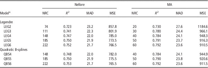
According to the R 2, MAD and MSE criteria, for a given type of polynomial model, the models that used more parameters were the best for the two groups (Table 1). These criteria did not penalise the models for the number of parameters; thus, they favoured the more complex models. When different types of polynomials using the same number of parameters were compared, no difference was detected for the R 2 and MAD criteria. However, in comparisons that considered the MSE, the QBS6 model, which presented the same number of parameters as LEG6, was the best to fit for the Nellore breed. Considering the MA genetic group, the MSE criteria exhibited the lowest values for LEG6.
NRC, coefficient of determination (R 2), MAD (kg) and MSE (kg2) according to the type and order of polynomial to model fixed average growth trajectories of Nellore and MA young bulls in performance tests

NRC=number of regression coefficients; MAD=mean absolute deviation; MSE=mean square error.
a LEGX represents Legendre polynomials with order X-1 and QBSY represents quadratic B-splines with Y-2 intervals.
The Legendre polynomials provided a better fit for the data than the quadratic B-splines only when higher orders were used. In the case of the Legendre polynomials, for which the most suitable model was also LEG6, higher orders may have been necessary because of the unsuitability of the model for modelling the cyclical pattern in the data that is characteristic of growth traits that are subject to seasonal and climatic effects (Arango et al., Reference Arango, Cundiff and Van Vleck2004). According to Kirkpatrick et al. (Reference Kirkpatrick, Hill and Thompson1994) and Meyer (Reference Meyer1998), Legendre polynomials of a high degree must be used to model growth curves, and thus a large number of parameters should be estimated. High-degree polynomials are also associated with numerical problems and have highly demanding computational requirements. The computational requirements can be reduced using B-spline functions, which can improve convergence and reduce computing costs (Bohmanova et al., Reference Bohmanova, Misztal and Bertrand2005). Regardless of the type of polynomial, the models that use more parameters exhibited the best fit for the two genetic groups according to the R 2, MAD and MSE criteria, whereas LEG2 presented the poorest fit (Table 1).
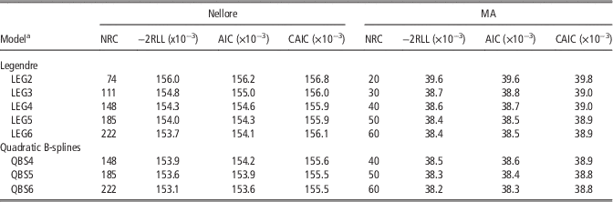
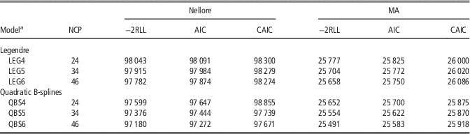
For the same type of polynomial, the –2RLL and AIC criteria demonstrated that LEG6 and QBS6 provided the best fit for the Nellore data. LEG5 and LEG6 fit the data equally well, and QBS6 provided the best fit of the quadratic B-splines for the MA data (Table 2). The CAIC, among the criteria used, imposed the greatest penalty with an increasing number of parameters (Bozdogan, Reference Bozdogan1987 and Wolfinger, Reference Wolfinger1993). Comparing the same type of polynomial, this criterion identified LEG4 and LEG5 as the most suitable models for the Nellore and MA groups, respectively. With respect to the comparisons of the quadratic B-splines polynomials, QBS5 exhibited the best fit for both genetic groups (Table 2).
NRC, values of the restricted likelihood function (–2RLL), AIC and CAIC according to the type and order of polynomial to model fixed average growth trajectories of Nellore and MA young bulls in performance tests

NRC=number of regression coefficients; AIC=Akaike information criteria; CAIC=consistent Akaike information criterion.
aLEGX represents Legendre polynomials with order X-1 and QBSY represents quadratic B-splines with Y-2 intervals.
Considering the –2RLL, AIC and CAIC criteria for general comparisons involving all of the models assessed, the quadratic B-spline polynomials were the best-fitting polynomials. –2RLL and AIC identified QBS6 as the model that best fit the growth data, and CAIC indicated that QBS5 and QBS6 fit the data for the two genetic groups (Table 2). A detailed analysis of the average growth trajectories indicated that the weights estimated by LEG6 were lower until 291 days of age (1.8 kg on average) and greater after an age of 615 days (3.2 kg on average) compared with the weights estimated by QBS6 for the Nellore breed. During the interval from 292 until 614 days, the mean of the differences among the weights estimated by the two models was nearly zero. However, the weights estimated by LEG6 for the Nellore young bulls did not reflect the expected body weight at the final extremity of the age interval.
The weight predicted by LEG6 oscillated sharply at the final extremity of the age interval considered for the two groups (results not shown). Meyer (Reference Meyer1999) and Arango et al. (Reference Arango, Cundiff and Van Vleck2004) emphasised on the difficulties in the application of Legendre polynomials to cattle growth data, particularly because of the greater emphasis that they place on observations at the extremes of the growth curve. To overcome this problem, Meyer (Reference Meyer2005) suggested using B-spline functions, which are curves that are constructed from lower-degree polynomial segments joined at points called knots. Furthermore, B-spline functions are capable of improving the adjustment at the extremes of the age interval because they fit each part of the trajectory according to the number of intervals established.
The QBS6 model described the average growth trajectory of the Nellore and MA young bulls more smoothly and consistently, particularly at the extremes of the age interval. Therefore, this model was considered the most suitable because it exhibited a biological performance closer to that expected for the average growth trajectory (Figures 1 and 2). If Legendre polynomials were used, a better fit could be achieved by using higher-order polynomials. Using high-order Legendre polynomials (quintic, in this case) could have caused problems of biological interpretation of the curve shape, as discussed previously. There is no need to use B-splines with high-order coefficients, and there is better local control (Meyer, Reference Meyer2005) because a set of few functions is considered for each interval, whereas the Legendre polynomial fit one equation with many regression coefficients throughout the range of the independent variable (age).
Fixed and random regression models
Considering models with the same number of covariance parameters, performing random regression with quadratic B-splines to model fixed and random effects provided a better fit for the data compared with Legendre polynomials (Table 3). These results are in agreement with those presented by Meyer (Reference Meyer2005) for the weight of Angus cattle from birth to 820 days. However, Baldi et al. (Reference Baldi, Alencar and Albuquerque2010b) and Boligon et al. (Reference Boligon, Mercadante, Lôbo, Baldi and Albuquerque2012) found that Legendre polynomials performed better than linear, quadratic and cubic B-splines to fit Canchim and Nellore weight data from birth to adult age. According to Meyer (Reference Meyer2005), the lower degrees of B-splines in the individual segments and the local rather than global influence of individual observations partially explain the better fit of B-splines. The age intervals and distribution of records over the range of ages can also be important aspects of data fitting, and thus these factors may affect the type of polynomial that should be used. In addition to the wider range of ages, the distribution of weight records in the data set of Baldi et al. (Reference Baldi, Alencar and Albuquerque2010b) and Boligon et al. (Reference Boligon, Mercadante, Lôbo, Baldi and Albuquerque2012) was less stable than the distributions of records in the data sets of Meyer (Reference Meyer2005) and the present data sets. These distributions might be an additional factor to consider before choosing the type of polynomial to be used in genetic evaluations.
NCP, values of the restricted likelihood function (–2RLL), AIC and CAIC according to the type and order of polynomial to model fixed average growth trajectories and random additive genetic and permanent environmental effects of Nellore and MA young bulls in performance tests

NCP=number of covariance parameters; AIC=Akaike information criteria; CAIC=consistent Akaike information criterion.
aLEGX represents Legendre polynomials with order X-1 to model fixed average growth trajectory and random additive genetic and permanent environmental effects and QBSY represents quadratic B-splines with Y-2 intervals to model the same effects.
The modelling of the fixed average growth trajectory and random additive genetic and permanent environmental effects by quadratic B-splines with three to four regular intervals (QBS5 and QBS6) provided a better fit with the weight data of Nellore and MA bulls submitted to performance tests than other models. Normally, a better fit can be achieved by increasing the number of intervals (Meyer, Reference Meyer2005; Baldi et al., Reference Baldi, Alencar and Albuquerque2010b; Boligon et al., Reference Boligon, Mercadante, Lôbo, Baldi and Albuquerque2012) because each quadratic B-spline function will be responsible for fitting a smaller interval. However, the minimum and mean individual numbers of the records may limit the slicing of an age interval. In random regression models, breeding values for growth are predicted over the age interval, but predictions for animals with few or poorly distributed records are strongly dependent on the animal’s relatives’ records. The minimum of three (MA) and four (Nellore) records and the mean of 4.5 (MA) and 4.8 (Nellore) records per animal might be sufficient to evaluate the current statistical models and to apply them for genetic evaluation of young bulls in performance tests.
The estimates of additive genetic and phenotypic variances for the growth of Nellore and MA young bulls increased over the age interval. The estimates of permanent environmental and residual variances also increased over the age interval for the MA group, but they were constant for the Nellore animals. The additive genetic, permanent environmental, residual and phenotypic variances of weight in performance tests of Nellore and MA young bulls estimated by different Legendre models (LEG4, LE5 and LEG6) were very similar. Considering the Nellore data, the variance estimates were also similar for different quadratic B-spline models. The estimates of additive genetic and phenotypic variances obtained with the QBS6 model were lower than the estimates from the QBS4 and QBS5 models for MA young bulls (results not shown). The pattern of differences in variances were the same as reported for heritability below (Figure 3).
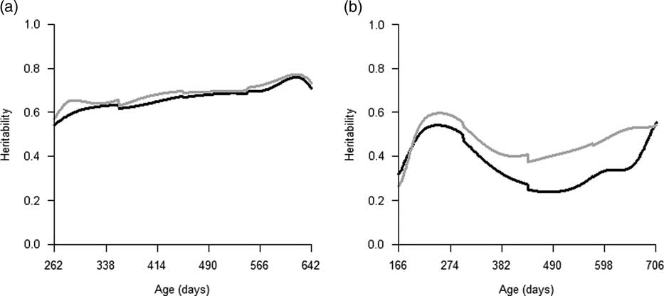
Estimates of heritability for body weight of Nellore (a) and MA (b) young bulls in performance tests with quintic Legendre (grey line) and quadratic B-splines (black line) polynomials with four intervals to model fixed average growth trajectory and random additive genetic and permanent environmental effects.

The estimates of the variances and heritabilities for the weight of Nellore young bulls in random regression models with quintic Legendre (LEG6) or quadratic B-spline (QBS6) polynomials were similar over the age interval (Figure 3a). The increase in heritability and the constant permanent environmental and residual variances indicate that the genetic differences among animals become more evident with age and that selection responses tend to be greater for weight at the end of the performance test for the Nellore group than for weight at other ages.
The estimates of heritability by random regression analysis of the Nellore weights obtained by Albuquerque and Meyer (Reference Albuquerque and Meyer2001) also tended to increase from weaning to 550 days. However, the estimates of permanent environmental and residual variances obtained by Albuquerque and Meyer (Reference Albuquerque and Meyer2001) were not constant. The young bulls in performance tests were kept in the same contemporary group over the total testing period, and changes in the general management were considered minimum. In general, commercial producers tend to change the type of management over time, such as by introducing nutritional supplementation. It is known that minimising changes in the environment is critical for estimating additive genetic variance and to select sires and dams for breeding.
The estimates of additive genetic variance for the weight of MA young bulls using LEG6 and QBS6 tended to increase from the beginning of the age interval to 250 days and to decrease from 250 to 380 days of age. After 380 days of age, the additive variance increased with age, and additive genetic variances in the quadratic B-spline model (QBS6) were lower than the variances in the quintic Legendre (LEG6) model. Baldi et al. (Reference Baldi, Alencar and Albuquerque2010b) found important maternal effects on the weight of Canchim beef cattle until 250 days of age; in the present study, these effects might have been confounded with direct additive genetic effects. However, it was not possible to model maternal effects in the present study because the ratio of young bulls to cow was 1.6 and there were no growth records for cows. A similar constraint was observed by Riley et al. (Reference Riley, Coleman, Chase, Olson and Hammond2007) with growth data of Brahman calves maintained in feedlot during 170 days after weaning. Riley et al. (Reference Riley, Coleman, Chase, Olson and Hammond2007) did not include maternal effects to model body weight of animals and reported inflated estimates of variances because of maternal effects.
Owing to changes in the variances, the estimates of heritabilities for the growth of MA young bulls in performance test (Figure 3b) rapidly increased from the beginning of the age interval to 250 days and decreased from 250 to 440 days of age. After this point, the estimates of heritabilities increased. The estimates of heritability obtained with the quintic Legendre (LEG6) model were markedly greater than the estimates from quadratic B-splines using four intervals (QBS6) after 380 days of age. At the end of the age intervals, the estimates of the heritability obtained with LEG6 and QBS6 became more similar because of the sudden increase in the estimates of heritabilities in the latter model. The estimates of genetic parameters for post-weaning body weight presented in this paper were obtained with data from 884 young bulls sired by 50 Charolais bulls. Of these Charolais bulls, 30 were unrelated or had missing parents. These bulls represented a broad sampling of bloodlines and included prominent bulls of the Charolais breed at that time. Riley et al. (Reference Riley, Coleman, Chase, Olson and Hammond2007) obtained estimates of genetic parameters with data on 724 steers and heifers from a progeny test on 27 Brahman bulls in the United States of America. Despite the small size of MA data (and Brahman data from Riley et al., Reference Riley, Coleman, Chase, Olson and Hammond2007), these results were obtained from a representative sample of MA young bull population and support selection for body weight in the whole population.
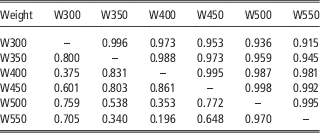
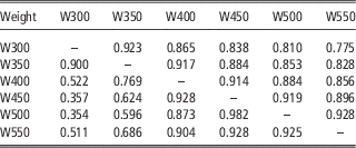
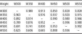
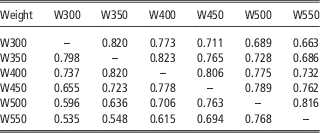
The genetic and phenotypic correlation estimates between weights from the beginning to the end of the performance test over the age interval were moderate to high, and they decreased with increasing distance between weights for the Nellore (Tables 4 and 5) and MA (Tables 6 and 7) bulls. Some unexpected oscillations in the additive genetic (Table 4) and phenotypic (Table 5) correlations among weights in the Nellore young bulls were observed. This situation was also noted by Meyer (Reference Meyer2005) in the analysis of weight from birth to 820 days of age for Australian Angus cattle. According to Meyer (Reference Meyer2005), some effects of joints between pieces of polynomials may have contributed to the oscillations. In general, the results of the present study corroborate those of Albuquerque and Meyer (Reference Albuquerque and Meyer2001) and Boligon et al. (Reference Boligon, Mercadante, Lôbo, Baldi and Albuquerque2012), thereby suggesting that selection for body weight at any age changes the weight at any other age in the same direction. The estimates of correlations among weights were lower in the quadratic B-spline model using four regular intervals than in the quintic Legendre polynomial model. To independently evaluate growth at different points of an animal’s life, the process of obtaining covariables and modelling the fixed and random effects at different points of age intervals using B-splines should be more efficient than Legendre polynomials. One potential consequence is that breeding values for body weight obtained by quadratic B-spline random regression models might be an interesting option to avoid an indirect increase in adult weight being caused by selection for increasing weight at early ages.
Estimates of genetic correlations between body weights of Nellore young bulls from the beginning to the end of age interval of performance tests with quintic Legendre polynomials (above diagonal) to model fixed average growth trajectory and random additive genetic and permanent environmental effects and quadratic B-splines with four regular intervals (below diagonal) to model the same effects

W300, W350, W400, W450, W500 and W550: weight at 300, 350, 400, 450, 500 and 550 days of age, respectively.
Estimates of phenotypic correlations between body weights of Nellore young bulls from the beginning to the end of age interval of performance tests with quintic Legendre polynomials (above diagonal) to model fixed average growth trajectory and random additive genetic and permanent environmental effects and quadratic B-splines with four regular intervals (below diagonal) to model the same effects

W300, W350, W400, W450, W500 and W550: weight at 300, 350, 400, 450, 500 and 550 days of age, respectively.
Estimates of genetic correlations between body weights of MA young bulls from the beginning to the end of age interval of performance tests with quintic Legendre polynomials (above diagonal) to model fixed average growth trajectory and random additive genetic and permanent environmental effects and quadratic B-splines with four regular intervals (below diagonal) to model the same effects

W300, W350, W400, W450, W500 and W550: weight at 300, 350, 400, 450, 500 and 550 days of age, respectively.
Estimates of phenotypic correlations between body weights of MA young bulls from the beginning to the end of age interval of performance tests with quintic Legendre polynomials (above diagonal) to model fixed average growth trajectory and random additive genetic and permanent environmental effects and quadratic B-splines with four regular intervals (below diagonal) to model the same effects

W300, W350, W400, W450, W500 and W550: weight at 300, 350, 400, 450, 500 and 550 days of age, respectively.
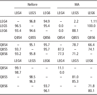
In general, the genetic parameters estimates based on different models were similar, but it is important to evaluate the effects of these small differences on expected progeny differences and the selection process. Because the mean percentages of concordance in the TOP10 animals were greater than 93% in every comparison (Table 8), the number of covariance parameters and the type of polynomial likely did not affect the selection process for body weight in performance tests for the Nellore breed. The results demonstrated the similarity of the estimates of variances and heritabilities based on models with different types of polynomials (Legendre or quadratic B-splines) or different numbers of covariance parameters. However, the differences in variances and heritability estimates for the weight of the MA young bulls in performance tests from different statistical models using different numbers of covariance parameters and types of polynomials appeared to affect the ranking and selection of young bulls (Table 8). The body weight records of the MA young bulls were distributed in a wider interval than the Nellore weights, and a sparse distribution in the last interval might have resulted in poor estimates of fixed and random effects in the MA database. Because of this sparsity, small differences in the adjustment of the fixed average growth trajectory can affect the genetic parameter estimates for the MA genetic group more than those for the Nellore group. This is a common situation that must be addressed in real data sets. In some cases, such constraints limit the model that can be used and its parameterisation.
Means of percentage of concordance in TOP10 Nellore and MA young bulls in each performance test according to expected progeny difference for body weight at 450 (above diagonal) and 550 (below diagonal) days for each pair of statistical modelsFootnote a

a LEGX represents a model with Legendre polynomials of order X-1 to model the fixed effect of average growth trajectory and random additive genetic and permanent environmental effects and QBSY represents a model with quadratic B-spline with Y-2 regular intervals to model the fixed effect of average growth trajectory and random additive genetic and permanent environmental effects.
The percentage of concordance indicates similarity among models and may be used as an additional parameter to compare models. For a real data set, this statistic does not indicate the best model. It only indicates putative differences in the selection process. Despite the difference among –2RLL, AIC and CAIC, genetic evaluation of the body weight of Nellore young bulls submitted to performance tests can be performed using both Legendre and quadratic B-splines and with the most parsimonious models because there is a high concordance in the top-ranked bulls. However, the percentage of concordance in the top-ranked MA bulls also indicated differences among the models. For this genetic group, and most likely all others with poor structures, the statistical evaluation criteria (–2RLL, AIC and CAIC) and biological interpretation should be considered. The results of the present paper suggest that random regression genetic evaluation of MA young bulls in performance tests should be performed with quadratic B-splines of three to four regular intervals.
The quadratic B-spline functions appear to facilitate estimation and simple biological interpretations (Baldi et al., Reference Baldi, Alencar and Albuquerque2010b) and are less susceptible to problems that occur frequently when orthogonal polynomials are used. In the paper, using quadratic B-spline polynomials was satisfactory for the two genetic groups, both for performance tests with the greatest and least number of observations. Generally, greater data dispersion was observed for performance tests with smaller number of observations. However, the data for these performance tests should also be analysed, and more complex models could have difficulties fitting them because of the faults in the data structure. More robust models, such as those with quadratic B-spline polynomials, provided a better fit for the data, even when the data structure was less consistent. Thus, the best fit obtained by the use of quadratic B-spline polynomials was justified by their flexibility in fitting seasonal growth fluctuations in the cattle (Meyer, Reference Meyer2000).
Conclusions
The use of Legendre or quadratic B-spline polynomials was satisfactory for modelling the fixed average growth trajectory and random additive genetic and permanent environmental effects of the Nellore young bulls. It was also possible to choose a parsimonious model for genetic evaluation of the weight of the Nellore young bulls in performance tests. Differences regarding polynomial types and the number of covariance parameters affected the selection process for the MA genetic group, and the quadratic B-splines with three to four equally spaced intervals provided the best fit for the data.
Acknowledgements
The authors thank Humberto de Freitas Tavares (Sucuri Ranch – Provados a Pasto), Maurício Mello de Alencar (Embrapa Cattle – Southeast) and João Paulo Porto (Santa Helena Ranch – Agropecuária Ipameri) for allowing the use of databases for this study. Pró-Reitoria de Pesquisa/Universidade Federal de Minas Gerais funded the translation of the paper, FAPEMIG funded facilities for this research (PPM-00456-11), CNPq funded Fabio Luiz Buranelo Toral (Process 502401/2009-5) and Breno de Oliveira Fragomeni (studentship) and CAPES funded Daiane Cristina Becker Scalez (studentship).