I. INTRODUCTION
Periodic truss structures can be designed to have high specific strength and specific stiffness in combination with other desirable attributes, including high energy absorption capacity Reference Zheng, Zhao and Fan1–Reference Asadpoure, Tootkaboni and Valdevit3 and effective internal heat exchange. Reference Wadley4,Reference Maloney, Fink, Schaedler, Kolodziejska, Jacobsen and Roper5 Most truss topologies, however, exhibit strongly anisotropic mechanical properties: an undesirable characteristic when trusses are used in applications in which the directions of loading are not known a priori. The present study addresses the design of lightweight (low relative density) truss structures that are elastically isotropic and that also exhibit high strength. The designs are based principally on compound trusses comprising two or more elementary cubic trusses that, on their own, are highly anisotropic.
Realizing these and other designs has been made possible by recent advancements in additive manufacturing. For example, polymeric and polymer-derived ceramic trusses have been fabricated using self-propagating photopolymerization. Reference Jacobsen, Barvosa-Carter and Nutt6–Reference Eckel, Zhou, Martin, Jacobsen, Carter and Schaedler8 Very low relative density metallic lattices have been formed by electroplating and etching away a polymeric template. Reference Schaedler, Jacobsen, Torrents, Sorensen, Lian, Greer, Valdevit and Carter9,Reference Torrents, Schaedler, Jacobsen, Carter and Valdevit10 Novel lithography techniques such as direct laser writing and projection micro-stereolithography have been used to fabricate fractal-like trusses composed of self-similar members that span length scales of several orders of magnitude. Reference Meza, Zelhofer, Clarke, Mateos, Kochmann and Greer11,Reference Zheng, Smith, Jackson, Moran, Cui, Chen, Ye, Fang, Rodriguez, Weisgraber and Spadaccini12 Experimental measurements and theoretical analyses have shown that these hierarchical structures exhibit nearly linear scaling of stiffness and strength even at very low relative densities (<1%). Reference Lakes13–Reference Jang, Meza, Greer and Greer15
To achieve linear scaling between mechanical properties and relative density, truss deformation must be dominated by strut stretching. In stretch-dominated trusses, struts are loaded axially in either tension or compression, and thus, the macroscopic truss stiffness is proportional to the extensional strut stiffness. Since extensional stiffness (determined from the cross-sectional area of the struts) scales linearly with relative density, stiffness scales similarly: E ∝ E oρ, where E and E o are the Young’s moduli of the truss and the constituent strut material, respectively, and ρ is the relative density. Analogously, if truss failure is dominated by yielding, the yield stress σy also scales linearly with ρ: σy ∝ σy,oρ, where σy,o is the yield strength of the solid. By contrast, random networks exhibit bend-dominated behavior; that is, rather than changing length, struts bend under an applied load, and thus, truss stiffness and strength are proportional to the bending stiffness and yield strength, respectively. As a result, these properties follow power-law scalings with relative density: E ∝ E oρ2 and σy ∝ σy,oρ1.5. Reference Gibson and Ashby16 To retain favorable scaling (∝ρ) at low relative densities, trusses must be designed to ensure stretch-dominated response.
Truss design can follow one of two broad approaches. In the first, computational algorithms based on finite elements are used for shape and topology optimization. Reference Asadpoure and Valdevit17–Reference Sigmund20 For structural problems, the entire allowable spatial domain is discretized into finite elements; the properties of the elements form the design variables. An optimization problem is formulated from an objective function and a set of constraints, the latter including mechanical equilibrium of the structure and allowable material volume. Using this approach, elastic moduli have been maximized under constraints of elastic isotropy and fixed relative density. Reference Osanov and Guest21,Reference Challis, Roberts and Wilkins22 Moduli were calculated from the response of trial structures to various applied test fields. Gradient-based optimization methods were used to find (local) optima. The moduli of resulting topologies have been shown to approach the Hashin–Shtrikman upper bound. However, in general, the topologies are complex and the structures would be difficult to fabricate, even with current additive manufacturing techniques. An additional drawback of this “top-down” approach is that it rarely yields insights into general design principles with broad application.
The second approach (used here) follows a “bottom-up” path. Notably, elementary truss structures are combined in judicious ways to create trusses in which the positive attributes of the constituent trusses are exploited while their shortcomings are ameliorated. In essence, the topology is fixed at the outset while certain geometric parameters are systematically varied. The resulting design space is much smaller than that in the more general topology optimization approach.
The present designs stem from a recently developed framework of truss taxonomy and classification. Reference Zok, Latture and Begley23 The framework consists of a hierarchy of topological complexity. At the simplest level, elementary cubic trusses are formed by joining the nearest-neighbor points of a cubic space lattice with struts, thereby yielding either simple cubic {SC}, body-centered cubic {BCC}, or face-centered cubic {FCC} truss types. Specific truss designs are denoted {nA} b , where n is the lineal number of unit cells, A is the truss type (SC, BCC, or FCC), and b is the number of directions in which the cells are tiled (1, 2, or 3).
A compound cubic truss is produced by combining two or more elementary cubic trusses onto a common space lattice. When the elementary trusses are combined in pairs, the procedure yields three binary compound truss types, designated {BCC}|{SC}, {FCC}|{SC}, and {FCC}|{BCC}. Specific truss designs are defined (as with elementary trusses) by adding the lineal number n of unit cells and the dimensionality b to the designation. Translations and rotations of the coordinate system that define the second truss in the designated sequence are denoted by appending the truss designation by [u v w] and (θ x θ y θ z ), respectively. When absent, the latter are implied to be zero. More complex trusses are obtained by (i) applying affine deformations to the cubic trusses; (ii) assigning two or more nodes to each point of a space lattice and constructing the truss by placing struts between nearest-neighbor nodal locations; or (iii) constructing a supercell from an assemblage of two or more elementary sub-cells and then duplicating and tiling the supercell. The present study is restricted to elementary and compound cubic trusses.
The principal goal of the study is to identify designs of trusses that (i) are elastically isotropic, (ii) exhibit high specific stiffness, and (iii) have potential for high strength under various loading scenarios, including compression, tension, and shear. Preliminary insights into the design strategy are obtained from examination of the topology of elementary cubic trusses. Because of the alignment of struts along the edges of its unit cell, the {SC} truss is stiff along the body edges but highly compliant in other loading directions, e.g., along the face diagonal or the body diagonal. By contrast, the {BCC} truss is stiff along the body diagonal and compliant in other directions. Footnote a Since the two trusses exhibit high stiffness along different directions, we expect that combining {SC} and {BCC} trusses onto a common space lattice should yield a compound truss with a higher degree of isotropy than those of the constituent elementary trusses. The {FCC} truss is stiffest along the body diagonal and most compliant along the body edge: the ratio of minimum to maximum stiffness being 5/9. Reference Deshpande, Fleck and Ashby24 Although this truss is the most isotropic of the three, we expect that its low stiffness along the body edges might be mediated by the addition of a {SC} truss. Since both {FCC} and {BCC} trusses are stiff along the body diagonal and more compliant along the body edges, a compound truss comprising these two would not be expected to yield improved isotropy.
In a recent study, Gurtner and Durand identified an elastically isotropic truss that exhibits the maximal stiffness for strut-based structures.
Reference Gurtner and Durand25
The truss type has been called, interchangeably, a regular truncated octahedron, a Kelvin cell, or a reinforced BCC.
Reference Pettermann and Hüsing26
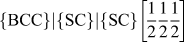
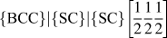
By our classification, it is of the type
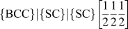
 $\left\{ {{\rm{BCC}}} \right\}\left| {\left\{ {{\rm{SC}}} \right\}} \right|\left\{ {{\rm{SC}}} \right\}\left[ {{1 \over 2}{1 \over 2}{1 \over 2}} \right]$
; that is, it consists of an array of {BCC} and {SC} trusses with coincident nodal locations and an array of {SC} trusses with an origin offset by a distance
 $\left[ {{1 \over 2}{1 \over 2}{1 \over 2}} \right]$
relative to the origin of the first two trusses. In what follows, we present a simpler isotropic compound truss that exhibits the same stiffness and that is more robust in the inelastic (post-buckling) regime of loading.
To provide context for subsequent analyses of buckling failure (the mode that invariably dominates when the relative density is sufficiently low), we find it useful to couch the discussion in terms of three distinct factors governing failure:
-
(i) The average axial strut strain εa relative to the global (applied) strain ε in each of the constituent strut populations;
-
(ii) The strut slenderness ratio l/r, where l is the strut length and r is its radius (assuming circular cross-sections); and
-
(iii) The constraints imposed on the strut ends by adjoining struts, characterized by the effective length factor K in Euler buckling theory.
As we show in due course, the macroscopic failure strain of trusses that fail by buckling is proportional to (ε/εa)(r/Kl)2.
An additional implicit factor in truss failure is the nodal connectivity, Z. All other factors kept constant, high values of Z lead to increased constraints on the strut ends and increased buckling resistance, as manifested in low K. Nodal connectivity is also indirectly related to strut slenderness; that is, if relative density is kept constant, an increase in connectivity must be accompanied by a higher number density of struts which, in turn, must be accommodated by lower strut radius and hence higher slenderness ratio. The preceding two effects act in opposition: the former inhibiting buckling and the latter promoting buckling as Z increases. When Z is sufficiently small (say <12), truss deformation is dominated by strut bending and the average axial strut strains are negligible. Reference Buxton and Clarke27 Instead, deformation is accommodated by changes in strut curvature and failure occurs by mechanisms other than buckling (i.e., yielding or fracture).
The article is laid out in the following way. Truss topologies, finite element (FE) models, and solution methods are described in Sec. II. Elastic properties of the trusses of interest are presented in Sec. III. The axial strut strains and their spatial variations are considered in Sec. IV. Inelastic (buckling) responses are addressed in Sec. V. Effects of truss size, characterized by the number of unit cells in a cubic array of such cells, are also explored.
II. METHODS
A. Topologies, geometry, and models
FE computations were used to ascertain the mechanical properties of, specifically, the: (i) elementary cubic trusses {nSC}3, {nFCC}3, and {nBCC}3, (ii) binary compounds {nFCC}3|{nSC}3 and {nBCC}3|{nSC}3, and (iii) ternary compounds {nFCC}3|{nBCC}3|{nSC}3 and
 ${\left\{ {n{\rm{BCC}}} \right\}^3}|{\left\{ {n{\rm{SC}}} \right\}^3}|{\left\{ {\left( {n - 1} \right){\rm{SC}}} \right\}^3}\left[ {{1 \over 2}{1 \over 2}{1 \over 2}} \right]$
(the latter being the isotropic truss identified by Gurtner and Durand).
Reference Gurtner and Durand25
Here, n was varied from 1 to 11. Structures were discretized using three-dimensional Timoshenko beam elements with circular cross-section. Strut dimensions were selected to yield a relative density of ρ = 0.01. (Other FE simulations, with ρ ranging from 0.001 to 0.05, yielded virtually identical results when normalized by relative density accordingly.) The properties of the parent material were taken to be as follows: Young’s modulus E
o = 200 GPa, shear modulus G
o = 80 GPa, and mass density ρo = 7800 kg/m3. Strut intersections were modeled as rigid joints. In compound trusses, all struts of a specific constituent truss were assigned the same cross-sectional area, dictated by the total volume fraction of the material allocated to that truss type. The proportions of volumes allocated to each constituent truss within the compounds were varied from 0 to 1 in increments of 0.01. Models were processed using the commercial package Abaqus (Version 6.13-EF4, Dassault Systémes, Providence, Rhode Island).
B. Elastic properties
Elastic properties were computed for uniaxial normal loading (compression or tension) along one of the principal directions (denoted 1) and in pure shear (in the 1–2 plane) using Abaqus/Standard. A state of uniaxial compression was obtained by prescribing displacements of lattice points on opposing faces of the model: u = ε1 L at x = L and u = 0 at x = 0, where u is the nodal displacement along the 1-axis, x is the position on the 1-axis, ε1 is the strain in the 1-direction, and L is the length of the truss along the principal directions. Here, lattice points are defined by the space lattice before discretizing struts into beam elements. Rigid body motion of the model was prevented by pinning the lattice point at the origin, i.e., u = v = w = 0 at (0, 0, 0), where v and w are the nodal displacements along the 2- and 3-axes, respectively, and assigning w = 0 for the lattice point at (0, L, 0). Analogously, a state of pure shear was obtained by prescribing nodal displacements on the 1- and 2-faces: v = ε12 L/2 at x = L, v = −ε12 L/2 at x = 0, u = ε21 L/2 at y = L, and u = −ε21 L/2 at y = 0. Rigid body motion was constrained in shear by imposing w = 0 at (0, 0, 0) and (0, L, L). No additional constraints were imposed in either load state when calculating elastic properties. These boundary conditions best simulate deformation of a finite truss and were chosen to study effects of truss size on elastic properties. In all cases, the global engineering strains were 0.02, i.e., ε1 = 0.02 for uniaxial compression and γ12 = ε12 + ε21 = 0.02 for pure shear. From the corresponding computed reaction forces, the Young’s modulus, E 1, shear modulus, G 12, and Poisson ratio, ν12, were computed.
The degree of elastic anisotropy was ascertained from the variation in axial stiffness with loading direction. The stiffness along a vector 〈ijk〉 is related to the elastic constants via Reference Nye28
 $${1 \over {{E_{ijk}}}} = {1 \over {{E_1}}} - 2\left( {{\alpha ^2}{\beta ^2} + {\beta ^2}{\gamma ^2} + {\alpha ^2}{\gamma ^2}} \right)\left( {{1 \over {{E_1}}} - {1 \over {2{G_{12}}}} - {{{\nu _{12}}} \over {{E_1}}}} \right)\quad ,$$
where α, β, and γ are the direction cosines between 〈ijk〉 and the principal coordinate axes. The results are presented as polar plots of E ijk .
Based on symmetries in loading and truss topologies, struts are grouped in the following way. In {FCC}, type I struts are aligned along [110] and
 $\left[ {1\bar{1}0} \right]$
directions, type II struts are aligned along [101] and
 $\left[ {10\bar{1}} \right]$
directions, and type III struts aligned along [011] and
 $\left[ {01\bar{1}} \right]$
. Type I and II struts are oriented at 45° to the compression direction, whereas type III struts are perpendicular to the compression direction. Additionally, type I and II struts are loaded in opposite directions under an applied shear strain, γ12. In {SC}, type IV struts comprise [100] (parallel to the compression direction) and type V comprise [010] and [001]. In {BCC}, type VI struts comprise [111] and
 $\left[ {\bar{1}11} \right]$
and type VII struts comprise
 $\left[ {1\bar{1}1} \right]$
and
 $\left[ {11\bar{1}} \right]$
. The latter two are loaded in opposite directions under an applied shear strain.
C. Strut strains
Axial strut strains, εa, resulting from the application of either uniaxial loading, ε1, or pure shear, γ12, in an infinite truss (n = ∞) were calculated using the direct stiffness method. For this purpose, a single unit cell was modeled using periodic boundary conditions. The boundary conditions were adapted from a method outlined by Wallash and Gibson whereby nodal displacements on opposing faces of the model are linked via linear multipoint constraints. Reference Wallach and Gibson29 This method assumes that faces remain planar and does not consider rotational degrees of freedom. The omission of the latter is valid in stretch-dominated trusses provided struts have not buckled (in which case, nodal rotations are negligible). In their analysis, Wallash and Gibson reported errors due to the neglect of bending moments in reaction forces of approximately 1.4%. We expect to get similar errors in the present analysis. The cross-sectional area of struts shared between adjacent cells was properly adjusted to avoid over counting. Results are presented for each unique strut population for a given type of loading.
To ascertain the strain amplifications due to external boundaries, axial strut strains resulting from the application of uniaxial compression were also calculated for struts in finite trusses. The results were sorted in two ways: (i) by strut type (I–VII) and (ii) by strut location, characterized by the distance δ from the strut centroid to the nearest external free boundary.
D. Inelastic response
The inelastic responses for uniaxial compression, pure shear, and uniaxial tension were computed for finite trusses using Abaqus/Explicit. Boundary conditions were analogous to those used for the elastic simulations, except that nodal velocities (rather than displacements) were prescribed, e.g., velocity,
 $\dot{x} = {{{\rm{d}}x} \over {{\rm{d}}t}} = \dot{\varepsilon }L$
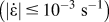
at x = L for uniaxial compression. Velocities were selected to yield quasi-static strain rates
 $\left( {\left| {\dot{\varepsilon }} \right| \le {{10}^{ - 3}}\;{{\rm{s}}^{ - 1}}} \right)$
. The resulting ratio of the kinetic to potential energy was less than 10−3 for all time steps in each simulation, confirming quasi-static loading. The equations of motion were integrated using explicit central differences with fixed timestep until reaching a global strain of 2%. To smoothly traverse bifurcation (buckling) phenomena in the solution path, imperfections consistent with the first three buckling modes were superimposed according to the geometric sequence:
 $$\Delta \bar{x} = n\sum\limits_{i = 1}^3 {B{{\left( r \right)}^{i - 1}}{{\bar{\phi }}_i}} \quad ,$$
where
 $\Delta \bar{x}$
is the resultant vector of nodal displacements applied to the original nodal coordinates, n is the lineal number of unit cells, B is the amplitude applied to the first buckling mode, r is the ratio of geometric progression, and
 $\bar{\phi }$
contains the set of nodal displacements of the ith mode shape normalized such that the maximum displacement is equal to 1.0. Here, B was taken to be 0.001 and r was 1/2.
Imperfections of this type do not affect the ultimate truss strength. In the trusses of present interest, failure is governed by elastic buckling of families of struts that are, on average, equally strained. Here, the macroscopic truss strength is dictated by the volume-averaged strut stress once all struts have buckled. Because the stress needed for continued strut buckling is constant (i.e., the strut response is effectively elastic, perfectly plastic), a premature buckling event caused by a structural imperfection does not significantly affect the ultimate strength.
Interestingly, without imperfections, the buckled solution can still be found; numerical integration of the equations of motion introduces errors into nodal displacements that serve the same purpose as artificial imperfections. But, since the integration errors and the resulting imperfections are small, buckling causes intense high frequency oscillations. Seeding structural imperfections dramatically reduces these effects. Even with structural imperfections, weak high frequency oscillations are still obtained. As a result, a small amount of damping was introduced in the form of linear bulk viscosity. The viscosity generates a pressure,
 $p = \zeta {\rho _{\rm{o}}}{c_{\rm{d}}}{l_{\rm{e}}}{\dot{\varepsilon }_{{\rm{vol}}}}$
, where ζ is a damping coefficient, ρo is the material density, c
d is the dilatational wave speed, l
e is the length of the element, and
 ${\dot{\varepsilon }_{{\rm{vol}}}}$
is the volumetric strain rate. For all simulations, ζ = 0.06. Linear bulk viscosity of this form is included by default in Abaqus/Explicit.
E. Buckling strengths
The preceding results were interpreted in the context of Euler buckling theory. For reference, the critical load P c for strut buckling is given by P c = π2 EI/(Kl)2, where E is the Young’s modulus; I is the second moment of area of the strut cross section; l is its length; and K is the nondimensional effective-length factor, dictated by the degree of constraint at the strut ends. For example, if transverse displacements and rotations were fully constrained at both ends, K = 1/2; this condition yields the highest buckling load. By contrast, if both strut ends were pin-jointed and displacements of the endpoints were only allowed along the strut axis, K = 1. Yet higher values of K would be obtained as the number of degrees of freedom of the strut ends is increased.
In the current study, values of K for each strut population were inferred from the average axial strut strain
 ${\bar{\varepsilon }_{\rm{a}}}$
at the point of buckling of the respective strut population, via
 $K = \pi r{\rm{/}}2l\sqrt {{{\bar{\varepsilon }}_{\rm{a}}}}$
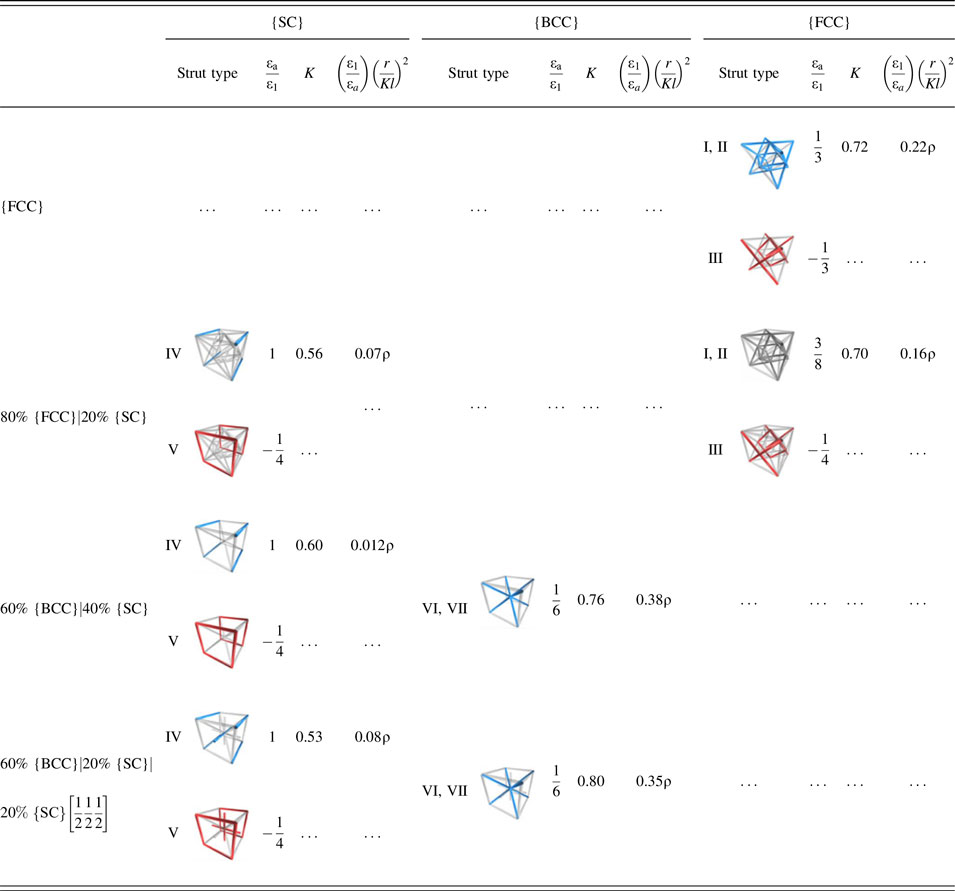
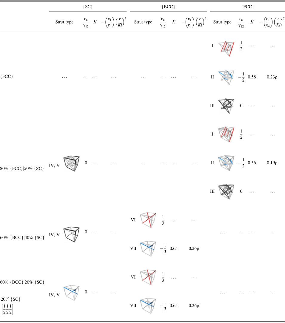
. The results were further combined to compute three buckling metrics, defined by βc = (ε1/εa)(r/Kl)2 in compression, βt = −(ε1/εa)(r/Kl)2 in tension, and βs = −(γ12/εa)(r/Kl)2 in shear, for each strut population. The values of the metrics provide quantitative measures of the resistance of the struts to buckling for each truss type, taking into account strut slenderness (summarized in Table SI), axial strut strain (Tables I–III), and constraints at the nodes, the latter governed by the number and nature of struts passing through the nodes.
Strut strains, buckling metrics, and truss strengths for compressive loading.
III. ELASTIC PROPERTIES
A. Elementary cubic trusses
The three elementary cubic trusses exhibit a wide range of elastic properties and anisotropy. (Polar plots of their axial stiffness for large n are shown in Fig. S1.) For reference, the maximal stiffness for strut-based isotropic trusses is E/E oρ = 1/6. Reference Gurtner and Durand25 Both the {SC} and {BCC} trusses are mechanisms; they exhibit high stiffness only along directions parallel to strut directions and are highly compliant in other directions. Specifically, the maximum stiffness of {SC} is E/E oρ = 1/3, along 〈100〉-type directions, whereas the maximum stiffness of {BCC} is E/E oρ = 1/9, along 〈111〉-type directions. On their own, these trusses do not make useful structures. Among the elementary trusses, the {FCC} truss is closest to isotropic. Its stiffness is E/E oρ = 1/9 and 1/5 along 〈100〉- and 〈111〉-type directions, respectively.
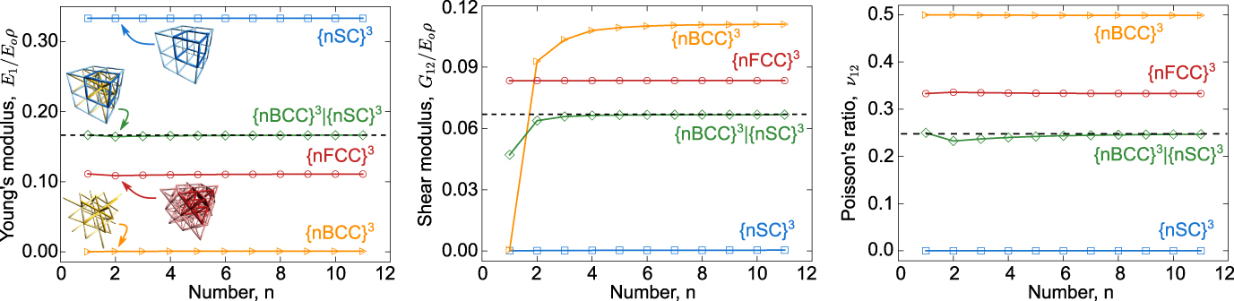
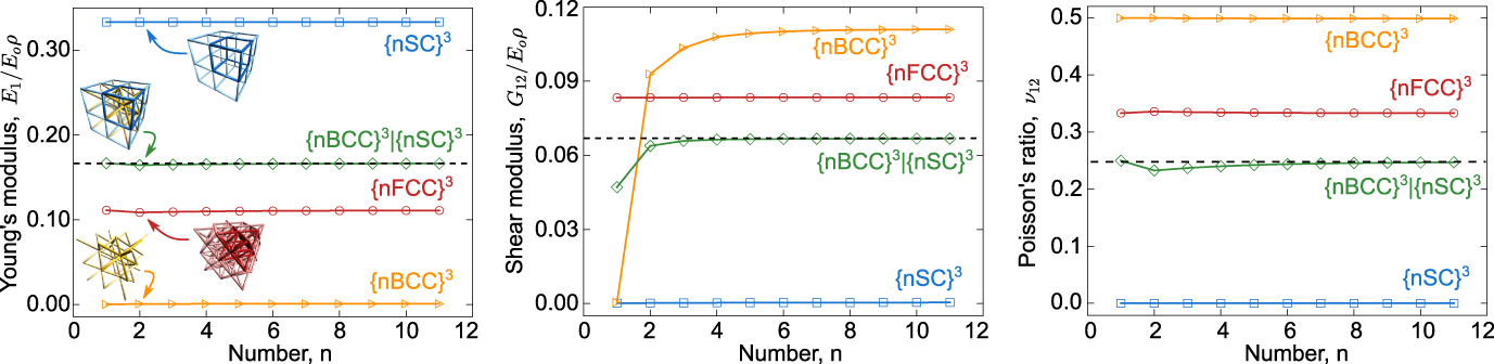
The elastic properties of the elementary cubic trusses are essentially independent of n (Fig. 1). One exception is the shear modulus of the {BCC} truss; the average nodal connectivity decreases from 8 when n = ∞ to 1.7 when n = 1. Consequently, its shear modulus goes to 0 as n goes to 1.
Elastic properties of cubic truss structures with finite size normalized by Young’s modulus of the parent material and relative density of the truss. The Young’s modulus of the {nBCC}3 truss and the shear modulus of the {nSC}3 truss are 0.0006 and 0.0002, respectively: both close to but not identically zero, a consequence of rigid connections at the nodes.
B. Binary compound trusses
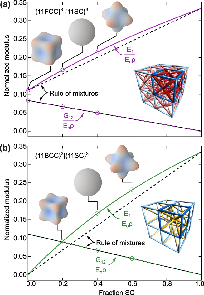
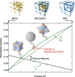
Stiff isotropic trusses are obtained for select combinations of elementary trusses. Variations in the elastic constants with volume fraction of the constituent trusses in the binary compounds are plotted in Fig. 2 for n = 11. Also shown are the values based on rule-of-mixtures predictions. The latter predictions tacitly assume that the constituent trusses behave independently of each other, i.e., without mechanical coupling. Representative polar plots of the axial stiffness are also included as insets. Videos showing the evolution of axial stiffness and elastic moduli are provided in the Supplementary Material (VIDS. S1 and S2). Key observations follow.
Young’s and shear moduli for binary trusses comprising {SC} and either (a) {FCC} or (b) {BCC} trusses. Insets are polar plots of axial stiffness. (See also VIDS. S1 and S2 in the Supplementary Material.)
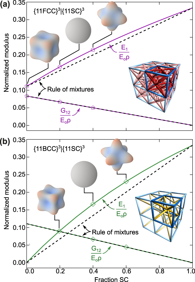
The compound trusses 80% {FCC}|20% {SC} and 60% {BCC}|40% {SC} are isotropic. Footnote b Their Young’s moduli are slightly higher than rule of mixtures prediction. This is because type V struts, which are perpendicular to the loading axis and stress-free in the elementary structure, are placed into tension in the compound truss, thereby constraining the lateral node displacements. In shear, the {SC} struts (type IV and V) are not loaded and do not contribute to the shear modulus. Thus, the shear modulus is well represented by the rule of mixtures, in this case given by the product of the volume fraction and modulus of the constituent {FCC} or {BCC} sub-trusses.
Here, again the elastic properties are insensitive to n. Variations of the elastic constants with n for the isotropic 60% {BCC}|40% {SC} truss are shown in Fig. 1. Reported properties of isotropic trusses that are maximally stiff are also shown: E 1/E oρ = 1/9, G 12/E oρ = 1/15, and ν12 = 1/4. Reference Gurtner and Durand25 Young’s modulus and Poisson’s ratio of the compound truss are virtually independent of n and are equivalent to those of the predicted maximal value. A reduction in shear modulus for the compound truss is observed below n = 3. Similar to the response of {BCC} in shear, the reduction of average nodal connectivity that accompanies the reduction in n leads to a more compliant truss. Variations in the elastic properties of the isotropic {FCC}|{SC} truss are not shown; by design, its properties are identical to those of the {BCC}|{SC} truss (at least at large n).
C. Ternary compound trusses
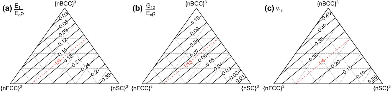
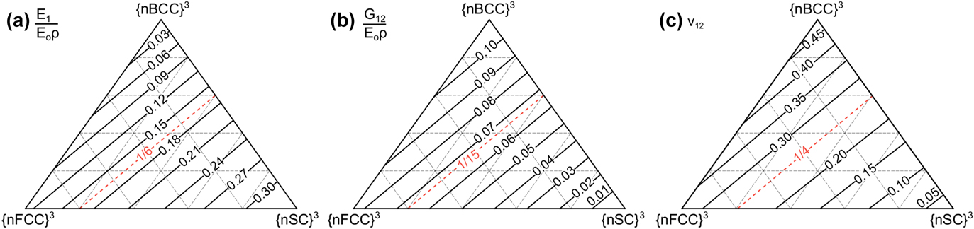
Stiff isotropic trusses are also obtained with certain ternary {FCC}|{BCC}|{SC} compound trusses. Their elastic properties are shown in Fig. 3. Each property is presented within a Gibbs triangle; each corner represents one of the three elementary trusses, each edge corresponds to one of the three binaries, and the interior regions correspond to the ternaries. Contours show compositions at which the properties are of constant value. Contours highlighting compositions that exhibit elastic properties of isotropic maximally stiff trusses are also shown. The latter compositions follow straight lines joining the two isotropic binary trusses, namely 80% {FCC}|20% {SC} and 60% {BCC}|40% {SC}. All trusses along this line are isotropic and exhibit the highest possible stiffness. Notably, absent from the latter are binary combinations of {FCC} and {BCC}. As noted previously, since each of these trusses on its own exhibits high compliance along the body edges, combinations of the two do not ameliorate their inherent anisotropy.
(a) Young’s modulus, (b) shear modulus, and (c) Poisson’s ratio for ternary combinations of {SC}, {FCC}, and {BCC} trusses.
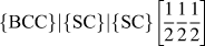
Gurtner and Durand identified another maximally stiff isotropic ternary truss of the type
 $\left\{ {{\rm{BCC}}} \right\}|\left\{ {{\rm{SC}}} \right\}|\left\{ {{\rm{SC}}} \right\}\left[ {{1 \over 2}{1 \over 2}{1 \over 2}} \right]$
.
Reference Gurtner and Durand25
In their treatment, the cross-sectional areas of struts in the two {SC} trusses were taken to be equal to one another. The ratio of cross-sectional areas, s, of the {BCC} struts and the {SC} struts for maximal isotropic stiffness is
 ${s_{{\rm{BCC}}}}{\rm{/}}{s_{{\rm{sc}}}} = 3\sqrt 3 {\rm{/}}4$
. This equates to approximately 60% of {BCC} and 20% of each of the two {SC} trusses. As we show below, the analogous binary truss (with equivalent elastic properties) is more robust in the post-buckling domain.
IV. STRUT STRAINS
A. Infinite trusses
As a prelude to the nonlinear buckling responses of the trusses of interest, we present results for the axial strut strains when the trusses are loaded elastically in compression, in tension, and in shear. The trusses of interest are the (anisotropic) {FCC} truss, the isotropic binary trusses {FCC}|{SC} and {BCC}|{SC}, and the isotropic ternary truss
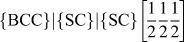 $\left\{ {{\rm{BCC}}} \right\}|\left\{ {{\rm{SC}}} \right\}|\left\{ {{\rm{SC}}} \right\}\left[ {{1 \over 2}{1 \over 2}{1 \over 2}} \right]$
. The axial strut strains, εa, normalized by the respective applied strains, ε1 or γ12, for infinite trusses are summarized in Tables I–III.
Strut strains, buckling metrics, and truss strengths for tensile loading.
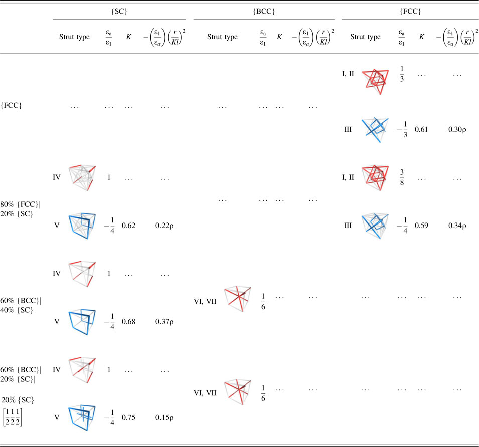
When the {FCC} truss is loaded in compression, the axial strain in type I and II struts (inclined at 45° to the loading direction) is εa/ε1 = 1/3 while that in type III struts (perpendicular to the loading direction) is εa/ε1 = −1/3. The axial strains in the {FCC} struts within the isotropic {FCC}|{SC} truss differ slightly: εa/ε1 = 3/8 for types I and II and εa/ε1 = −1/4 for type III. The differences arise because of the constraints imposed by the {SC} struts. The strains in type IV and V struts within the binary truss are εa/ε1 = 1 and −1/4, respectively. (The ratio of the latter two strains emerges naturally from the fact that the Poisson’s ratio for the isotropic maximally stiff truss is 1/4. Reference Gurtner and Durand25 ) The difference in the axial strains in the compressed struts in the elementary and compound trusses (1/3 versus 3/8) suggests a slightly higher propensity for strut buckling in the compound truss at a prescribed macroscopic strain. The results of strut strains for tensile loading are the same, except for a sign change.
For shear loading, the axial strut strains in the {FCC} truss are εa/γ12 = 1/2, −1/2, and 0 in type I, II, and III struts, respectively. The same results are obtained for the {FCC} struts within the binary {FCC}|{SC} truss. Here, the {SC} struts experience no axial strain and, therefore, have no effect on the elastic response of the {FCC} sub-truss (apart from the reduction in the diameter of the {FCC} struts, to maintain constant relative density).
When compound isotropic trusses (both binary and ternary) containing {BCC} struts are loaded in compression, all such struts experience the same axial strain: εa/ε1 = 1/6. (On its own, the elementary {BCC} truss is entirely bend-dominated and thus the struts experience negligible axial strain.) Again, the strains in type IV and V struts within the {SC} truss are εa/ε1 = 1 and −1/4. For shear loading, the strains in the {BCC} sub-truss are εa/γ12 = 1/3 and −1/3 while the constituent {SC} struts experience no axial strain.
B. Boundary effects in finite trusses
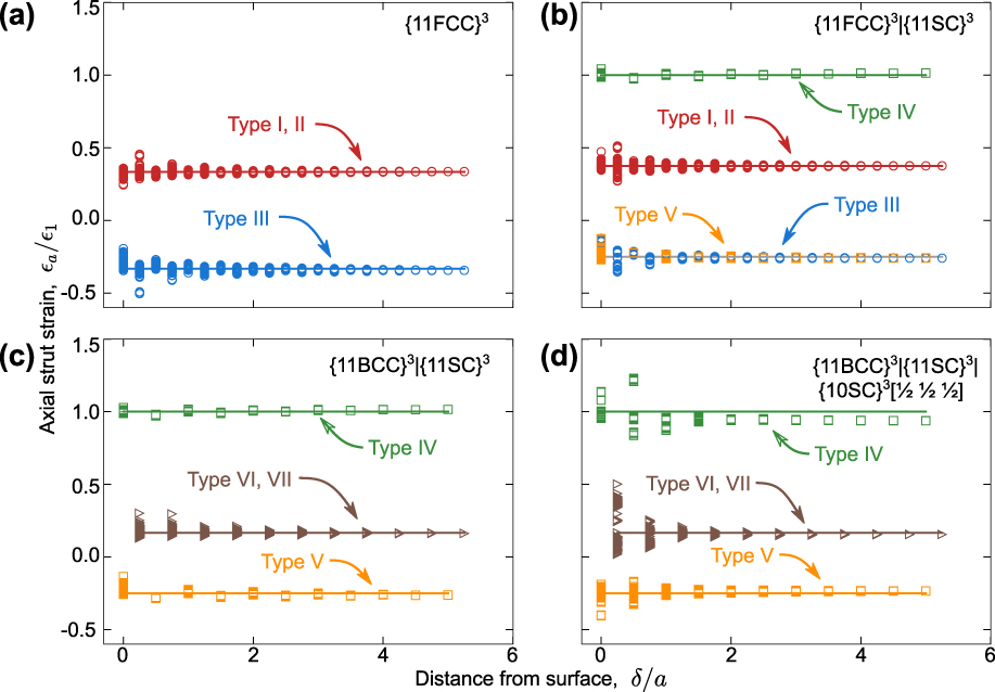
Strut strains differ in near-boundary regions because of local differences in connectivity and constraint. Effects of boundaries on strut strains for compressive loading of trusses with n = 11 are shown in Fig. 4. Strains are plotted against the normalized distance δ/a from the centroid of a strut to the nearest external free boundary. Data points are labeled by truss type and solid lines indicate predicted strains in infinite trusses. In all cases, some of the near-boundary struts experience a strain that is significantly greater or less than the average value.
Variations in axial strut strains with distance from the nearest external free boundary.
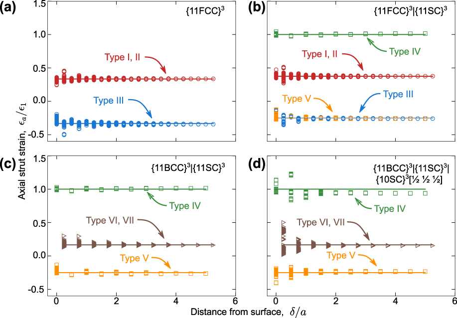
The maximum strain amplification in type I and II struts in the {FCC} truss is about 50%. εa/ε1 is as high as 1/2 for type I and II struts.
 ${\left({{\rm{1}} \over 2}}$
-
 ${{{1 \over 3}} \right)}/{\left({1 \over 3}} \right)$
*100 = 50%. The amplification persists over distances of about δ/a = 2 into the truss interior. Type III struts in this truss experience a maximum (tensile) strain of εa/ε1 = −1/2: 50% greater than the average value for that strut population. The most heavily strained struts are the ones that intersect the truss edges (see VID. S3 in the Supplementary Material). In the two binary trusses, the strain amplification within {SC} struts is negligible. By contrast, {BCC} and {FCC} struts in the two binary trusses experience strain amplifications as high as 80% and 35%, respectively. Even higher amplifications are obtained in the near-surface {BCC} struts in the ternary truss. In these cases, the effects also persist to depths of δ/a ≈ 2.
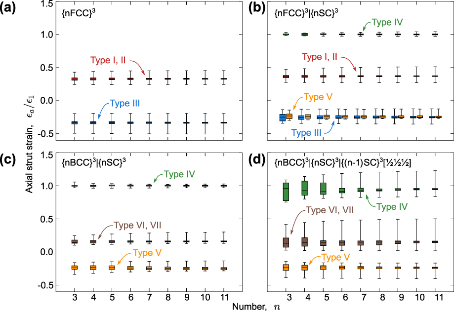
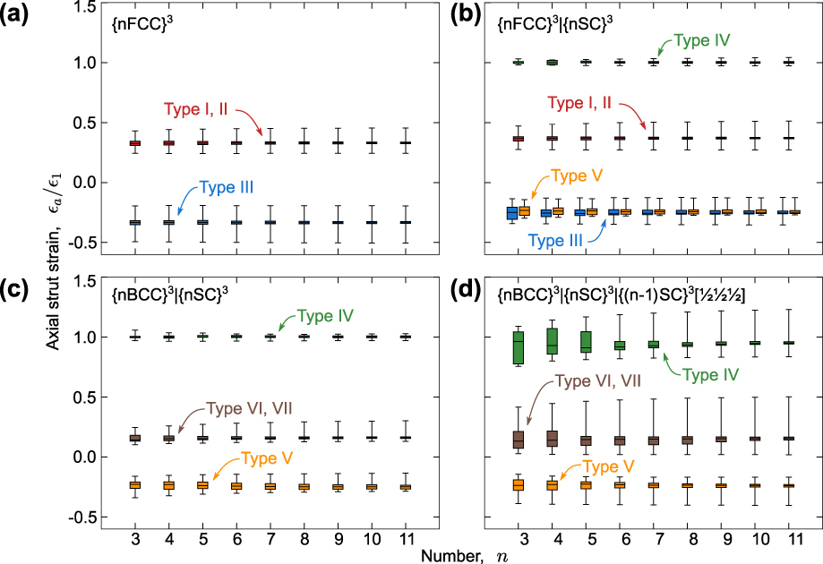
The magnitude of strain amplification does not change appreciably with truss size. Distributions in axial strut strains for n = 2 − 11 are shown in Fig. 5. Within a given strut type, the minimum and maximum strains are virtually independent of n. The middle two quartiles of data shrink as n increases because an increasing fraction of struts is located away from external boundaries. Strain amplifications for struts of the same type can be highly dependent on truss type. Type III struts of the elementary {FCC} truss [Fig. 5(a)] on average experience greater strain amplification than that for struts in the compound truss [Fig. 5(b)]. The most significant changes between corresponding struts of different trusses are seen when comparing the strut strains of the ternary truss to those of the binaries. Type IV struts, which experience little variation in axial strain in either binary truss, experience large strain amplifications in the ternary truss. Additionally, the maximum axial strain in {BCC} struts (type VI and VII) in the ternary truss is roughly twice that of the {BCC}|{SC} truss, despite the fact that the {BCC} struts are identical in both structures.
Summary or axial strut strains at a compressive strain of 0.01. Central lines represent means, boxes contain the middle two quartiles of data, and outlying hash marks represent minimum and maximum values.
V. NONLINEAR RESPONSE
A. Compression (n = 11)
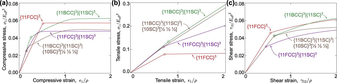
The stress–strain responses of the four trusses of interest in compression are shown in Fig. 6(a), all for truss size n = 11. Videos showing truss deformation are provided in the Supplementary Material. Stress is normalized by E oρ2 and strain is normalized by ρ. These normalizations yield the expected scalings in properties, notably stiffness proportional to E oρ and buckling strength proportional to E oρ2. Provided ρ is sufficiently small and failure is buckling-dominated (i.e., neither yielding nor fracture intervene), the results in this form are, to a very good approximation, independent of ρ and E o. This feature is illustrated in Fig. S2 in the Supplementary Material.
Stress–strain responses of trusses subjected to (a) uniaxial compression, (b) uniaxial tension, and (c) pure shear. (See also Videos VIDS. S3–S6 in the Supplementary Material.)
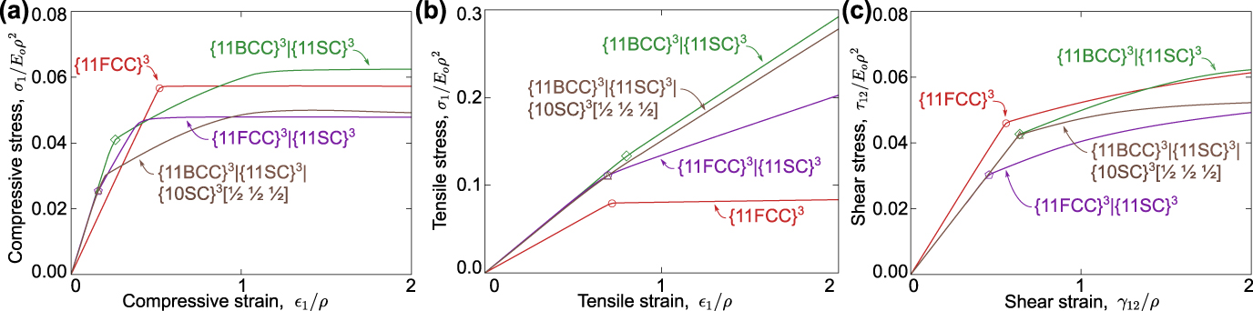
The {FCC} truss exhibits the lowest modulus but highest initial buckling stress [Fig. 6(a)]. Buckling occurs within 2/3 of the struts (types I and II); the remainder (type III) experiences tension. Buckling initiates and proceeds at a stress σ1/E oρ2 ≈ 0.057. This yields an essentially elastic, perfectly plastic behavior.
Although the addition of the {SC} truss to the {FCC} truss is required to produce an elastically isotropic (binary) truss, the addition has a detrimental effect on strength. In the {FCC}|{SC} truss, type IV struts within the {SC} sub-truss buckle first, at a stress σ1/E oρ2 ≈ 0.03. As buckling of these struts proceeds, the tangent modulus decreases only slightly because the {FCC} struts remain unbuckled. The latter struts subsequently buckle, at stress σ1/E oρ2 ≈ 0.048: about 20% lower than that of the elementary {FCC} truss. At this point, essentially all of the load is borne by the {FCC} struts.
The binary {BCC}|{SC} exhibits a similar sequence of buckling events, albeit at higher stresses; the {SC} and {BCC} struts buckle at stresses σ1/E
oρ2 ≈ 0.041 and 0.062, respectively. The latter exceeds the strength of the elementary {FCC} truss by about 10%. This effect could be exploited in practice only if the strut material were to have sufficiently high yield and fracture strains, thereby allowing the struts to remain elastic up to the second buckling event. The ternary
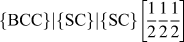 $\left\{ {{\rm{BCC}}} \right\}|\left\{ {{\rm{SC}}} \right\}|\left\{ {{\rm{SC}}} \right\}\left[ {{1 \over 2}{1 \over 2}{1 \over 2}} \right]$
truss exhibits the lowest buckle-initiation stress.
B. Tension (n = 11)
All trusses undergo compressive strut buckling when the applied load is tensile [Fig. 6(b)]. The {FCC} truss exhibits the lowest modulus and the lowest buckling stress. Buckling initiates and proceeds at σ1/E oρ2 ≈ 0.079: 40% greater in magnitude than the corresponding compressive strength. The strength differential is attributable to the fraction of buckling struts: 1/3 in tension (type III) and 2/3 in compression (strut types I and II). The balance of struts—2/3 in tension and 1/3 in compression—provides stabilization against buckling.
Strut buckling in the compound trusses leads to only a modest reduction in tangent modulus and a bilinear stress–strain response. The secondary tangent modulus is governed by the struts that are aligned with the loading direction and that bear most of the load. Buckling begins in the {FCC}|{SC} truss at essentially the same strain as that of the elementary {FCC}. But, because the stiffness of the compound truss is higher (by about 15%), the buckling stress is higher by a proportionate amount (also 15%).
The {BCC}|{SC} truss exhibits the highest strength, governed by buckling of type V {SC} struts. In comparison to the {SC} struts in the {FCC}|{SC} and the
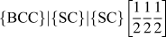 $\left\{ {{\rm{BCC}}} \right\}|\left\{ {{\rm{SC}}} \right\}|\left\{ {{\rm{SC}}} \right\}\left[ {{1 \over 2}{1 \over 2}{1 \over 2}} \right]$
trusses, type V {SC} struts have the lowest slenderness ratio.
C. Shear (n = 11)
The responses in shear are plotted in Fig. 6(c). Here, the same normalizations are used for stress and strain: E oρ2 and ρ, respectively. (Note that when stretch-dominated trusses are loaded in shear, the struts experience only axial loads, and hence their stresses are dictated by E o, not G o.)
The {FCC} truss exhibits the highest initial stiffness and the highest buckling stress [Fig. 6(c)]. Buckling initiates in type III struts at τ12/E oρ2 ≈ 0.046. Thereafter, the tangent modulus decreases by about 80% and the stress continues to increase as the type I struts are stretched further. In the {FCC}|{SC} truss, the modulus and the buckling strain are each reduced by 20% relative to those of the elementary {FCC} truss. As a result, the {FCC} struts in the compound truss buckle at an applied stress that is about 64% that of the {FCC} truss. Here, again the addition of {SC} to {FCC} to produce an isotropic binary truss comes at the expense of a significantly reduced strength.
The {BCC}|{SC} and the
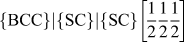 $\left\{ {{\rm{BCC}}} \right\}|\left\{ {{\rm{SC}}} \right\}|\left\{ {{\rm{SC}}} \right\}\left[ {{1 \over 2}{1 \over 2}{1 \over 2}} \right]$
trusses buckle at the same stress: τ12/E
oρ2 ≈ 0.043. This is because the {BCC} sub-trusses in the two compound trusses are equivalent. Here, the {SC} struts make no significant contribution to the response prior to buckling. Only after the {BCC} struts buckle do the {SC} struts engage and the curves for the two trusses begin to diverge.
D. Effects of truss size on strength
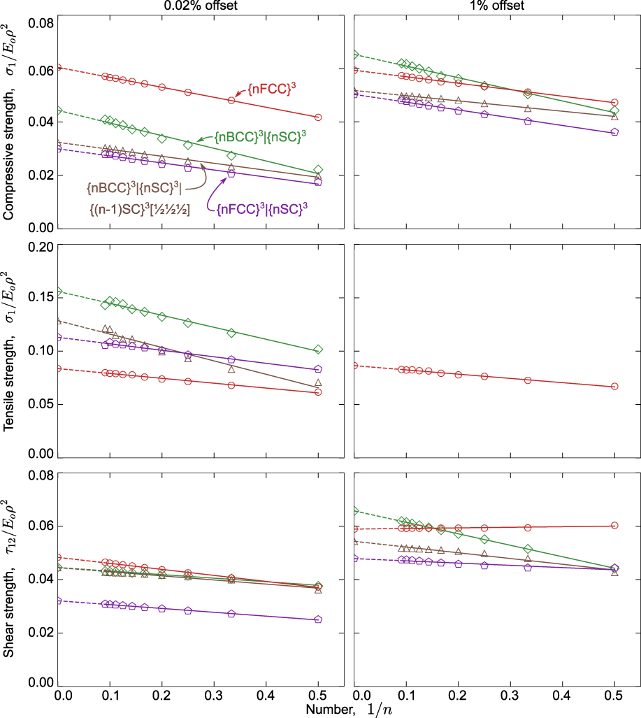
In light of the nonlinear behavior obtained in the post-buckling domain, truss strengths are characterized using offset stresses at two strains: 0.02 and 1%. Effects of truss size are shown in Fig. 7. Here, the strengths are plotted against 1/n. (Although this selection was based in part on the observation that the fraction of struts at the free boundaries is proportional to 1/n, the effects of n on strength are not due entirely to boundary effects as discussed below.) In this form, the strengths vary essentially linearly with 1/n. Linear extrapolation to 1/n = 0 yields the expected strengths of infinitely large trusses.
Strengths of trusses, defined at 0.02 and 1% offset strains.
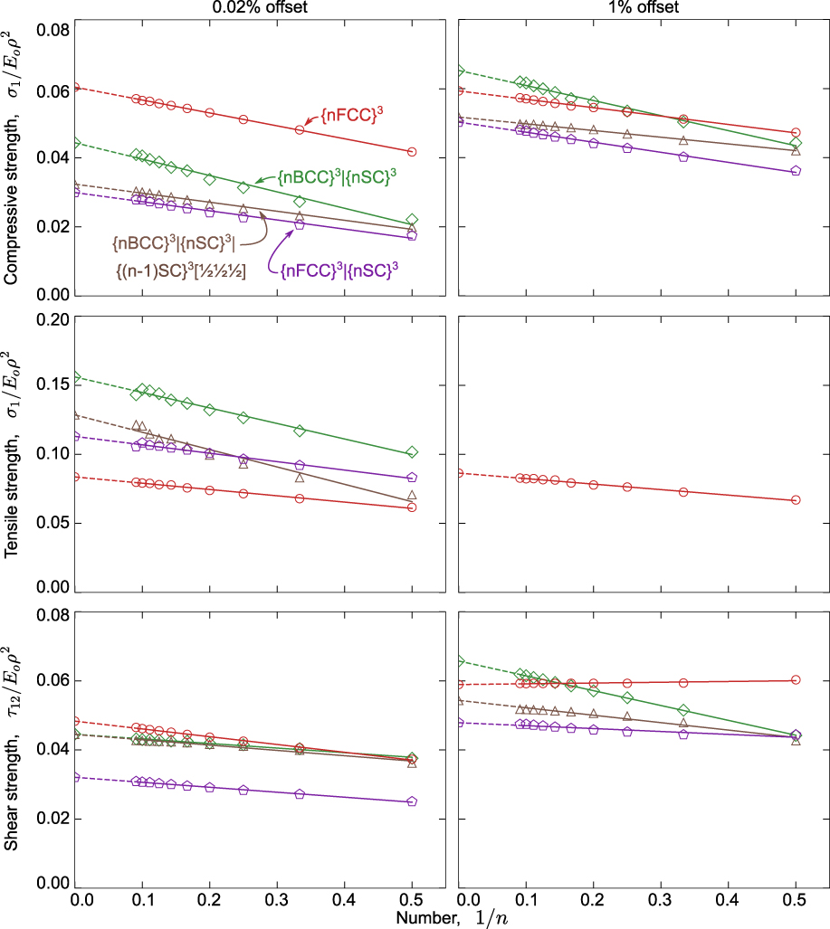
The offset stresses for the {FCC} truss in tension and compression are the same at both the 0.02 and 1% levels, a result of the elastic, perfectly plastic behavior in these two loadings. In shear, the two differ slightly because of the hardening caused by stretching of type I struts after type II struts have buckled.
The behaviors of the compound trusses in compression are more nuanced. Here, there are two distinct buckling events in the constituent sub-trusses; the 0.02% offset captures the first, whereas the 1% offset captures the second. With the hardening that occurs between the two buckling events, the 1% offset strengths for the compound trusses become comparable to those for the {FCC} truss. Indeed, for large trusses, the {BCC}|{SC} is slightly stronger than the {FCC} (by about 10%).
Although the linear dependence of strength on 1/n appears to coincide with the scaling of the fraction of struts that are affected by boundaries, the size dependence is due at least in part (perhaps largely) to the variations in strut slenderness ratio with n. That is, to have circular struts along the truss faces and edges while maintaining a constant relative density, the strut slenderness must be adjusted to reflect changes in n. For example, l/r in the {FCC} truss goes from about 63 to 52 as n goes from 1 to infinity. Analogous adjustments must be made to maintain the same volume fractions in the compound trusses. For example, the slenderness ratio of the {SC} struts in the {BCC}|{SC} truss goes from 97 to 49 as n goes from 1 to infinity. The slenderness ratio of the {BCC} struts in this truss remains constant throughout since these struts are contained entirely within the truss interior. The increase in slenderness ratio with decreasing n must play a central role in the reported dependence of strength on truss size.
E. Effective-length factors and buckling metrics
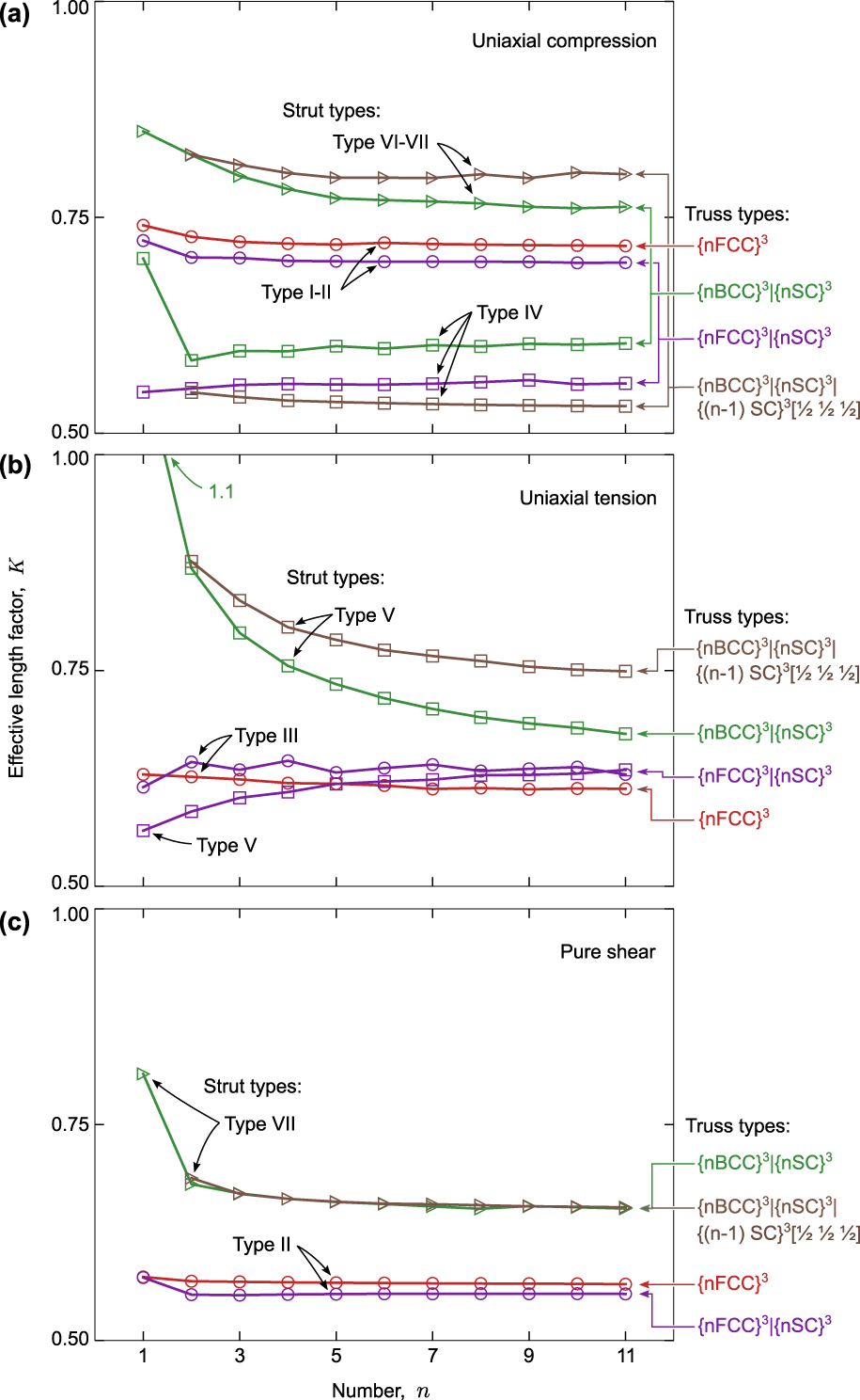
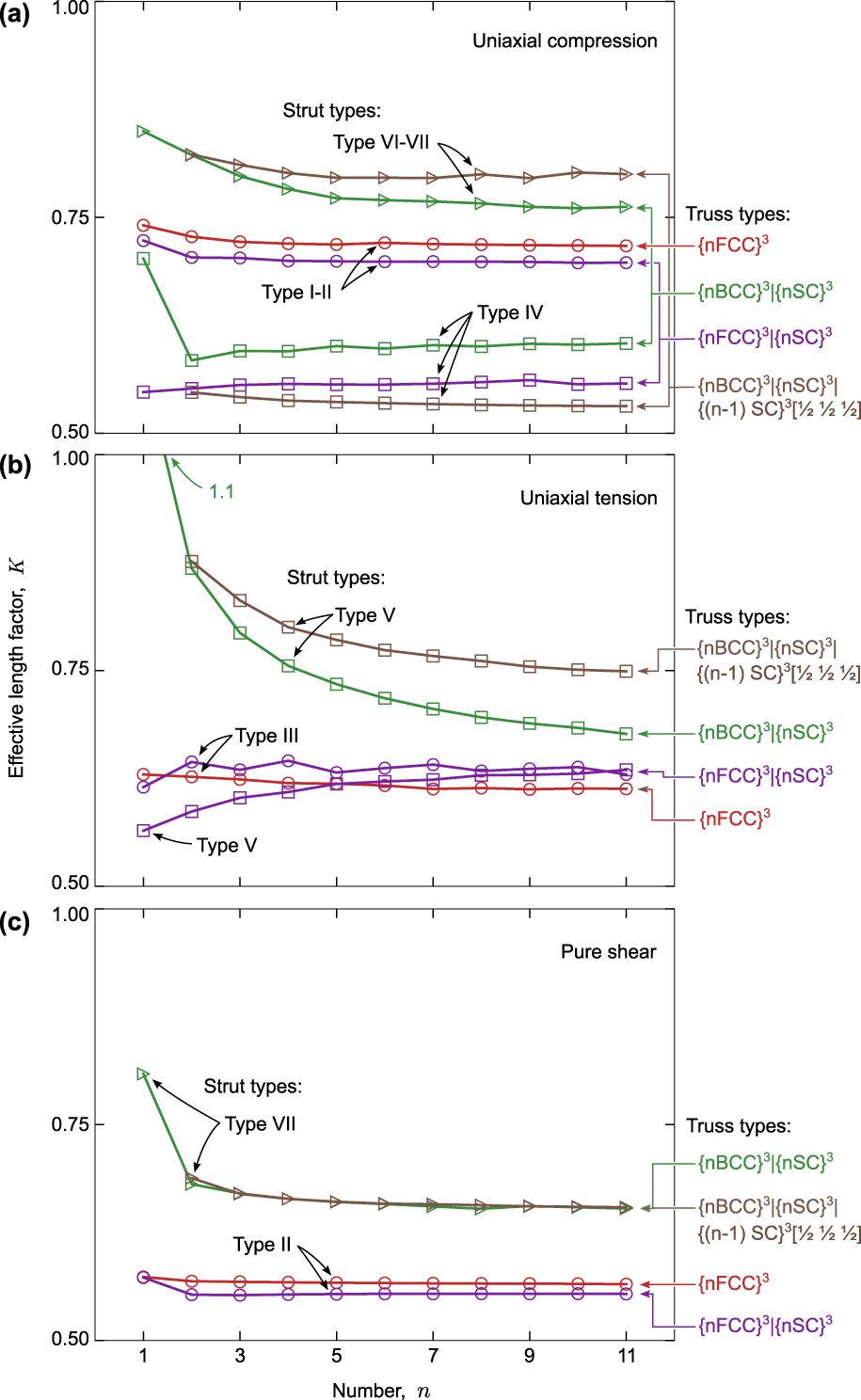
Effective-length factors K (inferred from truss strength, strut strain, and strut slenderness ratio) are, to a very good approximation, independent of n when n > 5 (Fig. 8). Values of K in this domain for each strut population are summarized in Tables I–III.
Effective length factors of various strut populations when trusses are loaded in (a) uniaxial compression, (b) uniaxial tension, and (c) pure shear.
Strut strains, buckling metrics, and truss strengths for shear loading.
In uniaxial compression, K is lowest for type IV {SC} struts within the compound trusses and falls in the narrow range of 0.53–0.60. Being close to 1/2, these values indicate that the end conditions on the struts resemble those of a strut that is fully constrained at both ends. Values of K for other struts are somewhat higher, falling in the range 0.7–0.8. Specific values depend on the fraction of struts that are undergoing buckling and the fraction of struts that experience tension.
In the elementary {FCC} truss, K = 0.72, 0.61, and 0.58 in compression, tension, and shear, respectively. The differences are attributable to the lower fraction of struts that buckle in shear and tension relative to that in compression: only 1/3 in shear (strut type I) and tension (type III), and 2/3 in compression (strut types I and II). The balance of struts—2/3 in shear and tension and 1/3 in compression—provides stabilization against buckling. Comparable differences are obtained in the {FCC} sub-truss within the compound trusses. Here, again the differences are attributable to the fractions of buckling struts.
Similar trends are obtained in the {BCC} sub-truss within the two compound trusses. For example, in the {BCC}|{SC} binary, K is higher in compression (0.76) than in shear (0.65), again reflecting the fraction of buckling struts: 100% in compression and 50% in shear.
Finally, examination of the buckling metrics (Tables I–III) provides additional insights into the sequence of buckling events and their manifestations in the stress–strain responses. In compression, for example, the ranking of stresses and strains at the 0.02% offset follows in accordance with the buckling metric βc: the lowest values associated with buckling of the {SC} struts in the {FCC}|{SC},
 $\left\{ {{\rm{BCC}}} \right\}|\left\{ {{\rm{SC}}} \right\}|\left\{ {{\rm{SC}}} \right\}\left[ {{1 \over 2}{1 \over 2}{1 \over 2}} \right]$
, and {BCC}|{SC} trusses (βc = 0.07ρ, 0.08ρ, and 0.12ρ, respectively), followed by buckling in the elementary {FCC} truss βc = 0.22ρ). Whereas all struts in the {FCC} buckle simultaneously and hence lead to a constant buckling stress, the compound trusses continue to “harden”, until the second population of compressed struts buckles (βc = 0.38ρ and 0.35ρ in {BCC}|{SC} and
 $\left\{ {{\rm{BCC}}} \right\}|\left\{ {{\rm{SC}}} \right\}|\left\{ {{\rm{SC}}} \right\}\left[ {{1 \over 2}{1 \over 2}{1 \over 2}} \right]$
, respectively). Similar correlations are evident upon examination of the buckling sequences under tensile and shear loading [Figs. 6(b) and 6(c)] along with the metrics βt and βs (Tables II and III).
VI. SUMMARY AND CONCLUSIONS
Families of stiff isotropic compound trusses based on binary and ternary combinations of elementary cubic trusses have been identified. Each exhibits the maximal axial stiffness for isotropic trusses. Reference Gurtner and Durand25 The stiffnesses of some of these trusses are not simply the additive sums of the contributions from the constituent sub-trusses. Instead, mechanical coupling between the constituent elementary trusses enables more efficient strut loading and leads to increased stiffness. This behavior is best exemplified by the 60% {BCC}|40% {SC} truss, wherein the Young’s modulus is over 20% greater than the rule-of-mixtures prediction.
The effects of truss topology and geometry on buckling strength can lead to three distinct effects: (i) the axial strains within buckling struts, (ii) the slenderness ratio of buckling struts, and (iii) the buckling constraints at the strut ends, manifested in the effective length factors. The three factors are combined into buckling metrics for the three loading scenarios. This partitioning of effects yields new insights into the connections between truss topology and truss strength. Based solely on geometric complexity, binary compound trusses are preferable over ternaries. Binary trusses are also superior to ternaries in terms of their inelastic response. The latter differences stem from the fact that, to maintain a fixed relative density, the slenderness ratio of some of the struts must be increased when expanding the design from binary to ternary trusses. The increase in nodal connectivity associated with the third truss does not provide sufficient benefit to offset the detrimental effects of higher strut slenderness ratios.
Boundary effects persist roughly two unit cell lengths into the truss from the surface. There, reduced nodal constraint leads to a dispersion in strut strains. It is in these regions that strut buckling initiates. Although boundary effects do not play a dominant role in the buckling strengths of the present trusses, they would naturally affect other failure modes. That is, if failure were to occur by strut yielding or fracture, strain amplifications in the near-boundary regions could reduce truss strengths substantially relative to those expected on the basis of average strut strains in the bulk of the truss.
The {BCC}|{SC} truss is competitive with the {FCC} truss in several respects. In addition to being isotropic with maximal stiffness, it exhibits compressive and shear strengths that are comparable to those of the {FCC} for large offset strains as well as higher strength in tension. Achieving the higher strengths is predicated, however, on the material having sufficiently high yield and tensile fracture strain; otherwise, strut yield or fracture would govern strength.
Supplementary Material
To view supplementary material for this article, please visit https://doi.org/10.1557/jmr.2018.2.
ACKNOWLEDGMENTS
This work was supported by the Institute for Collaborative Biotechnologies through grant W911NF-09-0001 from the U.S. Army Research Office. The content of the information does not necessarily reflect the position or the policy of the Government, and no official endorsement should be inferred.