3.1. Typical flow structure

We first examine the characteristic flow structure in a cell with aspect ratio $\varGamma = 10$ . The flow typically organises into multiple convection rolls aligned in the horizontal direction. Among these configurations, a six roll structure is the most frequently observed one and emerges spontaneously within the present parameter space. A representative long time averaged velocity field, obtained by averaging over three hours at $Ra = 3.5 \times 10^8$ and $\textit{Pr} = 9.9$ , is shown in figure 2(a). It is evident that the mean flow comprises six horizontally aligned convection rolls. These rolls differ slightly in size as revealed by their horizontal extents and velocity distributions. Small corner rolls appear near the upper left and upper right regions of the domain. Such secondary corner rolls have also been reported in smaller aspect-ratio systems (Xia, Sun & Zhou Reference Xia, Sun and Zhou2003; Sugiyama et al. Reference Sugiyama, Ni, Stevens, Chan, Zhou, Xi, Sun, Grossmann, Xia and Lohse2010; Huang & Xia Reference Huang and Xia2016; Chen et al. Reference Chen, Huang, Xia and Xi2019; Zhao et al. Reference Zhao, Wang, Wu, Chong and Zhou2022; Li, Chen & Xi Reference Li, Chen and Xi2024a ). A closer examination of the leftmost roll in figure 2(a) shows the presence of internal substructures. These features resemble the abnormal single roll state documented by Chen et al. (Reference Chen, Huang, Xia and Xi2019, Reference Chen, Wang and Xi2020) and Kar et al. (Reference Kar, Kumar, Das and Lakkaraju2020). The maximum flow speed occurs near the top and bottom conducting plates. This spatial velocity distribution is consistent with observations from flattened convection cells (Qiu & Tong Reference Qiu and Tong2001; Xia et al. Reference Xia, Sun and Cheung2008; Li et al. Reference Li, Chen, Xu and Xi2022, Reference Li, Chen and Xi2024b ). Because the horizontal flow near the plates is confined to a narrower vertical section compared with the vertical flow near the sidewalls, conservation of mass requires both direction to transport equal volume flux. As a result, the horizontal velocity near the conducting plates must be greater than the vertical velocity adjacent to the sidewalls. The relation between roll size and characteristic velocity is examined in detail in § 3.2. Another important feature is that adjacent rolls display horizontal velocities of opposite sign at the same vertical position. This alternating pattern provides a convenient way to identify neighbouring rolls. To quantify this spatial variation, we extract the horizontal velocity along a line located $1\ \text{cm}$ above the bottom plate, i.e. at $z = 1\ \text{cm}$ . This height is chosen because the horizontal velocity is nearly maximal at this location. The resulting profile is shown in figure 2(b), where both the horizontal velocity $u$ and its absolute value $\left \lvert u \right \rvert$ are plotted as functions of $x$ . Local minima in $\left \lvert u \right \rvert$ correspond to roll boundaries and are marked by green dots, which provide a direct measure of the roll width. The temporal evolution of the number, size and position of the rolls is illustrated by the horizontal velocity map in figure 2(c), where alternating colour bands delineate the roll structures over time.

In our experiments, the six-roll structure aligned horizontally is the most commonly observed and representative flow state in the $\varGamma = 10$ cell. However, this configuration is not unique. We find that for identical $(Ra, \textit{Pr})$ combinations, the flow can spontaneously evolve into different states with varying numbers of horizontally aligned rolls. In figure 3, we present flow states that differ from those shown in figure 2 at idential control parameters, $Ra = 3.5 \times 10^8, \textit{Pr} = 9.9$ . It should be emphasised that figures 2 and 3 represent two completely independent experiments conducted under identical initial conditions. Both experiments began from a static state that the working fluid was first kept in a quiescent state for at least six hours before initiating the experiment. This procedure ensured that the system was free of residual motion and that the observed flow structures are not influenced by the flow history. In figure 3(a), we show the time series of horizontal velocity and one can see that the flow spontaneously evolves from four-roll state to five-roll state around $t= 9300\ \text{s}$ . Two representative snapshots of short time averaged velocity fields are displayed in figures 3(b) and 3(c), corresponding to four-roll and five-roll states, respectively. The short time averaged velocity fields are obtained by averaging over one turnover time $t_E$ . The turnover time $t_E$ is estimated from the maximum instantaneous velocity and the average perimeter of an individual convection roll. For an instantaneous flow field having a maximum horizontal velocity $u_0$ , we define the average perimeter of a single roll as $C = ((n + 1) \times H + 2L) / n$ , where $n$ is the number of convection rolls. This yields an estimate $t_E = C / u_0$ . These stable configurations, namely the six rolls state shown in figure 2(a), the four rolls state shown in figure 3(b) and the five rolls state shown in figure 3(c) clearly demonstrate the coexistence of multiple flow states under identical control parameters.

Figure 3.

(a) Space–time plot of horizontal velocity $u$ along $z = 1\,\text{cm}$ for $Ra = 3.5 \times 10^8, \textit{Pr} = 9.9$ . The free fall time is approximately $t_f \approx 1.25$ s and the total duration shown corresponds to more than $10^4$ free fall times. Vertical dashed lines indicate the times at which short-time-averaged velocity fields are extracted. (b,c) Velocity fields averaged over one turnover time $t_E$ , showing (b) a four-roll state and (c) a five-roll state. Colour represents the in-plane velocity magnitude $(u^2 + w^2)^{1/2}$ .

One may ask how the transition occurs in figure 3. From figure 3(a), it can be seen that a new roll emerges from the right side, where a large roll previously occupied approximately $40\,\%$ of the cell length. Previous studies (Wang et al. Reference Wang, Verzicco, Lohse and Shishkina2020b ; Zwirner et al. Reference Zwirner, Tilgner and Shishkina2020) have shown that rolls with large aspect ratio are likely to break up due to elliptic instability. This suggests that the transition observed here may be related to such instabilities. The relevant question is whether the flow would transition to other states if the experiment shown in figure 3 were conducted for a longer duration. Theoretically, it is possible that, sooner or later, there will be a transition. While it should be emphasised that in our experiments, once a flow state is established, spontaneous transition from one state to another state is very rare. Another interesting observation is that, in each of the observed cases, the rolls are not in equal size, and the largest roll grows noticeably in size as the total number of rolls decreases. The variable sizes of rolls are reproducible, although the largest or smallest rolls are not at the same position for each experiment. In our experiments, the flow field that consists of uniformly sized rolls has never been observed.

To further examine whether the occurrence of multiple flow states is related to the insufficient turbulence intensity, we increase the $Ra$ by more than one order of magnitude. This is achieved by using 0.65 cSt silicone oil as the working fluid. Figure 4 shows representative short time averaged flow fields at $Ra = 7.2 \times 10^9$ and $\textit{Pr} = 9.9$ . Even with a Rayleigh number $Ra$ that is approximately twenty times larger, the system still exhibits multiple stable flow states. Specifically, a five-roll configuration is shown in figure 4(a) and a triple-roll configuration is shown in figure 4(b). These observations confirm that multiple flow states persist even when the turbulence intensity is significantly increased. The flow structures at this higher $Ra$ remain dominated by flattened vortices with different horizontal extent. It should be noted that although $Ra$ is relatively higher for the flow states shown in figure 4, the flow fields appear more stable compared with the flow states shown in figure 3. This is due to that when $Ra$ is relatively low, the inner core of the convection rolls can undergo breakup, resulting in the emergence of substructures within a single roll, as shown in figure 3(b,c). These internal substructures make the flow field at lower $Ra$ appear more disturbed even after time averaging. Such substructures are characteristic features in confined geometries at intermediate $Ra$ (Chen et al. Reference Chen, Huang, Xia and Xi2019). When comparing figures 2, 3 and 4, a clear trend emerges. The number of rolls that can stably exist decreases as $Ra$ increases. In other words, the characteristic length scale of the flow structures increases with $Ra$ . This trend is consistent with previous studies (Hartlep, Tilgner & Busse Reference Hartlep, Tilgner and Busse2003; Akashi et al. Reference Akashi, Yanagisawa, Tasaka, Vogt, Murai and Eckert2019).

Figure 4.

Velocity fields averaged over one turnover time $t_E$ , showing (a) a five-roll state and (b) a triple-roll state at $Ra = 7.2 \times 10^9, \textit{Pr} = 9.9$ . Colour represents the in-plane velocity magnitude $(u^2 + w^2)^{1/2}$ .

To assess the generality of the multiple flow states, we also examine the flow field for different $\textit{Pr}$ . Aqueous glycerol solutions of different concentrations are used to systematically adjust $\textit{Pr}$ . We observe that multiple flow states occur over a wide range of $\textit{Pr}$ from 4.3 to 67.3, which indicates that their coexistence is not confined to a specific value of $\textit{Pr}$ . In figure 5, we present typical flow fields for $\textit{Pr} = 18.3$ and $\textit{Pr} = 67.3$ at similar $Ra$ . For $\textit{Pr} = 18.3$ , the flow field exhibits a structure similar to that of the $\textit{Pr} = 9.9$ cases discussed previously. When $\textit{Pr}$ is further increased to 67.3, a clear difference is that the number of roll-like structures present in the flow field appears much larger than in the lower $\textit{Pr}$ cases. It should be noted that we use the term roll-like structure for the $\textit{Pr} = 67.3$ case, since even with the aid of streamlines, the flow structures are not as well defined as the rolls in the lower $\textit{Pr}$ cases. However, we would still count these roll-like structures as rolls when we analyse how the number of rolls changes with $\textit{Pr}$ .

Now, we can map out the flow state diagram for flow states that evolve spontaneously (without controlled perturbations) in the parameter space of $Ra$ and $\textit{Pr}$ , as shown in figure 6. The procedure used to explore multiple states in figure 6 is the same for all parameters. Each experiment began from a static state in which the working fluid was kept quiescent for at least six hours before the experiment. For each ( $Ra$ , $\textit{Pr}$ ) combination shown in figure 6, we performed approximately ten independent experimental realisations. In each realisation, a short-duration (typically approximately 10 minutes) PIV measurement was first conducted after the temperatures of the top and bottom plates had stabilised to identify the current flow state. Extended PIV measurements, with a duration of at least two hours, were carried out only for those realisations that exhibited flow states different from previously measured cases. Since parameter scanning is very time consuming, the data shown in figure 6 represent what we have been able to accomplish thus far. The phase diagrams in figure 6(a–e) for different $\textit{Pr}$ collect the number of rolls of the experimentally observed stable configurations and demonstrate the robust existence of multiple flow states in the $\varGamma = 10$ cell. In figure 6(f), we plot the arithmetic mean of the data points shown in the phase diagrams as a function of $\textit{Pr}$ . The average number of rolls remains nearly unchanged for $4.3 \leqslant \textit{Pr} \leqslant 18.3$ and increases significantly when $\textit{Pr}$ reaches 67.3. These results suggest a transition in the flow organisation at large $\textit{Pr}$ . There is a clear discrepancy between the lower $\textit{Pr}$ cases and the case with $\textit{Pr} = 67.3$ with respect to the flow field. As stated in the previous paragraph, the largest velocity occurs near the horizontal plates and is primarily in the horizontal direction for the lower $\textit{Pr}$ cases, whereas in figure 5(b) for $\textit{Pr} = 67.3$ , the largest velocity is in the vertical direction between roll like flow structures. This discrepancy implies that the flow may enter a new regime in which vertical motion dominates the flow field. This behaviour is consistent with the flow field reported by Wang et al. (Reference Wang, Chen, Xu and Xi2024) at high $\textit{Pr}$ , where the flow is dominated by thermal plumes rather than by the large-scale circulations. We must emphasise that the phase diagram in figure 6 does not represent an exhaustive enumeration of all possible flow states. A comprehensive understanding of the full range of possible roll states will require further systematic investigation. Such an investigation may be carried out most effectively with the aid of experimental experience in other systems, for example, Huisman et al. (Reference Huisman, van der Veen, Sun and Lohse2014) conducted in the Taylor–Couette system, or through numerical simulations.

Figure 5.

Multiple flow states at different $\textit{Pr}$ numbers. (a) Seven-roll state and six-roll state at $Ra = 2.05 \times 10^8$ , $\textit{Pr}=18.3$ , respectively. (b) Roll-like flow structures at $Ra = 1.63 \times 10^8$ , $\textit{Pr}=67.3$ . By naked eyes, the number of roll-like structures are 18 and 21 respectively in the upper and lower panels.

Regarding the spontaneously occurring multiple states, our experiments reveal two scenarios. One scenario is that the flow selects one flow state when it is initiated from a quiescent state. The other scenario is that the flow spontaneously transitions from one well-formed state, which remains stable for a long time, to another distinct state, as shown in figure 3. In our experiments, such spontaneous transitions from one state to another are rare, but they can still be observed occasionally. Regarding this phenomenon, a comparison between low- $\textit{Pr}$ and moderate- to high- $\textit{Pr}$ regimes could be interesting. Flow measurements in a rectangular cell with an aspect ratio of 5 show that parallel convection rolls form the basic flow pattern when $\textit{Pr} \lt 1$ (Yanagisawa et al. Reference Yanagisawa, Yamagishi, Hamano, Tasaka, Yoshida, Yano and Takeda2010). In that configuration, spontaneous flow reversals and transitions between different roll regimes occur more frequently (Yanagisawa et al. Reference Yanagisawa, Yamagishi, Hamano, Tasaka and Takeda2011; Akashi et al. Reference Akashi, Yanagisawa, Tasaka, Vogt, Murai and Eckert2019) than in the present experiments. This difference can be attributed to the combined effects of low viscosity, high thermal diffusivity and strong inertial forces in liquid metals, which promote intense turbulent fluctuations and facilitate transitions between different roll states. In contrast, moderate- to high- $\textit{Pr}$ fluids have higher viscosity and lower thermal diffusivity, which may suppress fluctuations and stabilise the flow structures. This difference in flow physics explains why spontaneous transitions are rare in our experiments despite the much higher  $Ra$ .

Figure 6.

(a–e) Phase diagram showing the number of horizontally aligned rolls $n$ as a function of Rayleigh number $Ra$ for different Prandtl number $\textit{Pr}$ . Each data point corresponds to an experimentally observed stable roll configuration. (f) Arithmetic mean of the number of horizontally aligned rolls $n$ obtained from panels (a–e) as a function of the Prandtl number $\textit{Pr}$ . The dashed line represents $n = 6$ .

Although the presence of multiple flow states is consistent with findings from two-dimensional numerical simulations (Wang et al. Reference Wang, Verzicco, Lohse and Shishkina2020b , Reference Wang, Wan and Sun2018, Reference Wang, Chong, Stevens, Verzicco and Lohse2020a ), the number of rolls that stably exist in experiments is significantly lower than that predicted in simulations. Wang et al. (Reference Wang, Verzicco, Lohse and Shishkina2020b ) showed that imposing different initial conditions leads to different stable flow states in two-dimensional simulations and the mean aspect ratio of individual rolls, $\varGamma _r = \varGamma / n$ , lies within $2/3 \leqslant \varGamma _r \leqslant 4/3$ , where $n$ denotes the number of rolls. According to this relation, a system with $\varGamma = 10$ should permit at least eight rolls, which exceeds the number observed in our experiments. They also found that $\varGamma _r$ decreases as $Ra$ increases, implying that the number of rolls should grow with $Ra$ . In contrast, our experiments show that the number of rolls tends to decrease with $Ra$ . For example, for $\textit{Pr} = 9.9$ , one can see that with increasing $Ra$ , the number of rolls can decrease to three. This implies that the discrepancy between the numerical results and the experimental observations is expected to become more pronounced at higher $Ra$ . The simulations employed horizontal periodic boundary conditions, which imply infinite length in the horizontal direction, while our experiments have rigid walls. It is therefore reasonable to conjecture that the difference in the number of rolls may arise from the different boundary conditions and the sidewall boundary condition appears to play an essential role in determining the number of stable rolls. This interpretation is supported by Wang et al. (Reference Wang, Wan and Sun2018), who found that the number of stable rolls decreases when the periodic boundary condition is replaced by solid sidewalls. Specifically, for $Ra = 10^7$ and $\textit{Pr} = 0.71$ , they reported 5–8 rolls for $\varGamma = 8$ and 7–12 rolls for $\varGamma = 12$ . Even for the same boundary conditions, the number of stable rolls in simulations remains higher than in experiments. A more plausible explanation lies in the difference in dimensionality between simulations and experiments. Experimental systems are inherently three-dimensional and the lateral extent of the cell, denoted by $\varGamma _{\textit{lateral}} = W / H$ , introduces additional disturbance that are absent in 2-D simulations. For comparable Rayleigh numbers ( $Ra \sim 10^8$ ), the influence of $\varGamma _{\textit{lateral}}$ can be assessed from previous studies. In the current experiments with $\varGamma _{\textit{lateral}} = 0.3$ , the number of spontaneously generated rolls were predominantly in the range of 4–7, corresponding to the $\varGamma _r$ in a range of $10/7 \leqslant \varGamma _r \leqslant 5/2$ . Xia et al. (Reference Xia, Sun and Cheung2008) reported that in a rectangular cell with $\varGamma = 9.9$ and $\varGamma _{\textit{lateral}} = 2.5$ , the turbulent structure consisted of three horizontally aligned rolls, with the average size of the roll having $\varGamma _r \approx 3.3$ . In systems with even larger $\varGamma _{\textit{lateral}}$ , often referred to as mesoscale convection, the flow develops into turbulent superstructures with substantially larger roll sizes, typically $\varGamma _r \geqslant 6$ (Pandey, Scheel & Schumacher Reference Pandey, Scheel and Schumacher2018; Stevens et al. Reference Stevens, Blass, Zhu, Verzicco and Lohse2018; Green et al. Reference Green, Vlaykov, Mellado and Wilczek2020; Krug, Lohse & Stevens Reference Krug, Lohse and Stevens2020; Pandey et al. Reference Pandey, Krasnov, Sreenivasan and Schumacher2022; Moller et al. Reference Moller, Käufer, Pandey, Schumacher and Cierpka2022). These observations consistently indicate that roll size increases with the expansion of the third dimension. This provides a straightforward explanation for the observed discrepancy between experiments and two-dimensional simulations regarding both the number and the size of roll structures. However, it should be noticed that our cell with $\varGamma _{\textit{lateral}} = 0.3$ is a confined geometry where flow organisation can differ substantially from that in cells with larger $\varGamma _{\textit{lateral}}$ . The narrow lateral extent acts as a stabilising constraint that enhances the coherence of the large-scale circulation and suppresses certain three-dimensional instabilities (Huang et al. Reference Huang, Kaczorowski and Xia2013; Huang & Xia Reference Huang and Xia2016; Chong et al. Reference Chong, Yang, Huang, Zhong, Stevens, Verzicco, Lohse and Xia2017). This confinement likely contributes to the stability and persistence of the roll states we observe. Meanwhile, in our narrow geometry, the no-slip lateral sidewalls generate a secondary flow perpendicular to the roll axis that is absent in both 2-D simulations and wider cells. As demonstrated by Vogt et al. (Reference Vogt, Ishimi, Yanagisawa, Tasaka, Sakuraba and Eckert2018), Yang, Vogt & Eckert (Reference Yang, Vogt and Eckert2021), this secondary circulation can significantly influence roll stability and the development of instabilities.

3.2. Reynolds number

An interesting question concerning the multiple-roll configuration in a $\varGamma = 10$ cell is whether a systematic relationship exists between $\textit{Re}$ and the size of the rolls. To investigate this relationship, we first extract the individual rolls using the method illustrated in figure 2(b). The size of each roll is then determined and all velocity data enclosed within its boundaries are extracted. Once the roll sizes are obtained, the aspect ratio of each roll is defined as $\varGamma _{\textit{roll}} = W_{\textit{roll}}/H$ , where $W_{\textit{roll}}$ denotes the roll width and $H$ is the cell height. All rolls in our experiments share the same height $H$ . Only cases in which the rolls remain stable for at least one hour during data acquisition are included in the analysis. The stability of the rolls is assessed from the space–time plot of the horizontal velocity $u$ along $z = 1\ \text{cm}$ , for example, figure 2(c), which shows no significant variation for at least one hour.

Figure 7.

$\textit{Re}$ as function of $\varGamma _{\textit{roll}}$ at different $Ra$ and $\textit{Pr}$ . (a) $\textit{Re}_{u,\textit{roll}} = \sqrt {\langle u^2 \rangle _{\textit{roll}}} H / \nu$ based on horizontal velocity. (b) $\textit{Re}_{w,\textit{roll}} = \sqrt {\langle w^2 \rangle _{\textit{roll}}} H / \nu$ based on vertical velocity. (c) $\textit{Re}_{w,\textit{roll}} / \textit{Re}_{u,\textit{roll}}$ (component ratio). (d) $\textit{Re}_{\textit{roll}} = \sqrt {\langle u^2 + w^2 \rangle _{\textit{roll}}} H / \nu$ based on total velocity. All data are normalised by their corresponding values at $\varGamma _{\textit{roll}} = 1.5$ .

Figure 7 presents the dependence of $\textit{Re}$ on $\varGamma _{\textit{roll}}$ . Although the data are scattered across the various experimental conditions, the overall trends are consistent. The scatter likely reflects the limited number of datasets. Panels (a), (b) and (d) display the Reynolds numbers based on horizontal velocity $\textit{Re}_{u,\textit{roll}} = \sqrt {\langle u^2 \rangle _{\textit{roll}}} H / \nu$ , vertical velocity $\textit{Re}_{w,\textit{roll}} = \sqrt {\langle w^2 \rangle _{\textit{roll}}} H / \nu$ and total in-plane velocity $\textit{Re}_{\textit{roll}} = \sqrt {\langle u^2 + w^2 \rangle _{\textit{roll}}} H / \nu$ , respectively. Here, $\langle \rangle _{\textit{roll}}$ denotes the average taken within the boundary of each individual roll and over the time interval during which the roll structure remains stable. Panel (c) shows the ratio $\textit{Re}_{w,\textit{roll}} / \textit{Re}_{u,\textit{roll}}$ as a function of $\varGamma _{\textit{roll}}$ . To collapse the data obtained under different $Ra$ and $\textit{Pr}$ , all Reynolds numbers are normalised by their corresponding values at $\varGamma _{\textit{roll}} = 1.5$ . The values at $\varGamma _{\textit{roll}} = 1.5$ are not always available in the raw records. These values are therefore obtained by linear interpolation between the contiguous datasets that bracket $\varGamma _{\textit{roll}} = 1.5$ . As shown in figure 7(a), $\textit{Re}_{u,\textit{roll}}$ increases with increasing $\varGamma _{\textit{roll}}$ . In contrast, $\textit{Re}_{w,\textit{roll}}$ decreases monotonically with roll size, as shown in figure 7(b). This opposite behaviour can be understood from mass conservation. Assuming incompressibility, the horizontal and vertical volume fluxes must balance, implying $u H \sim w l$ and, hence, $w/u \sim 1/\varGamma _{\textit{roll}}$ . Accordingly, larger rolls require higher horizontal velocities and lower vertical velocities to maintain mass balance. This reciprocal relationship is captured in figure 7(c), where the ratio $\textit{Re}_{w,\textit{roll}} / \textit{Re}_{u,\textit{roll}}$ decreases systematically with increasing $\varGamma _{\textit{roll}}$ . The observed trend is consistent with two-dimensional numerical simulations of Wang et al. (Reference Wang, Verzicco, Lohse and Shishkina2020b ). A linear fit to the data in figure 7(c) yields a scaling exponent of $-0.61 \pm 0.03$ , which is very close to the exponent of $-0.68$ reported in simulations of (Wang et al. Reference Wang, Chong, Stevens, Verzicco and Lohse2020a ). The deviation of current experiments from the theoretical prediction of $w/u \sim 1/\varGamma _{\textit{roll}}$ can be attributed to the three-dimensional nature of the flow, the presence of secondary corner rolls and the mass exchange across adjacent rolls. As shown in figure 7(d), the total Reynolds number $\textit{Re}_{\textit{roll}}$ tends to increase slightly with roll size. This further indicates that the quasi-two-dimensional flow in the $\varGamma = 10$ cell is primarily driven by horizontal motion as the the total Reynolds number $\textit{Re}_{\textit{roll}}$ shares the similar trend with $\textit{Re}_{u,\textit{roll}}$ . Due to the absence of full-field temperature measurements, we are unable to determine the relationship between the $\textit{Nu}$ and roll size.

Figure 8.

(a) $Ra$ dependence of $\textit{Re}$ for different $\textit{Pr}$ . (b) Normalised $\textit{Re}$ data, scaled by the value at $Ra = 2 \times 10^8$ . (c) $\textit{Pr}$ dependence of the compensated $\textit{Re}$ .

We further investigate the dependence of global Reynolds number $\textit{Re}$ on $Ra$ across different $\textit{Pr}$ . We compute $\textit{Re}$ using the full velocity field and the complete time series for all experiments conducted under identical control parameters. The evaluation of $\textit{Re}$ is independent of the instantaneous roll number and does not distinguish between different roll states that may arise within a single run or across different realisations. The global Reynolds number is defined as $\textit{Re} = \langle \sqrt {u^2 + w^2} \rangle H / \nu$ , where $\langle \rangle$ denotes the average over the entire flow field. Figure 8 shows that $\textit{Re}$ decreases monotonically with increasing $\textit{Pr}$ and this decrease becomes particularly pronounced as $\textit{Pr}$ increases from 18.3 to 67.3. This trend coincides with a significant structural transition in the flow field. 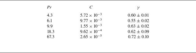At $\textit{Pr} = 67.3$ , the roll structure is no longer dominant. Instead, the flow is characterised by vertically aligned plumes. In addition to the structural transition, there is a clear change in the scaling behaviour of the Reynolds number. As indicated in table 2, the scaling exponent $\gamma$ in the relation $\textit{Re} \sim Ra^\gamma$ remains nearly constant for $4.3 \leqslant \textit{Pr} \leqslant 18.3$ , and agrees well with previous experiments and simulations conducted in quasi-2-D or 2-D systems with $\varGamma = 1$ (Sugiyama et al. Reference Sugiyama, Calzavarini., Grossmann and Lohse2009; van der Poel, Stevens & Lohse Reference van der Poel, Stevens and Lohse2013; Zhang, Zhou & Sun Reference Zhang, Zhou and Sun2017; Wang et al. Reference Wang, Verzicco, Lohse and Shishkina2020b ; Li et al. Reference Li, He, Tian, Hao and Huang2021). When $\textit{Pr}$ increases from 18.3 to 67.3, the exponent $\gamma$ increases to $0.72 \pm 0.10$ . A similar transition has been reported in both a three-dimensional (Lam et al. Reference Lam, Shang, Zhou and Xia2002; Silano, Sreenivasan & Verzicco Reference Silano, Sreenivasan and Verzicco2010) and quasi-2-D (Li et al. Reference Li, He, Tian, Hao and Huang2021) cell with $\varGamma = 1$ . In particular, the experiments of Li et al. (Reference Li, He, Tian, Hao and Huang2021) revealed that a sharp increase in the scaling exponent corresponds to the breakdown of large-scale circulation. This is consistent with the transition observed in the present study. It is worth noting that Li et al. (Reference Li, He, Tian, Hao and Huang2021) reported that the structural transition occurred at a much higher $\textit{Pr} \approx 345$ , which differs from our result. Chong & Xia (Reference Chong and Xia2016) investigated the flow field in geometrically confined domains and found that reducing the lateral aspect ratio $\varGamma _{\textit{lateral}}$ leads to distinct changes in the dominant flow regimes. As $\varGamma _{\textit{lateral}}$ decreases, the flow transitions sequentially from the classical boundary-layer-controlled regime to a plume-controlled regime and eventually to a severely confined regime. These changes are accompanied by a progressive increase in the scaling exponent of the $\textit{Re}$ . Upon entering the third regime, the large-scale circulation, which is typically formed by mushroom-like and fragmented thermal plumes, breaks down. The flow becomes dominated by long lived, vertically aligned finger like plume columns, and the scaling exponent of the $\textit{Re}$ associated with this plume-dominated state matches the value observed in the present experiment. This agreement provides further evidence that sudden changes in either the magnitude or the scaling exponent of the Reynolds number serve as reliable indicators of underlying transitions in the flow structure.

Table 2.

Fitted coefficients $C$ and scaling exponents $\gamma$ for the power-law relation $\textit{Re} = C Ra^{\gamma }$ at different $\textit{Pr}$ .

We then extract the scaling relationship of the $\textit{Re}$ with both $Ra$ and $\textit{Pr}$ by a commonly used method (Xia, Lam & Zhou Reference Xia, Lam and Zhou2002; Xie & Xia Reference Xie and Xia2017; Li et al. Reference Li, He, Tian, Hao and Huang2021). Specifically, to investigate the combined scaling $\textit{Re} \sim Ra^\gamma \textit{Pr}^\beta$ , we first normalise the $\textit{Re}$ values in each $\textit{Pr}$ group using a constant that depends on $\textit{Pr}$ . Here, the normalisation factor is taken to be the $\textit{Re}$ value at $Ra = 2 \times 10^8$ for each $\textit{Pr}$ . This procedure collapses the data across different $\textit{Pr}$ values, as shown in figure 8(b). By fitting the normalised data, we extract the scaling exponent $\gamma$ in the relation $\textit{Re} \sim Ra^\gamma$ . Next, we compensate the original $\textit{Re}$ values by dividing them by $Ra^\gamma$ and compute the average within each $\textit{Pr}$ group. This allows us to determine the scaling exponent $\beta$ in the relation $\textit{Re} \sim \textit{Pr}^\beta$ . It is important to note that data for $\textit{Pr} = 67.3$ are excluded from this analysis due to significant changes in the underlying flow structure. From the compensated data in figure 8(b), we find that $\textit{Re}$ follows the scaling $\textit{Re} \sim Ra^{0.58}$ . The enhanced scaling observed here is consistent with stronger momentum transport in two-dimensional or quasi-two-dimensional cells, as previously noted by van der Poel et al. (Reference van der Poel, Stevens and Lohse2013), Zhang et al. (Reference Zhang, Zhou and Sun2017) and Chen, Wang & Xi (Reference Chen, Wang and Xi2020). The $\textit{Pr}$ dependence of $\textit{Re}$ is shown in figure 8(c), where the data have been compensated by $Ra^{0.58}$ . The resulting scaling exponent is $\beta = -0.97 \pm 0.01$ . This value agrees well with previous experimental and numerical results for quasi-two-dimensional cells with $\varGamma = 1$ (van der Poel et al. Reference van der Poel, Stevens and Lohse2013; Pandey & Verma Reference Pandey and Verma2016; Li et al. Reference Li, He, Tian, Hao and Huang2021; He et al. Reference He, Fang, Gao, Huang and Bao2021). It is also consistent with results reported for small $\varGamma$ cases (Pandey & Sreenivasan Reference Pandey and Sreenivasan2021). It is worth noting that prior studies of small aspect ratio systems ( $\varGamma \leqslant 1$ ) have reported a wide range of exponents for the $\textit{Re} \sim \textit{Pr}^\beta$ relationship, typically spanning from $-0.72$ to $-1$ (Verzicco & Camussi Reference Verzicco and Camussi1999; Lam et al. Reference Lam, Shang, Zhou and Xia2002; Breuer et al. Reference Breuer, Wessling, Schmalzl and Hansen2004; Brown, Funfschilling & Ahlers Reference Brown, Funfschilling and Ahlers2007; Yang et al. Reference Yang, Zhu, Wang, Liu and Zhou2020b ; Abbate & Aurnou Reference Abbate and Aurnou2023). Our current findings fall within this range.

3.3. Flow control and the heat transfer

Figure 9.

(a) Schematic showing initial flow field generated by local sidewall heating. The heaters are positioned 5 mm away from the centre plane and therefore do not interfere with the PIV measurement. Each heater has a resistance of $5.6\,\varOmega$ , a diameter of $4\,\text{mm}$ and extends $10\,\text{mm}$ into the fluid domain. (b) Time evolution of horizontal velocity at $z = 1\,\text{cm}$ for $Ra = 3.5 \times 10^8$ , $\textit{Pr} = 9.9$ . The free fall time is approximately $t_f \approx 1.25$ s and the total duration shown corresponds to more than $6 \times 10^4$ free fall times. The double-roll state persisted for approximately 5.1 hours (approximately 15 000 free-fall times) and the final triple-roll state remained stable for approximately 14 hours (approximately 40 300 free-fall times). The two solid lines denote the start and end of the heating period. (c–e) Representative flow structures (averaged over one turnover time $t_E$ ) observed during different stages of long-time evolution.

Inspired by numerical simulations, in which different initial conditions can be imposed on the flow field, we next examine how the flow responds to controlled perturbations of its initial state. Here, the controlled perturbation is achieved by localised heating that uses two electric heaters placed at the mid height of the left and right sidewalls, as can be seen in figure 9(a). Figure 9(b) shows the time evolution of the horizontal velocity at $z = 1\,\text{cm}$ for $Ra = 3.5 \times 10^8$ and $\textit{Pr} = 9.9$ , spanning a total duration of approximately 22.2 hours. In the present experiments, the flow field self-organises into a four-roll state when started from a quiescent condition, as shown in figure 9(c). When the heaters are activated, as indicated by the first solid line, the two outermost rolls begin to expand and compress the adjacent inner rolls. As heating continues, these rolls merge to form two large flattened rolls of approximately $L/2$ in length, which leads to a dominant double roll structure shown in figure 9(d), where the left and right rolls rotate clockwise and counterclockwise. This double roll state remains stable for approximately 5.1 hours after the heaters are switched off. This double roll state has not been observed in the previous experiments. Subsequently, a corner roll begins to grow on one side of the domain and the system evolves into a stable triple roll state, as shown in figure 9(e). The resulting triple roll state is also a previously unobserved flow state. As we emphasise in the previous section, the phase diagram shown in figure 6 does not represent all possible flow states within the present range of $Ra$ and $\textit{Pr}$ , and the newly observed double and triple roll states clearly support this statement. When discussing multiple flow states, one usually adopts the picture of a potential well. The phase diagram shown in figure 6 displays several states that are reached easily, which can be interpreted as potential wells with relatively large basins of attraction in the space of flow configurations. The double and triple roll states identified here suggest the presence of additional, more remote potential wells that are much more difficult to access under natural fluctuations. Furthermore, as mentioned previously, spontaneous transitions from one state to another are quite rare in our experiments, which may imply that once the flow resides in one potential well, a considerable perturbation is required for it to escape to another well. This interpretation is consistent with the level of energy input that is needed to alter the four-roll state into a double-roll state. To successfully establish the double-roll state, a heating power of $36.5\,\text{W}$ is continuously applied for ten minutes, as shown in figure 9(b). This value corresponds to approximately $16\,\%$ of the total heating power supplied to the bottom plate. Within this framework, the depth of a potential well reflects the robustness of the corresponding flow state to external disturbances and internal fluctuations. The long residence times of the double- and triple-roll states indicate that these states correspond to comparatively deep wells. The fact that the double-roll and triple-roll states are only reached after strong and localised perturbations suggests that their wells are narrow in phase space, so that the probability of entering them through spontaneous fluctuations is very small. In contrast, the states that appear frequently in the phase diagram of figure 6 are likely associated with wider basins of attraction, which can be reached from many different realisations of the initial condition and noise history. A more quantitative characterisation of this potential well picture would require systematic control of the initial conditions and perturbations, which could be realised in future experiments and in direct numerical simulations. Such studies would help to map out the relative depths and widths of the wells that correspond to different roll states and would clarify the mechanisms that govern transitions between them.

Figure 10.

(a) Time evolution of flow structure. (b) Time evolution of the Nusselt number $\textit{Nu}$ . (c) Time evolution of the Reynolds number based on horizontal velocity $\textit{Re}_u$ . (d) Time evolution of the Reynolds number based on vertical velocity $\textit{Re}_w$ . (e) Time evolution of the global Reynolds number $\textit{Re}$ . Here, the $\textit{Re}_u$ , $\textit{Re}_w$ and $\textit{Re}$ are calculated over the full flow field. Vertical lines mark the heater activation and deactivation times. Horizontal lines in panels (b) to (e) indicate the different values associated with different flow states.

Figure 10 presents the time evolution of the global heat and momentum transfer during this process, based on the same dataset used in figure 9. The vertical solid lines denote the start and the end of the heating period, respectively. Here, the global heat transfer is quantified by the parameter Nusselt number $\textit{Nu}$ , which is calculated as $\textit{Nu} = J / (\chi \Delta T /H)$ , where $J$ and $\chi$ are the total heat flux entering the convection cell and the thermal conductivity of working fluid. During the experiments, the total heat flux $J$ is kept constant, which is ensured by the long term stable power supply, and the small variations in $\textit{Nu}$ shown later are due to changes in $\Delta T$ that reflect changes in the global heat transfer efficiency. Initially, the system contains four rolls and exhibits a global Nusselt number of $\textit{Nu} = 50.8$ . Upon transitioning to the double-roll state, the heat transfer decreases to a value of $\textit{Nu} = 50.48$ . As the system evolves into the final triple-roll state, the Nusselt number rises slightly, from $\textit{Nu} = 50.48$ to $\textit{Nu} = 50.63$ . This increase indicates that the heat transfer grows with the number of horizontally aligned rolls. This trend is consistent with the expectation that additional rolls provide more channels for thermal transport between the hot and cold plates. One may notice that within the interval marked by the two vertical lines, the $\textit{Nu}$ first increases then undergoes a sharp decline. The initial increase results from thermal plumes generated by the heaters directly impinging on the top plate and propagating along it. Although the top-plate temperature is regulated by a refrigerated circulator, the system cannot remove the large, suddenly injected heat flux rapidly enough. As a consequence, the top-plate temperature increases, reducing the imposed temperature difference $\Delta T$ and thereby producing a rise in $\textit{Nu}$ . The subsequent drop in $\textit{Nu}$ also stems from the additional heat delivered by the heaters. Because the cooling capacity at the top plate is limited, the excess heat eventually raises the bottom-plate temperature, increasing $\Delta T$ . This leads to a pronounced decrease in $\textit{Nu}$ during the heating phase. Once the heating is terminated and the excess heat dissipates, the Nusselt number gradually recovers. In parallel, the Reynolds number based on horizontal velocity $\textit{Re}_u$ and the global Reynolds number $\textit{Re}$ show a decrease with increasing number of rolls, while Reynolds number based on vertical velocity $\textit{Re}_w$ exhibits an increasing trend, as shown in figure 10(c–e). Here, the $\textit{Re}_u$ , $\textit{Re}_w$ and $\textit{Re}$ are all calculated over the full flow field. These results agree with the analysis in § 3.2, where it was found that $\textit{Re}_{u,\textit{roll}}$ decreases and $\textit{Re}_{w,\textit{roll}}$ increases as roll size decreases. Although we cannot directly assess the dependence of heat transfer on roll size $\varGamma _r$ due to the lack of spatially resolved temperature data, the consistency between the behaviour of $\textit{Nu}$ and $\textit{Re}_w$ suggests a link between vertical momentum transport and thermal flux. Comparing the trends of heat and momentum transfer, we find that $\textit{Nu}$ is negatively correlated with $\textit{Re}_u$ and positively correlated with $\textit{Re}_w$ . This behaviour agrees with the results of previous two-dimensional numerical simulations (van der Poel et al. Reference van der Poel, Stevens, Sugiyama and Lohse2012; Wang et al. Reference Wang, Chong, Stevens, Verzicco and Lohse2020a ).