Injection into boundary layers: solutions beyond the classical form

R. E. Hewitt; P. W. Duck; A. J. Williams

doi:10.1017/jfm.2017.288

Injection into boundary layers: solutions beyond the classical form

Published online by Cambridge University Press: 07 June 2017

R. E. Hewitt

P. W. Duck and

A. J. Williams

Show author details

R. E. Hewitt*: Affiliation:
School of Mathematics, University of Manchester, Manchester M13 9PL, UK
P. W. Duck: Affiliation:
School of Mathematics, University of Manchester, Manchester M13 9PL, UK
A. J. Williams: Affiliation:
School of Mathematics, University of Manchester, Manchester M13 9PL, UK
*: †Email address for correspondence: richard.e.hewitt@manchester.ac.uk

Article contents

Abstract
Introduction
Formulation
Results
Asymptotic descriptions for wide injection slots
Discussion
References

Rights & Permissions

Abstract

This theoretical and numerical study presents three-dimensional boundary-layer solutions for laminar incompressible flow adjacent to a semi-infinite flat plate, subject to a uniform free-stream speed and injection through the plate surface. The novelty in this case arises from a fully three-dimensional formulation, which also allows for slot injection over a spanwise length scale comparable to the boundary-layer thickness. This approach retains viscous effects in both the spanwise and transverse directions, and effectively results in a parabolised Navier–Stokes system (sometimes referred to as the ‘boundary-region equations’). Any injection profile can be described in this approach, but we restrict attention to three-dimensional states driven by a finite-width slot aligned with the flow direction and self-similar in their downstream development. The classical two-dimensional states are known to only exist up to a critical (‘blow off’) injection amplitude, but the three-dimensional solutions here appear possible for any injection velocity. These new states take the form of low-speed streamwise-aligned streaks whose geometry depends on the amplitude of injection and the spanwise width of the injection slot; intriguingly, although very low wall shear is typically obtained, streamwise flow reversal is not observed, however hard the blowing. Asymptotic descriptions are provided in the limit of increasing slot width and fixed injection velocity, which allow for classification of the solutions according to two bounding injection rates.

JFM classification

Boundary Layers: Boundary layer structure Aerodynamics: High-speed flow

Information

Type: Papers
Information: Journal of Fluid Mechanics , Volume 822 , 10 July 2017, pp. 617 - 639
DOI: https://doi.org/10.1017/jfm.2017.288 [Opens in a new window]
Copyright: © 2017 Cambridge University Press

1 Introduction

It is well known that even low levels of suction/injection into a boundary layer can have dramatic consequences in terms of the downstream distribution of skin friction, stability properties of the layer and heat transfer. In some circumstances one may wish to utilise injection to destabilise a boundary layer and provoke a turbulent response, enhance mixing or to introduce a localised disturbance (e.g. Haidari & Smith Reference Haidari and Smith1994). Injection is also central to the methods of film/transpiration cooling of aerothermodynamic heat loads, with an injection layer used to ameliorate heat transfer to the boundary (Gross et al. Reference Gross, Hartnett, Masson and Gazley1961; Goldstein Reference Goldstein1971), or to introduce an active injectant such as hydrogen into an oxygen stream, e.g. Liu & Libby (Reference Liu and Libby1971).

In the context of wall injection, the canonical problem of a two-dimensional flat-plate boundary layer has been addressed in some detail, both with and without an external pressure gradient and in both the compressible and incompressible formulations. The simplest formulation considers a uniform flow of speed $U_{\infty }^{\ast }$ , with a fluid of kinematic viscosity $\unicode[STIX]{x1D708}^{\ast }$ , and a downstream coordinate $x^{\ast }$ , leading to a local Reynolds number of $Re_{x}=U_{\infty }^{\ast }x^{\ast }/\unicode[STIX]{x1D708}^{\ast }=Re\,x$ , where $x$ is a dimensionless downstream coordinate and $Re$ a global Reynolds number based on an ad hoc length scale choice. In the incompressible limit, assuming a two-dimensional description with a (self-similar) boundary-layer-scale injection velocity of $K\,U_{\infty }^{\ast }Re_{x}^{-1/2}$ , we obtain the Blasius equation, which is parameterised by the dimensionless injection rate $K$ through the surface boundary condition. As the injection rate is increased, we encounter the so called ‘blow off’ phenomena, where the entire self-similar boundary-layer solution ceases to exist for $K$ larger than a critical value of approximately $0.876$ , as presented by Emmons & Leigh (Reference Emmons and Leigh1954) and discussed in, for example, Rosenhead (Reference Rosenhead1963, p. 243) and Neiland et al. (Reference Neiland, Bogolepov, Dudin and Lipatov2008, p. 173). At this critical value a singular solution is encountered with the wall shear and displacement thickness approaching zero and infinity respectively.

The asymptotic behaviour of the two-dimensional steady similarity solution at injection rates near to the critical value has been discussed by Kassoy (Reference Kassoy1970, Reference Kassoy1971). The structure of these solutions is rather intricate, with an inviscid near-wall response separated from the outer irrotational flow by a displaced shear layer. The displacement of the shear layer is found to be $O(\log (1/\unicode[STIX]{x1D70F})Re^{-1/2})$ and the (dimensionless) shear value, $\unicode[STIX]{x1D70F}$ , satisfies a transcendental equation with respect to the perturbation about the critical injection rate. If one replaces the self-similar spatial form of the injection with a uniform injection rate, then a similar structure dominated by logarithmic terms is found, but at a critical downstream location (Catherall, Stewartson & Williams Reference Catherall, Stewartson and Williams1965), associated with a steady separation of the boundary layer.

As discussed in the introduction of Kassoy (Reference Kassoy1971), a peculiarity of the self-similar injection ‘blow off’ problem is that, in the presence of a favourable pressure gradient, the singularity is removed and a solution exists for all $K$ . Rather than a singular ‘blow off’, any small favourable pressure gradient instead leads to a shear layer that is displaced further from the wall as the injection magnitude $K$ is increased, the asymptotic nature of which is discussed by Watson (Reference Watson1966) and Elliott (Reference Elliott1968). This apparent disparity between the sudden singular ‘blow off’ in the absence of a pressure gradient and the gradual displacement for a favourable pressure gradient led to the development of weakly interacting theories of injection. Kassoy (Reference Kassoy1971) followed by Klemp & Acrivos (Reference Klemp and Acrivos1972) both demonstrated that an interacting solution was possible with an inner near-wall injection region of $O(Re^{-1/3})$ . This solution is valid for $K\gtrsim 0.876$ , but there remains a singularity at the critical injection value ( $K\approx 0.876$ ), where the wall shear is still zero. As a consequence the interacting theory predicts, somewhat unexpectedly, that the shear at the boundary is non-monotonic, decreasing with increasing injection rates for $K\lesssim 0.876$ and then increasing again at higher injection rates with $K\gtrsim 0.876$ .

The precise details of the interacting flow at the critical injection rate $K\approx 0.876$ were later clarified in the work of Kassoy (Reference Kassoy1974). The asymptotic structure that describes the near-singular solution is easily disrupted, in particular as the displacement grows, a weak associated favourable pressure gradient is induced in the outer flow, which turns out to be enough to regularise the problem. This allows for a non-singular weakly interacting structure, with a small (but finite) wall shear of $O(Re^{-1}\log (Re))$ when the injection is precisely at the critical value of the non-interacting formulation.

In this work we address the same fundamental transpiration problem, but do not restrict ourselves to a two-dimensional theory; instead we allow for injection over a finite-spanwise length scale that is comparable to the boundary-layer thickness. Our focus on short-spanwise scales is driven by recent experimental evidence that injection over such short scales leads to novel behaviour, and in particular can in some circumstances delay separation as described by, for example, Fernandez, Kumar & Alvi (Reference Fernandez, Kumar and Alvi2013). Other experimental studies are highlighted by van Dommelen & Yapalparvi (Reference van Dommelen and Yapalparvi2014), who also give a theoretical analysis to demonstrate the surprising result that a periodic arrangement of microjets can remove separation from a boundary layer (albeit with weak wall curvature) by including short-scale spanwise effects. Unlike van Dommelen & Yapalparvi (Reference van Dommelen and Yapalparvi2014), our approach does not require wall curvature and allows for transpiration at all streamwise locations (rather than a localised microjet-like forcing), but we will allow this to be of finite-spanwise extent rather than enforcing spanwise periodicity. Relaxing the assumption of periodicity in the spanwise direction requires a careful consideration of the far-field conditions, but also allows us to consider the evolution of the solutions for blowing through increasingly wide slots, and how such states relate to the classical two-dimensional solutions.

Rather than spatially marching the flow, we will seek self-similar solutions in the streamwise direction, thus constructing a direct analogue of the classical transpiration problem reviewed above. We will show that the complexities of the asymptotic structure found in the classical two-dimensional theory are absent when short-scale three-dimensional effects are allowed for. In particular, there is no critical ‘blow off’ phenomena. In the sense that the ‘blow off’ is a simplified form of (steady) separation, our results offer support to those of van Dommelen & Yapalparvi (Reference van Dommelen and Yapalparvi2014) regarding the role of short-scale effects acting to resist separation.

In the subsequent formulation we will employ the ‘boundary-region equations’ (Kemp Reference Kemp1951), which are in essence a parabolised version of the Navier–Stokes equations. This approach assumes that spanwise length scales are comparable to the transverse boundary-layer thickness, ensuring that diffusion in the cross-section is retained in both directions, but the longer streamwise length scale leads to the neglect of streamwise diffusion. Similar formulations have previously been employed in high Reynolds number descriptions of (for example) corner boundary regions (Dhanak & Duck Reference Dhanak and Duck1997), wakes behind elongated roughness elements (Goldstein et al. Reference Goldstein, Sescu, Duck and Choudhari2016), flow near small-scale surface gaps (Hewitt & Duck Reference Hewitt and Duck2014), the influence of upstream vorticity on transition (Wundrow & Goldstein Reference Wundrow and Goldstein2001) and the generation of laminar streaks by free-stream vorticity (Ricco & Dilib Reference Ricco and Dilib2010). The formulation of van Dommelen & Yapalparvi (Reference van Dommelen and Yapalparvi2014) is also equivalent if one considers the zero-curvature limit of their equations, although in their case the short-scale spanwise forcing is also assumed to be periodic, which simplifies the far-field behaviour compared to the (finite-spanwise extent) our problem.

Figure 1.

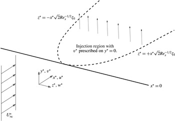
An analogue of the classical boundary layer adjacent to a flat plate, with leading edge at $x^{\ast }=0$ and subject to fluid injection at the surface. The classical ‘blow off’ results (Kassoy Reference Kassoy1970, Reference Kassoy1971, Reference Kassoy1974) are independent of $z^{\ast }$ , whereas here we force three-dimensionality directly by injection through a (narrow, symmetric) slot of spanwise (half-) width $\sqrt{2}x^{\ast }Re_{x}^{-1/2}\unicode[STIX]{x1D701}_{0}$ , in the large $Re_{x}$ limit. Of particular interest is the wide slot limit $\unicode[STIX]{x1D701}_{0}\gg 1$ .

2 Formulation

To formulate the problem we assume that the flow adjacent to the plate is laminar, steady and incompressible, and is to be described according to a dimensional Cartesian coordinate system ( $x^{\ast },y^{\ast },z^{\ast }$ ), as shown in figure 1. We will retain the notation of the introduction, with a free-stream speed of $U_{\infty }^{\ast }$ and kinematic viscosity $\unicode[STIX]{x1D708}^{\ast }$ . The plate is defined by $y^{\ast }=0$ , $x^{\ast }\geqslant 0$ , and $x^{\ast }$ is increasing in the streamwise direction with a corresponding local Reynolds number $Re_{x}=x^{\ast }U_{\infty }^{\ast }/\unicode[STIX]{x1D708}^{\ast }\gg 1$ . A non-dimensional solution is sought in a rescaled coordinate system

(2.1a )

$$\begin{eqnarray}\displaystyle (z^{\ast },y^{\ast })=\sqrt{2}x^{\ast }Re_{x}^{-1/2}(\unicode[STIX]{x1D701},\unicode[STIX]{x1D702}). & & \displaystyle\end{eqnarray}$$

This $\unicode[STIX]{x1D701}$ scale is central to the formulation and allows for spanwise scales that are comparable to the boundary-layer thickness. For the velocity field, we introduce

(2.1b )

$$\begin{eqnarray}\displaystyle & \displaystyle u^{\ast }=U_{\infty }^{\ast }U(\unicode[STIX]{x1D701},\unicode[STIX]{x1D702})+\cdots \,, & \displaystyle\end{eqnarray}$$

(2.1c )

$$\begin{eqnarray}\displaystyle & \displaystyle (v^{\ast },w^{\ast })=U_{\infty }^{\ast }Re_{x}^{-1/2}(V(\unicode[STIX]{x1D701},\unicode[STIX]{x1D702})+\cdots \,,W(\unicode[STIX]{x1D701},\unicode[STIX]{x1D702})+\cdots \,), & \displaystyle\end{eqnarray}$$

whilst the dimensional pressure field is

(2.1d )

$$\begin{eqnarray}\displaystyle p^{\ast }=\unicode[STIX]{x1D70C}^{\ast }{U_{\infty }^{\ast }}^{2}(Re_{x}^{-1/2}p+Re_{x}^{-1}P(\unicode[STIX]{x1D701},\unicode[STIX]{x1D702})+\cdots \,), & & \displaystyle\end{eqnarray}$$

where $\unicode[STIX]{x1D70C}^{\ast }$ is the constant fluid density. Here $p$ is the classical pressure correction obtained in the two-dimensional theory, but for these three-dimensional flows $P$ is the significant term, as it affects the leading-order solution.

In what follows attention is focused on transpiration through the plate surface of the form

(2.2)

$$\begin{eqnarray}\displaystyle v^{\ast }(\unicode[STIX]{x1D701},\unicode[STIX]{x1D702}=0)=U_{\infty }^{\ast }Re_{x}^{-1/2}V_{transp}(\unicode[STIX]{x1D701}). & & \displaystyle\end{eqnarray}$$

This is not a conceptual restriction of this formulation and more general $x^{\ast }$ dependencies can be handled by parabolic marching/development in the downstream direction. The advantage of the choice (2.2) lies in a self-similar development with $x^{\ast }$ , leaving us to only solve in the cross-sectional plane spanned by $\unicode[STIX]{x1D701}$ and $\unicode[STIX]{x1D702}$ .

Applying a boundary-layer approximation, under the assumption that the local Reynolds number $Re_{x}\gg 1$ , results in a system that retains viscous diffusion in the cross-sectional (that is, constant $x^{\ast }$ ) plane and the spanwise/transverse momentum equations are both affected by the pressure term $P$ . It is preferable to cross-differentiate and eliminate this pressure term, then employ a slight change of the dependent variables via

(2.3a )

$$\begin{eqnarray}\displaystyle & \displaystyle V(\unicode[STIX]{x1D701},\unicode[STIX]{x1D702})={\textstyle \frac{1}{\sqrt{2}}}(\unicode[STIX]{x1D702}U(\unicode[STIX]{x1D701},\unicode[STIX]{x1D702})-\unicode[STIX]{x1D6F7}(\unicode[STIX]{x1D701},\unicode[STIX]{x1D702})), & \displaystyle\end{eqnarray}$$

(2.3b )

$$\begin{eqnarray}\displaystyle & \displaystyle W(\unicode[STIX]{x1D701},\unicode[STIX]{x1D702})={\textstyle \frac{1}{\sqrt{2}}}(\unicode[STIX]{x1D701}U(\unicode[STIX]{x1D701},\unicode[STIX]{x1D702})-\unicode[STIX]{x1D6F9}(\unicode[STIX]{x1D701},\unicode[STIX]{x1D702})); & \displaystyle\end{eqnarray}$$

this leaves

$\unicode[STIX]{x1D6F7}$ and

$\unicode[STIX]{x1D6F9}$ as the variables of interest. This slight reformulation is equivalent to that found in (for example) Stewartson (1954) for the two-dimensional Falkner–Skan problem or Pal & Rubin (1971) for three-dimensional flow along a corner.

The above formulation results in the boundary-region equations in the form:

(2.4a )

$$\begin{eqnarray}\displaystyle & \displaystyle 2U=\unicode[STIX]{x1D6F7}_{\unicode[STIX]{x1D702}}+\unicode[STIX]{x1D6F9}_{\unicode[STIX]{x1D701}}, & \displaystyle\end{eqnarray}$$

(2.4b )

$$\begin{eqnarray}\displaystyle & \displaystyle \unicode[STIX]{x1D6E9}=\unicode[STIX]{x1D6F9}_{\unicode[STIX]{x1D702}}-\unicode[STIX]{x1D6F7}_{\unicode[STIX]{x1D701}}, & \displaystyle\end{eqnarray}$$

(2.4c )

$$\begin{eqnarray}\displaystyle & \displaystyle \unicode[STIX]{x1D6FB}^{2}U=-\unicode[STIX]{x1D6F7}U_{\unicode[STIX]{x1D702}}-\unicode[STIX]{x1D6F9}U_{\unicode[STIX]{x1D701}}, & \displaystyle\end{eqnarray}$$

(2.4d )

$$\begin{eqnarray}\displaystyle & \displaystyle \unicode[STIX]{x1D6FB}^{2}\unicode[STIX]{x1D6E9}=2[\unicode[STIX]{x1D701}UU_{\unicode[STIX]{x1D702}}-\unicode[STIX]{x1D702}UU_{\unicode[STIX]{x1D701}}]-\unicode[STIX]{x1D6F7}\unicode[STIX]{x1D6E9}_{\unicode[STIX]{x1D702}}-\unicode[STIX]{x1D6F9}\unicode[STIX]{x1D6E9}_{\unicode[STIX]{x1D701}}-2U\unicode[STIX]{x1D6E9}, & \displaystyle\end{eqnarray}$$

where

$\unicode[STIX]{x1D6FB}^{2}$ is the two-dimensional Laplacian in the plane spanned by

$\unicode[STIX]{x1D702}$ and

$\unicode[STIX]{x1D701}$ . Whilst perhaps less intuitive than the primitive variable formulation, this system is well known for its application to corner boundary-layer flows, see for example Pal & Rubin (1971). It is advantageous to use this formulation because (2.4a ) and (2.4b ) can be combined to give expressions for the Laplacian of

$\unicode[STIX]{x1D6F7}$ and

$\unicode[STIX]{x1D6F9}$ . This yields a system of the form

$\unicode[STIX]{x1D6FB}^{2}\text{}\underline{Q}=\text{}\underline{R}(\text{}\underline{Q},\unicode[STIX]{x1D701},\unicode[STIX]{x1D702})$ , where

$\text{}\underline{Q}=(U,\unicode[STIX]{x1D6F7},\unicode[STIX]{x1D6F9},\unicode[STIX]{x1D6E9})$ and

$\text{}\underline{R}$ is a nonlinear function of the unknowns and position in the plane. This approach allows for a relatively straightforward numerical discretisation scheme.

This system is to be solved subject to $U\rightarrow 1$ , $\unicode[STIX]{x1D6E9}\rightarrow 0$ , $\unicode[STIX]{x1D6F9}\rightarrow \unicode[STIX]{x1D701}$ as $\unicode[STIX]{x1D702}\rightarrow \infty$ , corresponding to a uniform external flow with no cross-flow. At $\unicode[STIX]{x1D701}=0$ we assume appropriate symmetry conditions whilst for large $\unicode[STIX]{x1D701}$ the solution is the usual flat-plate boundary layer. At the surface of the plate ( $\unicode[STIX]{x1D702}=0$ ), we require that $U=0$ , $\unicode[STIX]{x1D6F9}=0$ and surface transpiration (2.2) leads to

(2.5a )

$$\begin{eqnarray}\displaystyle \unicode[STIX]{x1D6F7}(\unicode[STIX]{x1D701},\unicode[STIX]{x1D702}=0)=-\sqrt{2}V_{transp}(\unicode[STIX]{x1D701}). & & \displaystyle\end{eqnarray}$$

We will focus on cases where the transpiration is largely uniform and exists over a finite-spanwise width, by taking

(2.5b )

$$\begin{eqnarray}\displaystyle V_{transp}(\unicode[STIX]{x1D701})=\frac{K}{2\sqrt{2}}(1-\tanh (\unicode[STIX]{x1D6FE}(|\unicode[STIX]{x1D701}/\unicode[STIX]{x1D701}_{0}|-1))). & & \displaystyle\end{eqnarray}$$

This gives an approximate top-hat shape to the transverse velocity profile at the plate surface, with $\unicode[STIX]{x1D701}_{0}$ defining the spanwise extent of the transpiration region on the $(2x^{\ast }\unicode[STIX]{x1D708}^{\ast }/U_{\infty }^{\ast })^{1/2}$ scale, $\unicode[STIX]{x1D6FE}$ defines the rapidity of the transition from transpiration to no transpiration (and is introduced largely for numerical expediency) and $K$ defines the magnitude of the transpiration.

Suction from the boundary layer is $K<0$ , whilst $K>0$ is injection into the layer. In what follows, we will take $\unicode[STIX]{x1D6FE}=20$ as a default parameter unless otherwise stated, and focus our attention on injection ( $K>0$ ) rather than the more straightforward suction case. We note that this parameterisation of the injection velocity is consistent with that employed in the two-dimensional problem, as discussed at some length in the works of Kassoy (Reference Kassoy1970, Reference Kassoy1971, Reference Kassoy1974) regarding ‘blow off’. It must be highlighted however that the dimensional transpiration velocity, when scaled according to (2.1), includes a multiplicative factor of $2^{-1/2}$ , being $U_{\infty }^{\ast }Re_{x}^{-1/2}K/\sqrt{2}$ .

2.1 Numerical implementation

One may be tempted to solve (2.4) under the assumption that the flow returns to the Blasius solution when sufficiently far from the injection region. Attempting this approach shows that the decay towards the Blasius state in the far field is in general algebraic and therefore requires very large domains. As a consequence, our numerical method seeks to reduce the size of the computational domain by imposing far-field boundary conditions that are consistent with the asymptotic decay towards the Blasius state in the far field.

We can explicitly remove the Blasius base flow by making the substitution

(2.6a )

$$\begin{eqnarray}\displaystyle & \displaystyle U(\unicode[STIX]{x1D701},\unicode[STIX]{x1D702})=U_{B}(\unicode[STIX]{x1D702})+\tilde{U} (\hat{\unicode[STIX]{x1D701}},\unicode[STIX]{x1D702}), & \displaystyle\end{eqnarray}$$

(2.6b )

$$\begin{eqnarray}\displaystyle & \displaystyle \unicode[STIX]{x1D6F7}(\unicode[STIX]{x1D701},\unicode[STIX]{x1D702})=\unicode[STIX]{x1D6F7}_{B}(\unicode[STIX]{x1D702})+\tilde{\unicode[STIX]{x1D6F7}}(\hat{\unicode[STIX]{x1D701}},\unicode[STIX]{x1D702}), & \displaystyle\end{eqnarray}$$

(2.6c )

$$\begin{eqnarray}\displaystyle & \displaystyle \unicode[STIX]{x1D6F9}(\unicode[STIX]{x1D701},\unicode[STIX]{x1D702})=\unicode[STIX]{x1D701}\unicode[STIX]{x1D6F9}_{B}(\unicode[STIX]{x1D702})+\unicode[STIX]{x1D701}_{0}\tilde{\unicode[STIX]{x1D6F9}}(\hat{\unicode[STIX]{x1D701}},\unicode[STIX]{x1D702}), & \displaystyle\end{eqnarray}$$

(2.6d )

$$\begin{eqnarray}\displaystyle & \displaystyle \unicode[STIX]{x1D6E9}(\unicode[STIX]{x1D701},\unicode[STIX]{x1D702})=\unicode[STIX]{x1D701}\unicode[STIX]{x1D6E9}_{B}(\unicode[STIX]{x1D702})+\unicode[STIX]{x1D701}_{0}\tilde{\unicode[STIX]{x1D6E9}}(\hat{\unicode[STIX]{x1D701}},\unicode[STIX]{x1D702}), & \displaystyle\end{eqnarray}$$

into the governing system (2.4). Here the tilde quantities represent a (nonlinear) perturbation that is driven purely by the presence of the injection slot and we employ the rescaled coordinate

$\hat{\unicode[STIX]{x1D701}}=\unicode[STIX]{x1D701}/\unicode[STIX]{x1D701}_{0}$ to span the extent of the slot. In the absence of injection, the tilde quantities are all zero, and the solution is simply

$U_{B}=\unicode[STIX]{x1D6F7}_{B}^{\prime }$ ,

$\unicode[STIX]{x1D6F9}_{B}=\unicode[STIX]{x1D6F7}_{B}^{\prime }$ ,

$\unicode[STIX]{x1D6E9}_{B}=\unicode[STIX]{x1D6F7}_{B}^{\prime \prime }$ , where (2.4) shows that

$\unicode[STIX]{x1D6F7}_{B}$ satisfies the Blasius equation

(2.7)

$$\begin{eqnarray}\displaystyle \unicode[STIX]{x1D6F7}_{B}^{\prime \prime \prime }+\unicode[STIX]{x1D6F7}_{B}\unicode[STIX]{x1D6F7}_{B}^{\prime \prime }=0, & & \displaystyle\end{eqnarray}$$

and the prime notation indicates differentiation with respect to $\unicode[STIX]{x1D702}$ .

The decomposition (2.6) allows the far-field behaviour of $(\tilde{U} ,\tilde{\unicode[STIX]{x1D6F7}},\tilde{\unicode[STIX]{x1D6F9}},\tilde{\unicode[STIX]{x1D6E9}})$ to be explicitly enforced as part of the numerical solution procedure. The far-field asymptotic behaviour is discussed in detail in Hewitt & Duck (Reference Hewitt and Duck2014) and we only present the main results here. It is sufficient here to note that for $\unicode[STIX]{x1D701}\gg 1$ and/or $\unicode[STIX]{x1D702}\gg 1$ , $\tilde{\unicode[STIX]{x1D6F7}}$ and $\tilde{\unicode[STIX]{x1D6F9}}$ both satisfy the harmonic equation, leading to

(2.8a,b )

$$\begin{eqnarray}\displaystyle \tilde{\unicode[STIX]{x1D6F7}}\sim \frac{A\unicode[STIX]{x1D702}}{\hat{\unicode[STIX]{x1D701}}^{2}+\unicode[STIX]{x1D702}^{2}},\quad \tilde{\unicode[STIX]{x1D6F9}}\sim \frac{A\hat{\unicode[STIX]{x1D701}}}{\hat{\unicode[STIX]{x1D701}}^{2}+\unicode[STIX]{x1D702}^{2}}, & & \displaystyle\end{eqnarray}$$

whilst $\tilde{U}$ and $\tilde{\unicode[STIX]{x1D6E9}}$ are both exponentially small. Here $A$ is a constant that must be determined as part of the global computation of (2.4) via the decomposition (2.6). If $A>0$ then the flow field has a net mass transport towards the centreline ( $\unicode[STIX]{x1D702}=\hat{\unicode[STIX]{x1D701}}=0$ ) in the far field, whilst $A<0$ corresponds to net outflow.

In classical boundary layers, algebraic decay into a free stream is typically not allowed. This conclusion is drawn from an examination of the properties of harmonic outer solutions, which would necessarily be singular at all points on approaching the boundary (e.g. Brown & Stewartson Reference Brown and Stewartson1965; Hewitt, Duck & Stow Reference Hewitt, Duck and Stow2002). However, these arguments do not apply to the three-dimensional solutions with short-spanwise scales discussed herein. In our case (2.8), the vorticity still decays exponentially and the outer Laplace problem is only singular along a line.

A second-order (finite-difference) method for the numerical solution of (2.4) subject to the decomposition (2.6) is employed; this follows the method of Hewitt & Duck (Reference Hewitt and Duck2014). The computational mesh is non-uniformly spaced in the $\hat{\unicode[STIX]{x1D701}},\unicode[STIX]{x1D702}$ plane to ensure that more nodes are concentrated near the plate surface, within the injection region ( $\hat{\unicode[STIX]{x1D701}}<1$ ) and at the edge of the injection region ( $\hat{\unicode[STIX]{x1D701}}=1$ ) where the injection velocity changes rapidly to zero. At each nodal point the four unknowns $(\tilde{U} ,\tilde{\unicode[STIX]{x1D6F7}},\tilde{\unicode[STIX]{x1D6F9}},\tilde{\unicode[STIX]{x1D6E9}})$ are stored. Newton iteration is used to determine the $4N_{\hat{\unicode[STIX]{x1D701}}}N_{\unicode[STIX]{x1D702}}+1$ unknowns, where $N_{\hat{\unicode[STIX]{x1D701}}}$ and $N_{\unicode[STIX]{x1D702}}$ are the number of nodes in the ( $\hat{\unicode[STIX]{x1D701}},\unicode[STIX]{x1D702}$ ) directions, and the additional unknown is the mass flux coefficient denoted by $A$ in (2.8). At each iteration, the linear system is sparse and the inversion is achieved by use of the MUMPS library (Amestoy, Duff & L’Excellent Reference Amestoy, Duff and L’Excellent2000); the number of degrees of freedom ranges up to approximately $5.76\times 10^{6}$ depending up the strength of the injection flow. In general, larger values of $K$ or $\unicode[STIX]{x1D701}_{0}$ require more degrees of freedom (larger $N_{\hat{\unicode[STIX]{x1D701}}}$ and $N_{\unicode[STIX]{x1D702}}$ ) and a larger computational domain. For example, for $K=2.5$ , $\unicode[STIX]{x1D701}_{0}=16$ our choices were $N_{\hat{\unicode[STIX]{x1D701}}}=N_{\unicode[STIX]{x1D702}}=1201$ with a domain truncation of $\hat{\unicode[STIX]{x1D701}}<20$ (i.e. $\unicode[STIX]{x1D701}<320$ ) and $\unicode[STIX]{x1D702}<320$ .

3 Results

In the absence of any injection through the plate surface ( $K=0$ ) the solution remains two-dimensional, and is provided by (2.7). Injection through the plate surface is only over a finite-spanwise length scale parameterised by $\unicode[STIX]{x1D701}_{0}$ , as described by (2.5), and therefore any non-zero $K$ will necessarily induce a three-dimensional response.

In the classical two-dimensional theory (Neiland et al. Reference Neiland, Bogolepov, Dudin and Lipatov2008, p. 173), increasing injection through the plate surface eventually leads to a detachment of the boundary layer. This detachment occurs at a critical $K\approx 0.876$ and is associated with a vanishing of the streamwise shear on the plate, and a shear layer that becomes infinitely displaced from the surface. Between this shear layer and the plate surface there is no substantial streamwise motion. It is therefore a natural question to address the relevance of this behaviour to our more general three-dimensional flow when $\unicode[STIX]{x1D701}_{0}\gg 1$ . That is, to what extent (if any) do we recover the two-dimensional classical results for injection over increasing slot widths, and is $K\approx 0.876$ still a critical injection speed at which the boundary layer detaches entirely from the surface?

3.1 Increasing injection slot width

On solving (2.4) subject to injection at the plate surface, $K>0$ , we find that the flow can be characterised as one of three types, as the injection slot width $\unicode[STIX]{x1D701}_{0}$ increases. In the remainder of this section we will discuss the differences between these three types of flow response with an emphasis on their physical features, then in § 4 we will describe these regimes asymptotically for $\unicode[STIX]{x1D701}_{0}\gg 1$ .

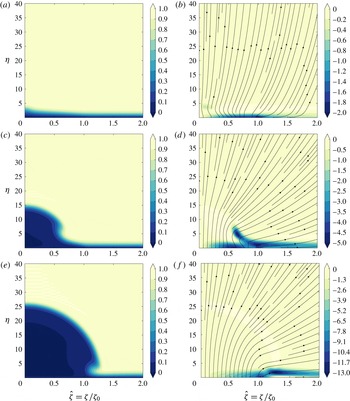
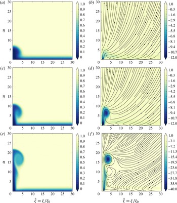
In figure 2 the flow is shown for three values of the injection amplitude $K=0.5,1.5,2.5$ and a fixed slot width of $\unicode[STIX]{x1D701}_{0}=20$ . For this relatively large value of $\unicode[STIX]{x1D701}_{0}$ these three injection amplitudes show three distinct types of behaviour. In what follows we classify these three types of response and identify the critical injection amplitudes associated with each type.

Figure 2.

The three flow regimes observed for $K>0$ (blowing) into an otherwise two-dimensional boundary layer; only $\unicode[STIX]{x1D701}>0$ is shown here with assumed symmetry about $\unicode[STIX]{x1D701}=0$ . Results are shown for a wall transpiration (2.5), with $\unicode[STIX]{x1D701}_{0}=20$ , $\unicode[STIX]{x1D6FE}=20$ and (a,b) $K=0.5$ (c,d) $K=1.5$ and (e,f) $K=2.5$ . The left-hand column shows contours of streamwise velocity $U$ , whilst the right-hand column shows the perturbation vorticity component $\unicode[STIX]{x1D701}_{0}\tilde{\unicode[STIX]{x1D6E9}}$ from (2.6) together with the corresponding particle path lines in the $\unicode[STIX]{x1D701}$ – $\unicode[STIX]{x1D702}$ plane.

3.1.1 Type I: weak injection ( $0<K<K_{I}$ )

The streamwise shear evaluated at the plate surface remains non-zero in this regime, ranging from the Blasius value far away from the injection slot ( $\hat{\unicode[STIX]{x1D701}}\gg 1$ ) to a minimum at the centreline of the injection region ( $\hat{\unicode[STIX]{x1D701}}=0$ ). There is a slight thickening of the boundary layer on approaching $\hat{\unicode[STIX]{x1D701}}=0$ , but otherwise the injection flow does not dominate the response. This is seen in figure 2(a,b), for $K=0.5$ and $\unicode[STIX]{x1D701}_{0}=20$ , which shows (a) the streamwise velocity $U$ and (b) the (scaled perturbation) vorticity $\tilde{\unicode[STIX]{x1D6E9}}$ ; both of these quantities are only influenced in the near-wall region.

The effects of wall transpiration in this case are mostly confined to the thin region of vorticity adjacent to the plate surface, where $\unicode[STIX]{x1D702}=O(1)$ . This level of blowing is not sufficient to push the layer away from the plate surface, but it does lead to a slow variation of the layer’s properties over the long ( $\unicode[STIX]{x1D701}_{0}\gg 1$ ) length scale. Any blowing-induced increase in the thickness of this layer near the plate means a reduction of the streamwise mass flux, and this deficit must be compensated for by an increase in the mass transferred to the bulk flow via $V$ and $W$ , as defined by (2.3). This displacement induced flow is in addition to the extra mass contributed by the blowing through the plate surface. In terms of the computational formulation, this means that as $K$ increases, so must the magnitude of $A$ , as defined by (2.8).

This flow response is obtained for $0<K<K_{I}$ , and we demonstrate in § 4.1 below that $K_{I}\approx 0.876$ , i.e. the same critical injection rate at which the two-dimensional solution is ‘blown off’. At injection rates larger than $K_{I}$ we move instead to a moderate injection regime in which the effects of blowing become more prominent.

3.1.2 Type II: moderate injection ( $K_{I}<K<K_{II}$ )

At values of the transpiration amplitude greater than $K_{I}$ but less than a further critical value, which we label $K_{II}$ the flow response in the injection region ( $\hat{\unicode[STIX]{x1D701}}<1$ ) changes. In the classical two-dimensional problem, there are no solutions for this rate of injection. However, for the boundary-region equations, a solution is obtained, albeit with very low shear at the plate surface near $\unicode[STIX]{x1D701}=0$ .

In this regime there is a vorticity component $\tilde{\unicode[STIX]{x1D6E9}}$ , which is displaced away from the plate boundary ( $\unicode[STIX]{x1D702}=0$ ) and near $\hat{\unicode[STIX]{x1D701}}=0$ a low-speed streak develops, within which $U\approx 0$ . These features can be seen in figure 2(c,d), where the low-speed streak is visible in (c), with an associated displacement of vorticity away from the wall in (d). For the type I solutions described above, the slight thickening of the layer near to $\hat{\unicode[STIX]{x1D701}}=0$ does not grow as the injection slot width $\unicode[STIX]{x1D701}_{0}$ is increased. However, in this type II regime, a widening slot width leads to an increasingly prominent low-speed streak. The presence of this low-speed region leads to a reduction in the streamwise mass flux, which is compensated for by an increased radial flow into the far field, as described by (2.8).

The low streamwise speeds within the streak are separated from the higher-speed outer flow by a displaced shear layer, which appears to have approximately constant curvature near to the centreline ( $\hat{\unicode[STIX]{x1D701}}=0$ ). The asymptotic theory presented below in § 4.2 points to $K_{II}\approx 1.95$ , with the exact value determined in terms of the precise spanwise form of the injection profile.

3.1.3 Type III: strong injection ( $K>K_{II}$ )

At sufficiently large injection amplitudes $K>K_{II}$ , increasing the width of the injection slot results in an even more prominent low-speed streak. An example of this regime is shown in figure 2(e,f) where a dominant large low-speed streak is observed that is in fact wider than the injection slot width (which ends at $\unicode[STIX]{x1D701}/\unicode[STIX]{x1D701}_{0}\approx 1$ ). The low-speed region appears to be circular, with a radius of $O(\unicode[STIX]{x1D701}_{0})$ ; we confirm this scaling in a subsequent asymptotic description below. A shear layer delineates the edge of this low-speed streak. Below this shear layer the streamwise velocity is small ( $U\approx 0$ ), whilst above it free-stream conditions are found with $U\approx 1$ . There is a non-zero vorticity perturbation associated with the shear layer, but it is not visible on the contour scale shown in figure 2(f).

In the absence of streamwise motion inside the streak, any mass transfer across the plate surface must exit via the surrounding shear layer. As we will demonstrate in § 4.2, we are able to provide a solution for the mass transfer through the shear layer as a function of its radius. By matching this mass flux through the shear layer (out of the streak) to that entering the streak via the injection slot, we can predict the streak radius.

4 Asymptotic descriptions for wide injection slots

Below we present asymptotic descriptions (guided by the numerical results of the previous section) for each of the three nonlinear flow states for increasing injection slot widths ( $\unicode[STIX]{x1D701}_{0}\gg 1$ ). In this discussion we address weak and strong injection first, leaving the (more complex) intermediate moderate injection case for last.

4.1 Type I: weak injection ( $K<K_{I}$ )

Despite the presence of injection, a viscous layer persists across the injection slot width, leading to an inner region that is spanned by $\unicode[STIX]{x1D702}=O(1)$ and $\unicode[STIX]{x1D701}=O(\unicode[STIX]{x1D701}_{0})$ , where $\unicode[STIX]{x1D701}_{0}$ is the lateral extent of the injection region defined by (2.5). To leading order this layer has no cross-flow. To describe this region we again use $\hat{\unicode[STIX]{x1D701}}=\unicode[STIX]{x1D701}/\unicode[STIX]{x1D701}_{0}$ , together with

(4.1a,b )

$$\begin{eqnarray}\displaystyle U(\unicode[STIX]{x1D701},\unicode[STIX]{x1D702};\unicode[STIX]{x1D701}_{0})=U_{0}(\hat{\unicode[STIX]{x1D701}},\unicode[STIX]{x1D702})+\cdots \,,\quad \unicode[STIX]{x1D6F7}(\unicode[STIX]{x1D701},\unicode[STIX]{x1D702};\unicode[STIX]{x1D701}_{0})=\unicode[STIX]{x1D6F7}_{0}(\hat{\unicode[STIX]{x1D701}},\unicode[STIX]{x1D702})+\cdots \,, & & \displaystyle\end{eqnarray}$$

(4.1c,d )

$$\begin{eqnarray}\displaystyle \unicode[STIX]{x1D6F9}(\unicode[STIX]{x1D701},\unicode[STIX]{x1D702};\unicode[STIX]{x1D701}_{0})=\unicode[STIX]{x1D701}_{0}\hat{\unicode[STIX]{x1D701}}\unicode[STIX]{x1D6F9}_{0}(\hat{\unicode[STIX]{x1D701}},\unicode[STIX]{x1D702})+\cdots \,,\quad \unicode[STIX]{x1D6E9}(\unicode[STIX]{x1D701},\unicode[STIX]{x1D702};\unicode[STIX]{x1D701}_{0})=\unicode[STIX]{x1D701}_{0}\hat{\unicode[STIX]{x1D701}}\unicode[STIX]{x1D6E9}_{0}(\hat{\unicode[STIX]{x1D701}},\unicode[STIX]{x1D702})+\cdots \,. & & \displaystyle\end{eqnarray}$$

In the absence of any cross-flow $W\approx 0$ , as defined by (2.3), a solution exists in the form

(4.2)

$$\begin{eqnarray}\displaystyle (U_{0},\unicode[STIX]{x1D6F7}_{0},\unicode[STIX]{x1D6F9}_{0},\unicode[STIX]{x1D6E9}_{0})=(U_{I},\unicode[STIX]{x1D6F7}_{I},U_{I},{U_{I}}_{\unicode[STIX]{x1D702}}), & & \displaystyle\end{eqnarray}$$

for which (2.4) reduces at leading order to

(4.3a )

$$\begin{eqnarray}\displaystyle & \displaystyle U_{I}={\unicode[STIX]{x1D6F7}_{I}}_{\unicode[STIX]{x1D702}}+\hat{\unicode[STIX]{x1D701}}{U_{I}}_{\hat{\unicode[STIX]{x1D701}}}, & \displaystyle\end{eqnarray}$$

(4.3b )

$$\begin{eqnarray}\displaystyle & \displaystyle {U_{I}}_{\unicode[STIX]{x1D702}\unicode[STIX]{x1D702}}=-\unicode[STIX]{x1D6F7}_{I}{U_{I}}_{\unicode[STIX]{x1D702}}-\hat{\unicode[STIX]{x1D701}}U_{I}{U_{I}}_{\hat{\unicode[STIX]{x1D701}}}. & \displaystyle\end{eqnarray}$$

$U_{I}>0$ for all

$\unicode[STIX]{x1D702}>0$ this solution can be extended from

$\hat{\unicode[STIX]{x1D701}}\gg 1$ towards

$\hat{\unicode[STIX]{x1D701}}=0$ by parabolic marching, subject to the conditions

(4.3c,d )

$$\begin{eqnarray}\displaystyle U_{I}=0,\quad \unicode[STIX]{x1D6F7}_{I}=\unicode[STIX]{x1D6F7}_{transp},\quad \text{on }\unicode[STIX]{x1D702}=0, & & \displaystyle\end{eqnarray}$$

(4.3e )

$$\begin{eqnarray}\displaystyle U_{I}\rightarrow 1,\quad \text{as }\unicode[STIX]{x1D702}\rightarrow \infty , & & \displaystyle\end{eqnarray}$$

where the surface transpiration $\unicode[STIX]{x1D6F7}_{transp}$ is defined implicitly by (2.5). The starting state for $\hat{\unicode[STIX]{x1D701}}\gg 1$ is simply the Blasius solution.

Figure 3.

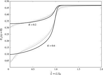
The shear distribution along the plate $U_{\unicode[STIX]{x1D702}}(\unicode[STIX]{x1D702}=0,\hat{\unicode[STIX]{x1D701}})$ for $\unicode[STIX]{x1D701}_{0}=20$ (dashed) and $\unicode[STIX]{x1D701}_{0}=40$ (solid) for $K=0.2$ and $K=0.6$ , as determined by solution of (2.4). For comparison the shear distribution predicted by the parabolic system (4.3), shown as the thicker line.

Figure 3 shows the shear distribution along the plate, for solutions of the ‘full’ system (2.4) with injection profiles given by (2.5) where $\unicode[STIX]{x1D6FE}=20$ , $\unicode[STIX]{x1D701}_{0}=20,40$ and $K=0.2,0.6$ . For comparison, the leading order $\unicode[STIX]{x1D701}_{0}\gg 1$ prediction provided by parabolically marching (4.3) is also shown. The full numerical data are consistent with and approaching the $\unicode[STIX]{x1D701}_{0}\gg 1$ prediction, apart from within a decreasing inner region around $\hat{\unicode[STIX]{x1D701}}=0$ . We will address this $\hat{\unicode[STIX]{x1D701}}\ll 1$ behaviour separately in appendix A, where there is firm evidence that three-dimensional eigensolutions play a role in this region.

In general, the parabolic solution terminates at $\hat{\unicode[STIX]{x1D701}}=0$ with a solution that is consistent with the classical two-dimensional states described in § 1, which only exist for $K\lesssim 0.876$ . Marching of (4.3) for $K\gtrsim 0.876$ leads to a singular response at a finite value of $\hat{\unicode[STIX]{x1D701}}$ , associated with a zero of $U_{0\unicode[STIX]{x1D702}}(\unicode[STIX]{x1D702}=0)$ .

For $\unicode[STIX]{x1D702}\gg 1$ , away from the parabolic layer, the far-field conditions provide

(4.4)

$$\begin{eqnarray}\displaystyle \unicode[STIX]{x1D6F7}_{0}\sim \unicode[STIX]{x1D702}+\unicode[STIX]{x1D6FF}_{B}+\unicode[STIX]{x1D6FF}_{transp}(\hat{\unicode[STIX]{x1D701}}), & & \displaystyle\end{eqnarray}$$

which is a statement regarding the vertical velocity induced in the outer flow due to the presence of the parabolic layer. Here $\unicode[STIX]{x1D6FF}_{B}$ is the displacement associated with the classical Blasius solution in the absence of transpiration (it is approximately $-1.2$ ). The imposition of a wall transpiration over a finite-spanwise region also induces a spanwise varying displacement that we denoted above as $\unicode[STIX]{x1D6FF}_{transp}(\hat{\unicode[STIX]{x1D701}})$ . If $K=0$ then the tilde quantities in (2.6) are zero and $\unicode[STIX]{x1D6FF}_{transp}=0$ , but for general values of $K$ , $\unicode[STIX]{x1D6FF}_{transp}\neq 0$ and is determined by spanwise marching of the parabolic-layer equations.

We now consider an outer inviscid region spanned by $\unicode[STIX]{x1D702}=\unicode[STIX]{x1D701}_{0}\hat{\unicode[STIX]{x1D702}}$ and $\unicode[STIX]{x1D701}=\unicode[STIX]{x1D701}_{0}\hat{\unicode[STIX]{x1D701}}$ ; this is an outer region of the boundary-region equations (2.4), and as such is $O(x^{\ast }Re_{x}^{-1/2}\unicode[STIX]{x1D701}_{0})$ on the dimensional transverse and spanwise scales. In this region, we can look for the perturbation to an underlying Blasius state

(4.5)

$$\begin{eqnarray}\displaystyle \unicode[STIX]{x1D6F7}=\unicode[STIX]{x1D701}_{0}\hat{\unicode[STIX]{x1D702}}+\unicode[STIX]{x1D6FF}_{B}+\unicode[STIX]{x1D719}(\hat{\unicode[STIX]{x1D701}},\hat{\unicode[STIX]{x1D702}}), & & \displaystyle\end{eqnarray}$$

where $\unicode[STIX]{x1D719}=O(1)$ in order to match with the $\unicode[STIX]{x1D6FF}_{transp}(\hat{\unicode[STIX]{x1D701}})$ induced by the parabolic solution and $\unicode[STIX]{x1D701}_{0}\hat{\unicode[STIX]{x1D702}}+\unicode[STIX]{x1D6FF}_{B}$ is simply the outer limit of the Blasius solution. Numerical evidence from the full solution suggests that both $U$ and $\unicode[STIX]{x1D6E9}$ remain $o(\unicode[STIX]{x1D701}_{0}^{-2})$ , which leaves a harmonic problem for $\unicode[STIX]{x1D719}$ ,

(4.6)

$$\begin{eqnarray}\hat{\unicode[STIX]{x1D6FB}}^{2}\unicode[STIX]{x1D719}=0,\end{eqnarray}$$

subject to

(4.7)

$$\begin{eqnarray}\displaystyle \unicode[STIX]{x1D719}(\hat{\unicode[STIX]{x1D701}},\hat{\unicode[STIX]{x1D702}}=0)=\unicode[STIX]{x1D6FF}_{transp}(\hat{\unicode[STIX]{x1D701}}). & & \displaystyle\end{eqnarray}$$

This is effectively determining the outer flow from the vertical mass transport induced in the parabolic layer by the presence of the surface transpiration.

The solution to the outer problem can now be given via a standard Green’s function approach

(4.8)

$$\begin{eqnarray}\unicode[STIX]{x1D719}(\hat{\unicode[STIX]{x1D701}},\hat{\unicode[STIX]{x1D702}})=\frac{1}{\unicode[STIX]{x03C0}}\int _{z=-\infty }^{+\infty }\frac{\unicode[STIX]{x1D6FF}_{transp}(z)\hat{\unicode[STIX]{x1D702}}}{\hat{\unicode[STIX]{x1D702}}^{2}+(\hat{\unicode[STIX]{x1D701}}-z)^{2}}\,\text{d}z.\end{eqnarray}$$

In the far field we know from (2.8) that

(4.9)

$$\begin{eqnarray}\displaystyle \unicode[STIX]{x1D719}\sim \frac{A\unicode[STIX]{x1D702}}{\unicode[STIX]{x1D701}^{2}+\unicode[STIX]{x1D702}^{2}}=\frac{\hat{A}\hat{\unicode[STIX]{x1D702}}}{\hat{\unicode[STIX]{x1D701}}^{2}+\hat{\unicode[STIX]{x1D702}}^{2}}, & & \displaystyle\end{eqnarray}$$

where $A=\unicode[STIX]{x1D701}_{0}\hat{A}$ ; similar expressions are possible for the far-field contribution to the $\unicode[STIX]{x1D6F9}$ component. Given this far-field behaviour, the total radial mass flux (or more strictly because this is in the plane, an area flux) due to spanwise variation at infinity is $A\unicode[STIX]{x03C0}$ , whereas the flux from the parabolic layer induced by the surface injection is $M\unicode[STIX]{x1D701}_{0}$ , where

(4.10a )

$$\begin{eqnarray}\displaystyle M=\int _{-\infty }^{\infty }\unicode[STIX]{x1D6FF}_{transp}(\hat{\unicode[STIX]{x1D701}})\,\text{d}\hat{\unicode[STIX]{x1D701}}. & & \displaystyle\end{eqnarray}$$

Mass conservation therefore allows us to predict the coefficient $A$ in (2.8) must be

(4.10b )

$$\begin{eqnarray}\displaystyle A=\frac{M}{\unicode[STIX]{x03C0}}\unicode[STIX]{x1D701}_{0}. & & \displaystyle\end{eqnarray}$$

Figure 4.

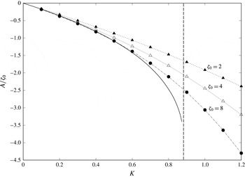
Numerically determined values (data points) of $A/\unicode[STIX]{x1D701}_{0}$ for increasing injection velocities $K$ . Shown as a solid line is the asymptotic prediction, $M/\unicode[STIX]{x03C0}$ , as determined from (4.10a ). The vertical line shows the critical value $K=K_{I}\approx 0.876$ .

In figure 4 we show a comparison of the numerically computed values of $A$ with the asymptotic prediction provided by (4.10). For this comparison we perform the parabolic marching of (4.3), from an initial state of a Blasius profile, to determine $\unicode[STIX]{x1D6FF}_{transp}$ via (4.4). This allows for computation of the transverse mass flux induced by this viscous response via the integral definition of $M$ in (4.10a ). Excellent agreement with the asymptotic description is found (confirming the linear dependency of $A$ on $\unicode[STIX]{x1D701}_{0}$ ), but the approach fails at $K=K_{I}\approx 0.876$ . It is also clear that the singular response of the parabolic solution associated with a reversal of the cross-flow at the critical injection rate of $K\approx 0.876$ is strongly mitigated by finite- $\unicode[STIX]{x1D701}_{0}$ effects.

4.2 Type III: strong injection ( $K>K_{II}$ )

In this regime there is a sizeable low-speed streak associated with injection velocities larger than a critical value of $K_{II}$ ; this value is determined as part of the asymptotic description as $\unicode[STIX]{x1D701}_{0}\rightarrow \infty$ given below. The flow field in this regime shares the qualitative features of figure 2(e,f), with the spatial extent of the streak becoming large as the injection slot width ( $\unicode[STIX]{x1D701}_{0}$ ) is increased.

We seek to capture the details of this streak using the coordinates $\hat{\unicode[STIX]{x1D702}}=\unicode[STIX]{x1D702}/\unicode[STIX]{x1D701}_{0}$ and $\hat{\unicode[STIX]{x1D701}}=\unicode[STIX]{x1D701}/\unicode[STIX]{x1D701}_{0}$ , and the numerical evidence of § 3 suggests the following scalings:

(4.11a,b )

$$\begin{eqnarray}\displaystyle U(\unicode[STIX]{x1D701},\unicode[STIX]{x1D702};\unicode[STIX]{x1D701}_{0})=o(\unicode[STIX]{x1D701}_{0}^{-1})+\cdots \,,\quad \unicode[STIX]{x1D6F7}(\unicode[STIX]{x1D701},\unicode[STIX]{x1D702};\unicode[STIX]{x1D701}_{0})=\unicode[STIX]{x1D6F7}^{\ast }(\hat{\unicode[STIX]{x1D701}},\hat{\unicode[STIX]{x1D702}})+\cdots \,, & & \displaystyle\end{eqnarray}$$

(4.11c,d )

$$\begin{eqnarray}\displaystyle \unicode[STIX]{x1D6F9}(\unicode[STIX]{x1D701},\unicode[STIX]{x1D702};\unicode[STIX]{x1D701}_{0})=\unicode[STIX]{x1D6F9}^{\ast }(\hat{\unicode[STIX]{x1D701}},\hat{\unicode[STIX]{x1D702}})+\cdots \,,\quad \unicode[STIX]{x1D6E9}(\unicode[STIX]{x1D701},\unicode[STIX]{x1D702};\unicode[STIX]{x1D701}_{0})=\unicode[STIX]{x1D701}_{0}^{-1}\unicode[STIX]{x1D6E9}^{\ast }(\hat{\unicode[STIX]{x1D701}},\hat{\unicode[STIX]{x1D702}})+\cdots \,. & & \displaystyle\end{eqnarray}$$

This leads to the following leading-order system within the streak:

(4.12a )

$$\begin{eqnarray}\displaystyle & \displaystyle \unicode[STIX]{x1D6F7}_{\hat{\unicode[STIX]{x1D702}}}^{\ast }=-\unicode[STIX]{x1D6F9}_{\hat{\unicode[STIX]{x1D701}}}^{\ast }, & \displaystyle\end{eqnarray}$$

(4.12b )

$$\begin{eqnarray}\displaystyle & \displaystyle \unicode[STIX]{x1D6E9}^{\ast }=\unicode[STIX]{x1D6F9}_{\hat{\unicode[STIX]{x1D702}}}^{\ast }-\unicode[STIX]{x1D6F7}_{\hat{\unicode[STIX]{x1D701}}}^{\ast }, & \displaystyle\end{eqnarray}$$

(4.12c )

$$\begin{eqnarray}\displaystyle & \displaystyle \unicode[STIX]{x1D6F7}^{\ast }\unicode[STIX]{x1D6E9}_{\hat{\unicode[STIX]{x1D702}}}^{\ast }+\unicode[STIX]{x1D6F9}^{\ast }\unicode[STIX]{x1D6E9}_{\hat{\unicode[STIX]{x1D701}}}^{\ast }=0. & \displaystyle\end{eqnarray}$$

We can usefully re-pose this problem in terms of a streamfunction

(4.13)

$$\begin{eqnarray}G(\unicode[STIX]{x1D701},\unicode[STIX]{x1D702})=\unicode[STIX]{x1D701}_{0}G^{\ast }(\hat{\unicode[STIX]{x1D701}},\hat{\unicode[STIX]{x1D702}})+\cdots \,,\end{eqnarray}$$

such that

(4.14)

$$\begin{eqnarray}\unicode[STIX]{x1D6F9}^{\ast }=-G_{\hat{\unicode[STIX]{x1D702}}}^{\ast },\quad \unicode[STIX]{x1D6F7}^{\ast }=G_{\hat{\unicode[STIX]{x1D701}}}^{\ast }.\end{eqnarray}$$

This leads to the usual Poisson formulation for a two-dimensional, inviscid, but rotational, incompressible flow, where $\unicode[STIX]{x1D6E9}^{\ast }$ is the vorticity. Using (2.3), $U\approx 0$ implies that (to leading order) $W=G_{\hat{\unicode[STIX]{x1D702}}}^{\ast }/\sqrt{2}$ is the spanwise velocity, whilst $V=-G_{\hat{\unicode[STIX]{x1D701}}}^{\ast }/\sqrt{2}$ is the transverse velocity.

At the boundary, $G^{\ast }(\hat{\unicode[STIX]{x1D701}},\hat{\unicode[STIX]{x1D702}}=0)=G_{w}^{\ast }(\hat{\unicode[STIX]{x1D701}})$ , where $G_{w}^{\ast }$ effectively defines the scaled mass flux (in the plane, per unit distance downstream) through the injection slot, via

(4.15)

$$\begin{eqnarray}\displaystyle G_{w}^{\ast }(\hat{\unicode[STIX]{x1D701}})=-\sqrt{2}\int _{0}^{\hat{\unicode[STIX]{x1D701}}}V_{transp}\,\text{d}\hat{\unicode[STIX]{x1D701}}. & & \displaystyle\end{eqnarray}$$

The streak exists within a large semi-circular region, of radius $r=(\unicode[STIX]{x1D702}^{2}+\unicode[STIX]{x1D701}^{2})^{1/2}=r_{s}$ ; in terms of the scaled coordinates, this becomes $\hat{r}=(\hat{\unicode[STIX]{x1D702}}^{2}+\hat{\unicode[STIX]{x1D701}}^{2})^{1/2}=\hat{r}_{s}$ , where $r_{s}=\unicode[STIX]{x1D701}_{0}\hat{r}_{s}$ . Outside of the streak region (and of the circular shear layer discussed below) the response is irrotational with $U\equiv 1$ and $\unicode[STIX]{x1D6E9}\equiv 0$ (to leading order), along with

(4.16a,b )

$$\begin{eqnarray}\displaystyle \unicode[STIX]{x1D6F7}=\unicode[STIX]{x1D701}_{0}\hat{\unicode[STIX]{x1D702}}+\frac{A\hat{\unicode[STIX]{x1D702}}}{\unicode[STIX]{x1D701}_{0}(\hat{\unicode[STIX]{x1D702}}^{2}+\hat{\unicode[STIX]{x1D701}}^{2})}+O(\unicode[STIX]{x1D701}_{0}^{-2}),\quad \unicode[STIX]{x1D6F9}=\unicode[STIX]{x1D701}_{0}\hat{\unicode[STIX]{x1D701}}+\frac{A\hat{\unicode[STIX]{x1D701}}}{\unicode[STIX]{x1D701}_{0}(\hat{\unicode[STIX]{x1D702}}^{2}+\hat{\unicode[STIX]{x1D701}}^{2})}+O(\unicode[STIX]{x1D701}_{0}^{-2}), & & \displaystyle\end{eqnarray}$$

which describe the underlying far-field (uniform flow) solution, plus the algebraic decay (with amplitude $A$ ) of the induced three-dimensional response. In order to match with the solution inside the streak, we must have that both $\unicode[STIX]{x1D6F7}$ and $\unicode[STIX]{x1D6F9}$ are $o(\unicode[STIX]{x1D701}_{0})$ , which leads to

(4.17)

$$\begin{eqnarray}\displaystyle A=-\unicode[STIX]{x1D701}_{0}^{2}\hat{r}_{s}^{2}. & & \displaystyle\end{eqnarray}$$

This partially confirms the semi-circular shape of the streak, although we still require the connecting solution through the shear layer.

In the shear layer at the edge of the streak, we employ a new radial coordinate $R=r-r_{s}$ , and angle $\unicode[STIX]{x1D703}$ , measured from the plate. Assuming all flow quantities are $O(1)$ in this region, we obtain

(4.18a )

$$\begin{eqnarray}\displaystyle & \displaystyle 2U=\unicode[STIX]{x1D6F7}_{R}\sin \unicode[STIX]{x1D703}+\unicode[STIX]{x1D6F9}_{R}\cos \unicode[STIX]{x1D703}, & \displaystyle\end{eqnarray}$$

(4.18b )

$$\begin{eqnarray}\displaystyle & \displaystyle \unicode[STIX]{x1D6E9}=\unicode[STIX]{x1D6F9}_{R}\sin \unicode[STIX]{x1D703}-\unicode[STIX]{x1D6F7}_{R}\cos \unicode[STIX]{x1D703}, & \displaystyle\end{eqnarray}$$

(4.18c )

$$\begin{eqnarray}\displaystyle & \displaystyle U_{RR}=-\unicode[STIX]{x1D6F7}U_{R}\sin \unicode[STIX]{x1D703}-\unicode[STIX]{x1D6F9}U_{R}\cos \unicode[STIX]{x1D703}, & \displaystyle\end{eqnarray}$$

(4.18d )

$$\begin{eqnarray}\displaystyle & \displaystyle \unicode[STIX]{x1D6E9}_{RR}=-\unicode[STIX]{x1D6F7}\unicode[STIX]{x1D6E9}_{R}\sin \unicode[STIX]{x1D703}-\unicode[STIX]{x1D6F9}\unicode[STIX]{x1D6E9}_{R}\cos \unicode[STIX]{x1D703}-2\unicode[STIX]{x1D6E9}U. & \displaystyle\end{eqnarray}$$

The final equation would have contained two (solitary)

$O(\unicode[STIX]{x1D701}_{0})$ terms, but these cancel if the streak is semi-circular in form (confirming our earlier assertion). Boundary conditions for the semi-circular shear layer are

$U\rightarrow 0$ ,

$\unicode[STIX]{x1D6E9}\rightarrow 0$ as

$R\rightarrow -\infty$ , and

$U\rightarrow 1$ ,

$\unicode[STIX]{x1D6E9}\rightarrow 0$ along with

$\unicode[STIX]{x1D6F7}\rightarrow 2R\sin \unicode[STIX]{x1D703}$ and

$\unicode[STIX]{x1D6F9}\rightarrow 2R\cos \unicode[STIX]{x1D703}$ as

$R\rightarrow \infty$ .

On reformulating in terms of the radial flow contribution in the cross-sectional plane,

(4.19a )

$$\begin{eqnarray}\displaystyle F=\unicode[STIX]{x1D6F7}\sin \unicode[STIX]{x1D703}+\unicode[STIX]{x1D6F9}\cos \unicode[STIX]{x1D703}, & & \displaystyle\end{eqnarray}$$

we obtain

(4.19b )

$$\begin{eqnarray}\displaystyle F_{RRR}+FF_{RR}=0, & & \displaystyle\end{eqnarray}$$

to be solved subject to $F(0)=0$ (associated with an arbitrary $O(1)$ translation of the origin), $F^{\prime }(\infty )\rightarrow 2$ as $R\rightarrow \infty$ and $F^{\prime }(-\infty )\rightarrow 0$ as $R\rightarrow -\infty$ . This is equivalent to the standard planar mixing-layer solution, albeit in terms of a radial coordinate, see for example Schlichting & Gersten (Reference Schlichting and Gersten2003, p. 667). Numerical solution of this free shear layer indicates that $F(-\infty )\approx -1.238$ .

This leaves the vorticity term $\unicode[STIX]{x1D6E9}$ to be determined, together with the individual contributions of $\unicode[STIX]{x1D6F7}$ and $\unicode[STIX]{x1D6F9}$ to the now known $F$ . The $\unicode[STIX]{x1D6E9}$ equation is then

(4.19c )

$$\begin{eqnarray}\displaystyle \unicode[STIX]{x1D6E9}_{R}+F\unicode[STIX]{x1D6E9}=\text{const}. & & \displaystyle\end{eqnarray}$$

Evaluation in the far field shows the constant to be zero, and a solution is therefore

(4.19d )

$$\begin{eqnarray}\displaystyle \unicode[STIX]{x1D6E9}=C_{1}F_{RR}, & & \displaystyle\end{eqnarray}$$

where $C_{1}$ is a constant.

The function $F$ is the radial velocity contribution from $\unicode[STIX]{x1D6F7}$ and $\unicode[STIX]{x1D6F9}$ (albeit with $F<0$ corresponding to radial outflow). In terms of the (scaled) streamfunction describing the flow inside the streak, this same radial component is

(4.20)

$$\begin{eqnarray}\displaystyle \frac{1}{\hat{r}}\frac{\unicode[STIX]{x2202}G^{\ast }}{\unicode[STIX]{x2202}\unicode[STIX]{x1D703}}. & & \displaystyle\end{eqnarray}$$

Matching with the radial flow through the shear layer, the solution in the streak requires the condition

(4.21)

$$\begin{eqnarray}\displaystyle \left.\frac{1}{\hat{r}_{s}}\frac{\unicode[STIX]{x2202}G^{\ast }}{\unicode[STIX]{x2202}\unicode[STIX]{x1D703}}\right|_{\hat{r}=\hat{r}_{s}}=-F(-\infty ), & & \displaystyle\end{eqnarray}$$

or, as $F(-\infty )$ is independent of $\unicode[STIX]{x1D703}$ :

(4.22)

$$\begin{eqnarray}\displaystyle G^{\ast }|_{\hat{r}=\hat{r}_{s}}=\text{const.}-\hat{r}_{s}F(-\infty )\unicode[STIX]{x1D703}. & & \displaystyle\end{eqnarray}$$

For a symmetric injection with no mass flux across the centreline $\hat{\unicode[STIX]{x1D701}}=0$ ( $\unicode[STIX]{x1D703}=\unicode[STIX]{x03C0}/2$ )

(4.23)

$$\begin{eqnarray}\displaystyle G^{\ast }(\hat{r}_{s},\unicode[STIX]{x1D703})=-\hat{r}_{s}F(-\infty )(\unicode[STIX]{x1D703}-\unicode[STIX]{x03C0}/2). & & \displaystyle\end{eqnarray}$$

Evaluation on the plate ( $\unicode[STIX]{x1D703}=0$ ) and requiring that the mass flux through the injection slot matches with that through the shear layer at the outer extent of the streak, requires

(4.24)

$$\begin{eqnarray}\displaystyle \hat{r}_{s}F(-\infty )\frac{\unicode[STIX]{x03C0}}{2}=G_{w}^{\ast }(\hat{\unicode[STIX]{x1D701}}=\hat{r}_{s}). & & \displaystyle\end{eqnarray}$$

Failure of this condition would mean a discontinuity in the streamfunction at $O(\unicode[STIX]{x1D701}_{0})$ as the semi-circular shear layer connects with the plate boundary layer.

The constraint (4.24) is a condition for the (scaled) radius of the streak, $\hat{r}_{s}$ . For sufficiently large values of $\unicode[STIX]{x1D6FE}$ , (2.5b ) is well approximated by $-K\hat{\unicode[STIX]{x1D701}}/\sqrt{2}$ for $\hat{\unicode[STIX]{x1D701}}<1$ and $-K/\sqrt{2}$ for $\hat{\unicode[STIX]{x1D701}}\geqslant 1$ . Hence (4.15) yields $G_{w}^{\ast }(\hat{\unicode[STIX]{x1D701}}=\hat{r}_{s})\approx -K$ , on assuming that $\hat{r}_{s}>1$ , leaving

(4.25a )

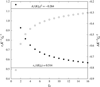
$$\begin{eqnarray}\displaystyle r_{s}=\unicode[STIX]{x1D701}_{0}\hat{r}_{s}=-\frac{2K\unicode[STIX]{x1D701}_{0}}{\unicode[STIX]{x03C0}F(-\infty )}\approx 0.514K\unicode[STIX]{x1D701}_{0}. & & \displaystyle\end{eqnarray}$$

Hence (4.17) provides

(4.25b )

$$\begin{eqnarray}\displaystyle A\sim -\frac{4K^{2}\unicode[STIX]{x1D701}_{0}^{2}}{\unicode[STIX]{x03C0}^{2}F(-\infty )^{2}}\approx -0.264K^{2}\unicode[STIX]{x1D701}_{0}^{2}. & & \displaystyle\end{eqnarray}$$

Figure 5.

Numerically determined values of $A$ (open circles and right-hand scale) and $r_{s}$ (solid circles and left-hand scale) in the strong injection regime (with $K=2.5>K_{II}$ ) as the injection slot width $\unicode[STIX]{x1D701}_{0}$ increases. These numerical results are rescaled according to the leading-order asymptotic behaviour, and compared with the $\unicode[STIX]{x1D701}_{0}\gg 1$ predictions of (4.25); as shown by the solid lines.

This argument only applies if $\hat{r}_{s}>1$ . If $\hat{r}_{s}<1$ , then $G_{w}^{\ast }(\hat{\unicode[STIX]{x1D701}}=\hat{r}_{s})\approx -K\hat{r}_{s}$ , in which case the radius of the streak is eliminated from the mass flux constraint (4.24), and the condition cannot (in general) be satisfied. So $\hat{r}_{s}=r_{s}/\unicode[STIX]{x1D701}_{0}=1$ serves to identify the critical injection velocity ( $K_{II}$ ) for the development of this flow regime. Setting $\hat{r}_{s}=1$ and $K=K_{II}$ in (4.25a ) provides

(4.26)

$$\begin{eqnarray}\displaystyle K_{II}=-\frac{\unicode[STIX]{x03C0}F(-\infty )}{2}\approx 1.95. & & \displaystyle\end{eqnarray}$$

In figure 5 we show the predicted unscaled streak radius ( $r_{s}$ ) and far-field constant $A$ for increasing widths of the injection slot ( $\unicode[STIX]{x1D701}_{0}$ ) with a fixed injection velocity $K>K_{II}$ . The agreement is clear, although there is evidence of a higher-order $O(1)$ contribution to both $r_{s}$ and $A$ that we have made no attempt to determine asymptotically. For this comparison we have chosen to measure the streak radius by determining the value of $r_{s}$ such that $U(\unicode[STIX]{x1D701}=0,\unicode[STIX]{x1D702}=r_{s})=0.5$ , being the mid-way value between the $U\approx 0$ in the streak and $U\approx 1$ in the far field. As a final point, it is worth noting that the large magnitude of $A=O(\unicode[STIX]{x1D701}_{0}^{2})$ in this regime makes calculations challenging, in particular the imposition of the conditions (2.8) is crucial. As $A$ increases, a larger computational domain is required to accurately reproduce the leading-order (algebraic) asymptotic behaviour in the far field. For figure 5 (for example), we use a domain of size $\hat{\unicode[STIX]{x1D701}}<20$ , $\unicode[STIX]{x1D702}<320$ with $1201\times 1201$ nodes for $\unicode[STIX]{x1D701}_{0}=16$ . Less challenging parameter values can be resolved with smaller domains and fewer nodes.

4.3 Type II: moderate injection ( $K_{I}<K<K_{II}$ )

This regime provides a transition between states of type I and III, and is therefore expected to share some of the characteristics of both, but as a consequence has a rather more complex structure, leading to a less complete asymptotic (global) description.

Figure 6.

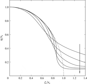
Contours of $U=0.5$ in the rescaled coordinate system $(\unicode[STIX]{x1D701}/r_{s},\unicode[STIX]{x1D702}/r_{s})$ , where $r_{s}$ is chosen such that $U(\unicode[STIX]{x1D701}=0,\unicode[STIX]{x1D702}=r_{s})=0.5$ ; shown here for $\unicode[STIX]{x1D701}_{0}=10$ and $K=1,1.2,1.4,1.6,1.8$ increasing in the direction of the arrow shown. The dashed line is the predicted circular shear-layer location for the type III solutions that exist for $K>1.95$ and large $\unicode[STIX]{x1D701}_{0}$ .

The dominant feature at moderate injection velocities is a low-speed streak, as in the strong injection regime, but in this case the streak is not semi-circular. Numerical evidence, as shown in figure 2(c) suggests that the streak’s edge is approximately circular only over a finite range of angle rather than extending all the way to the plate boundary. The shear layer deviates from being circular at an angle that is dependent on the injection rate $K$ . Figure 6 shows the contour $U(\unicode[STIX]{x1D701},\unicode[STIX]{x1D702})=0.5$ (as a reasonable proxy for the shear-layer location that bounds the low-speed streak) for an injection slot width of $\unicode[STIX]{x1D701}_{0}=10$ and injection rates of $K=1,1.2,\ldots ,1.8$ . As can be seen from the figure, as $K$ is increased towards the critical value of $K_{II}\approx 1.95$ the circular portion of the shear layer increases until it approximates the quarter circle predicted in the leading-order asymptotic description of the type III regime.

Figure 7.

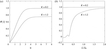
Values of $\unicode[STIX]{x1D6F9}/\unicode[STIX]{x1D701}$ measured in the injection region for $\unicode[STIX]{x1D701}_{0}=40$ and $K=0.2$ (type I) and $K=1.2$ (type II). In regions where $U\approx 1$ , $\unicode[STIX]{x1D6F9}/\unicode[STIX]{x1D701}\approx 1$ corresponds to no cross-flow velocity, with $W\approx 0$ as defined by (2.3). (a) Two profiles of $\unicode[STIX]{x1D6F9}/\unicode[STIX]{x1D701}$ are presented at $\unicode[STIX]{x1D701}=0.7\unicode[STIX]{x1D701}_{0}$ , for $K=0.2,1.2$ showing an attached layer at the plate in both cases. (b) The spanwise variation of $\unicode[STIX]{x1D6F9}/\unicode[STIX]{x1D701}$ is shown at $\unicode[STIX]{x1D702}=8$ , showing weak cross-flow velocity for $K=0.2$ but a non-trivial external cross-flow for $K=1.2$ .

In this type II regime, the size of the streak is smaller than the width of the injection region (that is, $r_{s}<\unicode[STIX]{x1D701}_{0}$ ). Outside of the streak but still near to the plate, the flow has the characteristics of an attached $\unicode[STIX]{x1D702}=O(1)$ viscous layer similar to that found in the type I states, as described by (4.3). An example profile of $\unicode[STIX]{x1D6F9}$ in this layer adjacent to the plate (but outside the streak) is shown in figure 7(a) at $\unicode[STIX]{x1D701}=0.7\unicode[STIX]{x1D701}_{0}$ (with $\unicode[STIX]{x1D701}_{0}=40$ ) for $K=1.2$ (type II) and for comparison we also show $K=0.2$ (type I). Away from the injection region, ( $\unicode[STIX]{x1D701}\gg \unicode[STIX]{x1D701}_{0}$ ) the solution in this layer decays to the Blasius state, but how this layer connects to the displaced shear layer in the injection region ( $\unicode[STIX]{x1D701}<\unicode[STIX]{x1D701}_{0}$ ) is non-trivial.

As noted in our discussion of the type I states, the parabolic on-plate layer (4.3) when marched in the spanwise coordinate to the centreline $\unicode[STIX]{x1D701}=0$ recovers the classical two-dimensional results described in § 1. Therefore when $K>K_{I}$ (as is the case in this type II regime) there is no such terminating solution at $\unicode[STIX]{x1D701}=0$ and (4.3) breaks down with a singularity in displacement thickness at a finite spanwise location. It is tempting to assume that the displaced shear layer and the layer adjacent to the plate connect via this steady separation, but there is little evidence to support this view in the full numerical results. Furthermore, the solution of (4.3) assumes that the far-field ( $\unicode[STIX]{x1D702}\gg 1$ ) condition is $\unicode[STIX]{x1D6F9}_{0}\rightarrow 1$ , which is the condition for no cross-flow at $O(\unicode[STIX]{x1D701}_{0})$ above this layer. This is true for type I solutions, but the displacement associated with the streak makes this assumption invalid in type II states.

Figure 7(a) shows the profile for $\unicode[STIX]{x1D6F9}(\unicode[STIX]{x1D701}=0.7\unicode[STIX]{x1D701}_{0},\unicode[STIX]{x1D702})/\unicode[STIX]{x1D701}$ (which is $\unicode[STIX]{x1D6F9}_{0}(\hat{\unicode[STIX]{x1D701}}=0.7,\unicode[STIX]{x1D702})$ in (4.3) to leading order) for $\unicode[STIX]{x1D701}_{0}=40$ and $K=0.2,1.2$ . For $K=0.2$ , the far-field value is approximately unity as expected for this type I state, whereas there is clearly a significant difference from unity for the type II state of $K=1.2$ . In both cases $U\approx 1$ away from the plate, so this deviation of $\unicode[STIX]{x1D6F9}/\unicode[STIX]{x1D701}$ from unity is indicative of the importance of cross-flow at the edge of this layer in the type II regime. This is also confirmed in figure 7(b), which shows $\unicode[STIX]{x1D6F9}/\unicode[STIX]{x1D701}$ at a fixed value of $\unicode[STIX]{x1D702}=8$ .

A solution to the parabolic problem (4.3) is therefore still relevant to the region outside the streak but adjacent to the plate in this case, but a more general external condition of $\unicode[STIX]{x1D6F9}_{0}\rightarrow \unicode[STIX]{x1D6F9}_{\infty }(\hat{\unicode[STIX]{x1D701}})$ is more appropriate (rather than $\unicode[STIX]{x1D6F9}_{0}\rightarrow 1$ as applied for type I solutions). This distribution of cross-flow velocity, $\unicode[STIX]{x1D6F9}_{\infty }$ , will be a function of the streak size and shape. Similarly the streak size and shape will be undetermined until the mass flux into it from the parabolic layer can be determined. Combining these observations suggests that an interactive approach (albeit within the confines of the boundary-region equations) is required, which couples all three regions (the viscous layer on the plate, the streak and the region outside both) together at leading order; this in itself would be a challenging computation.

5 Discussion

We have presented three-dimensional self-similar solutions to the ‘boundary-region equations’. These solutions correspond to injection through a slot of dimensional width $\unicode[STIX]{x1D701}_{0}(2x^{\ast }\unicode[STIX]{x1D708}^{\ast }/U_{\infty }^{\ast })^{1/2}$ and dimensional injection velocity $K(U_{\infty }^{\ast }\unicode[STIX]{x1D708}^{\ast }/x^{\ast })^{1/2}$ , where $x^{\ast }$ is the distance from the leading edge of a flat plate, placed in a fluid of vanishing kinematic viscosity $\unicode[STIX]{x1D708}^{\ast }$ with a free-stream speed of $U_{\infty }^{\ast }$ . Outside the injection slot the plate is treated as impermeable, and we thus recover the classical injection-free solutions near the plate in the far field. This choice of spatial dependence for the injection velocity and the slot width allows for solutions that are self-similar in the downstream coordinate. A more general downstream variations could be tackled in a similar manner, by parabolic marching in the downstream direction.

For the two-dimensional case it is known that the self-similar states cease to exist for $K\gtrsim 0.876$ , at which point the boundary layer is ‘blown off’ the plate surface. To continue these two-dimensional states beyond this value requires an interacting formulation outside the traditional boundary-layer equations. However, in the context of the boundary-region equations considered herein, solutions continue to exist with no evidence of a critical ‘blow off’ event.

When the width of the injection slot ( $\unicode[STIX]{x1D701}_{0}$ ) becomes large, three distinct flow regimes develop delineated by the magnitude of the blowing. The main (global) features of these three regimes have been described asymptotically, with good quantitative agreement for the bulk flow features. If the blowing parameter $K\lesssim 0.876$ then in the injection region we recover a three-dimensional analogue of the corresponding classical two-dimensional state. This state can be determined by parabolic marching from the far field in the spanwise direction into the injection region. However, even on approaching the centreline of the injection slot we typically do not fully recover the quantitative results of the classical approach, owing to a spatial instability (discussed in appendix A), which dominates close to the centreline.

At larger values of the injection parameter, $K$ , solutions develop a low-speed streak at the centreline of the injection region. For increasing $K$ the size of the streak increases, until for $K\gtrsim 1.95$ the streak becomes semi-circular and of a radius that is greater than the width of the injection slot. In this regime the streak is of dimensional radius $0.514K\unicode[STIX]{x1D701}_{0}(2x^{\ast }\unicode[STIX]{x1D708}^{\ast }/U_{\infty }^{\ast })^{1/2}$ .

The asymptotic descriptions of the low-speed streak that we have provided are robust to changes in the details of the injection profile, in the sense that any different choice for (2.5) could be approached in the same manner. In physical terms, the asymptotic development for large injection widths is dominated by the role of mass flux through the plate and a requirement for this to be balanced by the flux across the shear layer that bounds the streak. For example, the type III states balance the influx (into the streak) of $K\unicode[STIX]{x1D701}_{0}$ with the outflux of $F(-\infty )\unicode[STIX]{x03C0}r_{s}/2$ , where $F(-\infty )$ is the (constant) transpiration rate into the shear layer, (4.19b ), and $\unicode[STIX]{x03C0}r_{s}/2$ is simply the outer circumference of the streak (in the quarter plane $\unicode[STIX]{x1D702},\unicode[STIX]{x1D701}>0$ ). This condition determines the streak radius $r_{s}$ , as described by (4.25a ). A change of the injection profile from (2.5) to something more complicated would not alter this argument. For example, an alternative transpiration profile with zero mean flux may be considered, with injection of magnitude $K$ for $\unicode[STIX]{x1D701}\in [0,\unicode[STIX]{x1D701}_{0}]$ then suction of the same magnitude for $\unicode[STIX]{x1D701}\in [\unicode[STIX]{x1D701}_{0},2\unicode[STIX]{x1D701}_{0}]$ . The same asymptotic argument applies with little change and predicts that the streak radius is now $r_{s}=4K\unicode[STIX]{x1D701}_{0}/(F(-\infty )\unicode[STIX]{x03C0}+2K)$ . Note that in this case, the rescaled radius $\hat{r}_{s}=r_{s}/\unicode[STIX]{x1D701}_{0}$ no longer increases without bound for increasing $K$ and instead becomes saturated at $\hat{r}_{s}=2$ ; that is, the streak size becomes bounded by the end of the suction region.

The recent work of van Dommelen & Yapalparvi (Reference van Dommelen and Yapalparvi2014) examined two-dimensional boundary layers influenced by weak curvature. They showed that a Goldstein singularity (Goldstein Reference Goldstein1948) could be regularised by the inclusion of a spanwise-periodic blowing region. Key to their work was the inclusion of short-scale spanwise effects, motivated by the experimental use of microjets, and achieved through a curvature affected version of the boundary-region equations. Wall curvature ensured that the blowing region induced a (Görtler) vortex, which in some cases can persist downstream to the location at which separation would be found in the absence of blowing. The imposition of spanwise periodicity is important in the separation context of van Dommelen & Yapalparvi (Reference van Dommelen and Yapalparvi2014), because allowing the flow to return to being two-dimensional in the far field ( $\unicode[STIX]{x1D701}\gg 1$ ) will recover the singularity in that region. Furthermore in the presence of spanwise diffusion, a singularity in the far field means that parabolic marching must terminate at all spanwise locations. Our focus is the self-similar ‘blow off’ singularity rather than inhibiting separation. We have therefore removed the requirement for curvature, addressed a uniform external flow (Blasius), extended the blowing region to be at all streamwise locations, and relaxed the spanwise-periodic nature of the blowing to being an isolated region. Nevertheless, our results support those of van Dommelen & Yapalparvi (Reference van Dommelen and Yapalparvi2014) because they too remain unseparated, in the sense that there is no singularity.

Figure 8.

The behaviour for large injection velocities (increasing $K$ ) over a fixed slot (half-)width that is comparable to the two-dimensional Blasius boundary-layer thickness. Results are shown for a wall transpiration (2.5), with $\unicode[STIX]{x1D701}_{0}=1$ , $\unicode[STIX]{x1D6FE}=20$ and (a,b) $K=8$ (c,d) $K=16$ and (e,f) $K=32$ . The left-hand column shows contours of streamwise velocity $U$ , whilst the right-hand column shows the perturbation vorticity component $\unicode[STIX]{x1D701}_{0}\tilde{\unicode[STIX]{x1D6E9}}$ from (2.6) together with the corresponding particle path lines in the $\unicode[STIX]{x1D701}$ - $\unicode[STIX]{x1D702}$ plane. As specified in the key, only a subrange is displayed for contours of $\tilde{\unicode[STIX]{x1D6E9}}$ , to avoid the large contribution from the edge of the injection slot at $\hat{\unicode[STIX]{x1D701}}=1$ , $\unicode[STIX]{x1D702}=0$ .

The classical ‘blow off’ problem is only loosely related to the steady separation found in the analogous streamwise-developing problem, see for example Catherall et al. (Reference Catherall, Stewartson and Williams1965), but our results show that short-scale spanwise diffusion can remove the singularity present in the two-dimensional approach. Our results show significant regions of virtually stagnant streamwise flow; such states were found to have very low values of wall shear for both large spanwise-width blowing regions and large blowing rates. In this regard, we conclude by noting that more complex streak-like structures are possible for strong blowing at fixed injection widths. In figure 8 we repeat the measures employed in figure 2, but this time for fixed modest injection width $\unicode[STIX]{x1D701}_{0}=1$ and increasing injection amplitude $K=8,16,32$ , for the pairs of figures (a,b), (c,d) and (e,f) respectively. In the classical literature this is the ‘massive blowing’ or ‘blow hard’ (Cole & Aroesty Reference Cole and Aroesty1968) limit, and again we see no evidence of a critical ‘blow off’, but rather a streak that is largely of $O(1)$ (in the $\unicode[STIX]{x1D701}$ -scale) width and of increasing length in the transverse direction ( $\unicode[STIX]{x1D702}$ ). The exception is the uppermost portion of the streak, which is associated with a strong and localised patch of vorticity, as measured by the contours of the perturbation vorticity term $\tilde{\unicode[STIX]{x1D6E9}}$ . We have made no attempt at providing an asymptotic description for $K\gg 1$ , but numerical results suggest that the height of the streak increases approximately linearly with $K$ whilst there is some evidence of a slow growth in the size of the vorticity patch at the top of the streak. Again there is no evidence of (streamwise) flow reversal and increased blowing appears to be related directly to very small (but still positive) shear at the base of the streak.

Appendix A. The role of spatial eigenmodes for $\hat{\unicode[STIX]{x1D701}}\ll 1$

Figure 3 shows a comparison of the (streamwise) shear distributions on the plate for $\unicode[STIX]{x1D701}_{0}=20,40$ and $K=0.2,0.6<K_{I}$ , which is in the weak injection regime. For increasing $\unicode[STIX]{x1D701}_{0}$ there is good quantitative evidence of an approach to the leading-order ( $\unicode[STIX]{x1D701}_{0}\gg 1$ ) asymptotic theory provided by the parabolic layer (4.3). But there remains a marked deviation away from the predicted behaviour for small values of $\hat{\unicode[STIX]{x1D701}}$ . This feature can be observed in figure 3 as a rapid drop in the wall shear values for $\hat{\unicode[STIX]{x1D701}}\lesssim 0.2$ when compared to the asymptotic prediction.

The physical origin of this behaviour can be clarified by allowing for the spatial development of a weak cross-flow on approaching the centreline ( $\hat{\unicode[STIX]{x1D701}}=0$ ). To achieve this we again look for a solution to (2.4) in the form of (4.1). In § 4.1 we sought solutions with no cross-flow, which required $U_{0}=\unicode[STIX]{x1D6F9}_{0}$ and $\unicode[STIX]{x1D6E9}_{0}={U_{0}}_{\unicode[STIX]{x1D702}}$ in (4.1). However, here we consider the spatial development of a weak cross-flow, of $O(\unicode[STIX]{x1D716})$ say, by modifying (4.2) as follows:

(A 1)

$$\begin{eqnarray}\displaystyle & \displaystyle U_{0}=U_{I}(\hat{\unicode[STIX]{x1D701}},\unicode[STIX]{x1D702})+\unicode[STIX]{x1D716}u(\hat{\unicode[STIX]{x1D701}},\unicode[STIX]{x1D702}), & \displaystyle\end{eqnarray}$$

(A 2)

$$\begin{eqnarray}\displaystyle & \displaystyle \unicode[STIX]{x1D6F7}_{0}=\unicode[STIX]{x1D6F7}_{I}(\hat{\unicode[STIX]{x1D701}},\unicode[STIX]{x1D702})+\unicode[STIX]{x1D716}\unicode[STIX]{x1D711}(\hat{\unicode[STIX]{x1D701}},\unicode[STIX]{x1D702}), & \displaystyle\end{eqnarray}$$

(A 3)

$$\begin{eqnarray}\displaystyle & \displaystyle \unicode[STIX]{x1D6F9}_{0}=U_{I}(\hat{\unicode[STIX]{x1D701}},\unicode[STIX]{x1D702})+\unicode[STIX]{x1D716}\unicode[STIX]{x1D713}(\hat{\unicode[STIX]{x1D701}},\unicode[STIX]{x1D702}), & \displaystyle\end{eqnarray}$$

(A 4)

$$\begin{eqnarray}\displaystyle & \displaystyle \unicode[STIX]{x1D6E9}_{0}={U_{I}}_{\unicode[STIX]{x1D702}}(\hat{\unicode[STIX]{x1D701}},\unicode[STIX]{x1D702})+\unicode[STIX]{x1D716}\unicode[STIX]{x1D717}(\hat{\unicode[STIX]{x1D701}},\unicode[STIX]{x1D702}). & \displaystyle\end{eqnarray}$$

If $\unicode[STIX]{x1D716}=0$ , then we recover (4.3) and the solution of § 4.1, which has no cross-flow velocity. However, if $u\neq \unicode[STIX]{x1D713}$ the $O(\unicode[STIX]{x1D716})$ perturbations will in general have an associated cross-flow.

For $\unicode[STIX]{x1D716}\ll 1$ , a linearised system can be easily obtained for $(u,\unicode[STIX]{x1D711},\unicode[STIX]{x1D713},\unicode[STIX]{x1D717})$ , and for $\hat{\unicode[STIX]{x1D701}}\ll 1$ , solutions exist in the form

(A 5)

$$\begin{eqnarray}\displaystyle (u(\hat{\unicode[STIX]{x1D701}},\unicode[STIX]{x1D702}),\unicode[STIX]{x1D711}(\hat{\unicode[STIX]{x1D701}},\unicode[STIX]{x1D702}),\unicode[STIX]{x1D713}(\hat{\unicode[STIX]{x1D701}},\unicode[STIX]{x1D702}),\unicode[STIX]{x1D717}(\hat{\unicode[STIX]{x1D701}},\unicode[STIX]{x1D702}))=\hat{\unicode[STIX]{x1D701}}^{\unicode[STIX]{x1D706}}(u_{0}(\unicode[STIX]{x1D702}),\unicode[STIX]{x1D711}_{0}(\unicode[STIX]{x1D702}),\unicode[STIX]{x1D713}_{0}(\unicode[STIX]{x1D702}),\unicode[STIX]{x1D717}_{0}(\unicode[STIX]{x1D702})). & & \displaystyle\end{eqnarray}$$

This yields an eigenvalue problem for $\unicode[STIX]{x1D706}=\unicode[STIX]{x1D706}_{r}+i\unicode[STIX]{x1D706}_{i}$ , and clearly if $\unicode[STIX]{x1D706}_{r}<0$ we expect growth of this perturbation as $\hat{\unicode[STIX]{x1D701}}\rightarrow 0$ . In practice this growth is not unbounded, but its presence points to a need to reintroduce spanwise diffusive effects near to the centreline, even for large injection slot widths.

We have solved the eigenvalue problem for $\unicode[STIX]{x1D706}$ over a range of $K$ via a standard finite-difference formulation together with an application of the QZ algorithm. This shows that for $K\gtrsim -0.45$ , there is a single eigenvalue with $\unicode[STIX]{x1D706}_{r}<0$ , and the cross-flow-free solution obtained from (4.3) is susceptible to the growth of these modes in a relatively small region around the centreline $\hat{\unicode[STIX]{x1D701}}=0$ .

References

Amestoy, P. R., Duff, I. S. & L’Excellent, J.-Y. 2000 Multifrontal parallel distributed symmetric and unsymmetric solvers. Comput. Meth. Appl. Mech. Engng 184 (2), 501–520.Google Scholar

Brown, S. N. & Stewartson, K. 1965 On similarity solutions of the boundary-layer equations with algebraic decay. J. Fluid Mech. 23 (04), 673–687.Google Scholar

Catherall, D., Stewartson, K. & Williams, P. G. 1965 Viscous flow past a flat plate with uniform injection. Proc. R. Soc. Lond. A 284 (1398), 370–396.Google Scholar

Cole, J. D. & Aroesty, J. 1968 The blowhard problem inviscid flows with surface injection. Intl J. Heat Mass Transfer 11 (7), 1167–1183.Google Scholar

Dhanak, M. R. & Duck, P. W. 1997 The effects of freestream pressure gradient on a corner boundary layer. Proc. R. Soc. Lond. A 453 (1964), 1793–1815.Google Scholar

van Dommelen, L. L. & Yapalparvi, R. 2014 Laminar boundary-layer separation control by Görtler-scale blowing. Eur. J. Mech. (B/Fluids) 46, 1–16.Google Scholar

Elliott, L. 1968 Two-dimensional boundary layer theory with strong blowing. Q. J. Mech. Appl. Maths 21 (1), 77–91.Google Scholar

Emmons, H. W. & Leigh, D. C.1954 Tabulation of the Blasius function with blowing and suction ARC CP no. 157.Google Scholar

Fernandez, E., Kumar, R. & Alvi, F. 2013 Separation control on a low-pressure turbine blade using microjets. J. Propul. Power 29 (4), 867–881.Google Scholar

Goldstein, M. E., Sescu, A., Duck, P. W. & Choudhari, M. 2016 Nonlinear wakes behind a row of elongated roughness elements. J. Fluid Mech. 796, 516–557.CrossRef Google Scholar PubMed

Goldstein, R. J. 1971 Film cooling. Adv. Heat Transfer 7, 321–379.Google Scholar

Goldstein, S. 1948 On laminar boundary-layer flow near a position of separation. Q. J. Mech. Appl. Maths 1 (1), 43–69.CrossRef Google Scholar

Gross, J. F., Hartnett, J. P., Masson, D. J. & Gazley, C. 1961 A review of binary laminar boundary layer characteristics. Intl J. Heat Mass Transfer 3 (3), 198–221.CrossRef Google Scholar

Haidari, A. H. & Smith, C. R. 1994 The generation and regeneration of single hairpin vortices. J. Fluid Mech. 277, 135–162.CrossRef Google Scholar

Hewitt, R. E. & Duck, P. W. 2014 Three-dimensional boundary layers with short spanwise scales. J. Fluid Mech. 756, 452–469.Google Scholar

Hewitt, R. E., Duck, P. W. & Stow, S. R. 2002 Continua of states in boundary-layer flows. J. Fluid Mech. 468, 121–152.Google Scholar

Kassoy, D. R. 1970 On laminar boundary layer blowoff. SIAM J. Appl. Maths 18 (1), 29–40.Google Scholar

Kassoy, D. R. 1971 On laminar boundary-layer blow-off. Part 2. J. Fluid Mech. 48, 209–228.CrossRef Google Scholar

Kassoy, D. R. 1974 A resolution of the blow-off singularity for similarity flow on a flat plate. J. Fluid Mech. 62, 145–161.Google Scholar

Kemp, N. H.1951 The laminar three-dimensional boundary layer and a study of the flow past a side edge. M.Ae.S. thesis, Cornell University.Google Scholar

Klemp, J. B. & Acrivos, A. 1972 High Reynolds number flow past a flat plate with strong blowing. J. Fluid Mech. 51, 337–356.CrossRef Google Scholar

Liu, T. M. & Libby, P. A. 1971 Flame sheet model for stagnation point flows. Combust. Sci. Technol. 2 (5–6), 377–388.Google Scholar

Neiland, V. Ya., Bogolepov, V. V., Dudin, G. N. & Lipatov, I. I. 2008 Asymptotic Theory of Supersonic Viscous Gas Flows. Butterworth-Heinemann.Google Scholar

Pal, A. & Rubin, S. G. 1971 Asymptotic features of viscous flow along a corner. Q. Appl. Maths 29, 91–108.Google Scholar

Ricco, P. & Dilib, F. 2010 The influence of wall suction and blowing on boundary-layer laminar streaks generated by free-stream vortical disturbances. Phys. Fluids 22 (4), 044101.Google Scholar

Rosenhead, L. 1963 Laminar Boundary Layers. Clarendon.Google Scholar

Schlichting, H. & Gersten, K. 2003 Boundary-layer Theory. Springer.Google Scholar

Stewartson, K. 1954 Further solutions of the Falkner–Skan equation. Math. Proc. Camb. Phil. Soc. 50 (03), 454–465.Google Scholar

Watson, E. J. 1966 The equation of similar profiles in boundary-layer theory with strong blowing. Proc. R. Soc. Lond. A 294 (1437), 208–234.Google Scholar

Wundrow, D. W. & Goldstein, M. E. 2001 Effect on a laminar boundary layer of small-amplitude streamwise vorticity in the upstream flow. J. Fluid Mech. 426, 229–262.Google Scholar

Figure 1.An analogue of the classical boundary layer adjacent to a flat plate, with leading edge at $x^{\ast }=0$ and subject to fluid injection at the surface. The classical ‘blow off’ results (Kassoy 1970, 1971, 1974) are independent of $z^{\ast }$, whereas here we force three-dimensionality directly by injection through a (narrow, symmetric) slot of spanwise (half-) width $\sqrt{2}x^{\ast }Re_{x}^{-1/2}\unicode[STIX]{x1D701}_{0}$, in the large $Re_{x}$ limit. Of particular interest is the wide slot limit $\unicode[STIX]{x1D701}_{0}\gg 1$.

Figure 2.The three flow regimes observed for $K>0$ (blowing) into an otherwise two-dimensional boundary layer; only $\unicode[STIX]{x1D701}>0$ is shown here with assumed symmetry about $\unicode[STIX]{x1D701}=0$. Results are shown for a wall transpiration (2.5), with $\unicode[STIX]{x1D701}_{0}=20$, $\unicode[STIX]{x1D6FE}=20$ and (a,b) $K=0.5$ (c,d) $K=1.5$ and (e,f) $K=2.5$. The left-hand column shows contours of streamwise velocity $U$, whilst the right-hand column shows the perturbation vorticity component $\unicode[STIX]{x1D701}_{0}\tilde{\unicode[STIX]{x1D6E9}}$ from (2.6) together with the corresponding particle path lines in the $\unicode[STIX]{x1D701}$–$\unicode[STIX]{x1D702}$ plane.

Figure 3.The shear distribution along the plate $U_{\unicode[STIX]{x1D702}}(\unicode[STIX]{x1D702}=0,\hat{\unicode[STIX]{x1D701}})$ for $\unicode[STIX]{x1D701}_{0}=20$ (dashed) and $\unicode[STIX]{x1D701}_{0}=40$ (solid) for $K=0.2$ and $K=0.6$, as determined by solution of (2.4). For comparison the shear distribution predicted by the parabolic system (4.3), shown as the thicker line.

Figure 4.Numerically determined values (data points) of $A/\unicode[STIX]{x1D701}_{0}$ for increasing injection velocities $K$. Shown as a solid line is the asymptotic prediction, $M/\unicode[STIX]{x03C0}$, as determined from (4.10a). The vertical line shows the critical value $K=K_{I}\approx 0.876$.

Figure 5.Numerically determined values of $A$ (open circles and right-hand scale) and $r_{s}$ (solid circles and left-hand scale) in the strong injection regime (with $K=2.5>K_{II}$) as the injection slot width $\unicode[STIX]{x1D701}_{0}$ increases. These numerical results are rescaled according to the leading-order asymptotic behaviour, and compared with the $\unicode[STIX]{x1D701}_{0}\gg 1$ predictions of (4.25); as shown by the solid lines.

Figure 6.Contours of $U=0.5$ in the rescaled coordinate system $(\unicode[STIX]{x1D701}/r_{s},\unicode[STIX]{x1D702}/r_{s})$, where $r_{s}$ is chosen such that $U(\unicode[STIX]{x1D701}=0,\unicode[STIX]{x1D702}=r_{s})=0.5$; shown here for $\unicode[STIX]{x1D701}_{0}=10$ and $K=1,1.2,1.4,1.6,1.8$ increasing in the direction of the arrow shown. The dashed line is the predicted circular shear-layer location for the type III solutions that exist for $K>1.95$ and large $\unicode[STIX]{x1D701}_{0}$.

Figure 7.Values of $\unicode[STIX]{x1D6F9}/\unicode[STIX]{x1D701}$ measured in the injection region for $\unicode[STIX]{x1D701}_{0}=40$ and $K=0.2$ (type I) and $K=1.2$ (type II). In regions where $U\approx 1$, $\unicode[STIX]{x1D6F9}/\unicode[STIX]{x1D701}\approx 1$ corresponds to no cross-flow velocity, with $W\approx 0$ as defined by (2.3). (a) Two profiles of $\unicode[STIX]{x1D6F9}/\unicode[STIX]{x1D701}$ are presented at $\unicode[STIX]{x1D701}=0.7\unicode[STIX]{x1D701}_{0}$, for $K=0.2,1.2$ showing an attached layer at the plate in both cases. (b) The spanwise variation of $\unicode[STIX]{x1D6F9}/\unicode[STIX]{x1D701}$ is shown at $\unicode[STIX]{x1D702}=8$, showing weak cross-flow velocity for $K=0.2$ but a non-trivial external cross-flow for $K=1.2$.

Figure 8.The behaviour for large injection velocities (increasing $K$) over a fixed slot (half-)width that is comparable to the two-dimensional Blasius boundary-layer thickness. Results are shown for a wall transpiration (2.5), with $\unicode[STIX]{x1D701}_{0}=1$, $\unicode[STIX]{x1D6FE}=20$ and (a,b) $K=8$ (c,d) $K=16$ and (e,f) $K=32$. The left-hand column shows contours of streamwise velocity $U$, whilst the right-hand column shows the perturbation vorticity component $\unicode[STIX]{x1D701}_{0}\tilde{\unicode[STIX]{x1D6E9}}$ from (2.6) together with the corresponding particle path lines in the $\unicode[STIX]{x1D701}$-$\unicode[STIX]{x1D702}$ plane. As specified in the key, only a subrange is displayed for contours of $\tilde{\unicode[STIX]{x1D6E9}}$, to avoid the large contribution from the edge of the injection slot at $\hat{\unicode[STIX]{x1D701}}=1$, $\unicode[STIX]{x1D702}=0$.

Article contents

Injection into boundary layers: solutions beyond the classical form

Abstract

JFM classification

Information

1 Introduction

2 Formulation

2.1 Numerical implementation

3 Results

3.1 Increasing injection slot width

3.1.1 Type I: weak injection ( $0<K<K_{I}$ )

3.1.2 Type II: moderate injection ( $K_{I}<K<K_{II}$ )

3.1.3 Type III: strong injection ( $K>K_{II}$ )

4 Asymptotic descriptions for wide injection slots

4.1 Type I: weak injection ( $K<K_{I}$ )

4.2 Type III: strong injection ( $K>K_{II}$ )

4.3 Type II: moderate injection ( $K_{I}<K<K_{II}$ )

5 Discussion

Appendix A. The role of spatial eigenmodes for $\hat{\unicode[STIX]{x1D701}}\ll 1$

References

Save article to Kindle

Save article to Dropbox

Save article to Google Drive

Reply to: Submit a response

Your details

You have entered the maximum number of contributors

Conflicting interests