



1. Introduction
The similarity between the mathematical formulations of linear elasticity and slow viscous flow led Taylor (Reference Taylor1969) to suggest the fluid mechanical analogies of various classical problems from solid mechanics. Continuing in this vein, a number of studies have explored the buckling and folding of viscous sheets and the coiling and ‘sewing’ of liquid threads (Buckmaster, Nachman & Ting Reference Buckmaster, Nachman and Ting1975; Ribe Reference Ribe2002; Teichman & Mahadevan Reference Teichman and Mahadevan2003; Chiu-Webster & Lister Reference Chiu-Webster and Lister2006; Slim et al. Reference Slim, Balmforth, Craster and Miller2008; Ribe, Habibi & Bonn Reference Ribe, Habibi and Bonn2012; Slim, Teichman & Mahadevan Reference Slim, Teichman and Mahadevan2012). The implications of this work range from understanding the everyday observations of honey or syrup falling on toast, the manufacture of glass fibres and sheets, to inferences about the fate of subducting slabs in the Earth's mantle. In all these studies, the relatively thin geometry of the sheet or thread is exploited to derive reduced models describing the dynamics of the ‘viscida’, in analogy with the classical solid mechanics description of Euler's elastica (Love Reference Love1944).
Here, we pursue the analogy further, but consider the non-Newtonian version of the fluid mechanics problem, deriving reduced model equations for viscoelastic ribbons or sheets. We employ the Oldroyd-B model to describe the viscoelastic fluid (Bird, Armstrong & Hassager Reference Bird, Armstrong and Hassager1987), although the lack of substantial stretching in the configurations we consider means this particular choice for the constitutive law is relatively unimportant. We then use the reduced model to study the viscoelastic dynamics of some curling, bending and buckling problems. Our exploration follows on from a related study in which we examined the bending and stretching of sheets of yield-stress fluid (Balmforth & Hewitt Reference Balmforth and Hewitt2013), and we consider a similar suite of sample problems: ribbon curling, cantilevered and buckling beams, viscoelastic snap-through and the viscoelastic catenary.
The curling of ribbons has recently been rationalised in terms of the elasto-plastic deformation of a thin sheet of paper (Prior et al. Reference Prior, Moussou, Chakrabarti, Jensen and Juel2016): the drawing of a straight ribbon over a sharp edge induces an abrupt change in curvature that may plastically deform one side of the sheet whilst the other side deforms elastically, thereby imprinting the permanent deformation characterising the curled ribbon. However, any viscoelastic deformation of a thin sheet can accomplish the same task, as we illustrate here, and is familiar from the practicalities of curling hair (Barnes & Roberts Reference Barnes and Roberts2000; Zuidema et al. Reference Zuidema, Govaert, Baaijens, Ackermans and Asvadi2003). Other curling problems in which viscoelasticity likely plays a prominent role have been considered recently by Audoly, Callan-Jones & Brun (Reference Audoly, Callan-Jones and Brun2015), Tadrist, Brochard-Wyart & Cuvelier (Reference Tadrist, Brochard-Wyart and Cuvelier2012) and Arriagada, Massiera & Abkarian (Reference Arriagada, Massiera and Abkarian2014).
The exploration of the dynamics of elastica dates back to Galileo's cantilever, wherein an initially straight and clamped beam bends under gravity. Similarly, the buckling of elastic beams has a rich history. For a viscoelastic beam, one expects that the relaxation of the elastic stress introduces residual creep that prevents the beam from maintaining an elastically bent or buckled state. Instead, creep induces continued deformation beyond that state, or may even induce buckling below traditional elastic thresholds. In the solid mechanics literature, the latter is referred to as ‘creep buckling’ (Kempner Reference Kempner1954; Minahen & Knauss Reference Minahen and Knauss1993). Our reduced model for sheets of viscoelastic fluid captures such creep dynamics and is closely related to previous models for beams of viscoelastic solid. Unlike our current approach, however, the developments for viscoelastic solid beams do not typically begin with a reduction of the governing equations of solid mechanics with a constitutive law for the solid, but start from traditional ‘beam theory’. As such, curvatures are commonly taken to be small (whereas we take the curvature to be order one), and viscoelastic behaviour is incorporated using a general memory function. Our formulation takes a more fluid-mechanical approach: the Oldroyd-B model allows for long-term creep of the material and accounts for large deformations from the initially straight state.
In addition to the dynamics of creep buckling, the model can also be applied to study the analogue of elastic ‘snap-through’ instabilities. Here, a control parameter is used to march a structure through a bifurcation in which an elastic state is either lost or becomes unstable, precipitating a sudden transition to another state (e.g. Plaut & Virgin Reference Plaut and Virgin2009). Dissipation has been suggested to control the dynamics during snap-through in a number of problems (Gomez, Moulton & Vella Reference Gomez, Moulton and Vella2019), with biological applications ranging from the Venus fly trap (Forterre et al. Reference Forterre, Skotheim, Dumais and Mahadevan2005) to the snapping of the beak of a hummingbird or flagella of bacteria (Smith, Yanega & Ruina Reference Smith, Yanega and Ruina2011; Son, Guasto & Stocker Reference Son, Guasto and Stocker2013). Our model provides a natural setting to examine how viscoelasticity may control snap-through.
Reduced equations for ‘viscoelastica’ have previously been presented by Roy, Mahadevan & Thiffeault (Reference Roy, Mahadevan and Thiffeault2006). Models for viscoelastic rods have also been considered (Linn, Lang & Tuganov Reference Linn, Lang and Tuganov2013; Liu, You & Gao Reference Liu, You and Gao2018), together with experiments or simulations of viscoelastic sheets and threads (Oishi et al. Reference Oishi, Martins, Tomé and Alves2012; Tomé et al. Reference Tomé, Araujo, Evans and McKee2019). Roy et al. used their reduced system to consider the dynamics of a viscoelastic catenary. Their formulation is different to ours, however, incorporating viscoelastic effects only through the inclusion of a relaxing initial tension. By contrast, our model, arrived at by a different asymptotic scaling and reduction, includes viscoelastic effects more generally, allowing both tension and bending stress to develop and relax as the sheet evolves. We revisit the falling viscoelastic catenary as a further application of the model.
Finally, we add a yield stress to the constitutive law, following the prescription of Saramito (Reference Saramito2007). The ribbon then deforms elastically below the yield stress, with solvent viscosity controlling the dynamics. The yielding of the ribbon, however, allows further creep to impact the evolution. The resulting reduced model bridges from our previous theory of viscoplastic ribbons (Balmforth & Hewitt Reference Balmforth and Hewitt2013) to the analysis of curling of Prior et al. (Reference Prior, Moussou, Chakrabarti, Jensen and Juel2016), and regularises an awkward discontinuity that we had observed in the viscoplastic stress distribution across the ribbon. To illustrate this theory of elasto-viscoplastic ribbons, we reconsider the curling and cantilever problems, establishing connections with the failure of elasto-plastic beams (Prager & Hodge Reference Prager and Hodge1951).
2. Formulation
2.1. Coordinate system
Our model assumes two-dimensional deformation confined to the  $x$-
 $y$ plane. In terms of arc length
 $s$ and time
 $t$, and as illustrated in figure 1, the centreline of the sheet has position,
 \begin{equation} \boldsymbol{r}_c(s,t) = X(s,t) \hat{\boldsymbol{x}} + Y(s,t)\hat{\boldsymbol{y}}, \end{equation}
and makes an angle  $\theta (s,t)$ with the horizontal (directed along the unit vector
 $\hat {\boldsymbol {x}}$). The curvature
 $\kappa (s,t)$, and the tangent and normal directions, are given by
 \begin{equation} \kappa = \frac{\partial \theta}{\partial s}, \quad \hat{\boldsymbol{s}} = \frac{\partial \boldsymbol{r}_c}{\partial s} = \hat{\boldsymbol{x}}\cos \theta + \hat{\boldsymbol{y}}\sin \theta, \quad \hat{\boldsymbol{n}} ={-}\hat{\boldsymbol{x}}\sin\theta + \hat{\boldsymbol{y}}\cos\theta. \end{equation}
Points close to the centreline are described by the local Cartesian coordinates  $(s,n)$, where
 $n$ is the normal distance from the centreline. Note that
 $\boldsymbol {r}_c(s,t)$ and
 $\kappa (s,t)$ can be constructed from
 $\theta (s,t)$, which is therefore used as the primary variable describing the geometry.
Definition sketch.

We denote the velocity of the centreline by  $\partial \boldsymbol {r}_c / \partial t = u_c\hat {\boldsymbol {s}} + v_c\hat {\boldsymbol {n}}$. Differentiating with respect to
 $s$ provides the geometric relations,
 \begin{equation} \frac{\partial \theta}{\partial t} = \frac{\partial v_c}{\partial s} + \kappa u_c, \quad \frac{\partial u_c}{\partial s} = \kappa v_c. \end{equation}
The velocity of the centreline is not necessarily equal to the local fluid velocity; relative to the (moving) centreline, we take the fluid velocity to be  $\boldsymbol {u}(s,n,t) = {u}\hat {\boldsymbol {s}} + {v}\hat {\boldsymbol {n}}$. We then define
 $\boldsymbol {\xi }(s,n,t) = \xi \hat {\boldsymbol {s}} + \zeta \hat {\boldsymbol {n}}$ as the corresponding displacements relative to the centreline, which satisfy
 \begin{equation} \frac{\textrm{D} \boldsymbol{\xi}}{\textrm{D} t} = \boldsymbol{u}.\end{equation}
The material velocity components are  $\partial \boldsymbol {r}_c/\partial t + \boldsymbol {u}$, and the material derivative is (cf. Van De Fliert, Howell & Ockenden Reference Van De Fliert, Howell and Ockenden1995)
 \begin{equation} \frac{\textrm{D} }{\textrm{D} t} = \frac{\partial }{\partial t} + \left({u} + \frac{\partial \theta}{\partial t} n\right)\frac{1}{1-\kappa n} \frac{\partial }{\partial s} + {v} \frac{\partial }{\partial n}. \end{equation}
2.2. Full equations in curvilinear coordinates
Ignoring inertia, we write the equations of force balance for a fluid sheet as (Buckmaster et al. Reference Buckmaster, Nachman and Ting1975)
 \begin{gather} \frac{\partial \sigma_{ss}}{\partial s} + (1-\kappa n) \frac{\partial \sigma_{sn}}{\partial n} - 2\kappa \sigma_{sn} ={-} (1- \kappa n) \hat{f}_s, \end{gather}
 \begin{gather}\frac{\partial \sigma_{sn}}{\partial s} + (1-\kappa n) \frac{\partial \sigma_{nn}}{\partial n} + \kappa (\sigma_{ss}-\sigma_{nn}) ={-} (1- \kappa n) \hat{f}_n, \end{gather}
where the stress tensor is  $\sigma _{ij}$ and
 \begin{equation} \hat{f}_s = \hat{f}_x \cos\theta + \hat{f}_y \sin\theta \quad \textrm{and} \quad \hat{f}_n = \hat{f}_y \cos\theta - \hat{f}_x \sin\theta, \end{equation}
represent the applied body force, with horizontal and vertical components  $\hat {f}_x$ and
 $\hat {f}_y$.
The continuity equation reads
 \begin{equation} \frac{\partial {u}}{\partial s} + (1- \kappa n) \frac{\partial {v}}{\partial n} - \kappa {v} = 0. \end{equation}
At the upper and lower surfaces 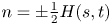 $n = \pm {\tfrac{1}{2}} H(s,t)$, the kinematic conditions are (Van De Fliert et al. Reference Van De Fliert, Howell and Ockenden1995; Ribe Reference Ribe2001)
 \begin{equation} \left(1\mp \frac{1}{2} \kappa H \right) \left( {v} \mp \frac{1}{2} \frac{\partial H}{\partial t} \right) ={\pm} \frac{1}{2}\frac{\partial H}{\partial s} \left( {u} \pm \frac{1}{2} H \frac{\partial \theta}{\partial t} \right), \end{equation}
and demanding that these surfaces are stress-free implies
 \begin{gather} \left(1\mp \frac{1}{2} \kappa H \right) \sigma_{sn} \mp \frac{1}{2} \frac{\partial H}{\partial s} \sigma_{ss} = 0, \end{gather}
 \begin{gather}\left(1\mp \frac{1}{2} \kappa H \right) \sigma_{nn} \mp \frac{1}{2} \frac{\partial H}{\partial s} \sigma_{sn} = 0. \end{gather}
We neglect surface tension primarily for simplicity; its inclusion would give rise to additional terms on the right of (2.11) and (2.12) involving the local curvature.
2.3. Constitutive model
We write the Oldroyd-B constitutive model (Bird & Wiest Reference Bird and Wiest1995) as
 \begin{equation} \boldsymbol{\sigma} ={-} p \boldsymbol{\delta} + \hat\eta_s \dot{\boldsymbol{\gamma}} + \boldsymbol{\tau}, \end{equation}
where  $p$ is the pressure,
 $\hat \eta _s$ is a viscosity,
 $\dot {\boldsymbol {\gamma }}$ is twice the rate of strain tensor and the viscoelastic stress
 $\boldsymbol {\tau }$ satisfies
 \begin{equation} \frac{1}{\hat E} \overset{\triangledown}{\boldsymbol{\tau}} + \frac{1}{\hat\eta}{\boldsymbol{\tau}} = \dot{\boldsymbol{\gamma}},\end{equation}
where  $\hat {E}$ is an elastic modulus,
 $\hat \eta$ is a viscosity and
 $\overset {\triangledown }{}$ denotes the upper convected derivative. If
 $\hat {\eta }_{s} =0$, (2.14) reduces to a Maxwell model; (2.14) limits to a viscous fluid if
 $\hat {E} \to \infty$, and an incompressible elastic material for
 $\hat {\eta } \to \infty$. The latter limit, coupled with a finite
 $\eta _s$, represents a Kelvin model. In common with other literature using this model, we refer to
 $\eta _s$ as the ‘solvent’ viscosity, although it does not necessarily need to represent such a physical effect;
 $\eta _s$ could also represent the effect of a ‘plasticiser’ added to make a polymeric material more malleable, or be simply treated as a regularisation parameter that precludes instantaneous (elastic) deformation. Similarly, we informally refer to
 $\eta$ as the ‘polymer’ viscosity, without necessarily implying that the microstructure responsible is a polymer.
2.4. Scaled equations
Given a characteristic thickness  $\mathcal {H}$ and length
 $\mathcal {L}$ of the ribbon, we introduce a small parameter
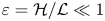 $\varepsilon =\mathcal {H}/\mathcal {L}\ll 1$. We then scale lengths, velocities, time and stress as
 \begin{align} s \sim \mathcal{L}, \quad n,H,\xi,\zeta \sim \mathcal{H} , \quad \kappa \sim \frac{1}{\mathcal{L}}, \quad {u},{v} \sim \mathcal{U}, \quad t \sim \frac{\mathcal{H}}{\mathcal{U}}, \quad \sigma_{ij},\tau_{ij},p \sim \mathcal{P}, \quad \dot{\gamma}_{ij} \sim \frac{\mathcal{U}}{\mathcal{L}}, \end{align}
and define the dimensionless groups and body force,
 \begin{equation} E = \frac{\varepsilon\hat{E}}{ \mathcal{P}}, \quad (\eta,\eta_s) = \frac{\mathcal{U}}{\mathcal{L} \mathcal{P}} (\hat{\eta},\hat{\eta}_s) , \quad (\,f_s,f_n) = \frac{\mathcal{L}}{\varepsilon \mathcal{P}} (\,\hat{f}_s,\hat{f}_n).\end{equation}
Here,  $\mathcal {U}$ and
 $\mathcal {P}$ denote typical scales for velocity and stress. It is possible to choose two of the parameters in (2.16a–c) to be unity by selecting the velocity and stress scales appropriately. For the moment, we retain all of them and proceed on the assumption that they are
 $O(1)$. With surface tension included, the additional terms on the right-hand side of (2.11) and (2.12) have a relative size of
 $\hat {\varGamma }/\mathcal {L}\mathcal {P}$, where
 $\hat {\varGamma }$ is the surface tension, so our neglect of these assumes that this group is small.
Avoiding any further change of notation for the dimensional and dimensionless coordinates and variables, the force balance equations become
 \begin{gather} \frac{\partial \sigma_{ss}}{\partial s} + \frac{1}{\varepsilon} (1-\varepsilon \kappa n) \frac{\partial \sigma_{sn}}{\partial n} - 2 \kappa \sigma_{sn} ={-} \varepsilon(1- \varepsilon\kappa n) f_s, \end{gather}
 \begin{gather}\frac{\partial \sigma_{sn}}{\partial s} + \frac{1}{\varepsilon} (1-\varepsilon\kappa n) \frac{\partial \sigma_{nn}}{\partial n} + \kappa (\sigma_{ss}-\sigma_{nn}) ={-} \varepsilon (1- \varepsilon \kappa n) f_n, \end{gather}
with surface conditions at  $n = \pm {\frac {1}{2}} H$,
 \begin{gather} \left(1\mp \frac{1}{2} \varepsilon\kappa H \right) \sigma_{sn} \mp \frac{1}{2} \varepsilon\frac{\partial H}{\partial s} \sigma_{ss} = 0, \end{gather}
 \begin{gather}\left(1\mp \frac{1}{2} \varepsilon\kappa H \right) \sigma_{nn} \mp \frac{1}{2} \varepsilon\frac{\partial H}{\partial s} \sigma_{sn} = 0. \end{gather}
The material derivative and continuity equation become
 \begin{gather} \frac{\textrm{D} }{\textrm{D} t} = \frac{\partial }{\partial t} + \varepsilon \left( {u} + \frac{\partial \theta}{\partial t} n \right) \frac{1}{1-\varepsilon\kappa n} \frac{\partial }{\partial s} + {v} \frac{\partial }{\partial n}, \end{gather}
 \begin{gather}\varepsilon\frac{\partial {u}}{\partial s} + (1- \varepsilon\kappa n) \frac{\partial {v}}{\partial n} - \varepsilon\kappa {v} = 0, \end{gather}
and the kinematic conditions on  $n = \pm {\frac {1}{2}} H$ are
 \begin{equation} \left(1\mp \frac{1}{2} \varepsilon\kappa H \right) \left( {v} \mp \frac{1}{2} \frac{\partial H}{\partial t} \right) ={\pm} \frac{1}{2}\varepsilon\frac{\partial H}{\partial s} \left( {u} \pm \frac{1}{2} H \frac{\partial \theta}{\partial t} \right). \end{equation}
In component form, in the curvilinear coordinate system, the constitutive equations are
 \begin{equation} \sigma_{ss} ={-}p + \tau_{ss} + {\eta}_s \dot{\gamma}_{ss}, \quad \sigma_{sn} = \tau_{sn} + {\eta}_s \dot{\gamma}_{sn}, \quad \sigma_{nn} ={-}p + \tau_{nn} + {\eta}_s \dot{\gamma}_{nn}, \end{equation}
where the viscoelastic stress is given by (see appendix A),
 \begin{gather} \frac{1}{E} \left[ \frac{\textrm{D} \tau_{ss}}{\textrm{D} t} - \frac{2\varepsilon}{1-\varepsilon\kappa n}\tau_{ss} \left( \frac{\partial {u}}{\partial s} - \kappa {v}\right) -2 \tau_{sn} \frac{\partial {u}}{\partial n} \right] + \frac{1}{\eta} \tau_{ss} = \dot{\gamma}_{ss}, \end{gather}
 \begin{gather}\frac{1}{E} \left[ \frac{\textrm{D} \tau_{sn}}{\textrm{D} t} - \frac{\varepsilon}{1-\varepsilon\kappa n}\tau_{ss} \left( \frac{\partial {v}}{\partial s} + \kappa {u} + \frac{1}{\varepsilon} \frac{\partial \theta}{\partial t} \right) - \tau_{nn} \frac{\partial {u}}{\partial n} \right] + \frac{1}{\eta} \tau_{sn} = \dot{\gamma}_{sn}, \end{gather}
 \begin{gather}\frac{1}{E} \left[ \frac{\textrm{D} \tau_{nn}}{\textrm{D} t} - \frac{2\varepsilon}{1-\varepsilon\kappa n}\tau_{sn} \left( \frac{\partial {v}}{\partial s} + \kappa {u} + \frac{1}{\varepsilon} \frac{\partial \theta}{\partial t} \right) - 2 \tau_{nn} \frac{\partial {v}}{\partial n} \right] + \frac{1}{\eta} \tau_{nn} = \dot{\gamma}_{nn}, \end{gather}
and
 \begin{gather} \dot{\gamma}_{ss} = \frac{2}{1-\varepsilon\kappa n} \left( \frac{\partial {u}}{\partial s} - \kappa {v} \right), \end{gather}
 \begin{gather} \dot{\gamma}_{sn} = \frac{1}{1-\varepsilon\kappa n} \left( \frac{\partial {v}}{\partial s} + \kappa {u} + \frac{1}{\varepsilon} \frac{\partial \theta}{\partial t} \right) + \frac{1}{\varepsilon} \frac{\partial {u}}{\partial n}, \quad \dot{\gamma}_{nn} = \frac{2}{\varepsilon} \frac{\partial {v}}{\partial n}. \end{gather}
2.5. Analysis of the scaled equations
From (2.17)–(2.20) we see that  $\sigma _{sn} = \tau _{sn} = O(\varepsilon )$ and
 $\sigma _{nn} = O(\varepsilon )$. Hence
 $p = -{\frac {1}{2}} \sigma _{ss} + {\frac {1}{2}} \tau _{ss} + {\frac {1}{2}} \tau _{nn} + O(\varepsilon )$, and therefore
 \begin{equation} \sigma_{ss} = \tau_{ss} - \tau_{nn} + 2 {\eta}_s \dot{\gamma}_{ss} + O(\varepsilon). \end{equation}
From (2.22) and (2.23) we have  ${v} = O(\varepsilon )$,
 $\partial H/\partial t = O(\varepsilon )$, and from (2.28a–c) we deduce
 \begin{equation} {u}(s,n,t) = \frac{\partial {\bar{\xi}}}{\partial t}(s,t) - \frac{\partial \theta}{\partial t}(s,t) n + O(\varepsilon), \end{equation}
where  ${\bar {\xi }}(s,t)$ is the average in-plane displacement across the sheet. Hence
 \begin{equation} \dot{\gamma}_{ss} = 2 \left( \frac{\partial^2 {\bar{\xi}}}{\partial s \partial t} - n \frac{\partial \kappa}{\partial t} \right) + O(\varepsilon), \end{equation}
so that, to leading order, the constitutive equations (2.25)–(2.27) become
 \begin{gather} \frac{1}{E} \frac{\partial \tau_{ss}}{\partial t} + \frac{1}{\eta} \tau_{ss} = 2 \left( \frac{\partial^2 {\bar{\xi}}}{\partial s \partial t} - n \frac{\partial \kappa}{\partial t} \right), \end{gather}
 \begin{gather}\frac{1}{E} \frac{\partial \tau_{nn}}{\partial t} + \frac{1}{\eta} \tau_{nn} ={-} 2\left(\frac{\partial^2 {\bar{\xi}}}{\partial s \partial t} - n \frac{\partial \kappa}{\partial t} \right). \end{gather}
Thus,  $\tau _{nn} = - \tau _{ss}$, and from (2.29) we find that the axial stress component
 $\sigma _{ss}$ satisfies
 \begin{equation} \left( \frac{1}{E} \frac{\partial }{\partial t} + \frac{1}{\eta}\right) \left[ \sigma_{ss} - 4 \eta_s \left( \frac{\partial^2 {\bar{\xi}}}{\partial s \partial t} - n \frac{\partial \kappa}{\partial t} \right) \right] = 4 \left( \frac{\partial^2 {\bar{\xi}}}{\partial s \partial t} - n \frac{\partial \kappa}{\partial t} \right). \end{equation}
We make use of this expression below in deriving width-integrated constitutive relations.
2.6. Width-integrated equations
Integrating the force balance equations (2.17) and (2.18) across the width of the sheet, and ignoring a term of order  $\varepsilon$, we find (Ribe Reference Ribe2002; Balmforth & Hewitt Reference Balmforth and Hewitt2013)
 \begin{gather} \frac{\partial N}{\partial s} - \kappa \frac{\partial M}{\partial s} ={-} H f_s, \end{gather}
 \begin{gather}\frac{\partial^2 M}{\partial s^2} + \kappa N ={-} H f_n, \end{gather}
where
 \begin{equation} N(s,t) = \frac{1}{\varepsilon} \int_{-(1/2) H}^{(1/2) H} \sigma_{ss} \, \textrm{d}n, \quad M(s,t) = \int_{-(1/2) H}^{(1/2) H} n \sigma_{ss} \, \textrm{d}n,\end{equation}
are the net axial stress and moment, respectively. Note that unless the curvature is  $O(\varepsilon )$ or the body force is
 $O(1/\varepsilon )$, (2.35) and (2.36) demand that
 $N$ is order one, rather than
 $O(1/\varepsilon )$ as it might otherwise appear to be from its definition.
These total force balance equations hold independently of the rheology of the material. The rheology enters when we now use (2.34) to relate  $M$ and
 $N$ to the deforming geometry. Integrating (2.34) and its moment across the width we obtain
 \begin{gather} \left( \frac{1}{E} \frac{\partial }{\partial t} + \frac{1}{\eta} \right) \left( \varepsilon N - 4 H \eta_s \frac{\partial^2 {\bar{\xi}}}{\partial s \partial t} \right) = 4 H \frac{\partial^2 {\bar{\xi}}}{\partial s\partial t}, \end{gather}
 \begin{gather}\left( \frac{1}{E} \frac{\partial }{\partial t} + \frac{1}{\eta} \right) \left( M + \frac{1}{3} H^3 \eta_s \frac{\partial \kappa}{\partial t} \right) ={-} \frac{1}{3}H^3 \frac{\partial \kappa}{\partial t}. \end{gather}
From the first of these we see that the requirement that  $N$ is
 $O(1)$ means that
 ${\bar {\xi }}(s,t)$ must also be
 $O(\varepsilon )$, so that the leading order strain rate (2.31) is all due to bending, a consequence of the assumed
 $O(1)$ curvature.
2.7. Model summary for  $\kappa =O(1)$

We now summarise the model derived above for order-one curvatures. The geometry is captured by the relations,
 \begin{equation} \frac{\partial \theta}{\partial s}=\kappa,\quad \frac{\partial X}{\partial s} = \cos\theta \quad \textrm{and} \quad \frac{\partial Y}{\partial s} = \sin\theta.\end{equation}
The axial and transverse force balance equations are (2.35) and (2.36), and we may set  $H = 1$ in view of the negligible changes to the thickness. The constitutive equation for
 $N$ in (2.38) serves primarily to demand that
 ${\bar {\xi }} = O(\varepsilon )$, and then reduces to a secondary diagnostic for higher-order corrections to
 ${\bar {\xi }}$ that we may discard. Nevertheless,
 $N$ still appears as a model variable in the force balance equations, highlighting how the tension is set by the requirement that the sheet remain essentially inextensible along the centreline. The model equations can then be summarised as
 \begin{gather} \frac{\partial N}{\partial s} - \kappa \frac{\partial M}{\partial s} ={-} f_s, \end{gather}
 \begin{gather}\frac{\partial^2 M}{\partial s^2} + \kappa N ={-} f_n, \end{gather}
 \begin{gather}\frac{1}{E} \frac{\partial M}{\partial t} + \frac{1}{\eta} M ={-} \frac{1}{3} \frac{\partial \kappa}{\partial t} - \frac{1}{3} \eta_s \left( \frac{1}{E} \frac{\partial^2 \kappa}{\partial t^2} + \frac{1}{\eta}\frac{\partial \kappa}{\partial t} \right). \end{gather}
The boundary conditions to be imposed on the system depend on the detailed configuration to be explored. Below, we give specific examples, and quote the relevant boundary conditions there.
2.8. Discussion
Note that for  $E\to \infty$, the model becomes viscous, with
 $M=-{\tfrac{1}{3}}(\eta +\eta _s)\frac {\partial \kappa }{\partial t}$, and recovers the constitutive law for a viscous ribbon without significant in-plane stretching (Buckmaster et al. Reference Buckmaster, Nachman and Ting1975; Ribe Reference Ribe2002; Ribe et al. Reference Ribe, Habibi and Bonn2012). This limit is also recovered, but with only the solvent viscosity, when
 $E=0$ and provided there is no elastic pre-stress locked into the ribbon (to create a permanent moment). If, on the other hand,
 $\eta _s\to 0$, we recover a Maxwell ribbon model, which demands that the elastic stress (or moment
 $M$) relax to zero in any final state. For
 $\eta \to \infty$, the law has a Kelvin form, which permits the beam to reach equilibrium states with finite elastic stress (bending moment). Note that we have written the constitutive relation (2.43) in differential form, but it is also possible to express it in integro-differential form, using the integrating factor
 $e^{Et/\eta }$ (cf. Gomez et al. Reference Gomez, Moulton and Vella2019).
Although we have derived the model for a viscoelastic fluid described by (2.14) using an asymptotic reduction of the governing equations, there are similarities with models for viscoelastic beams proposed previously in the solid mechanics literature (Kempner Reference Kempner1954; Minahen & Knauss Reference Minahen and Knauss1993). Those models are typically written down for relatively small deflections (whereas ours applies when the curvature is order one), and invariably ignore bending-induced tensions (i.e. fixing  $N$ and ignoring (2.35)). They do, however, allow for richer viscoelastic behaviour, in particular allowing for both instantaneous elastic response and relaxation towards a static equilibrium with finite stress. Such behaviour cannot emerge from the more fluid-like Oldroyd-B constitutive law (2.14), which only encompasses one of those (for
 $\eta _s \to 0$ or
 $\eta \to \infty$, respectively) and not both. Such a model is more consistent with the so-called standard linear solid model; a generalisation to include this additional behaviour requires the addition of a strain term of the form
 \begin{equation} -\frac{1}{3} E_1 \left( \frac{1}{E} \frac{\partial \kappa}{\partial t} + \frac{1}{\eta}\kappa \right), \end{equation}
to the right-hand side of (2.43), where  $E_1$ is a second elastic modulus corresponding to the long-term relaxed elastic state (cf. Kempner Reference Kempner1954). The replacement of the integrating factor
 $e^{Et/\eta }$ in the integro-differential version of (2.43) with a more general memory term also allows for a richer viscoelastic response with multiple time scales. However, at this stage, we lose the connection afforded by our asymptotic reduction to an underlying constitutive model formulated with the full governing equations.
3. Viscoelastic curling, drooping and buckling
3.1. Curling
We begin our exploration of the dynamics captured by the model in (2.40a–c)–(2.43), by considering a simple curling problem. A viscoelastic sheet, clamped at both ends, is deformed into an arc of a circle by rotating the angle of its ends. The ends are then released, allowing the sheet to uncurl in the absence of any body forces. If the ends are held such that no tension is induced, the sheet curls up uniformly:  $\kappa =\kappa (t)$ and
 $M=M(t)$. Thus, the entire ribbon evolves according to the constitutive law,
 \begin{equation} \frac{{\rm d} M}{{\rm d} t} + \frac{E}{\eta} M ={-} \frac{1}{3} \left[ E \left(1+\frac{\eta_s}{\eta}\right) \frac{{\rm d} \kappa}{{\rm d} t} + \eta_s \frac{{\rm d}^2 \kappa}{{\rm d} t^2} \right], \end{equation}
with  $\kappa (t)$ either fixed by the rotation of the end, or evolving freely such that
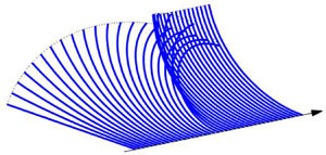
 $M(t)=0$. Figure 2(a) shows snapshots of a curled ribbon bent into a circle before being released, with
 $\kappa (t)=2{\rm \pi} t$ for
 $0<t<1$. Figure 2(b) plots the time series of
 $\kappa (t)$ and
 $M(t)$ both for this experiment, and for four others in which the end is either released earlier, or held fixed for a period before the release.
(a) Snapshots of a curling experiment in which a viscoelastic sheet is first curled up into a circle by controlling the angle of its ends, and then suddenly released (only half of the sheet is shown: the midpoint is fixed on the axis and the dotted line shows the locus of one of the controlled or free ends);  $E=\eta =1$ and
 $\eta _s=0.1$. In (b), we plot the time series of
 $\kappa (t)$ (the upper blue curves) and
 $M(t)$ (the lower green curves) for the experiment, along with four others in which the end is released earlier or held longer before release.

The controlled curl of the ribbon induces a bending moment that relaxes viscoelastically; the longer the curl develops or is maintained, the further the bending moment relaxes. As a consequence, when the ribbon is released, it uncurls for a period, but does not return to its original state and converges to a shape with finite curvature.
3.2. The viscoelastic cantilever
A more interesting example of the dynamics captured by the model in (2.40a–c)–(2.43) is the viscoelastic version of Galileo's cantilever. In this case, we impose a clamped end condition at  $s=0$ (so that
 $X(0,t)=Y(0,t)=\theta (0,t)=0$) and demand that the other end remain free (so that
 $M={\partial M}/{\partial s}=N=0$ at
 $s=1$). The cantilever then bends under a constant vertical gravity force with
 $f_s=-\sin \theta$ and
 $f_n=-\cos \theta$ (on selecting the stress scale
 ${\mathcal {P}}$ to set the amplitude of the gravitational force to unity).
A numerical solution to the model is shown in figure 3 for the relatively low value of the solvent viscosity  $\eta _s=0.01$ (appendix B provides details of the numerical schemes used for this computation, and for all our other model problems). In the limit
 $\eta \to \infty$, the model reduces to that for a Kelvin material, with the solvent viscosity controlling the time-dependent behaviour. For the current problem, the corresponding cantilever bends under gravity until the elastic stresses bring the beam to rest, as shown in figure 3(a). When
 $\eta$ is finite, however, the material creeps. For the cantilever, the consequence is that the beam does not reach a final state after the initial period of bending. Instead, the relaxation of the stress (and therefore the bending moment) implies that the beam cannot support itself against gravity over longer times, and continues to creep downwards until it becomes vertical (see figure 3b). Had the model incorporated changes in thickness, the long-time dynamics would then be dominated by a gradual thinning and extension. Capturing such changes requires a different scaling of the original equations that allows for larger axial stretching
 ${\bar {\xi }}$, or the inclusion of higher-order terms in the small parameter
 $\varepsilon$ (cf. Ribe Reference Ribe2001). The initial arrest of the fall and subsequent long-time creep is shown for a variety of values of
 $\eta$ in figure 3(c–f); over long times, evident are the increase of the curvature near the hinge, the relaxation of the bending moment and the emergence of a dominant tension as the beam becomes vertical and the tension balances its weight.
Snapshots of viscoelastic cantilevers for  $E=1$,
 $\eta _s=10^{-2}$ and (a)
 $\eta =\infty$ and (b)
 $\eta =10$. The dotted line shows the locus of the ends. On the right, we plot the maxima in (c)
 $|Y|$, (d)
 $|\kappa |$, (e)
 $|M|$ and (f)
 $|N|$. The points indicate the times of the snapshots in (a,b); the circles show the
 $\eta \to \infty$ solution. The dashed (red) lines show the expected, low-curvature, elastic solution
 $Y(X)=-X^2(X^2-4X+6)/8$ (which, from (2.40a–c)–(2.43), satisfies
 $s\approx X$,
 $M\approx -\frac 13 \kappa E$,
 $\kappa \approx Y''$,
 $M''\approx -1$,
 $N\approx 0$ and
 $Y(0)=Y'(0)=M(1)=M'(1)=0$).

3.3. Classical buckling
Without gravity or other body forces ( $f_n=f_s=0$), the model system (2.40a–c)–(2.43) admits an equilibrium solution corresponding to a straight viscoelastic beam subject to a compressive load, such that
 $\kappa =M=0$ and
 $N=N(t)$. Linear perturbations to this state satisfy
 \begin{equation} \theta=\frac{\partial Y}{\partial s}, \quad \kappa=\frac{\partial^2 Y}{\partial s^2}, \quad \frac{\partial^2 M}{\partial s^2}={-}\kappa N, \end{equation}
and
 \begin{equation} \left(1 + \frac{\eta}{E}\frac{\partial }{\partial t}\right) \left(N \frac{\partial^2 Y}{\partial s^2}\right) = \frac13 \eta \left( 1+ \frac{\eta_s}{\eta} + \frac{\eta_s}{E} \frac{\partial }{\partial t}\right) \frac{\partial^5 Y}{\partial t\partial s^4}, \end{equation}
where  $Y(s,t)$ is the small transverse displacement of the centreline (with
 $s\equiv x$ here).
For a constant load,  $N=N_0$, with clamped edge conditions,
 $Y=\theta =0$ at
 $s = \pm {\frac {1}{2}}$, we may take
 \begin{equation} Y \propto e^{\lambda t} [ 1-({-}1)^{j}\cos (2{\rm \pi} j s) ], \quad j=1,2,\ldots \end{equation}
to arrive at the growth rates,
 \begin{equation} \lambda = \frac{E}{2\eta_s} \left[\varPi_j-1-\frac{\eta_s}{\eta} \pm \sqrt{ \left(\varPi_j-1-\frac{\eta_s}{\eta}\right)^2 + 4 \frac{\eta_s}{\eta} \varPi_j}\right], \end{equation}
with
 \begin{equation} \varPi_j = \frac{3 |N_0|}{4{\rm \pi}^2j^2E}.\end{equation}
Figure 4 illustrates the two growth rates as functions of  $\varPi _j$ for a selection of values of the viscosity ratio
 $\eta _s/\eta$. One of these growth rates is always positive, proceeding monotonically from
 $\lambda \sim E\varPi _j/(\eta +\eta _s)$ for
 $\varPi _j\to 0$, to
 $\lambda \sim E\varPi _j/\eta _s$ for
 $\varPi _j\gg 1$. The elastic limit corresponds to taking
 $\eta \to \infty$, in which case
 $\lambda =\varPi _j-1$ or
 $\lambda =0$; the condition
 $\varPi _j=1$ is therefore the classical buckling threshold. Despite this, the viscoelastic beam remains unstable below
 $\varPi _j=1$, although the growth rate is much reduced for
 $\eta _s/\eta \ll 1$. This situation corresponds to what is referred to as ‘creep buckling’ in the solid mechanics literature (Kempner Reference Kempner1954; Hayman Reference Hayman1978; Minahen & Knauss Reference Minahen and Knauss1993), wherein creep permits deflections to grow unstably even below the elastic buckling threshold. In the viscous limit with
 $E\to \infty$, only the unstable mode with
 $\lambda \to E\varPi _j/(\eta +\eta _s)\equiv 3 |N_0| / [4 {\rm \pi}^2 j^2(\eta +\eta _s)]$ survives.
Growth rates of the linear buckling modes,  $\eta _s\lambda /E$, against the scaled load
 $\varPi _j$ in (3.6). Curves with
 $\eta _s/\eta = 10^{-3}$,
 $0.01$,
 $0.1$ and
 $0.3$ are shown; the dashed lines show the limit
 $\eta _s/\eta \to 0$.

Numerical solutions to the full problem (2.40a–c)–(2.43) for buckling under constant load are shown in figure 5(a,b). In these, we fix  $X = 0$ at the midpoint of the beam (
 $s = 0$) and assume symmetry about this, with
 $Y = \theta = 0$, and constant load
 $N = N_0$ at the end
 $s = {\frac {1}{2}}$. The solutions are initialised by adding the most unstable linear mode with a small amplitude to the basic (straight) state. For each panel, two solutions are shown: the load is below the elastic buckling threshold for one of these solutions, and above that threshold for the other. In panel (a) we show solutions for the Kelvin model with
 $\eta \to \infty$. In this limit there is no creep and the compressed beam below the buckling threshold remains stationary, with the initial shape frozen into the material. Above the threshold, the beam buckles and evolves over a time scale set by the solvent viscosity to the nonlinear state in which the lateral buckling is compensated by a reduction in the distance between the ends to preserve the overall length. For finite
 $\eta$ in panel (b), creep occurs, which allows the beam with lower
 $|N_0|$ to slowly deflect away from the initial shape (i.e. the phenomenon of creep buckling). The beam with higher
 $|N_0|$ again buckles rapidly towards the expected nonlinear elastic state, but the deflection then continues to grow under creep.
Snapshots of nonlinear buckling solutions,  $(X(s,t),Y(s,t))$, with
 $\eta _s=0.01$,
 $E=1$ and either
 $N_0=-11$ or
 $-15$, initiated with a small deflection from a straight beam. In (a) we show the solution for the Kelvin limit (
 $\eta \to \infty$), and in (b), we show the case with
 $\eta =10$, plotting half of the (symmetrical) beam in each case. The two solutions with
 $N_0=-11$ are offset for clarity, and the circles mark the ends of the beam. Dashed lines show the expected elastic solutions (satisfying (2.40a–c)–(2.42) with
 $M = - \frac 13 \kappa E$ and calculated numerically). In panel (c), we plot the maximum deflection
 $Y(0,t)$ of the solutions against time. The grey lines show the expected linear buckling behaviour, and points indicate the times of the snapshots in (a,b). The shapes of the two cases at the final time are shown in panel (d), with shading corresponding to local tension
 $N$.

3.4. Snap-through
For an elastic beam with clamped ends  $\theta (\pm {\frac {1}{2}},t)=0$ (satisfying (2.40a–c)–(2.42) with
 $M = - \frac 13 \kappa E$), there is an infinite number of buckled modes with thresholds given by
 $\varPi _j=1$, only the first of which (
 $j = 1$) is stable. When the end angles are controlled and varied away from zero, however, the finite-amplitude buckled solutions can become connected through a series of bifurcations (cf. Plaut & Virgin Reference Plaut and Virgin2009). In particular, the first mode
 $j=1$ can be connected to the third (
 $j=3$) by rotating the beam's ends counter to the direction of the buckle. The two solutions meet in a saddle-node bifurcation that destroys the stable elastic equilibrium; varying the end angle any further prompts a sudden ‘snap-through’ to the remaining stable equilibrium corresponding to a buckle with opposite sign.
Snap-through induced for a viscoelastic beam of Kelvin material ( $\eta \to \infty$) is shown in figure 6. In this example, a buckled state with horizontal ends is first generated by bringing the two ends together by a fixed distance of
 $0.1$. Imposing such end displacements in the full model (2.40a–c)–(2.43) is not completely straightforward and is achieved by a numerical regularisation scheme described in appendix B. For simplicity, we demand symmetry about
 $x=0$ (although elastic beams can also suffer symmetry-breaking bifurcations near snap-through; Plaut & Virgin Reference Plaut and Virgin2009). The ends are then rotated by periodically modulating
 $\theta ({\frac {1}{2}},t)$ between
 $1$ and
 $-1$ radians with a period of unity (for a symmetric solution
 $\theta (-{\frac {1}{2}},t)$ does the opposite). Figure 6(a) shows snapshots of the beam during half a cycle as
 $\theta ({\frac {1}{2}},t)$ is varied from
 $1$ to
 $-1$, which forces the solution to evolve through the saddle-node bifurcation, triggering snap-through; the solvent viscosity is relatively small (
 $\eta _s=0.01$), ensuring that the beam otherwise tracks the stable elastic equilibrium.
Buckled viscoelastic beams with periodically varying end angles  $\theta (\pm {\frac {1}{2}},t) = \cos (2{\rm \pi} t)$, for
 $\eta \to \infty$ and
 $E=1$, and with the horizontal distance between the ends being shortened by
 $0.1$. (a) Snapshots for equally spaced time intervals spanning half the cycle as
 $\theta ({\tfrac{1}{2}},t)$ varies from
 $1$ to
 $-1$ radians, for
 $\eta _s=0.01$. (b,d) Vertical displacement of the mid-point
 $Y(0,t)$ as a function of time over two cycles and (c,e) phase portraits on the
 $(\theta ({\frac {1}{2}},t),Y(0,t))-$plane, for
 $\eta _s = 10^{-3}$,
 $0.01$ and
 $0.05$ (b,c), and
 $\eta =0.15$,
 $0.2$ and
 $0.4$ (d,e). In (b,c), the dots correspond to the snapshots in panel (a). In (c,e), the stable elastic equilibrium solutions are shown as black lines, while the grey lines show unstable branches. The two red dashed lines in (a) show the elastic equilibria solution either side of the saddle node (calculated numerically from (2.40a–c)–(2.42) with
 $M = - \frac 13 \kappa E$), as indicated by the circles in (c).

The time series and phase portrait shown in figure 6(b,c) display the shadowing of the stable elastic equilibria and the sudden snap-through in more detail; the phase portrait, drawn on the 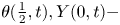 $\theta ({\frac {1}{2}},t),Y(0,t)-$plane, displays the elastic equilibria as black lines, with the superposed viscoelastic solution. The saddle-node bifurcations of the elastic states arise for end angles of
 $\theta \approx \pm 0.64$; in fact, the solution branches can be continued further, revealing more saddle-node bifurcations connecting to yet higher buckling modes (all of which are unstable; see the lighter lines in figure 6c,e).
Figure 6(b,c) also includes more viscoelastic solutions with different choices for  $\eta _s$. Increasing the solvent viscosity smooths the snap-through, at least up to
 $\eta _s=0.1$ or so, highlighting how this dissipative effect controls the dynamics here (cf. Gomez et al. Reference Gomez, Moulton and Vella2019). For higher solvent viscosities (
 $\eta _s$ above
 $0.15$), the dissipation slows the dynamics so much that snap-through is prevented entirely. Adding a polymer viscosity (finite
 $\eta$) complicates the dynamics yet further by introducing creep over longer time scales, but otherwise the model still predicts the occurrence and prevention of snap-through.
4. Small curvature and the viscoelastic catenary
The model outlined in § 2.7 and the examples in § 3 all relate to viscoelastica with order-one curvature (although we evolve the system from relatively straight states in the examples). When working with strictly small curvatures, however, some rescaling of the model is needed to account for the correspondingly smaller bending moments. Simultaneously, one must keep track of the  $O(\varepsilon )$ stretch associated with the axial displacement
 ${\bar {\xi }}$. In this section, we therefore rework the reduced model to suit this limit of the problem and apply the modified model to the fall of a viscoelastic catenary (cf. Roy et al. Reference Roy, Mahadevan and Thiffeault2006).
4.1. Small displacement equations
For small displacements from the horizontal under a weak vertical body force (with an appropriate choice of the stress scale), we rescale such that
 \begin{equation} (Y,\theta,\kappa,M,{\bar{\xi}})= \varepsilon ({\varUpsilon},\varTheta,{\mathcal{K}},{\mathcal{M}},{\mathcal{X}}), \quad f_n \approx f_y ={-}\varepsilon G, \quad f_s \approx f_x = 0, \end{equation}
where
 \begin{equation} \varTheta = \frac{\partial {\varUpsilon}}{\partial x}, \quad {\mathcal{K}} = \frac{\partial^2 {\varUpsilon}}{\partial x^2}. \end{equation}
We change from arc length  $s$ to straight-line distance
 $x$, with
 $-{\frac {1}{2}}<x<{\frac {1}{2}}$, noting that
 \begin{equation} \frac{\partial s}{\partial x} = 1 + \frac{1}{2} \varepsilon^2 \left(\frac{\partial {\varUpsilon}}{\partial x}\right)^2 + \cdots, \end{equation}
and define the geometrically induced stretch  $S$ as the relative change in the total arc length,
 \begin{equation} S(t) = \frac{1}{2} \int_{{-}1/2}^{1/2} \left(\frac{\partial {\varUpsilon}}{\partial x}\right)^2 \, \textrm{d} x. \end{equation}
The stretch is related to the total axial displacement  ${\mathcal {X}}$, by
 \begin{equation} {\mathcal{X}}({\tfrac{1}{2}} )-{\mathcal{X}}(-{\tfrac{1}{2}}) = S + \varDelta, \end{equation}
where  $\varDelta$ represents any relative horizontal displacement of the ends.
The rescaled equations of the model now take the leading-order form,
 \begin{gather} \frac{\partial N}{\partial x} = 0, \quad \frac{\partial^2 {\mathcal{M}}}{\partial x^2} + N \frac{\partial^2 {\varUpsilon}}{\partial x^2} = G, \end{gather}
 \begin{gather} \left( \frac{1}{E} \frac{\partial }{\partial t} + \frac{1}{\eta} \right) \left( N - 4 \eta_s \frac{\partial^2 {\mathcal{X}}}{\partial s \partial t} \right) = 4 \frac{\partial^2 {\mathcal{X}} }{\partial s\partial t}, \end{gather}
 \begin{gather}\left( \frac{1}{E} \frac{\partial }{\partial t} + \frac{1}{\eta} \right) \left( {\mathcal{M}} + \frac{1}{3} \eta_s \frac{\partial^3 {\varUpsilon}}{\partial x^2 \partial t} \right) ={-} \frac{1}{3}\frac{\partial^3 {\varUpsilon}}{\partial x^2 \partial t}. \end{gather}
Thence, eliminating  $M$ gives
 \begin{equation} \frac{1}{3} E \frac{\partial^5 {\varUpsilon}}{\partial x^4 \partial t} + \frac{1}{3} \eta_s \left(\frac{\partial}{\partial t} + \frac{E}{\eta} \right) \frac{\partial^5 {\varUpsilon}}{\partial x^4 \partial t} = \left(\frac{\partial}{\partial t} + \frac{E}{\eta} \right) \left( N \frac{\partial^2 {\varUpsilon}}{\partial x^2} - G \right), \end{equation}
and since  $N(t)$ is independent of space, the tension equation (4.7) can be integrated to give
 \begin{equation} \left( \frac{\partial}{\partial t} + \frac{E}{\eta} \right) N = 4 E \frac{\partial }{\partial t}(S+\varDelta) + 4 \eta_s \left( \frac{\partial}{\partial t} + \frac{E}{\eta} \right) \frac{\partial }{\partial t}(S+\varDelta). \end{equation}
Note that the tension evolution equation (4.10) permits a sudden change in strain  $\varDelta$ to generate a viscoelastically relaxing tension
 $N(t)$, which corresponds to the only effect of viscoelasticity in the model provided by Roy et al. (Reference Roy, Mahadevan and Thiffeault2006). By contrast, the current model captures the full viscoelastic relaxation of both the tension and moment.
4.2. Boundary and initial conditions
We impose symmetry around  $x = 0$, with the fluid clamped at
 $x = \pm {\frac {1}{2}}$, so we demand
 \begin{equation} \frac{\partial {\varUpsilon}}{\partial x} = \frac{\partial^3 {\varUpsilon}}{\partial x^3} = 0 \ \textrm{at} \ x = 0, \quad {\varUpsilon} = \frac{\partial {\varUpsilon}}{\partial x} = 0 \ \textrm{at } \ x = \frac{1}{2}, \end{equation}
When there is no additional strain on the ends, we set  $\varDelta =0$. The most straightforward way to initiate the fall of the viscoelastic catenary is to suddenly turn on the gravity force, starting from an initial state of rest with
 \begin{equation} {\varUpsilon} = 0, \quad \frac{\partial {\varUpsilon}}{\partial t} = 0, \quad N = 0 \ \textrm{at} \ t = 0. \end{equation}
The introduction of gravity ( $G = 1$ for
 $t>0$) then provides an impulsive forcing on the right-hand side of (4.9) that introduces a jump in the highest time derivative at
 $t=0$. For finite solvent viscosity, we therefore impose
 \begin{equation} \frac{1}{3} \eta_s \frac{\partial^5 {\varUpsilon}}{\partial x^4 \partial t} ={-} 1 \ \textrm{at} \ t=0, \end{equation}
which provides the initial velocity,
 \begin{equation} \frac{\partial {\varUpsilon}}{\partial t} ={-}\frac{1}{8\eta_s} \left( x^2 - \frac{1}{4} \right)^2 \ \textrm{at} \ t = 0. \end{equation}
On the other hand, if the solvent viscosity is zero, no initial condition for  $\partial {\varUpsilon }/\partial t$ is required. Instead, in view of our omission of inertia, the material instantaneously stretches to satisfy the elastic problem
 $\frac {1}{3}E {\varUpsilon }_{xxxx} - N {\varUpsilon }_{xx} = -G$, with
 $N = 4ES$. This has solution
 \begin{equation} {\varUpsilon} = {\varUpsilon}_{_E} \equiv \frac{3}{2Ek^2} \left( x^2-\frac14 + \frac{\cosh {\frac{1}{2}} k - \cosh kx}{k \sinh{\frac{1}{2}} k} \right), \quad N = \frac{Ek^2}{3}, \end{equation}
(for  $G=1$), where
 $k$ is given by
 \begin{equation} \int_0^{{1}/{2}} \left( \frac{\partial {\varUpsilon}_{_E}}{\partial x} \right)^2 {\rm d} x = \frac{k^2}{12}. \end{equation}
For  $N\ll 1$, we find
 \begin{equation} {\varUpsilon}_{_E} \to -\frac{1}{8E} \left( x^2 - \frac{1}{4} \right)^2 \quad \textrm{and} \quad N \to \frac{1}{1680E}.\end{equation}
If  $\eta \to \infty$, the catenary is purely elastic and the steady equilibrium solution is
 ${\varUpsilon }={\varUpsilon }_{_E}$.
4.3. Falling catenaries
For a viscous catenary (Teichman & Mahadevan (Reference Teichman and Mahadevan2003);  $E \to \infty$,
 $\eta _s=0$), the equations become
 \begin{equation} N = 4 \eta \frac{\partial S}{\partial t}, \quad \textrm{and} \quad \frac{1}{3} \eta \frac{\partial^5 {\varUpsilon}}{\partial x^4 \partial t} - N \frac{\partial^2 {\varUpsilon}}{\partial x^2} ={-} 1. \end{equation}
The early-time behaviour is dominated by viscous bending, with
 \begin{equation} {\varUpsilon} \sim \frac{1}{8\eta} \left( x^2 - \frac{1}{4} \right)^2 t, \quad S \sim \frac{t^2}{6720\eta^2}, \quad N \sim \frac{t}{840\eta }. \end{equation}
The large-time behaviour is dominated by stretching, with narrow bending boundary layers at the ends. Away from the latter,
 \begin{equation} {\varUpsilon} \sim \frac{9^{1/3}}{2\eta^{1/3}} \left( x^2 - \frac{1}{4} \right) t^{1/3}, \quad S \sim \frac{t^{2/3} }{24}\left(\frac{9}{\eta}\right)^{2/3},\quad N\sim \left(\frac{\eta}{9}\right)^{1/3} t^{{-}1/3}. \end{equation}
Numerical solutions for a falling viscoelastic catenary ((4.9) and (4.10)) are shown in figure 7. Panel (a) of the figure shows snapshots of the catenary with  $E=1$,
 $\eta =10$ and
 $\eta _s=0.01$. In this example, the catenary first falls by viscous bending with a viscosity set by
 $\eta _s$. Elastic stresses then come into play to arrest the fall close to the elastic equilibrium. At later times, creep sets in, re-activating the fall of the catenary, which then falls like a viscous material with viscosity
 $\eta$; this later fall is again primarily controlled by bending to begin with, as in (4.19a–c), but then slows when stretching takes over the force balance, as in (4.20a–c).
(a) Snapshots of a falling catenary for  $E=1$,
 $\eta _s=0.01$ and
 $\eta =10$. Below, we plot (b)
 ${\rm Max}(|{\varUpsilon }|)$ and (c)
 $N$ for solutions with the values of
 $\eta$ indicated (and the same values of
 $E$ and
 $\eta _s$). The dotted and dash-dotted lines show the early-time behaviour of viscous catenaries with viscosity
 $\eta _s$ or
 $\eta$ (respectively); i.e. (4.19a–c), with
 $\eta =\eta _s$ or
 $\eta =10$. The thinner dashed lines show the stretching dominated viscous evolution in (4.20a–c) with
 $\eta =\eta _s=0.01$. In all the panels, the thicker (red) dashed lines show the elastic equilibrium solution (4.17a,b).

Figure 7(b,c) shows solutions with different choices for  $\eta$, displaying the maximum downward displacement and tension. The duration of the quasi-steady elastic phase decreases as
 $\eta$ is made more comparable with
 $\eta _s$, and disappears entirely when
 $\eta _s>\eta$, at which point the solvent viscosity completely controls the evolution (see the solution for
 $\eta =10^{-3}$).
5. Adding a yield stress
5.1. Elasto-viscoplastic model
The model outlined in § 2 focusses on an Oldroyd-B fluid, and accounts for linear viscoelastic effects. This model can, however, be generalised by adding a yield stress  $\tau _Y$, below which the polymeric stresses are purely elastic, and above which they become viscoplastic. More specifically, we adopt the Bingham-Maxwell, visco-elasto-plastic constitutive law (cf. Saramito Reference Saramito2007; Prior et al. Reference Prior, Moussou, Chakrabarti, Jensen and Juel2016) in place of (2.14),
 \begin{equation} \frac{1}{\hat E} \overset{\triangledown}{\boldsymbol{\tau}} + \frac{1}{\hat\eta}{\max}\left(0,1 - \frac{\tau_Y}{\tau_I} \right)\boldsymbol{\tau} = \dot{\boldsymbol{\gamma}}, \end{equation}
where 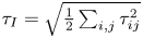 $\tau _I=\sqrt {{\frac {1}{2}}\sum _{i,j}\tau _{ij}^2}$ is the second invariant of
 $\boldsymbol {\tau }$. Other than adding the factor,
 ${\max}(0,1 - {\tau _Y}/{\tau _I})$, in front of the polymer viscosity terms and the introduction of a dimensionless yield-stress parameter,
 \begin{equation} B = \frac{\tau_Y}{{\mathcal{P}}}, \end{equation}
the reduction is much as in § 2. The main change is to (2.32), which becomes
 \begin{equation} \frac{1}{E} \frac{\partial \tau_{ss}}{\partial t} + \frac{\tau_{ss}}{\eta} {\max}\left(0,1-\frac{B}{|\tau_{ss}|}\right) = 2 \frac{\partial^2 {\bar{\xi}}}{\partial s \partial t} - 2n \frac{\partial \kappa}{\partial t}, \end{equation}
since  $\tau _{nn}=-\tau _{ss}$ and
 $\tau _I\approx |\tau _{ss}|$. This equation is similar to that used by Prior et al. (Reference Prior, Moussou, Chakrabarti, Jensen and Juel2016).
The width integrals of this equation, required to calculate  $N$ and
 $M$ as in (2.38) and (2.39), are no longer straightforward because of the nonlinear term on the left-hand side which gauges whether or not the fluid is yielded. In particular, one must now track the yield surfaces where
 $|\tau _{ss}|=B$. Some progress may be made by defining
 \begin{equation} \gamma_{p}(s,n,t) = \frac{\partial {\bar{\xi}}}{\partial s}-n \kappa - \frac{\tau_{ss}}{2E}, \end{equation}
which is the unrecoverable plastic contribution to the total strain (the first two terms on the right) that is not accommodated by the purely elastic deformation  $\tau _{ss}/2E$. The constitutive equation (5.3) can then be rewritten as the evolution equation,
 \begin{equation} \frac{\partial \gamma_{p}}{\partial t} = \frac{\varsigma E}{\eta} {\max}\left(0,\left|\frac{\partial {\bar{\xi}}}{\partial s}-n \kappa - \gamma_{p} \right|- \frac{B}{2E}\right), \end{equation}
where  $\varsigma =$ sgn
 $(\tau _{ss})=$ sgn
 $(\partial {\bar {\xi }}/\partial s-n \kappa - \gamma _{p})$. Given (2.29), we can then write the stress and moment resultants (for
 $H = 1$) as
 \begin{gather} \varepsilon N = 4 E \frac{\partial {\bar{\xi}}}{\partial s} + 4 \eta_{s} \frac{\partial^2 {\bar{\xi}}}{\partial s \partial t} - 4 E \int_{{-}1/2}^{1/2} \gamma_{p} {\,{\rm d}}n, \end{gather}
 \begin{gather}M ={-} \frac{1}{3} E \kappa -\frac{1}{3} \eta_s\frac{\partial \kappa}{\partial t} - 4 E \int_{{-}1/2}^{1/2}n \gamma_{p} {\,{\rm d}}n, \end{gather}
Note that if  $\gamma _{p}$ is an odd function of
 $n$ then (5.6) demands that
 ${\bar {\xi }} = O(\varepsilon )$. In this case, the evolution equation (5.5) demands that
 $\gamma _{p}$ remains odd in
 $n$. Hence, as in the viscoelastic theory of § 2,
 ${\bar {\xi }}$ must be small and can be neglected from the leading-order theory. (This conclusion is not valid if the tension N is
 $O(1/\varepsilon )$, as in the theory of Prior et al. Reference Prior, Moussou, Chakrabarti, Jensen and Juel2016).
To summarise, for order-one curvatures, the elasto-viscoplastic theory consists of the geometry and force balance equations (2.40a–c)–(2.42) as before, but with the constitutive law for the moment (2.43) replaced by (5.7), in which  $\gamma _{p}(s,n,t)$ evolves according to
 \begin{equation} \frac{\partial \gamma_{p}}{\partial t} = \frac{\varsigma E}{\eta} {\max}\left(0,|n \kappa + \gamma_{p} |- \frac{B}{2E}\right), \quad \varsigma={-}\textrm{sgn}(n \kappa + \gamma_{p}). \end{equation}
In general (5.8a,b) must be solved at each point in  $n$, as well as
 $s$, which makes the formulation less satisfying than a width-integrated theory. On the other hand, further progress is possible when the yielded region is always expanding and the ribbon is free of any plastic strains at the outset. In this situation,
 $\gamma _{p}=0$ over the unyielded regions, allowing for a useful width integral of (5.8a,b), as discussed in § 5.3 below.
Note that if  $B = 0$, the width integrals of (5.8a,b) give
 \begin{equation} \left( \frac{\partial }{\partial t} + \frac{E}{\eta} \right) \int_{{-}1/2}^{1/2} \gamma_{p} {\,{\rm d}}n = 0, \quad \left( \frac{\partial }{\partial t} + \frac{E}{\eta} \right) \int_{{-}1/2}^{1/2} n \gamma_{p} {\,{\rm d}}n ={-} \frac{E}{12\eta} \kappa, \end{equation}
and inserting these into (5.6) and (5.7) recovers the viscoelastic constitutive laws in (2.38) and (2.39). Conversely, if  $B \to \infty$, the material never yields, so
 $\gamma _{p} = 0$ and the constitutive laws (5.6) and (5.7) reduce to those of the Kelvin model. In the limit
 $E\to \infty$, the elastic deformation of the material becomes negligible and
 $\gamma _{p} \to - n \kappa$. It can then be deduced from (5.8a,b) that the sheet must either be unyielded across its whole width, in which case
 $\partial \kappa /\partial t = 0$, or it must yield throughout. Expanding (5.8a,b) for large
 $E$ now gives
 \begin{equation} \gamma_{p} \sim{-}n \kappa + \frac{1}{E} \left[ \eta n \frac{\partial \kappa}{\partial t} + \textrm{sgn}\left(n \frac{\partial \kappa}{\partial t}\right) \frac{B}{2} \right] + \cdots, \end{equation}
which, from (5.7), implies
 \begin{equation} M ={-}\frac{1}{3} (\eta_s+\eta) \frac{\partial \kappa}{\partial t} - \frac{1}{2} \textrm{sgn}\left( \frac{\partial \kappa}{\partial t} \right) B. \end{equation}
Note from the definition of  $\gamma _{p}$ in (5.4) that this also means the axial stress is given by
 \begin{equation} \tau_{ss} \sim{-}2 \eta n \frac{\partial \kappa}{\partial t} - \textrm{sgn}\left(n \frac{\partial \kappa}{\partial t}\right) B. \end{equation}
A stress jump therefore arises across the centreline of the sheet, and we recover the analysis of a viscoplastic ribbon presented by Balmforth & Hewitt (Reference Balmforth and Hewitt2013). For finite  $E$, the jump in stress is smoothed by elastic deformation across a small unyielded region surrounding the centreline.
5.2. Curling revisited
We now revisit the problem of § 3.1, in which a sheet is gradually curled up by imposing the angle of its ends, and then subsequently allowed to relax with no applied forces. Again, the dynamics are independent of arc length  $s$. There is an initial phase wherein the curvature
 $\kappa (t)$ is prescribed and the bending moment evolves accordingly, followed by a second phase in which the curvature evolves without any bending moment. The only equations to solve for this problem are those from the constitutive law, namely (5.7) and (5.8a,b). We consider, in particular, the curling problem in which the ribbon is initially curled up into a circle and then held for a period, so that
 $\kappa (t)=2{\rm \pi} t$ for
 $0\leq t\leq 1$,
 $\kappa (t)=2{\rm \pi}$ for
 $1\leq t\leq 2$, and
 $M(t)$ and
 $\gamma _{p}(n,t)$ are the unknowns. Subsequently, for
 $t>2$, we set
 $M = 0$, and solve for the unknowns
 $\kappa (t)$ and
 $\gamma _{p}(n,t)$.
Solutions are shown in figure 8 for various choices of the yield-stress parameter  $B$. For
 $B = 0$ the solution is similar to one shown earlier in figure 2. If
 $B>2{\rm \pi}$, the material never yields, and in that case the long-term behaviour is purely elastic: the sheet uncurls to its original flat state on a time scale set by the solvent viscosity. For intermediate values of
 $B$, the expanding yielded region occupies
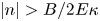 $|n| > B/2E\kappa$ as the curvature
 $\kappa$ increases past
 $B/E$ (the value at which the surfaces
 $n = \pm {\frac {1}{2}}$ yield), whilst the central region
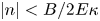 $|n| < B/2E\kappa$ remains unyielded. When the sheet is released and the curvature decreases, the yielded region shrinks again. At this stage, the yield surfaces are no longer related directly to the curvature, but depend on the extent to which the plastic strain has accommodated the excess stress. Eventually the stress falls below the yield stress everywhere, and the sheet then relaxes towards a new elastic equilibrium.
Curled elasto-viscoplastic ribbon solutions, showing (a) curvature and (b) bending moment with  $B = 0, 1, 3$ or
 $7$,
 $E = 1$,
 $\eta = \frac {1}{2}$ and
 $\eta _s = \frac {1}{3}$. Here,
 $\kappa = 2{\rm \pi} \, {{\rm min}}(t,1)$ is imposed for
 $0<t\le 2$, and
 $M = 0$ for
 $t>2$. The stars in (a) mark the prediction from (5.15). Panels (c) and (d) show respectively the plastic strain
 $\gamma _{p}(n,t)$, and the axial stress
 $\tau _{ss}(n,t)$ for the case
 $B = 1$, with the lines marking the position of the yield surfaces.

As is clear from (5.7), the final state has curvature  $\kappa _f$ given by
 \begin{equation} \kappa_f ={-}12 \int_{{-}1/2}^{1/2} n \gamma_{p} {\, {\rm d}}n. \end{equation}
Moreover, if the curled sheet is held at its maximum curvature  $\kappa _m$ for sufficient time that the stress fully relaxes over the yielded region, the plastic strain from (5.5) is given by
 \begin{equation} \gamma_{p} ={-}n \kappa_m {\max}\left(0,1-\frac{B}{2E|n| \kappa_m} \right). \end{equation}
In this case (provided  $\kappa _m > B/E$), the final state has curvature
 \begin{equation} \kappa_f = \kappa_m - \left(3-\frac{B^2}{E^2\kappa_m ^2} \right) \frac{B}{2E}, \end{equation}
which is included in figure 8.
5.3. Expanding yielded regions and the viscoplastic cantilever
When the fluid is free of any plastic strain at the outset, and deformations are such that the yielded region never shrinks, the unyielded sections remain free of plastic strain throughout, and the elastic stress there is given by  $\tau _{ss}=-2En\kappa$. The yield surfaces are therefore given by
 $|\tau _{ss}| = B$, or
 $n = \pm {\mathcal {Y}}(s,t)$ with
 \begin{equation} {\mathcal{Y}} = {\frac{1}{2}} {\min}\left(1,\frac{B}{E |\kappa|}\right).\end{equation}
The region  $|n|<{\mathcal {Y}}$ is unyielded with
 $\gamma _{p} = 0$, and so
 \begin{equation} \int_{{-}1/2}^{1/2} n \gamma_{p} {\, {\rm d}}n = 2 \int_{{\mathcal{Y}}}^{1/2} n \gamma_{p} {\, {\rm d}}n. \end{equation}
Integrating the first moment of (5.8a,b) over the width of the sheet now gives, after a little algebra,
 \begin{equation} \left( \frac{\partial }{\partial t} + \frac{E}{\eta} \right) \int_{{-}1/2}^{1/2} n \gamma_{p} \,\textrm{d}n = \frac{E}{4\eta} \left[ -\frac{1}{3} \kappa (1-8{\mathcal{Y}}^3) - \varsigma \frac{B}{2E}(1-4{\mathcal{Y}}^2)\right], \end{equation}
where  $\varsigma = -\textrm {sgn}(\kappa )$. Combining this with (5.7) then gives
 \begin{equation} \left(\frac{\partial }{\partial t} + \frac{E}{\eta}\right) \left(M + \frac{1}{3}E\kappa + \frac{1}{3} \eta_s \frac{\partial \kappa}{\partial t}\right) = \frac{E^2\kappa}{3\eta} (1-8{\mathcal{Y}}^3) + \frac{\varsigma BE}{2\eta} (1-4{\mathcal{Y}}^2). \end{equation}
This is the viscoplastic equivalent of (2.43), to which it reduces if  $B = 0$ (in which case
 ${\mathcal {Y}} = 0$).
To illustrate the behaviour of this model, we reconsider the drooping cantilever considered in § 3.2. To simplify the dynamics, we consider small deflections from the horizontal, so that the curvature  $\kappa$ is small and the body forces in (2.41) and (2.42) are given approximately by
 $(\,f_s,f_n)=(0,-1)$. With free end conditions, this implies that the tension is negligible and the bending moment is given by
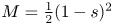 $M={\frac {1}{2}}(1-s)^2$. With
 $M(s)$ known and fixed, the (5.19) becomes an evolution equation for
 $\kappa (s,t)$ (with
 ${\mathcal {Y}}(s,t)$ given in terms of
 $\kappa$ by (5.16)). Having solved for
 $\kappa (s,t)$ we can then reconstruct the geometry.
Figure 9 shows sample solutions with differing yield stresses. For the example in panel (a), the yield stress is sufficiently strong that the gravitational stress does not breach the yield point at the clamped end; the ribbon deflects downwards elastically on the time scale controlled by the solvent viscosity, and then stops without any subsequent creep (cf. figure 3a). The final state is given by  $M=-E\kappa /3$, and since yielding occurs if
 $|\kappa | > B/E$, this solution is valid provided
 $B>3/2$ (
 $M={\frac {1}{2}}$ is maximum at the clamped end, where
 $\kappa = - 3/2E$).
Droop of an elasto-viscoplastic cantilever with  $E =1$,
 $\eta _s=0.1$ and
 $\eta =10$. Shown are snapshots of the centreline for (a)
 $B=2$, (b)
 $B=1.02$ and (c)
 $B=0.9$. The red dashed lines show the purely elastic equilibrium (cf. figure 3). In (b), the darker solid line is the final elasto-viscoplastic state. The insets in (b,c) show snapshots of the evolving yield surface
 ${\mathcal {Y}}(s,t)$, with darker solid lines showing (5.21). In (d), we plot
 $Y(1,t)$ for the three solutions; the dots indicate the times of the snapshots in (a–c).

The solution in figure 9(b) has a smaller  $B$ and as a result, the gravitational stress forces the ribbon to yield at the clamped end as the cantilever bends elastically. For the choice of viscosities used in the solution, bending slows as the ribbon approaches the elastic equilibrium. However, the yielded region at the clamped end introduces creep that permits the cantilever to continue its fall. Eventually, the creep bending subsides and the ribbon approaches an elasto-plastic equilibrium state for which (from (5.19))
 \begin{equation} M = \tfrac{1}{2} \varsigma B(1-4{\mathcal{Y}}^2)-\tfrac{8}{3}E\kappa{\mathcal{Y}}^3 \equiv \tfrac{1}{6} \varsigma B(3-4{\mathcal{Y}}^2), \end{equation}
provided  ${\mathcal {Y}}=-B/(2E\kappa )<{\frac {1}{2}}$. Hence
 \begin{equation} {\mathcal{Y}} = {\tfrac{1}{2}} \sqrt{3(1-2M/B)} = {\tfrac{1}{2}} \sqrt{3[1-(1-s)^2/B]}.\end{equation}
For the unyielded sections,  $\kappa =-3M/E$ and
 ${\mathcal {Y}}={\frac {1}{2}}$. Provided
 $B>1$, the yielded region therefore extends from the clamped end out to a position
 $s=s_*=1-\sqrt {2B/3}$, where
 $M=B/3$, with the ribbon remaining elastic beyond that point. Note that the ribbon does not yield anywhere (
 $s_*<0$) when
 $B>3/2$, consistent with the limit of the purely elastic solution mentioned above, so this solution is valid for the range
 $1<B<3/2$.
If  $B<1$, the solution in (5.21) ceases to exist near the clamped end where
 $1-(1-s)^2/B<0$, which corresponds to the complete failure of an elasto-plastic cantilever (Prager & Hodge Reference Prager and Hodge1951). This third situation is illustrated in figure 9(c). Now, because one cannot reach an elasto-plastic equilibrium near
 $s=0$, the cantilever continues to bend there, with the elastic core of the ribbon continuing to thin with time and the yield surfaces converging to the centreline,
 ${\mathcal {Y}}\to 0$. Again the choice of viscosities permits the ribbon to pause close to the elastic equilibrium, before unrestricted creep bending accelerates the fall of the free end (cf. figure 3a). Thus, if the yield stress is too small, the drooping of the cantilever cannot be halted, at least until much more significant drooping takes place (when the geometry change and induced tension are taken into account, the bending moment can be reduced and the yield stress may eventually halt the fall; cf. Balmforth & Hewitt Reference Balmforth and Hewitt2013).
6. Concluding remarks
In this article we have presented a reduced model for the curling, bending and buckling of a viscoelastica. We employed the standard Oldroyd-B model to describe the viscoelastic relaxation of the fluid, which leads to a model similar to beam theory for viscoelastic solids but allowing order-one curvatures. We used the model to explore the creation of permanent curls, the effect of creep on elastic buckling and snap-through, and the fall under gravity of cantilevers and catenaries.
Although we have used a rather simple constitutive law for viscoelasticity, the stretching rates of the sheet are found to be relatively small in these examples, when motions are primarily due to bending. Thus, many of the generalisations of Oldroyd-B to incorporate nonlinear viscoelastic effects related to polymer elongation (such as the FENE-type extensions) are unlikely to make a significant difference to our model reduction. Elasto-viscoplastic fluids, on the other hand, present a more significant variation on the model, in which plastic deformation only arises beyond a yield stress. As we have discussed in § 5, this generalisation of the model bridges to our earlier model for bending viscoplastic filaments (Balmforth & Hewitt Reference Balmforth and Hewitt2013) and the analysis of Prior et al. (Reference Prior, Moussou, Chakrabarti, Jensen and Juel2016) for the curling of ribbons.
Nevertheless, following on from the work of Ribe and co-workers (Ribe Reference Ribe2002; Ribe et al. Reference Ribe, Habibi and Bonn2012), one could continue the asymptotic analysis for slender sheets to higher order in order incorporate the more significant effects of stretching. The higher-order generalisation would then establish contact with existing theory for thinning viscoelastic threads (e.g. Chang, Demekhin & Kalaidin Reference Chang, Demekhin and Kalaidin1999; Clasen et al. Reference Clasen, Eggers, Fontelos, Li and McKinley2006).
Declaration of interests
The authors report no conflict of interest.
Appendix A. Dimensionless constitutive law
We write the dimensionless version of the constitutive law (2.14) in index form as
 \begin{equation} \frac{1}{E} \left( \frac{{\rm D}\tau_{ij}}{{\rm D}t} - \varepsilon \tau_{ik} \frac{\partial \hat{u}_j}{\partial x_k} - \varepsilon \frac{\partial \hat{u}_i}{\partial x_k} \tau_{kj} \right) + \frac{1}{\eta} \tau_{ij} = \dot{\gamma}_{ij} = \frac{\partial \hat{u}_i}{\partial x_j} + \frac{\partial \hat{u}_j}{\partial x_i}, \quad \end{equation}
where the material derivative is given by (2.21),  $\hat {\boldsymbol {u}} = \partial \boldsymbol {r}_c/\partial t + \boldsymbol {u}$ is the velocity and, in terms of the
 $(s,n)$ coordinate system, the stress and velocity gradient tensors are
 \begin{align} \boldsymbol{\tau} = \left( \begin{array}{cc} \tau_{ss} & \tau_{sn} \\ \tau_{sn} & \tau_{nn} \end{array} \right), \quad \boldsymbol{\nabla}\boldsymbol{\hat{u}} = \left( \begin{array}{cc} \left( \partial {u}/\partial s - \kappa {v}\right)/(1-\varepsilon\kappa n) & \varepsilon^{{-}1}\partial{u}/\partial n \\ \left( \partial{v}/\partial s + \kappa {u} + \varepsilon^{{-}1}\partial\theta/\partial t \right) /(1-\varepsilon\kappa n) & \varepsilon^{{-}1}\partial{v}/\partial n \end{array} \right). \end{align}
The three distinct components of this expression are as given in (2.25)–(2.28a–c).
Appendix B. Numerical methods
To solve the model in (2.40a–c)–(2.43) we discretise  $\kappa (s,t)$,
 $M(s,t)$ and
 $N(s,t)$ uniformly in
 $s$, and approximate spatial derivatives by finite differences. This results in a system of algebraic equations (2.41) and (2.42) for
 $M$ and
 $N$, coupled to a system of second-order ordinary differential equations (ODEs) (2.43) for
 $\kappa$. The latter is solved using a stiff ODE solver. Once the solution for
 $\kappa (s,t)$ is found the geometry is reconstructed from (2.40a–c) by quadrature, taking boundary conditions
 $\theta = X = 0$ at
 $s = 0$ and
 $Y = 0$ at one or other of the ends.
Three further boundary conditions are required, and given that the remaining spatial derivatives appear in (2.41) and (2.42), it is most straightforward if these are imposed on the stress resultants  $N$ and
 $M$. For the cantilever problem in § 3.2, this is indeed the case, with
 $N = M = \partial M/\partial s = 0$ at the free end. For the buckling problem in § 3.3 we assume symmetry and solve for only half of the domain
 $0<s<{\frac {1}{2}}$, allowing us to make use of the symmetry condition
 $\partial M/\partial s(0,t) = 0$. We also have an imposed load
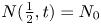 $N({\frac {1}{2}},t) = N_0$. To impose the final, clamped end condition,
 $\theta ({\frac {1}{2}},t) = 0$, we note that an integral of (2.43) implies the constraint,
 \begin{equation} \int_{0}^{1/2} M \,\textrm{d}s = 0,\end{equation}
(since  $\kappa = \partial \theta /\partial s$). This constraint completes the algebraic system that arises from the discretisation of (2.41) and (2.42), and which is solved at each instant of the time-stepping procedure.
The boundary conditions for the snap-through problem in § 3.4 are less straightforward to implement since they are all conditions on the end displacements or angles. This is not an issue for standard elastica or viscida problems, for which the moments are directly related to the displacements, but presents a difficulty in the current framework in view of the more complicated relation (2.43). The procedure we have adopted is to introduce a degree of slackness that allows us to impose conditions directly on the stresses. We again solve for only half of the domain  $0<s<{\frac {1}{2}}$, and apply the symmetry condition
 $\partial M/\partial s(0,t) = 0$. Then, for a desired end displacement
 $X({\frac {1}{2}},t) = {\frac {1}{2}}(1-\varDelta (t))$ and angle
 $\theta ({\frac {1}{2}},t) = \varTheta (t)$ we impose
 \begin{equation} N({\tfrac{1}{2}},t) = \frac{{\frac{1}{2}} (1-\varDelta(t))-X({\frac{1}{2}},t) }{\varepsilon_N}, \quad M({\tfrac{1}{2}},t) = \frac{\theta({\frac{1}{2}},t) - \varTheta(t) }{\varepsilon_M},\end{equation}
where  $\varepsilon _N$ and
 $\varepsilon _M$ are small parameters that control how tightly the conditions are satisfied. The conditions in (B 2) can be interpreted physically as representing the stiffness of the clamping device and as such may be a truer representation of some experimental arrangements than a hard constraint on the displacement and angle. For the simulations shown here we take
 $\varepsilon _N = 10^{-5}$ and
 $\varepsilon _M = 10^{-4}$.
For the catenary problem in § 4.3 we employ a similar procedure and discretise (4.9) uniformly in space, resulting in a system of second-order ODEs for  ${\varUpsilon }(s,t)$ that is coupled to the ODE (4.10) for
 $N(t)$. Boundary conditions on
 ${\varUpsilon }$ and its spatial derivatives are incorporated as part of the spatial discretisation, and the integral in (4.4) is calculated by quadrature using a finite difference approximation of
 $\partial {\varUpsilon }/\partial x$.
For the elasto-viscoplastic curling problem in § 5.2 we discretise  $\gamma _{p}(n,t)$ in
 $n$ and solve the resulting ODEs (5.8a,b) in time, coupled to (5.7), which is an ODE for either
 $M(t)$ or
 $\kappa (t)$. For the elasto-viscoplastic cantilever in § 5.3 we consider only small displacements so that the moment
 $M(s)$ is fixed. Then (5.19) for
 $\kappa (s,t)$ is discretised in
 $s$ and solved as a set of (decoupled) ODEs in time, from which the geometry is reconstructed by integrating
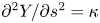 $\partial ^2 Y/\partial s^2 = \kappa$ subject to
 $Y(0,t) = \partial Y/\partial s(0,t) = 0$.



