Microwave nondestructive testing

The physical principle of microwave NDT relies upon disparities in the electrical properties of diverse media being tested. Notably, in noninvasive glucose detection utilizing microwave technology, the disparities in the conductivity σ and dielectric constant ε of the various tissues within the human body are substantial [Reference Turgul and Kale20]. Hence, it is feasible to ascertain the state of human health by transmitting and receiving signals via an antenna positioned on the skin’s surface. The changes in the dielectric features of human blood are mainly related to changes in blood glucose levels, with other substances in the blood, such as calcium and iron, having minimal or no effect on the variations in the dielectric characteristics of blood [Reference Sasaki, Wake and Watanabe21]. The Cole-Cole model provides a very effective and accurate measure of the changes in the dielectric properties of biological tissues over a wide range of frequencies. The dielectric constants of blood at different blood glucose concentrations are consistent with the first-order Cole-Cole model:

(1)\begin{equation}\% (\omega ) = {\varepsilon '_c}{\text{ }}(\omega ) - {\text{ }}j{\varepsilon '_c}{\text{ }}(\omega ) = {\text{ }}\varepsilon ,\frac{{{\text{ }}\Delta \varepsilon {\text{ }}}}{{1 + {\text{ }}(j\omega \tau )(1 - \alpha )}},\frac{{\sigma i}}{{j\omega \varepsilon }}\end{equation}

where ω is the angular frequency, ${\varepsilon '_c}{\text{ }}(\omega )$ is the frequency-dependent dielectric constant, ${\varepsilon '_c}{\text{ }}(\omega )$ is the frequency-dependent dielectric loss, ε _∞ is the frequency constant, Δε is the magnitude of the dispersion, τ is the relaxation time constant, α is a dispersion adjustment parameter that varies very little across body tissues, so its value is fixed at the mean value of 0.1. The calculated Cole-Cole parameters are fitted following the following second-order polynomials (2)–(5) [Reference Karacolak, Moreland and Topsakal22].

(2)\begin{equation}{\varepsilon _\infty }(x) = {a_n}{x^2} + {\text{ }}{b_n}x + {c_n}\end{equation}

(3)\begin{equation}\Delta {\varepsilon _n}(x) = {a_n}{x^2} + {\text{ }}{b_n}x + {c_n}\end{equation}

(4)\begin{equation}\tau (x) = {a_n}{x^2} + {\text{ }}{b_n}x + {c_n}\end{equation}

(5)\begin{equation}\sigma (x) = {a_n}{x^2} + {\text{ }}{b_n}x + {c_n}\end{equation}

In the above formula, x is the blood glucose concentration and its unit is mg/dL.

The values of the coefficients a_n, b_n and c_n are given in Table 1.

Table 1.

Coefficients of the cole-cole parameters

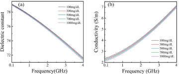
Using the above formula and combined with the parameters shown in Table 1, the fitting results of the dielectric characteristics with different glucose concentrations that change with the frequency are obtained, as shown in Fig. 1. The relationship between the dielectric constant and the conductivity of glucose solution at different glucose concentrations follows the frequency, where the frequency range is 0.1–4 GHz. The dielectric constant of glucose solution decreases with increasing frequency and increasing glucose concentration, and the conductivity increases with increasing frequency and decreasing glucose concentration. When glucose solutions with different glucose concentrations are tested using microwaves, the signal received will be altered due to the influence of the dielectric constant. By gauging and processing the changes in microwave signal parameters, the correlation between the glucose concentration and signal attenuation can be determined. Consequently, the objective of measuring glucose concentration can be realized.

To investigate the dielectric properties of different concentrations of glucose solutions, a variety of concentrations of glucose solutions were configured in the range of 100 mg/dL–1000 mg/dL with a concentration interval of 200 mg/dL. Experiments on the dielectric properties of glucose solutions using an open-ended coaxial probe and a vector network analyzer. Measurements were made with the measurement frequency angle set to 0.1 GHz-4 GHz.

The results of the dielectric properties of the glucose solution are shown in Fig. 2. Figure 2(a) shows the dielectric constants for different concentrations of glucose solutions and Fig. 2(b) shows the results of conductivity. It can be seen from Fig. 2 that in the frequency range of 0.1–4 GHz, the dielectric constant of the glucose solution gradually decreases with increasing frequency, while the conductivity then gradually becomes larger; at the same frequency, the dielectric constant of the glucose solution decreases with increasing concentration, and the conductivity also decreases with increasing concentration.

Figure 2.

Dielectric properties of glucose solutions: (a) dielectric constant, (b) conductivity.

Comparing the numerical calculation results of the dielectric properties of glucose solution with different glucose concentrations in Fig. 1, the measurements and numerical calculation results are highly similar in the same frequency band from 0.1 GHz to 4 GHz, both numerically and in terms of the variation pattern. The results demonstrate the change in glucose concentration causes its dielectric constant and conductivity changes.

Extreme learning machine

Efficient processing and analysis of microwave NDT glucose concentration signals necessitate efficient machine-learning algorithms. In this regard, the ELM algorithm has shown great adaptability in processing microwave glucose signals. The ELM algorithm can effectively extract and represent the relevant features of the microwave glucose signal to achieve accurate prediction of glucose concentrations, which is inherently complex and high-dimensional due to the presence of noise and interference.

ELM is a single-hidden layer feedforward neural network algorithm [Reference Yang, Zhang, Wang, Li and He23] based on the generalized Moore–Penrose proposed by Huang. It mainly solves the problems of slow SLFN learning speed, long iteration time, learning step size, learning rate, and other parameters that need to be set in advance. Compared to traditional neural network learning algorithms, the ELM algorithm is a much faster and more efficient way of processing, requiring only the appropriate number of nodes in the hidden layer, randomly generating all the parameters required for the hidden layer, and using least squares to determine the weights of the output layer [Reference Zheng, Hong, Wang and Chen24]. The whole learning process has only one step, without updating the hidden layer parameters.

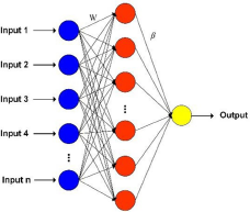
Figure 3 shows the structure of an ELM. For the supervised learning, containing the N data samples ((x, y) ∈ R^r × R^s), the training process consists of two stages. In the first stage, the input weight matrix W and the input threshold B are randomly generated according to the number of nodes in the hidden layer. In the second stage, the output matrix β is obtained by solving the least squares based on the data labels. The model is as follows.

(6)\begin{equation}y = \beta g\left( {Wx + b} \right)\end{equation}

Figure 3.

ELM network structure.

where W is the weight vector from the input layer to the hidden layer; b is the bias vector; g(·) is the activation function; and β is the output weight from the hidden layer to the output layer. The training process of the ELM network is the least squares solution β of the solution formula (7), and the output weight matrix β can be solved by the Moore-Penrose generalized inverse formula, as shown in Equation (8).

(7)\begin{equation}H\beta = Y\end{equation}

(8)\begin{equation}\beta = H^{\dagger }Y\end{equation}

(9)\begin{equation}H^{\dagger } = {\left( {{H^T}H} \right)^{ - 1}}{H^T}\end{equation}

Figure 4.

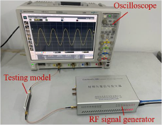
Measurement setup for glucose concentration detection.

Figure 5.

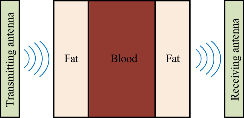
Schematic of the experimental detection process.

where H refers to the output matrix of the hidden layer, Y is the matrix of true values of the sample target outputs. H ^† is the generalized inverse of H, as shown in Equation (9). Due to the rapid learning ability, ELM is favored by researchers. In practice, ELM and its improved algorithms are widely used in fault detection, time series prediction, attitude recognition, chemical analysis, medical diagnosis, and intelligent power supply. The ELM algorithm has several advantages in addition to its adaptability in the processing of microwave glucose signals. First, the ELM algorithm can adjust its model parameters to improve regression accuracy according to different application requirements. Second, the ELM algorithm is fast to train and computationally inexpensive enabling it to handle large amounts of data and improve data processing efficiency. Third, the ELM algorithm can be combined with other data processing techniques such as principal component analysis and wavelet transform to further improve the accuracy and reliability of glucose level prediction.

Figure 6.

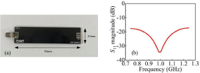
(a) The antenna used in the system. (b) S₁₁ parameter diagram of the antenna.

Therefore, the ELM algorithm stands as an efficient method for processing and analyzing microwave signals in noninvasive glucose detection, holding significant potential in the field. It provides valuable research references for the processing of microwave noninvasive detection of glucose concentration signals.

Experiment and result

A microwave-based noninvasive glucose testing system is constructed experimentally using microwave pulse signals at a single frequency point at 1 GHz for noninvasive glucose concentration detection. The whole experimental test system is shown in Fig. 4. The test system uses the RF Vector Signal Generator ENF860XC as the transmitting source of the microwave detection signal. The Oscilloscope Agilent Technologies DSO9404A is used to display and record the received microwave time-domain signals. Two antennas are used for the detection of the model under test. One of the antennas (transmitting antenna) is connected to a signal generator to transmit the signal. Meanwhile, another antenna (receiving antenna) is connected to an oscilloscope to collect the signal. The specific detection process is shown in Fig. 5. The microwave signal will be transmitted to the fat-blood-fat testing model for NDT through the transmitting antenna on one side of the testing model, and the detected microwave signal will be received by the receiving antenna on the other side.

The antenna used for the experimental tests is a planar ultra-wideband monopole antenna as shown in Fig. 6(a). The size of the antenna is 80 mm × 20 mm, and the bandwidth is 0.3–3.0 GHz. The S₁₁ parameter of the antenna is shown in Fig. 6(b).

Two antennas are fixed on each side of the glucose model to be measured, for transmitting and receiving microwave time-domain signals, respectively. In this experiment of simulated measurements, a sinusoidal microwave signal is chosen to detect glucose concentrations for the following reasons: First, compared to ultra-wideband microwave signals, single-frequency microwave signals are easier to obtain and perform more consistently in experimental tests. In addition, single-frequency microwave signals are simpler and easier to use and test in practice, making them more suitable for practical applications. If the single-frequency microwave signal performs well in experimental tests, then it means that the signal can also be a reliable way to select a microwave NDT signal. Therefore, to obtain more accurate test results and to combine the resonant performance of the antenna used, a continuous sinusoidal microwave signal with a frequency of 1 GHz and a power of 10 dBm is used for the noninvasive glucose detection.

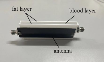
The glucose detection model used in the experiment is shown in Fig. 7, the whole model to be tested consists of the middle blood layer and the fat layer on both sides of the blood layer, the size of the model to be tested is 80 mm × 30 mm × 6 mm, among which the thickness of the blood layer is 3 mm and the thickness of the fat layer is 1.5 mm. In the actual test, polyformaldehyde resin (POM) material is used instead of fat. The dielectric constant of POM is about 3.7, which is similar to fat. The dielectric constant of POM is more stable, less susceptible to changes in humidity and temperature of the environment, and less affected by changes in frequency, so it is used instead of fat in this experiment. As blood is more difficult to obtain and store, the glucose solution is injected into the blood layer.

Figure 7.

Glucose testing model.

Figure 8.

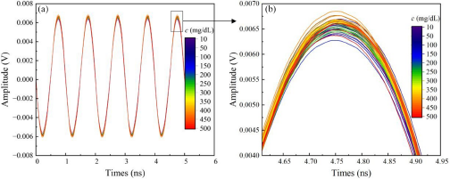
(a) The time domain of these detected signals with glucose solution concentrations ranged from 10 to 500 mg/dl with a step of 10 mg/dl, (b) the amplified portion of the time-domain received signal.

To obtain the test results at different glucose concentrations, different concentrations of glucose solution are configured. The actual normal glucose level in humans is 70–140 mg/dL, while in diabetic patients it can vary from 30 to 500 mg/dL [Reference Pathirage, Roopasinghe, Sooriyaarachchi, Weththasinghe and Nanayakkara13]. Given the actual situation and the needs of the study, the glucose solution is set in the range of 10–500 mg/dL. This range can cover all possible values that can be measured in clinical treatment. The concentration range of the glucose solutions configured in the experiment is 10–500 mg/dL with a concentration interval of 10 mg/dL, for a total of 50 groups, in which four-fifth is the training set and one-fifth is the test set. The time-domain detection signal recorded using an oscilloscope is shown in Fig. 8. In this case, Fig. 8(b) shows the time-domain signal locally amplified at the crest of a cycle. It can be seen from the figure that although there are some differences in the time domain between the signals measured for different concentrations of glucose solutions, these differences are not directly related to their corresponding concentrations and therefore the differences in concentration cannot be directly distinguished in the time domain and further processing and analysis of the data is required.

To identify the glucose concentration information carried in the microwave signals, a total of six parameters are extracted as input features, including maximum value x_max, minimum value x_min, peak-to-peak value p, root mean square (RMS) r, variance v, and standard deviation s of the time-domain waveform in each cycle. The specific equations describing these six time-domain characteristic parameters are shown in Table 2.

Table 2.

Expressions for time-domain features

The maximum value of a time-domain signal represents the highest value, and the minimum value represents the lowest value within a specified period. The difference between the maximum and minimum values of a signal is the peak-to-peak value and characterizes the amplitude range of the time-domain signal. The RMS is the square root of the average of all squared signal values over a given period. The RMS indicates the energy of the signal and measures the power of the signal. The variance of a signal represents the average of the squared differences between the signal value and its mean value over a given period. The standard deviation, also known as the mean square deviation, represents the degree of dispersion of the data and provides a visual representation of the typical deviation of a signal from its mean value.

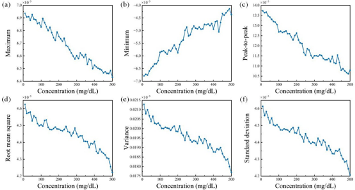
The features of the data set are extracted. The specific extraction results of the data set for each time-domain feature are shown in Fig. 9. There is a general trend of the time-domain features of the different concentrations of glucose solutions decreasing or increasing with concentration. Based on the six different time-domain features extracted, a dataset composed of 50 solution concentrations is formed with 6 × 50 dimensions.

Figure 9.

The features of the dataset based on time-domain signals: (a) maximum, (b) minimum, (c) peak-to-peak, (d) root mean square, (e) variance, (f) standard deviation.

To improve the accuracy and reliability of data processing, this paper normalizes the sample data to be processed. Data normalization refers to the scaling of different data features to a similar range to eliminate the effects of dimensionality. In practice, statistical analysis and modeling may result in certain features possibly being given higher weights or more attention due to the different units and scales of the features, and end up with biased or erroneous results. In order to avoid these effects, data from all glucose solution test samples are normalized using Equation (10):

(10)\begin{equation}{x^*} = \frac{{x - {x_{min}}}}{{{x_{max}} - {x_{min}}}}\end{equation}

where x represents the original glucose solution test sample data, x* represents the normalized sample data, and x _min and x _max represent the minimum and maximum values of the glucose solution test sample data, respectively. The normalized glucose solution test sample data eliminate the proportional differences between data features, making the data more comparable and improving the stability and accuracy of data processing.

The extracted feature data are processed for training using the ELM algorithm. After processing, the received signals of 50 sets of glucose solutions with concentrations ranging from 10 to 500 mg/dL and interval concentrations of 10 mg/dL, 6 × 50 data sets can be obtained. To verify the accuracy and reliability of the final estimates, we test the model repeatedly using fivefold cross-validation. The specific steps are as follows: First, we divide all the sample data into five parts equally and then take four of them as a training set and one aside as a test set. Next, we repeat this training process five times, each time selecting a different test set. This approach ensures that the performance evaluation of the model is not affected by specific data divisions.

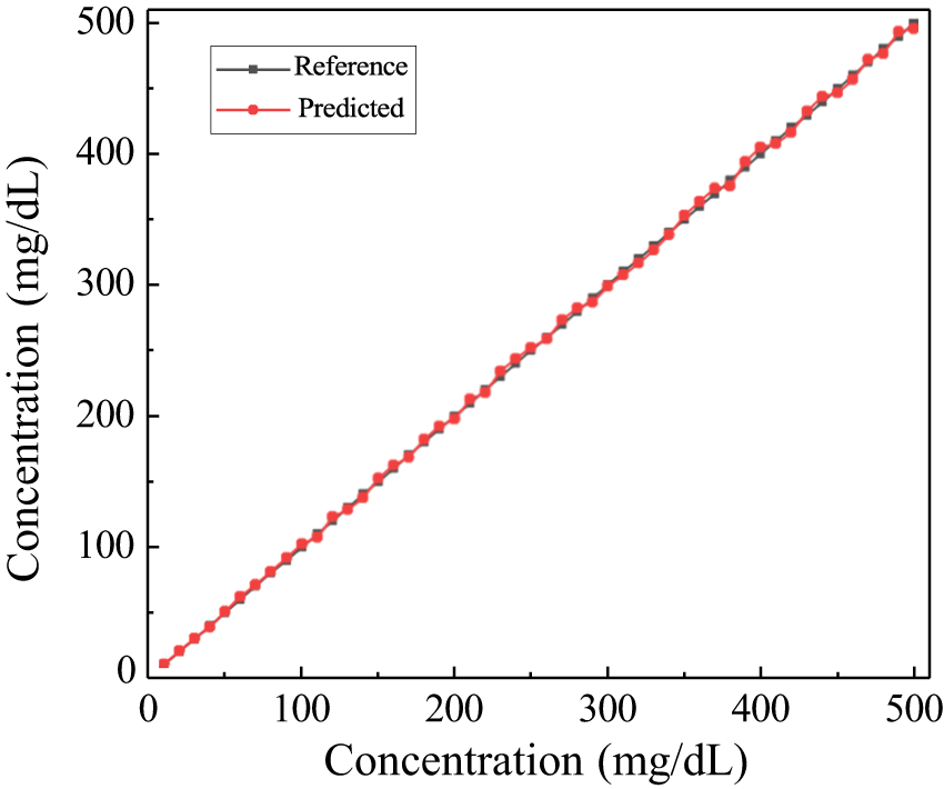
Figure 10 shows the results of the ELM-based glucose predictions by repeating the test five times. As can be seen from the figure, each glucose prediction (red dots) is very close to the corresponding label (black dots). The results show that accurate prediction of glucose concentration can be achieved using the ELM algorithm proposed in this paper.

Figure 10.

Comparison of prediction results obtained by ELM algorithm.

To evaluate the detection performance and accuracy of this algorithm more accurately and specifically, this paper uses two algorithm evaluation metrics, relative error (RE), and root mean square Error (RMSE), to evaluate the prediction results.

RE is the ratio of the absolute difference between the estimated result, minus the true value, and the true value. The expression for RE is shown in Equation (11). The RE assessment index can be used to evaluate the accuracy of the method, and when the RE is smaller, it means that the method is more accurate in predicting.

(11)\begin{equation}{\text{RE}} = \frac{{\left| {{c_p} - c} \right|}}{c} \times 100\% \end{equation}

where c_p refers to the concentration predicted by the algorithm and c refers to the true concentration of the solution.

RMSE is the sum of the squares of the differences between the predicted and true values divided by the number of samples and then the root number. The smaller the RMSE, the smaller the difference between the predicted and true values, and the higher the prediction accuracy of the model. Unlike the RE assessment metric, the RMSE is not affected by the size of the sample values and the specific expression for the RMSE is as follows:

(12)\begin{equation}{\text{RMSE}} = \sqrt {\frac{1}{n}\sum\limits_{i = 1}^n {{{\left( {{c_p} - c} \right)}^2}} } \end{equation}

Similarly, c_p in Equation (12) refers to the concentration predicted by the algorithm, c refers to the actual concentration of the solution, and n is the number of samples.

Table 3 shows the concentration results and REs predicted by the ELM algorithm for one of the fivefold cross-validations.

Table 3.

Predicted concentration and relative error

Table 4 shows all the error results obtained from the fivefold cross-validation. The average RE in the prediction of glucose solution concentration using the ELM method proposed in this paper is 1.45% with an RMSE of 2.56 mg/dL, and the maximum RE is 3.22%.

Table 4.

Results of the fivefold cross-validation

A comparison with other previous work is shown in Table 5. Huang and Omkar [Reference Huang, Yoshida, Inda, Xavier, Mu, Meng and Yu25] used the S11 and Z11 parameters to estimate the concentration of a glucose solution and obtained a maximum relative error (MMRE) of 12.8% based on a linear fitting method. In reference [Reference Hu, Nagae and Hirose26], the CVNN method with the S21 parameter resulted in a higher MMRE of 20% when estimating glucose solution concentration at 100 mg/dL. Baghelani et al. [Reference Baghelani, Abbasi, Daneshmand and Light27] proposed a method for the prediction of glucose concentration using frequency shifts, achieving an MMRE of 9.1% through linear fitting. Li et al. [Reference Li, Xiao and Kikkawa28] adopted a linear model correlating the microwave signal’s frequency domain peak with glucose solution concentration, resulting in a prediction RMSE of 19.34 mg/dL. In reference [Reference Xiao, Qun, Qinwei, Song and Kikkawa29], a noninvasive glucose concentration estimation method was proposed using S-parameter and frequency data with a modified neural network model and hybrid optimization (INNHO) method with the MMRE of 4.64% and an RMSE of 5.53 mg/dL. In contrast, the RMSE obtained by the method proposed in this paper is reduced to 2.56 mg/dL, which is better than that of [Reference Li, Xiao and Kikkawa28] and [Reference Xiao, Qun, Qinwei, Song and Kikkawa29]. In addition, Yang et al. [Reference Yang, Xiao, Hu and Wang30] utilized the S11 unwrapped phase detection technique and the MMRE of glucose concentration prediction was 7.7%. Remarkably, the method proposed in this paper has higher accuracy, with an MMRE of 3.2% and an average error of 1.45% in the prediction of glucose concentration. In addition, the proposed method has the advantage of easy operation, which is an innovative and advantageous detection method.

Table 5.

Comparison with the previous work

Overall, this study uses the ELM algorithm to process the microwave time-domain signal of noninvasive glucose testing to achieve accurate prediction of the concentration of unknown glucose solutions, which has better reliability compared with other methods. Factors such as environmental noise and liquid change operations may cause errors during the experimental process, but the experimental results verify the feasibility of the method.