2.1 Free energy functional and entropy equation

In an immiscible two-phase system with soluble surfactants, there are three types of free energy. These are the mixing energy, free energies associated with surfactants and the surface energy at the fluid–solid interface.

Mixing energy. In the phase-field model, a phase-field variable is introduced to distinguish two phases, and the interface is treated as a thin and continuous layer, inside which the two phases are mixed and store the mixing energy. The classical Cahn–Hilliard free energy functional (Gao & Wang Reference Gao and Wang2012; Engblom et al. Reference Engblom, Do-Quang, Amberg and Tornberg2013) is used to represent the mixing energy,

(2.1) $$\begin{eqnarray}F_{mix}(\unicode[STIX]{x1D719})=\int \left[-\frac{A}{2}\unicode[STIX]{x1D719}^{2}+\frac{B}{4}\unicode[STIX]{x1D719}^{4}+\frac{A}{4}+\frac{\unicode[STIX]{x1D705}}{2}|\unicode[STIX]{x1D735}\unicode[STIX]{x1D719}|^{2}\right]\text{d}\unicode[STIX]{x1D6FA},\end{eqnarray}$$

where $\unicode[STIX]{x1D719}$ is the phase-field variable measuring the local composition of fluids. Parameters $A$ , $B$ and $\unicode[STIX]{x1D705}$ can be determined from the two equilibrium phases $\unicode[STIX]{x1D719}_{\pm }=\pm \sqrt{A/B}$ , and the interfacial thickness parameter $\unicode[STIX]{x1D700}=\sqrt{\unicode[STIX]{x1D705}/A}$ . The polynomial part $-A\unicode[STIX]{x1D719}^{2}/2+B\unicode[STIX]{x1D719}^{4}/4+A/4$ in $F_{mix}$ prefers the total separation of two phases and produces the classical sharp-interface picture (Yue et al. Reference Yue, Feng, Liu and Shen2004). The square gradient term $\unicode[STIX]{x1D705}|\unicode[STIX]{x1D735}\unicode[STIX]{x1D719}|^{2}/2$ represents weakly non-local interactions between fluids that prefers the complete mixing of phases. Competition between the two terms leads to a diffuse interface in equilibrium (Shen & Yang Reference Shen and Yang2015), where $F_{mix}$ reaches a minimum.

Free energies associated with surfactants. The presence of surfactants would greatly affect the dynamics of fluid mixtures. To account for the effect of surfactants, additional energy terms are introduced to the Cahn–Hilliard free energy functional, including a logarithmic free energy, a nonlinearly coupled surface energy and an energy term measuring the cost of free surfactants.

Free energy $F_{1}$ is a typical logarithmic free energy (Yang & Ju Reference Yang and Ju2017) governing the entropy of mixing surfactants with the bulk phases

(2.2) $$\begin{eqnarray}\left.\begin{array}{@{}l@{}}F_{1}(\unicode[STIX]{x1D713})=\displaystyle \int \left[k_{b}T_{e}G(\unicode[STIX]{x1D713})\right]\text{d}\unicode[STIX]{x1D6FA},\\ G(\unicode[STIX]{x1D713})=\unicode[STIX]{x1D713}\ln \unicode[STIX]{x1D713}+(1-\unicode[STIX]{x1D713})\ln (1-\unicode[STIX]{x1D713}),\end{array}\right\}\end{eqnarray}$$

where $\unicode[STIX]{x1D713}$ is a phase-field variable representing the surfactant concentration, $k_{b}$ is the Boltzmann constant and $T_{e}$ denotes the temperature. The constant $k_{b}T_{e}$ takes the role of a diffusion coefficient for $\unicode[STIX]{x1D713}$ at a given temperature. The first term $\unicode[STIX]{x1D713}\ln \unicode[STIX]{x1D713}$ in the Flory–Huggins potential $G(\unicode[STIX]{x1D713})$ models the ideal mixing of surfactants in the bulk phases and guarantees the value of $\unicode[STIX]{x1D713}$ being positive, and the second term $(1-\unicode[STIX]{x1D713})\log (1-\unicode[STIX]{x1D713})$ restricts $\unicode[STIX]{x1D713}<1$ . Thus, the surfactant concentration $\unicode[STIX]{x1D713}$ varies within the range of 0 to 1 in this study.

Surfactants can automatically adsorb onto the interface and form a buffer zone to reduce the system energy. A surface energy $F_{2}$ (Engblom et al. Reference Engblom, Do-Quang, Amberg and Tornberg2013) is adopted to account for the high surfactant concentration near the interface

(2.3) $$\begin{eqnarray}F_{2}(\unicode[STIX]{x1D719},\unicode[STIX]{x1D713})=\int \left[-\frac{\unicode[STIX]{x1D701}}{4}\unicode[STIX]{x1D713}(1-\unicode[STIX]{x1D719}^{2})^{2}\right]\text{d}\unicode[STIX]{x1D6FA}.\end{eqnarray}$$

Here we set $\unicode[STIX]{x1D701}=A$ to reduce unnecessary free parameters (Engblom et al. Reference Engblom, Do-Quang, Amberg and Tornberg2013). Theoretically, the surface energy $F_{2}$ is inactive in the bulk phases and reaches a minimum on the interface. The energy term $F_{3}$ is used to penalize free surfactants in the bulk phases:

(2.4) $$\begin{eqnarray}F_{3}(\unicode[STIX]{x1D719},\unicode[STIX]{x1D713})=\int \left[\frac{W}{2}\unicode[STIX]{x1D713}\unicode[STIX]{x1D719}^{2}\right]\text{d}\unicode[STIX]{x1D6FA},\end{eqnarray}$$

where $W$ is a positive parameter. Surface energy $F_{3}$ also plays a significant role in stabilizing the phase-field model (Liu & Zhang Reference Liu and Zhang2010). It is obvious that $F_{3}$ is inactive on the interface where $\unicode[STIX]{x1D719}$ ${\approx}$ 0 and reaches a maximum in the bulk phases. To some extent, $F_{2}$ and $F_{3}$ are complementary; $F_{2}$ locally attracts surfactants to the interface while $F_{3}$ globally counteracts the occurrence of free surfactants (Engblom et al. Reference Engblom, Do-Quang, Amberg and Tornberg2013).

Surface energy at the fluid–solid interface. When the diffuse interface touches a solid surface, the MCL problem arises. The interfacial free energy per unit area $M(\unicode[STIX]{x1D719})$ at the fluid–solid interface is determined by the interfacial tension $\unicode[STIX]{x1D70E}$ between fluids, the contact angle $\unicode[STIX]{x1D703}_{s}$ between the diffuse interface and solid surface, and the local composition of fluids on the solid surface. The typical free energy at the fluid–solid surface (Gao & Wang Reference Gao and Wang2014) reads

(2.5) $$\begin{eqnarray}F_{wf}(\unicode[STIX]{x1D719})=\int M(\unicode[STIX]{x1D719})\,\text{d}S=\int \left[-\frac{\unicode[STIX]{x1D70E}}{2}\cos \unicode[STIX]{x1D703}_{s}\sin \left(\frac{\unicode[STIX]{x03C0}}{2}\unicode[STIX]{x1D719}\right)\right]\text{d}S.\end{eqnarray}$$

The total free energy $F$ of a two-phase system with soluble surfactants can be written as the sum of the mixing energy, free energies associated with surfactants and the free energy at the fluid–solid interface:

(2.6) $$\begin{eqnarray}F(\unicode[STIX]{x1D719},\unicode[STIX]{x1D713})=F_{mix}(\unicode[STIX]{x1D719})+F_{1}(\unicode[STIX]{x1D713})+F_{2}(\unicode[STIX]{x1D719},\unicode[STIX]{x1D713})+F_{3}(\unicode[STIX]{x1D719},\unicode[STIX]{x1D713})+F_{wf}(\unicode[STIX]{x1D719}).\end{eqnarray}$$

The three quantities $w_{\unicode[STIX]{x1D719}}$ , $w_{\unicode[STIX]{x1D713}}$ and $L$ can be variationally derived from the total free energy  $F$ as

(2.7) $$\begin{eqnarray}\unicode[STIX]{x1D6FF}F(\unicode[STIX]{x1D719},\unicode[STIX]{x1D713})=\int [w_{\unicode[STIX]{x1D719}}\unicode[STIX]{x1D6FF}\unicode[STIX]{x1D719}]\,\text{d}\unicode[STIX]{x1D6FA}+\int [w_{\unicode[STIX]{x1D713}}\,\unicode[STIX]{x1D6FF}\unicode[STIX]{x1D713}]\,\text{d}\unicode[STIX]{x1D6FA}+\int [L\,\unicode[STIX]{x1D6FF}\unicode[STIX]{x1D719}]\,\text{d}S,\end{eqnarray}$$

where $w_{\unicode[STIX]{x1D719}}$ is the chemical potential determining the composition diffusion as follows:

(2.8) $$\begin{eqnarray}w_{\unicode[STIX]{x1D719}}=-A\unicode[STIX]{x1D719}+B\unicode[STIX]{x1D719}^{3}-\unicode[STIX]{x1D705}\unicode[STIX]{x0394}\unicode[STIX]{x1D719}+W\unicode[STIX]{x1D713}\unicode[STIX]{x1D719}-\unicode[STIX]{x1D701}\unicode[STIX]{x1D713}\unicode[STIX]{x1D719}(\unicode[STIX]{x1D719}^{2}-1).\end{eqnarray}$$

Equation (2.8) indicates that the surfactant concentration may greatly affect the composition diffusion, and change the equilibrium profile of the phase-field variable $\unicode[STIX]{x1D719}$ . A detailed discussion of this issue will be presented in § 3. The variable $w_{\unicode[STIX]{x1D713}}$ is the chemical potential governing the diffusion of surfactants,

(2.9) $$\begin{eqnarray}w_{\unicode[STIX]{x1D713}}=k_{b}T_{e}\ln \left(\frac{\unicode[STIX]{x1D713}}{1-\unicode[STIX]{x1D713}}\right)+\frac{W}{2}\unicode[STIX]{x1D719}^{2}-\frac{\unicode[STIX]{x1D701}}{4}(\unicode[STIX]{x1D719}^{2}-1)^{2},\end{eqnarray}$$

and $L$ is the chemical potential at the solid surface,

(2.10) $$\begin{eqnarray}L=\unicode[STIX]{x1D705}\unicode[STIX]{x2202}_{n}\unicode[STIX]{x1D719}+M^{\prime }(\unicode[STIX]{x1D719}).\end{eqnarray}$$

By minimizing the total free energy $F$ with respect to phase-field variables $\unicode[STIX]{x1D719}$ and $\unicode[STIX]{x1D713}$ , we can obtain equilibrium conditions, where chemical potentials are constants throughout the whole system. Deviations from equilibrium conditions, measured by the chemical potential gradients $\unicode[STIX]{x1D735}w_{\unicode[STIX]{x1D719}}$ and $\unicode[STIX]{x1D735}w_{\unicode[STIX]{x1D713}}$ in the bulk phases and $L$ at the fluid–solid interface (Qian et al. Reference Qian, Wang and Sheng2006), will lead to composition diffusion, surfactant diffusion in the bulk phases and relaxation at the fluid–solid interface. The conservation of $\unicode[STIX]{x1D719}$ and $\unicode[STIX]{x1D713}$ requires that diffusive fluxes and material derivatives of phase-field variables satisfy the continuity equation, namely

(2.11) $$\begin{eqnarray}\dot{\unicode[STIX]{x1D719}}=\unicode[STIX]{x1D719}_{t}+\boldsymbol{u}\boldsymbol{\cdot }\unicode[STIX]{x1D735}\unicode[STIX]{x1D719}=-\unicode[STIX]{x1D735}\boldsymbol{\cdot }\boldsymbol{J}_{\unicode[STIX]{x1D719}}\end{eqnarray}$$

and

(2.12) $$\begin{eqnarray}\dot{\unicode[STIX]{x1D713}}=\unicode[STIX]{x1D713}_{t}+\boldsymbol{u}\boldsymbol{\cdot }\unicode[STIX]{x1D735}\unicode[STIX]{x1D713}=-\unicode[STIX]{x1D735}\boldsymbol{\cdot }\boldsymbol{J}_{\unicode[STIX]{x1D713}},\end{eqnarray}$$

where $\boldsymbol{J}_{\unicode[STIX]{x1D719}}$ and $\boldsymbol{J}_{\unicode[STIX]{x1D713}}$ are diffusive fluxes resulting from the composition diffusion and surfactant diffusion, respectively. The variable $\boldsymbol{u}$ is the flow velocity field. The relaxation arising from $L$ can be described by the material derivative $\unicode[STIX]{x1D719}$ at the solid surface, i.e. $\dot{\unicode[STIX]{x1D719}}=\unicode[STIX]{x1D719}_{t}+\boldsymbol{u}_{\unicode[STIX]{x1D70F}}\unicode[STIX]{x2202}_{\unicode[STIX]{x1D70F}}\unicode[STIX]{x1D719}$ , where $\boldsymbol{u}_{\unicode[STIX]{x1D70F}}$ is the tangential velocity of fluid on the solid surface. The mass conservation of system requires that

(2.13) $$\begin{eqnarray}\dot{\unicode[STIX]{x1D70C}}=\unicode[STIX]{x1D70C}_{t}+\boldsymbol{u}\boldsymbol{\cdot }\unicode[STIX]{x1D735}\unicode[STIX]{x1D70C}=-\unicode[STIX]{x1D735}\boldsymbol{\cdot }\boldsymbol{J},\end{eqnarray}$$

where $\unicode[STIX]{x1D70C}$ is the fluid density and $\boldsymbol{J}$ is the diffusive mass flux, which is determined by the diffusive flux $\boldsymbol{J}_{\unicode[STIX]{x1D719}}$ and density difference between fluids.

Now we will combine the first law of thermodynamics and classical thermodynamic relations to derive the entropy balance equation. Then, we can obtain the momentum equation and the slip boundary condition using the Galilean invariance.

Similar to the variation of the total free energy $F$ , the rate of change of $F$ can be written as

(2.14) $$\begin{eqnarray}{\dot{F}}=\int [w_{\unicode[STIX]{x1D719}}\unicode[STIX]{x1D719}_{t}]\,\text{d}\unicode[STIX]{x1D6FA}+\int [w_{\unicode[STIX]{x1D713}}\unicode[STIX]{x1D713}_{t}]\,\text{d}\unicode[STIX]{x1D6FA}+\int [L\unicode[STIX]{x1D719}_{t}]\,\text{d}S.\end{eqnarray}$$

Substituting (2.11), (2.12) and $\unicode[STIX]{x1D719}_{t}=\dot{\unicode[STIX]{x1D719}}-\boldsymbol{u}_{\unicode[STIX]{x1D70F}}\unicode[STIX]{x2202}_{\unicode[STIX]{x1D70F}}\unicode[STIX]{x1D719}$ into (2.14), we obtain

(2.15) $$\begin{eqnarray}\displaystyle {\dot{F}} & = & \displaystyle \int [-w_{\unicode[STIX]{x1D719}}\unicode[STIX]{x1D735}\boldsymbol{\cdot }\boldsymbol{J}_{\unicode[STIX]{x1D719}}-w_{\unicode[STIX]{x1D719}}\boldsymbol{u}\boldsymbol{\cdot }\unicode[STIX]{x1D735}\unicode[STIX]{x1D719}]\,\text{d}\unicode[STIX]{x1D6FA}+\int [-w_{\unicode[STIX]{x1D713}}\unicode[STIX]{x1D735}\boldsymbol{\cdot }\boldsymbol{J}_{\unicode[STIX]{x1D713}}-w_{\unicode[STIX]{x1D713}}\boldsymbol{u}\boldsymbol{\cdot }\unicode[STIX]{x1D735}\unicode[STIX]{x1D713}]\,\text{d}\unicode[STIX]{x1D6FA}\nonumber\\ \displaystyle & & \displaystyle +\,\int [L(\dot{\unicode[STIX]{x1D719}}-\boldsymbol{u}_{\unicode[STIX]{x1D70F}}\unicode[STIX]{x2202}_{\unicode[STIX]{x1D70F}}\unicode[STIX]{x1D719})]\,\text{d}S.\end{eqnarray}$$

Considering the fact that normal diffusion fluxes disappear at the solid surface because of the impermeability condition, specifically $\boldsymbol{J}_{\unicode[STIX]{x1D719}}\boldsymbol{\cdot }\boldsymbol{n}|_{\mathit{S}}=0$ and $\boldsymbol{J}_{\unicode[STIX]{x1D713}}\boldsymbol{\cdot }\boldsymbol{n}|_{\mathit{S}}=0$ , we obtain identities

(2.16) $$\begin{eqnarray}-\int [w_{\unicode[STIX]{x1D719}}\unicode[STIX]{x1D735}\boldsymbol{\cdot }\boldsymbol{J}_{\unicode[STIX]{x1D719}}]\,\text{d}\unicode[STIX]{x1D6FA}=-\int [w_{\unicode[STIX]{x1D719}}\boldsymbol{J}_{\unicode[STIX]{x1D719}}\boldsymbol{\cdot }\boldsymbol{n}]\text{d}S+\int [\unicode[STIX]{x1D735}w_{\unicode[STIX]{x1D719}}\boldsymbol{\cdot }\boldsymbol{J}_{\unicode[STIX]{x1D719}}]\,\text{d}\unicode[STIX]{x1D6FA}=\int [\unicode[STIX]{x1D735}w_{\unicode[STIX]{x1D719}}\boldsymbol{\cdot }\boldsymbol{J}_{\unicode[STIX]{x1D719}}]\,\text{d}\unicode[STIX]{x1D6FA}\end{eqnarray}$$

and $-\!\int [w_{\unicode[STIX]{x1D713}}\unicode[STIX]{x1D735}\boldsymbol{\cdot }\boldsymbol{J}_{\unicode[STIX]{x1D713}}]\,\text{d}\unicode[STIX]{x1D6FA}=\int [\unicode[STIX]{x1D735}w_{\unicode[STIX]{x1D713}}\boldsymbol{\cdot }\boldsymbol{J}_{\unicode[STIX]{x1D713}}]\,\text{d}\unicode[STIX]{x1D6FA}$ . Similarly, we can obtain $-\!\int [w_{\unicode[STIX]{x1D719}}\boldsymbol{u}\boldsymbol{\cdot }\unicode[STIX]{x1D735}\unicode[STIX]{x1D719}]\,\text{d}\unicode[STIX]{x1D6FA}=\int [\unicode[STIX]{x1D719}\boldsymbol{u}\boldsymbol{\cdot }\unicode[STIX]{x1D735}w_{\unicode[STIX]{x1D719}}]\,\text{d}\unicode[STIX]{x1D6FA}$ and $-\!\int [w_{\unicode[STIX]{x1D713}}\boldsymbol{u}\boldsymbol{\cdot }\unicode[STIX]{x1D735}\unicode[STIX]{x1D713}]\,\text{d}\unicode[STIX]{x1D6FA}=\int [\unicode[STIX]{x1D713}\boldsymbol{u}\boldsymbol{\cdot }\unicode[STIX]{x1D735}w_{\unicode[STIX]{x1D713}}]\,\text{d}\unicode[STIX]{x1D6FA}$ using the boundary condition $\boldsymbol{u}\boldsymbol{\cdot }\boldsymbol{n}|_{\mathit{S}}=0$ , where $\boldsymbol{n}$ is the unit vector orthogonal to boundaries. Then (2.15) can be rewritten as

(2.17) $$\begin{eqnarray}{\dot{F}}=\int [\unicode[STIX]{x1D735}w_{\unicode[STIX]{x1D719}}\boldsymbol{\cdot }\boldsymbol{J}_{\unicode[STIX]{x1D719}}+\unicode[STIX]{x1D735}w_{\unicode[STIX]{x1D713}}\boldsymbol{\cdot }\boldsymbol{J}_{\unicode[STIX]{x1D713}}]\,\text{d}\unicode[STIX]{x1D6FA}+\int [\unicode[STIX]{x1D719}\boldsymbol{u}\boldsymbol{\cdot }\unicode[STIX]{x1D735}w_{\unicode[STIX]{x1D719}}+\unicode[STIX]{x1D713}\boldsymbol{u}\boldsymbol{\cdot }\unicode[STIX]{x1D735}w_{\unicode[STIX]{x1D713}}]\,\text{d}\unicode[STIX]{x1D6FA}+\int [L\dot{\unicode[STIX]{x1D719}}-L\boldsymbol{u}_{\unicode[STIX]{x1D70F}}\unicode[STIX]{x2202}_{\unicode[STIX]{x1D70F}}\unicode[STIX]{x1D719}]\,\text{d}S.\end{eqnarray}$$

The first law of thermodynamics states that

(2.18) $$\begin{eqnarray}(\dot{U}+{\dot{E}}_{k})={\dot{W}}+\dot{Q},\end{eqnarray}$$

where $U$ is the internal energy, $W$ is the work done by the face force $F_{t}$ and $Q$ denotes the heat from the surroundings that keeps the system temperature constant. The variable $E_{k}$ is the kinetic energy, and it is defined as $E_{k}=\frac{1}{2}\int [\unicode[STIX]{x1D70C}|\boldsymbol{u}|^{2}]\,\text{d}\unicode[STIX]{x1D6FA}$ . The total entropy $S$ is contributed by two components, namely the entropy of the system $S_{\mathit{sys}}$ and the entropy of the surroundings $S_{\mathit{surr}}$ , the latter of which is related to $Q$ as ${\dot{S}}_{\mathit{surr}}=-\dot{Q}/T$ . Using the thermodynamic relation $\dot{U}={\dot{F}}+T{\dot{S}}_{\mathit{sys}}$ , we have

(2.19) $$\begin{eqnarray}{\dot{S}}={\dot{S}}_{\mathit{sys}}+{\dot{S}}_{\mathit{surr}}={\dot{S}}_{\mathit{sys}}-\frac{\dot{Q}}{T}=-\frac{1}{T}({\dot{F}}+{\dot{E}}_{k})+\frac{1}{T}{\dot{W}}.\end{eqnarray}$$

Applying the Reynolds transport theorem and the Gauss divergence theorem, we can derive that

(2.20) $$\begin{eqnarray}\displaystyle {\dot{E}}_{k} & = & \displaystyle \frac{1}{2}\int \left[\frac{\unicode[STIX]{x2202}(\unicode[STIX]{x1D70C}\boldsymbol{u}\boldsymbol{\cdot }\boldsymbol{u})}{\unicode[STIX]{x2202}t}\right]\text{d}\unicode[STIX]{x1D6FA}+\frac{1}{2}\int [\unicode[STIX]{x1D735}\boldsymbol{\cdot }([\unicode[STIX]{x1D70C}\boldsymbol{u}\boldsymbol{\cdot }\boldsymbol{u}]\boldsymbol{u})]\,\text{d}\unicode[STIX]{x1D6FA}\nonumber\\ \displaystyle & = & \displaystyle \int \left[\unicode[STIX]{x1D70C}\boldsymbol{u}\boldsymbol{\cdot }\boldsymbol{u}_{t}+\frac{1}{2}\boldsymbol{u}\boldsymbol{\cdot }\boldsymbol{u}\unicode[STIX]{x1D70C}_{t}\right]\text{d}\unicode[STIX]{x1D6FA}\nonumber\\ \displaystyle & & \displaystyle +\,\frac{1}{2}\int \left[(\unicode[STIX]{x1D70C}\boldsymbol{u}\boldsymbol{\cdot }\boldsymbol{u})\unicode[STIX]{x1D735}\boldsymbol{\cdot }\boldsymbol{u}+(\boldsymbol{u}\boldsymbol{\cdot }\boldsymbol{u})\boldsymbol{u}\boldsymbol{\cdot }\unicode[STIX]{x1D735}\unicode[STIX]{x1D70C}+\unicode[STIX]{x1D70C}\boldsymbol{u}\boldsymbol{\cdot }\unicode[STIX]{x1D735}(\boldsymbol{u}\boldsymbol{\cdot }\boldsymbol{u})\right]\text{d}\unicode[STIX]{x1D6FA}\nonumber\\ \displaystyle & = & \displaystyle \int [\boldsymbol{u}\boldsymbol{\cdot }(\unicode[STIX]{x1D70C}\boldsymbol{u}_{t}+\unicode[STIX]{x1D70C}\boldsymbol{u}\boldsymbol{\cdot }\unicode[STIX]{x1D735}\boldsymbol{u})]\,\text{d}\unicode[STIX]{x1D6FA}+\frac{1}{2}\int [(\boldsymbol{u}\boldsymbol{\cdot }\boldsymbol{u})(\unicode[STIX]{x1D70C}_{t}+\boldsymbol{u}\boldsymbol{\cdot }\unicode[STIX]{x1D735}\unicode[STIX]{x1D70C})]\,\text{d}\unicode[STIX]{x1D6FA}.\end{eqnarray}$$

Substituting (2.13) into (2.20), and using integration by parts, we have

(2.21) $$\begin{eqnarray}{\dot{E}}_{k}=\int [\boldsymbol{u}\boldsymbol{\cdot }(\unicode[STIX]{x1D70C}\boldsymbol{u}_{t}+\unicode[STIX]{x1D70C}\boldsymbol{u}\boldsymbol{\cdot }\unicode[STIX]{x1D735}\boldsymbol{u}+\boldsymbol{J}\boldsymbol{\cdot }\unicode[STIX]{x1D735}\boldsymbol{u})]\,\text{d}\unicode[STIX]{x1D6FA}.\end{eqnarray}$$

The work done by the stress $\unicode[STIX]{x1D748}$ and the fraction force $\boldsymbol{f}_{s}$ at the fluid–solid interface is expressed as

(2.22) $$\begin{eqnarray}{\dot{W}}=-\int [\unicode[STIX]{x1D748}^{\text{T}}\mathbf{: }\unicode[STIX]{x1D735}\boldsymbol{u}+\boldsymbol{u}\boldsymbol{\cdot }(\unicode[STIX]{x1D735}\boldsymbol{\cdot }\unicode[STIX]{x1D748})]\,\text{d}\unicode[STIX]{x1D6FA}+\int [(\unicode[STIX]{x1D748}\boldsymbol{\cdot }\boldsymbol{n})\boldsymbol{\cdot }\boldsymbol{u}_{s}]\,\text{d}S+\int [\,\boldsymbol{f}_{\unicode[STIX]{x1D70F}}\boldsymbol{\cdot }\boldsymbol{u}_{s}]\,\text{d}S,\end{eqnarray}$$

where $\boldsymbol{u}_{s}$ is the slip velocity of fluids relative to the solid wall. Note that $\boldsymbol{u}_{s}$ is equal to $\boldsymbol{u}_{\unicode[STIX]{x1D70F}}$ when the solid wall is static.

Substituting (2.17), (2.21) and (2.22) into (2.19), we can obtain the entropy balance equation

(2.23) $$\begin{eqnarray}\displaystyle T{\dot{S}} & = & \displaystyle -\int [\boldsymbol{u}\boldsymbol{\cdot }(\unicode[STIX]{x1D70C}\boldsymbol{u}_{t}+\unicode[STIX]{x1D70C}\boldsymbol{u}\boldsymbol{\cdot }\unicode[STIX]{x1D735}\boldsymbol{u}+\boldsymbol{J}\boldsymbol{\cdot }\unicode[STIX]{x1D735}\boldsymbol{u}+\unicode[STIX]{x1D735}\boldsymbol{\cdot }\unicode[STIX]{x1D748}+\unicode[STIX]{x1D719}\unicode[STIX]{x1D735}w_{\unicode[STIX]{x1D719}}+\unicode[STIX]{x1D713}\unicode[STIX]{x1D735}w_{\unicode[STIX]{x1D713}})]\,\text{d}\unicode[STIX]{x1D6FA}\nonumber\\ \displaystyle & & \displaystyle -\,\int [\unicode[STIX]{x1D748}^{\text{T}}\mathbf{: }\unicode[STIX]{x1D735}\boldsymbol{u}-\boldsymbol{J}_{\unicode[STIX]{x1D719}}\boldsymbol{\cdot }\unicode[STIX]{x1D735}w_{\unicode[STIX]{x1D719}}-\boldsymbol{J}_{\unicode[STIX]{x1D713}}\boldsymbol{\cdot }\unicode[STIX]{x1D735}w_{\unicode[STIX]{x1D713}}]\,\text{d}\unicode[STIX]{x1D6FA}-\int [L\dot{\unicode[STIX]{x1D719}}]\,\text{d}S\nonumber\\ \displaystyle & & \displaystyle +\,\int \boldsymbol{u}_{\unicode[STIX]{x1D70F}}\boldsymbol{\cdot }[\unicode[STIX]{x1D748}\boldsymbol{\cdot }\boldsymbol{n}+\boldsymbol{f}_{s}+L\unicode[STIX]{x2202}_{\unicode[STIX]{x1D70F}}\unicode[STIX]{x1D719}]\,\text{d}S.\end{eqnarray}$$

The Galilean invariance yields from (2.23)

(2.24) $$\begin{eqnarray}\unicode[STIX]{x1D70C}\boldsymbol{u}_{t}+\unicode[STIX]{x1D70C}\boldsymbol{u}\boldsymbol{\cdot }\unicode[STIX]{x1D735}\boldsymbol{u}+\boldsymbol{J}\boldsymbol{\cdot }\unicode[STIX]{x1D735}\boldsymbol{u}+\unicode[STIX]{x1D735}\boldsymbol{\cdot }\unicode[STIX]{x1D748}+\unicode[STIX]{x1D719}\unicode[STIX]{x1D735}w_{\unicode[STIX]{x1D719}}+\unicode[STIX]{x1D713}\unicode[STIX]{x1D735}w_{\unicode[STIX]{x1D713}}=0\end{eqnarray}$$

in the bulk phases and

(2.25) $$\begin{eqnarray}(\unicode[STIX]{x1D748}\boldsymbol{\cdot }\boldsymbol{n}+\boldsymbol{f}_{s}+L\unicode[STIX]{x2202}_{\unicode[STIX]{x1D70F}}\unicode[STIX]{x1D719})\boldsymbol{\cdot }\unicode[STIX]{x1D749}=0\end{eqnarray}$$

at the fluid–solid interface. Equation (2.24) is the Navier–Stokes equation for two-phase flows with soluble surfactants and equation (2.25) is the slip boundary condition. The total stress tensor can be split into $\unicode[STIX]{x1D748}=p\unicode[STIX]{x1D644}+\unicode[STIX]{x1D748}_{\mathit{irrev}}$ , where p is the reversible part, i.e. the pressure, and $\unicode[STIX]{x1D748}_{\mathit{irrev}}$ is the irreversible part. With the incompressibility constraint $\unicode[STIX]{x1D735}\boldsymbol{\cdot }\boldsymbol{u}=0$ , we can derive that

(2.26) $$\begin{eqnarray}\unicode[STIX]{x1D748}^{\text{T}}\mathbf{: }\unicode[STIX]{x1D735}\boldsymbol{u}=p\unicode[STIX]{x1D735}\boldsymbol{\cdot }\boldsymbol{u}+\unicode[STIX]{x1D748}_{\mathit{irrev}}^{\text{T}}\mathbf{: }\unicode[STIX]{x1D735}\boldsymbol{u}=\unicode[STIX]{x1D748}_{\mathit{irrev}}^{\text{T}}\mathbf{: }\unicode[STIX]{x1D735}\boldsymbol{u},\end{eqnarray}$$

and (2.25) can reduce to

(2.27) $$\begin{eqnarray}(\unicode[STIX]{x1D748}_{\mathit{irrev}}\boldsymbol{\cdot }\boldsymbol{n}+\boldsymbol{f}_{s}+L\unicode[STIX]{x2202}_{\unicode[STIX]{x1D70F}}\unicode[STIX]{x1D719})\boldsymbol{\cdot }\unicode[STIX]{x1D749}=0.\end{eqnarray}$$

Thus, the entropy balance equation (2.23) is simplified as

(2.28) $$\begin{eqnarray}-T{\dot{S}}=\int [\unicode[STIX]{x1D748}_{\mathit{irrev}}^{\text{T}}\mathbf{: }\unicode[STIX]{x1D735}\boldsymbol{u}+\boldsymbol{J}_{\unicode[STIX]{x1D719}}\boldsymbol{\cdot }\unicode[STIX]{x1D735}w_{\unicode[STIX]{x1D719}}+\boldsymbol{J}_{\unicode[STIX]{x1D713}}\boldsymbol{\cdot }\unicode[STIX]{x1D735}w_{\unicode[STIX]{x1D713}}]\,\text{d}\unicode[STIX]{x1D6FA}+\int [L\dot{\unicode[STIX]{x1D719}}]\,\text{d}S.\end{eqnarray}$$

Next, we will use the entropy balance equation (2.28) and the dissipation function to obtain diffusive fluxes and the irreversible stress tensor.

2.2 Onsager’s variational principle

An irreversible process (e.g. diffusion) taking place in a thermodynamic system leads to dissipation, and the principle of minimum energy dissipation produces the most probable course of an irreversible process when deviations from equilibrium conditions are small. For a multiphase system with MCL and soluble surfactants, there are several physically distinct sources of dissipations, and now we will discuss them in detail. The work done by a fluid on adjacent layers due to the action of shear force is transformed into heat, and this irreversible process is called viscous dissipation. The rate of viscous dissipation in the bulk phases $R_{v}$ can be written as

(2.29) $$\begin{eqnarray}R_{v}(\boldsymbol{u})=\int \left[\frac{\unicode[STIX]{x1D748}_{\mathit{irrev}}^{2}}{\unicode[STIX]{x1D702}}\right]\text{d}\unicode[STIX]{x1D6FA},\end{eqnarray}$$

where $\unicode[STIX]{x1D702}$ is the fluid viscosity. Obviously, $R_{v}$ is positive definite and quadratic in the rate $\unicode[STIX]{x1D748}_{\mathit{irrev}}$ .

As we mentioned before, chemical potential gradients in the bulk phases and $L$ at the fluid–solid interface measure deviations from equilibrium conditions. The diffusive flux $\boldsymbol{J}_{\unicode[STIX]{x1D719}}$ arising from $\unicode[STIX]{x1D735}w_{\unicode[STIX]{x1D719}}$ , the diffusive flux $\boldsymbol{J}_{\unicode[STIX]{x1D713}}$ resulting from $\unicode[STIX]{x1D735}w_{\unicode[STIX]{x1D713}}$ and the composition relaxation $\dot{\unicode[STIX]{x1D719}}$ at the solid surface coming from $L$ are sources of additional energy dissipation. According to the general rule governing entropy production in a thermodynamic process, the addition rate of dissipation $R_{t}$ should be positive definite and quadratic in the rates $\{\boldsymbol{J}_{\unicode[STIX]{x1D719}},\dot{\unicode[STIX]{x1D719}}\text{ and }\boldsymbol{J}_{\unicode[STIX]{x1D713}}\}$ , e.g. $R_{t}=R_{d}+R_{ds}+R_{r}$ , where

(2.30a-c ) $$\begin{eqnarray}R_{d}(\unicode[STIX]{x1D719})=\int \left[\frac{\boldsymbol{J}_{\unicode[STIX]{x1D719}}^{2}}{M_{\unicode[STIX]{x1D719}}}\right]\text{d}\unicode[STIX]{x1D6FA},\quad R_{ds}(\unicode[STIX]{x1D713})=\int \left[\frac{\boldsymbol{J}_{\unicode[STIX]{x1D713}}^{2}}{M_{\unicode[STIX]{x1D713}}}\right]\text{d}\unicode[STIX]{x1D6FA},\quad R_{r}(\unicode[STIX]{x1D719})=\int \left[\frac{\dot{\unicode[STIX]{x1D719}}^{2}}{\unicode[STIX]{x1D6E4}}\right]\text{d}S.\end{eqnarray}$$

Here $R_{d}$ comes from the composition diffusion, $R_{ds}$ arises from the diffusion associated with surfactants and $R_{r}$ is attributed to the composition relaxation at the solid surface. Parameters $M_{\unicode[STIX]{x1D719}}$ , $M_{\unicode[STIX]{x1D713}}$ and $\unicode[STIX]{x1D6E4}$ are phenomenological parameters. Now we can obtain the free energy dissipation for a two-phase system with MCL and soluble surfactants $R=R_{v}+R_{d}+R_{ds}+R_{r}$ .

The Onsager variation principle (Onsager Reference Onsager1931a ,Reference Onsager b ; Qian et al. Reference Qian, Wang and Sheng2006) states that for an open system, the state evolution equation can be obtained by minimizing $\unicode[STIX]{x1D6F7}-T{\dot{S}}$ with respect to the rates $\{\boldsymbol{J}_{\unicode[STIX]{x1D719}}$ , $\boldsymbol{J}_{\unicode[STIX]{x1D713}},\dot{\unicode[STIX]{x1D719}}\text{ and }\unicode[STIX]{x1D748}_{\mathit{irrev}}\}$ . Here $\unicode[STIX]{x1D6F7}$ is the dissipation functional, which equals half the free energy dissipation R:

(2.31) $$\begin{eqnarray}\unicode[STIX]{x1D6F7}=\int \left[\frac{\unicode[STIX]{x1D748}_{\mathit{irrev}}^{2}}{2\unicode[STIX]{x1D702}}+\frac{\boldsymbol{J}_{\unicode[STIX]{x1D719}}^{2}}{2M_{\unicode[STIX]{x1D719}}}+\frac{\boldsymbol{J}_{\unicode[STIX]{x1D713}}^{2}}{2M_{\unicode[STIX]{x1D713}}}\right]\text{d}\unicode[STIX]{x1D6FA}+\int \left[\frac{\dot{\unicode[STIX]{x1D719}}^{2}}{2\unicode[STIX]{x1D6E4}}\right]\text{d}S.\end{eqnarray}$$

Adding (2.28) and (2.31) together, we have

(2.32) $$\begin{eqnarray}\displaystyle \unicode[STIX]{x1D6F7}-T{\dot{S}} & = & \displaystyle \int \left[\frac{\unicode[STIX]{x1D748}_{\mathit{irrev}}^{2}}{2\unicode[STIX]{x1D702}}+\frac{\boldsymbol{J}_{\unicode[STIX]{x1D719}}^{2}}{2M_{\unicode[STIX]{x1D719}}}+\frac{\boldsymbol{J}_{\unicode[STIX]{x1D713}}^{2}}{2M_{\unicode[STIX]{x1D713}}}+\unicode[STIX]{x1D748}_{\mathit{irrev}}^{\text{T}}\mathbf{: }\unicode[STIX]{x1D735}\boldsymbol{u}+\boldsymbol{J}_{\unicode[STIX]{x1D719}}\boldsymbol{\cdot }\unicode[STIX]{x1D735}w_{\unicode[STIX]{x1D719}}+\boldsymbol{J}_{\unicode[STIX]{x1D713}}\boldsymbol{\cdot }\unicode[STIX]{x1D735}w_{\unicode[STIX]{x1D713}}\right]\text{d}\unicode[STIX]{x1D6FA}\nonumber\\ \displaystyle & & \displaystyle +\,\int \left[\frac{\dot{\unicode[STIX]{x1D719}}^{2}}{2\unicode[STIX]{x1D6E4}}+L\dot{\unicode[STIX]{x1D719}}\right]\text{d}S.\end{eqnarray}$$

By minimizing $\unicode[STIX]{x1D6F7}-T{\dot{S}}$ with respect to the rates $\big\{\boldsymbol{J}_{\unicode[STIX]{x1D719}}$ , $\boldsymbol{J}_{\unicode[STIX]{x1D713}},\dot{\unicode[STIX]{x1D719}}$ and $\unicode[STIX]{x1D748}_{\mathit{irrev}}\big\}$ , we can obtain the phase-field MCL model with soluble surfactants.

The Euler–Lagrange equation for minimizing $\unicode[STIX]{x1D6F7}-T{\dot{S}}$ with respect to $\boldsymbol{J}_{\unicode[STIX]{x1D719}}$ is

(2.33) $$\begin{eqnarray}\boldsymbol{J}_{\unicode[STIX]{x1D719}}=-M_{\unicode[STIX]{x1D719}}\unicode[STIX]{x1D735}w_{\unicode[STIX]{x1D719}},\end{eqnarray}$$

where the phenomenological parameter $M_{\unicode[STIX]{x1D719}}$ can be viewed as a mobility coefficient, and is usually taken as a constant. Equation (2.33) indicates that the diffusive flux $\boldsymbol{J}_{\unicode[STIX]{x1D719}}$ and the chemical potential $w_{\unicode[STIX]{x1D719}}$ satisfy the classical Fick’s first law. Substituting (2.33) into the continuity equation (2.11) yields the desired Cahn–Hilliard type of equation for $\unicode[STIX]{x1D719}$ :

(2.34) $$\begin{eqnarray}\dot{\unicode[STIX]{x1D719}}=\unicode[STIX]{x1D719}_{t}+\boldsymbol{u}\boldsymbol{\cdot }\unicode[STIX]{x1D735}\unicode[STIX]{x1D719}=-\unicode[STIX]{x1D735}\boldsymbol{\cdot }\boldsymbol{J}_{\unicode[STIX]{x1D719}},=\unicode[STIX]{x1D735}\boldsymbol{\cdot }M_{\unicode[STIX]{x1D719}}\unicode[STIX]{x1D735}w_{\unicode[STIX]{x1D719}}.\end{eqnarray}$$

Similarly, we can obtain the Cahn–Hilliard type of equation for $\unicode[STIX]{x1D713}$ :

(2.35) $$\begin{eqnarray}\dot{\unicode[STIX]{x1D713}}=\unicode[STIX]{x1D713}_{t}+\boldsymbol{u}\boldsymbol{\cdot }\unicode[STIX]{x1D735}\unicode[STIX]{x1D713}=-\unicode[STIX]{x1D735}\boldsymbol{\cdot }\boldsymbol{J}_{\unicode[STIX]{x1D713}},=\unicode[STIX]{x1D735}\boldsymbol{\cdot }M_{\unicode[STIX]{x1D713}}\unicode[STIX]{x1D735}w_{\unicode[STIX]{x1D713}}.\end{eqnarray}$$

To combine with the logarithmic chemical potential $w_{\unicode[STIX]{x1D713}}$ , the mobility coefficient $M_{\unicode[STIX]{x1D713}}$ for $\unicode[STIX]{x1D713}$ usually takes the form of $m_{\unicode[STIX]{x1D713}}\unicode[STIX]{x1D713}(1-\unicode[STIX]{x1D713})$ , where $m_{\unicode[STIX]{x1D713}}$ is a constant. Coefficient $M_{\unicode[STIX]{x1D713}}$ vanishes at the extreme points $\unicode[STIX]{x1D713}=0$ and $\unicode[STIX]{x1D713}=1$ . Substituting $M_{\unicode[STIX]{x1D713}}$ into (2.35), and using (2.9), we have

(2.36) $$\begin{eqnarray}\displaystyle \unicode[STIX]{x1D713}_{t}+\boldsymbol{u}\boldsymbol{\cdot }\unicode[STIX]{x1D735}\unicode[STIX]{x1D713} & = & \displaystyle \unicode[STIX]{x1D735}\boldsymbol{\cdot }\left(M_{\unicode[STIX]{x1D713}}\frac{\unicode[STIX]{x2202}w_{\unicode[STIX]{x1D713}}}{\unicode[STIX]{x2202}\unicode[STIX]{x1D713}}\unicode[STIX]{x1D735}\unicode[STIX]{x1D713}\right)=\unicode[STIX]{x1D735}\boldsymbol{\cdot }\left(M_{\unicode[STIX]{x1D713}}\frac{k_{b}T_{e}}{\unicode[STIX]{x1D713}(1-\unicode[STIX]{x1D713})}\unicode[STIX]{x1D735}\unicode[STIX]{x1D713}\right)\nonumber\\ \displaystyle & = & \displaystyle \unicode[STIX]{x1D735}\boldsymbol{\cdot }(m_{\unicode[STIX]{x1D713}}k_{b}T_{e}\unicode[STIX]{x1D735}\unicode[STIX]{x1D713})=\unicode[STIX]{x1D735}\boldsymbol{\cdot }(D_{\unicode[STIX]{x1D713}}\unicode[STIX]{x1D735}\unicode[STIX]{x1D713}),\end{eqnarray}$$

where $D_{\unicode[STIX]{x1D713}}$ can be seen as the surfactant diffusive coefficient in the bulk phases. Then (2.35) is translated into the widely used bulk surfactant transport equation in sharp interface models.

By minimizing $\unicode[STIX]{x1D6F7}-T{\dot{S}}$ with respect to $\dot{\unicode[STIX]{x1D719}}$ at the fluid–solid interface, we have

(2.37) $$\begin{eqnarray}\dot{\unicode[STIX]{x1D719}}=\unicode[STIX]{x1D719}_{t}+\boldsymbol{u}_{\unicode[STIX]{x1D70F}}\unicode[STIX]{x2202}_{\unicode[STIX]{x1D70F}}\unicode[STIX]{x1D719}=-\unicode[STIX]{x1D6E4}L.\end{eqnarray}$$

Equation (2.37) is the dynamic contact line condition. It can be observed that the relaxation dynamics for $\unicode[STIX]{x1D719}$ at the fluid–solid interface is proportional to the deviation of $L$ from its equilibrium value zero.

Considering the variation of $\unicode[STIX]{x1D6F7}-T{\dot{S}}$ with respect to $\unicode[STIX]{x1D748}_{\mathit{irrev}}$ , we have

(2.38) $$\begin{eqnarray}\unicode[STIX]{x1D748}_{\mathit{irrev}}=-\unicode[STIX]{x1D702}\unicode[STIX]{x1D735}\boldsymbol{u}.\end{eqnarray}$$

Substituting (2.38) into (2.24), we obtain the desired Navier–Stokes equation for two-phase flows with soluble surfactants

(2.39) $$\begin{eqnarray}\unicode[STIX]{x1D70C}\boldsymbol{u}_{t}+\unicode[STIX]{x1D70C}\boldsymbol{u}\boldsymbol{\cdot }\unicode[STIX]{x1D735}\boldsymbol{u}+\boldsymbol{J}\boldsymbol{\cdot }\unicode[STIX]{x1D735}\boldsymbol{u}-\unicode[STIX]{x1D702}\unicode[STIX]{x0394}\boldsymbol{u}+\unicode[STIX]{x1D719}\unicode[STIX]{x1D735}w_{\unicode[STIX]{x1D719}}+\unicode[STIX]{x1D713}\unicode[STIX]{x1D735}w_{\unicode[STIX]{x1D713}}=0.\end{eqnarray}$$

Note that the viscous term $\unicode[STIX]{x1D702}\unicode[STIX]{x0394}\boldsymbol{u}$ can be readily generalized to $\unicode[STIX]{x1D735}\boldsymbol{\cdot }\unicode[STIX]{x1D702}D(\boldsymbol{u})$ if $\unicode[STIX]{x1D748}_{\mathit{irrev}}$ is symmetric, where $D(\boldsymbol{u})=\unicode[STIX]{x1D735}\boldsymbol{u}+\unicode[STIX]{x1D735}^{\text{T}}\boldsymbol{u}$ . For two phases with variable densities and viscosities, the density $\unicode[STIX]{x1D70C}$ and viscosity $\unicode[STIX]{x1D702}$ usually have the following linear relations:

(2.40a,b ) $$\begin{eqnarray}\unicode[STIX]{x1D70C}=\frac{\unicode[STIX]{x1D70C}_{1}-\unicode[STIX]{x1D70C}_{2}}{2}\unicode[STIX]{x1D719}+\frac{\unicode[STIX]{x1D70C}_{1}+\unicode[STIX]{x1D70C}_{2}}{2},\quad \unicode[STIX]{x1D702}=\frac{\unicode[STIX]{x1D702}_{1}-\unicode[STIX]{x1D702}_{2}}{2}\unicode[STIX]{x1D719}+\frac{\unicode[STIX]{x1D702}_{1}+\unicode[STIX]{x1D702}_{2}}{2}.\end{eqnarray}$$

Substituting the density equation in (2.40) into the Cahn–Hilliard type of equation for $\unicode[STIX]{x1D719}$ , and using the incompressibility constraint $\unicode[STIX]{x1D735}\boldsymbol{\cdot }\boldsymbol{u}=0$ , we get

(2.41) $$\begin{eqnarray}\boldsymbol{J}=\frac{\unicode[STIX]{x1D70C}_{2}-\unicode[STIX]{x1D70C}_{1}}{2}M_{\unicode[STIX]{x1D719}}\unicode[STIX]{x1D735}w_{\unicode[STIX]{x1D719}}=\frac{\unicode[STIX]{x1D70C}_{1}-\unicode[STIX]{x1D70C}_{2}}{2}\boldsymbol{J}_{\unicode[STIX]{x1D719}}.\end{eqnarray}$$

We naturally assume that the fraction force is linear to the slip velocity of fluids $\boldsymbol{u}_{s}$ , i.e. $\boldsymbol{f}_{s}=-\unicode[STIX]{x1D6FD}\boldsymbol{u}_{s}$ , where $\unicode[STIX]{x1D6FD}$ is the slip coefficient and it can be used to define a slip length $l_{s}=\unicode[STIX]{x1D702}/\unicode[STIX]{x1D6FD}$ . Substituting (2.38) into (2.27), we obtain

(2.42) $$\begin{eqnarray}\unicode[STIX]{x1D6FD}\boldsymbol{u}_{s}=-\unicode[STIX]{x1D702}\unicode[STIX]{x2202}_{n}\boldsymbol{u}_{\unicode[STIX]{x1D70F}}+L\unicode[STIX]{x2202}_{\unicode[STIX]{x1D70F}}\unicode[STIX]{x1D719}\end{eqnarray}$$

at the fluid–solid interface. The unbalanced Young stress $L\unicode[STIX]{x2202}_{\unicode[STIX]{x1D70F}}\unicode[STIX]{x1D719}$ and $\unicode[STIX]{x1D702}\unicode[STIX]{x2202}_{n}\boldsymbol{u}_{\unicode[STIX]{x1D70F}}$ in (2.42) are manifestations of the interfacial tension and the viscous stress at the solid surface, respectively. In general, we denote the dynamic contact line condition (2.37) and the slip boundary condition (2.42) together as the GNBC.

When the relaxation parameter $\unicode[STIX]{x1D6E4}$ in (2.37) tends to infinity, the dynamic contact line condition reduces to the static contact line condition as

(2.43) $$\begin{eqnarray}L=\unicode[STIX]{x1D705}\unicode[STIX]{x2202}_{n}\unicode[STIX]{x1D719}+M^{\prime }(\unicode[STIX]{x1D719})=0,\end{eqnarray}$$

and the slip boundary condition (2.42) becomes $\unicode[STIX]{x1D6FD}\boldsymbol{u}_{s}=-\unicode[STIX]{x1D702}\unicode[STIX]{x2202}_{n}\boldsymbol{u}_{\unicode[STIX]{x1D70F}}$ , which is the well-known NBC. The contact line effect disappears if we further set $M^{\prime }(\unicode[STIX]{x1D719})=0$ in (2.43). As the slip length $l_{s}$ ( $l_{s}=\unicode[STIX]{x1D702}/\unicode[STIX]{x1D6FD}$ ) approaches zero, the NBC reduces to the traditional no-slip boundary condition. In the other limit, $l_{s}$ approaches infinity, the tangential viscous stress on the boundary disappears. Thus the NBC interpolates between the no-slip limit and the limit of zero tangential viscous stress (Qian et al. Reference Qian, Wang and Sheng2006).

Two Cahn–Hilliard type of equations for phase-field variables, the incompressible Navier–Stokes equation and the GNBC for the MCL form the phase-field MCL model with soluble surfactants.

2.3 Dimensionless governing equation and numerical scheme

We use a global characteristic length scale $L_{c}$ , a characteristic velocity $U_{c}$ and properties (density $\unicode[STIX]{x1D70C}_{1}$ and viscosity $\unicode[STIX]{x1D702}_{1}$ ) of fluid I to define some dimensionless parameters. With defined parameters, we obtain dimensionless Cahn–Hilliard type of equations:

(2.44) $$\begin{eqnarray}\displaystyle & \displaystyle \unicode[STIX]{x1D713}_{t}+\unicode[STIX]{x1D735}\boldsymbol{\cdot }(\boldsymbol{u}\unicode[STIX]{x1D713})=\frac{1}{\mathit{Pe}_{\unicode[STIX]{x1D713}}}\unicode[STIX]{x1D735}\boldsymbol{\cdot }M_{d}\unicode[STIX]{x1D735}w_{\unicode[STIX]{x1D713}}, & \displaystyle\end{eqnarray}$$

(2.45) $$\begin{eqnarray}\displaystyle & \displaystyle w_{\unicode[STIX]{x1D713}}=\mathit{Pi}\ln \left(\frac{\unicode[STIX]{x1D713}}{1-\unicode[STIX]{x1D713}}\right)+\frac{1}{2\mathit{Ex}}\unicode[STIX]{x1D719}^{2}-\frac{(\unicode[STIX]{x1D719}^{2}-1)^{2}}{4}, & \displaystyle\end{eqnarray}$$

(2.46) $$\begin{eqnarray}\displaystyle & \displaystyle \unicode[STIX]{x1D719}_{t}+\unicode[STIX]{x1D735}\boldsymbol{\cdot }(\boldsymbol{u}\unicode[STIX]{x1D719})=\frac{1}{\mathit{Pe}_{\unicode[STIX]{x1D719}}}\unicode[STIX]{x0394}w_{\unicode[STIX]{x1D719}}, & \displaystyle\end{eqnarray}$$

(2.47) $$\begin{eqnarray}\displaystyle & \displaystyle w_{\unicode[STIX]{x1D719}}=-\unicode[STIX]{x1D719}+\unicode[STIX]{x1D719}^{3}-\mathit{Cn}^{2}\unicode[STIX]{x0394}\unicode[STIX]{x1D719}+\frac{1}{\mathit{Ex}}\unicode[STIX]{x1D713}\unicode[STIX]{x1D719}-\unicode[STIX]{x1D713}\unicode[STIX]{x1D719}(\unicode[STIX]{x1D719}^{2}-1), & \displaystyle\end{eqnarray}$$

where $M_{d}=\unicode[STIX]{x1D713}(1-\unicode[STIX]{x1D713})$ . The dimensionless Navier–Stokes equations are

(2.48) $$\begin{eqnarray}\displaystyle & \displaystyle \unicode[STIX]{x1D70C}\boldsymbol{u}_{t}+\unicode[STIX]{x1D70C}\boldsymbol{u}\boldsymbol{\cdot }\unicode[STIX]{x1D735}\boldsymbol{u}+\boldsymbol{J}\boldsymbol{\cdot }\unicode[STIX]{x1D735}\boldsymbol{u}-\frac{1}{Re}\unicode[STIX]{x1D735}\boldsymbol{\cdot }\unicode[STIX]{x1D702}D(\boldsymbol{u})+\unicode[STIX]{x1D735}p+\frac{1}{Re\mathit{CaCn}}(\unicode[STIX]{x1D719}\unicode[STIX]{x1D735}w_{\unicode[STIX]{x1D719}}+\unicode[STIX]{x1D713}\unicode[STIX]{x1D735}w_{\unicode[STIX]{x1D713}})=0,\qquad & \displaystyle\end{eqnarray}$$

(2.49) $$\begin{eqnarray}\displaystyle & \displaystyle \unicode[STIX]{x1D735}\boldsymbol{\cdot }\boldsymbol{u}=0, & \displaystyle\end{eqnarray}$$

where

(2.50a-c ) $$\begin{eqnarray}\boldsymbol{J}=\frac{\unicode[STIX]{x1D706}_{\unicode[STIX]{x1D70C}}-1}{2\mathit{Pe}_{\unicode[STIX]{x1D719}}}\unicode[STIX]{x1D735}w_{\unicode[STIX]{x1D719}},\quad \unicode[STIX]{x1D70C}=\frac{1-\unicode[STIX]{x1D706}_{\unicode[STIX]{x1D70C}}}{2}\unicode[STIX]{x1D719}+\frac{1+\unicode[STIX]{x1D706}_{\unicode[STIX]{x1D70C}}}{2},\quad \unicode[STIX]{x1D702}=\frac{1-\unicode[STIX]{x1D706}_{\unicode[STIX]{x1D702}}}{2}\unicode[STIX]{x1D719}+\frac{1+\unicode[STIX]{x1D706}_{\unicode[STIX]{x1D702}}}{2}.\end{eqnarray}$$

The impermeability boundary condition of the solid surface is

(2.51a-c ) $$\begin{eqnarray}\unicode[STIX]{x2202}_{n}\unicode[STIX]{x1D713}=0,\quad \unicode[STIX]{x2202}_{n}w_{\unicode[STIX]{x1D719}}=0,\quad \unicode[STIX]{x2202}_{n}w_{\unicode[STIX]{x1D713}}=0,\quad \boldsymbol{u}\boldsymbol{\cdot }\boldsymbol{n}=0,\quad \text{on }\mathit{S}.\end{eqnarray}$$

The dimensionless dynamic contact line condition for $\unicode[STIX]{x1D719}$ at the solid surface is

(2.52) $$\begin{eqnarray}\unicode[STIX]{x1D719}_{t}+\boldsymbol{u}_{\unicode[STIX]{x1D70F}}\boldsymbol{\cdot }\unicode[STIX]{x2202}_{\unicode[STIX]{x1D70F}}\unicode[STIX]{x1D719}=-\frac{1}{\mathit{Pe}_{s}}L,\quad \text{on }\mathit{S},\end{eqnarray}$$

where $L=\mathit{Cn}\unicode[STIX]{x2202}_{n}\unicode[STIX]{x1D719}+M^{\prime }(\unicode[STIX]{x1D719})$ and $M(\unicode[STIX]{x1D719})=-(\sqrt{2}/3)\cos \unicode[STIX]{x1D703}_{s}\sin (\unicode[STIX]{x03C0}\unicode[STIX]{x1D719}/2)$ . The slip boundary condition can be written as

(2.53) $$\begin{eqnarray}\frac{\mathit{Ca}\unicode[STIX]{x1D702}}{L_{s}}\boldsymbol{u}_{s}=-\mathit{Ca}\unicode[STIX]{x1D702}\unicode[STIX]{x2202}_{n}\boldsymbol{u}_{\unicode[STIX]{x1D70F}}+L\unicode[STIX]{x2202}_{\unicode[STIX]{x1D70F}}\unicode[STIX]{x1D719},\quad \text{on }\mathit{S}.\end{eqnarray}$$

Several dimensionless parameters are used in the above governing equation. These are (1) the Reynolds number $Re=\unicode[STIX]{x1D70C}_{1}L_{c}U_{c}/\unicode[STIX]{x1D702}_{1}$ , (2) the capillary number $\mathit{Ca}=2\sqrt{2}\unicode[STIX]{x1D702}_{1}U_{c}/3\unicode[STIX]{x1D70E}$ , (3) the Cahn number $\mathit{Cn}=\unicode[STIX]{x1D700}/L_{c}$ , (4) Péclet numbers $Pe_{\unicode[STIX]{x1D719}}=L_{c}U_{c}/(M_{\unicode[STIX]{x1D719}}A)$ and $Pe_{\unicode[STIX]{x1D713}}=L_{c}U_{c}/(m_{\unicode[STIX]{x1D713}}A)$ , (5)  $\mathit{Pe}_{s}=U_{c}\mathit{Cn}/(\unicode[STIX]{x1D705}\unicode[STIX]{x1D6E4})$ , (6)  $\mathit{Ex}=\unicode[STIX]{x1D705}/(W\unicode[STIX]{x1D700}^{2})$ , which determines the bulk solubility, (7)  $\mathit{Pi}=k_{b}T_{e}/(A\unicode[STIX]{x1D719}_{\pm }^{2})$ , which is a temperature-dependent constant, (8) the slip length $L_{s}=\unicode[STIX]{x1D702}/(\unicode[STIX]{x1D6FD}L_{c})$ and (9) the density ratio $\unicode[STIX]{x1D706}_{\unicode[STIX]{x1D70C}}=\unicode[STIX]{x1D70C}_{2}/\unicode[STIX]{x1D70C}_{1}$ and viscosity ratio $\unicode[STIX]{x1D706}_{\unicode[STIX]{x1D702}}=\unicode[STIX]{x1D702}_{2}/\unicode[STIX]{x1D702}_{1}$ .

If we consider the extra body force in the momentum equation, e.g. the gravitational force, (2.48) can be modified into

(2.54) $$\begin{eqnarray}\unicode[STIX]{x1D70C}\boldsymbol{u}_{t}+\unicode[STIX]{x1D70C}\boldsymbol{u}\boldsymbol{\cdot }\unicode[STIX]{x1D735}\boldsymbol{u}+\boldsymbol{J}\boldsymbol{\cdot }\unicode[STIX]{x1D735}\boldsymbol{u}-\frac{1}{Re}\unicode[STIX]{x1D735}\boldsymbol{\cdot }\unicode[STIX]{x1D702}D(\boldsymbol{u})+\unicode[STIX]{x1D735}p+\frac{1}{\mathit{BoCn}}(\unicode[STIX]{x1D719}\unicode[STIX]{x1D735}w_{\unicode[STIX]{x1D719}}+\unicode[STIX]{x1D713}\unicode[STIX]{x1D735}w_{\unicode[STIX]{x1D713}})-\unicode[STIX]{x1D70C}\boldsymbol{g}=0,\end{eqnarray}$$

where $Bo$ is the Bond number and $\boldsymbol{g}$ is the unit vector denoting the direction of body force.

The governing system (2.44)–(2.53) satisfies the following energy dissipation law:

(2.55) $$\begin{eqnarray}\displaystyle {\dot{F}}_{tot}(\boldsymbol{u},\,\unicode[STIX]{x1D719},\,\unicode[STIX]{x1D713}) & = & \displaystyle -\frac{1}{\mathit{Pe}_{\unicode[STIX]{x1D719}}}\Vert \unicode[STIX]{x1D735}w_{\unicode[STIX]{x1D719}}\Vert ^{2}-\frac{1}{\mathit{Pe}_{\unicode[STIX]{x1D713}}}\Vert \sqrt{m_{\unicode[STIX]{x1D713}}}\unicode[STIX]{x1D735}w_{\unicode[STIX]{x1D713}}\Vert ^{2}-\frac{\mathit{CaCn}}{2}\Vert \sqrt{\unicode[STIX]{x1D702}}D(\boldsymbol{u})\Vert ^{2}\nonumber\\ \displaystyle & & \displaystyle -\,\frac{\mathit{Cn}}{\mathit{Pe }_{s}}\Vert L\Vert _{S}^{2}-\frac{\mathit{CaCn}}{L_{s}}\Vert \sqrt{\unicode[STIX]{x1D702}}\boldsymbol{u}_{s}\Vert _{S}^{2}\leqslant 0,\end{eqnarray}$$

where $F_{tot}$ is the dimensionless total energy, which is the sum of the kinetic energy and the total free energy $F$ :

(2.56) $$\begin{eqnarray}\displaystyle F_{tot}(\boldsymbol{u},\,\unicode[STIX]{x1D719},\,\unicode[STIX]{x1D713}) & = & \displaystyle \int _{\unicode[STIX]{x1D6FA}}\left(\frac{Re\mathit{CaCn}}{2}\unicode[STIX]{x1D70C}|\boldsymbol{u}|^{2}+\frac{\mathit{Cn}^{2}}{2}|\unicode[STIX]{x1D735}\unicode[STIX]{x1D719}|^{2}+\frac{(\unicode[STIX]{x1D719}^{2}-1)^{2}}{4}+\mathit{Pi}G(\unicode[STIX]{x1D713})\right.\nonumber\\ \displaystyle & & \displaystyle -\,\left.\frac{\unicode[STIX]{x1D713}(\unicode[STIX]{x1D719}^{2}-1)^{2}}{4}+\frac{\unicode[STIX]{x1D713}\unicode[STIX]{x1D719}^{2}}{2\mathit{Ex}}\right)\,\text{d}\unicode[STIX]{x1D6FA}+\mathit{Cn}\int _{S}M(\unicode[STIX]{x1D719})\,\text{d}S.\end{eqnarray}$$

Physically, the energy dissipation law (2.55) states that the total energy of a two-phase system with MCL and soluble surfactants will decrease from internal dissipation. Note that the energy dissipation law in (2.55) is actually guaranteed as a part of the thermodynamic consistency by the Onsager variational principle.

The nonlinearly coupled governing system (2.44)–(2.53) can be transformed into an equivalent one by introducing appropriate scalar auxiliary variables, and nonlinear potentials, e.g. the double-well potential and the logarithmic Flory–Huggins potential, are then treated semi-explicitly (Kou, Sun & Wang Reference Kou, Sun and Wang2018; Shen, Xu & Yang Reference Shen, Xu and Yang2018; Zhu et al. Reference Zhu, Kou, Sun, Yao and Li2018). For the stress and convection terms, which come from the nonlinear couplings between phase-field variables and velocity, we use some subtle implicit–explicit treatments of them (Yu & Yang Reference Yu and Yang2017). For the Navier–Stokes equation, a splitting method based on pressure stabilization is implemented to decouple the computation of velocity from pressure (Guermond & Salgado Reference Guermond and Salgado2009; Shen & Yang Reference Shen and Yang2015). A stabilization term is artificially added to balance the explicit nonlinear term associated with the surface energy at the fluid–solid interface (Shen, Yang & Yu Reference Shen, Yang and Yu2015). We use a finite difference method on staggered grids to complete the spatial discretization (Chen, Sun & Zhang Reference Chen, Sun and Zhang2018; Aniszewski et al. Reference Aniszewski, Arrufat, Crialesi-Esposito, Dabiri, Fuster, Ling, Lu, Malan, Pal and Scardovelli2019; Malan et al. Reference Malan, Ling, Scardovelli, Llor and Zaleski2019). Note that advection terms in the Cahn–Hilliard and Navier–Stokes equations are discretized by the MINMOD scheme (Li et al. Reference Li, Yu, Wang, Tang and Wang2015; Moukalled, Mangani & Darwish Reference Moukalled, Mangani and Darwish2016; Liu et al. Reference Liu, Yan, Yao and Sun2019), which is a combination of the central difference, first-order and second-order upwind schemes. The MINMOD scheme not only achieves second-order accuracy in space, but also preserves the physical properties of convection. Other spatial derivatives are discretized using the standard central difference schemes. A preconditioned biconjugate gradient stabilized method (BICGSTAB) is used to solve the above variables (Zhu et al. Reference Zhu, Yao, Sun, Zhang, Xie, Sun and Lu2016; Yan et al. Reference Yan, Huang, Yao, Zhang, Liu, Li and Fan2019; Zeng, Yao & Shao Reference Zeng, Yao and Shao2019).

4.1 Numerical validation

Most previous studies of two-phase flows with MCL utilized sharp interface models with an equilibrium equation of state, and their models only considered insoluble surfactants on the interface, which are quite different from the diffuse interface model with soluble surfactants in this study. Thus, it is difficult to find an appropriate benchmark to validate our model. If the surfactant concentration is set to zero (clean droplet), then the derived model reduces to the phase-field MCL model, which can be easily validated. We first use a classical benchmark to verify the phase-field MCL model, as shown in figure 1. The rectangular computational domain $\unicode[STIX]{x1D6FA}$ is set as $[0,1]\times [0,2]$ , and periodic boundary conditions are applied in the horizontal direction. Initially, a semicircular droplet with radius $R_{0}=0.5$ and contact angle $\unicode[STIX]{x1D703}_{0}=90^{\circ }$ is placed on the bottom surface (figure 1 a). The gravitational effect is neglected in this case. The Reynolds number $Re$ , the capillary number $Ca$ and the Péclet number $Pe_{\unicode[STIX]{x1D719}}$ are taken as 10, 0.1 and 10, respectively. The Cahn number $Cn$ , measuring the thickness of the diffuse interface, is 0.01. The relaxation parameter $Pe_{s}$ and slip length $L_{s}$ are set to 0.005 and 0.0038, respectively. Both density ratio $\unicode[STIX]{x1D706}_{\unicode[STIX]{x1D70C}}$ and viscosity ratio $\unicode[STIX]{x1D706}_{\unicode[STIX]{x1D708}}$ of the droplet to the surrounding fluid are 1.1. We use a grid size of $300\times 150$ and time step size $\unicode[STIX]{x1D6FF}t=2.5\times 10^{-4}$ in all simulations.

Figure 1.

Illustration of (a) initial shape of the droplet with a radius of $R_{0}$ released on the bottom surface and (b) equilibrium shape of the droplet. The size of the computational domain is $[0,L_{x}]\times [0,L_{y}]$ . In (a), the droplet centre is located at $(L_{x}/2,0)$ . In (b), $L$ is the spreading length and $H$ is the droplet height. The gravitational effect is neglected in this case. Angle $\unicode[STIX]{x1D703}_{0}$ is the initial contact angle and $\unicode[STIX]{x1D703}_{e}$ is the equilibrium contact angle. Note that $\unicode[STIX]{x1D703}_{e}$ is equal to the static contact angle $\unicode[STIX]{x1D703}_{s}$ for a clean droplet.

The droplet driven by the unbalanced Young stress will spread or recoil to the equilibrium shape with the prescribed static contact angle $\unicode[STIX]{x1D703}_{s}$ ( $\unicode[STIX]{x1D703}_{s}$ is equal to the equilibrium contact angle $\unicode[STIX]{x1D703}_{e}$ for a clean droplet). In equilibrium, the spreading length $L$ and droplet height $H$ in figure 1(b) can be analytically obtained by the law of mass conservation (Cai et al. 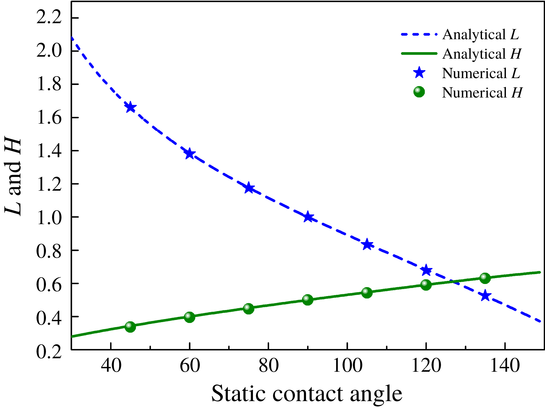Reference Cai, Marschall, Wörner and Deutschmann2014):

(4.1a,b ) $$\begin{eqnarray}L=2R_{0}\sqrt{\frac{\unicode[STIX]{x03C0}}{2(\unicode[STIX]{x1D703}_{s}-\sin \unicode[STIX]{x1D703}_{s}\cos \unicode[STIX]{x1D703}_{s})}}\sin \unicode[STIX]{x1D703}_{s},\quad H=R_{0}\sqrt{\frac{\unicode[STIX]{x03C0}}{2(\unicode[STIX]{x1D703}_{s}-\sin \unicode[STIX]{x1D703}_{s}\cos \unicode[STIX]{x1D703}_{s})}}(1-\cos \unicode[STIX]{x1D703}_{s}).\end{eqnarray}$$

We conduct several simulations in a wide range of surface wettability for both hydrophilic and hydrophobic cases ( $\unicode[STIX]{x1D703}_{s}$ varies from $45^{\circ }$ to $135^{\circ }$ ). Analytical and numerical values of $L$ and $H$ are compared in figure 2, and a good agreement is observed for all values of $\unicode[STIX]{x1D703}_{s}$ .

Figure 2.

Comparison of analytical and numerical values of spreading length $L$ and droplet height $H$ at different static contact angles $\unicode[STIX]{x1D703}_{s}$ . Here $\unicode[STIX]{x1D703}_{s}$ ranges from $45^{\circ }$ to $135^{\circ }$ with an interval $15^{\circ }$ .

To clearly demonstrate the effect of surfactants on the MCL, we compare the dynamics of clean and contaminated (with surfactants) droplets. The Langmuir adsorption constant $\unicode[STIX]{x1D713}_{c}$ and the parameter $Ex$ take values of 0.017 and 1, respectively, with the value of $Pi$ determined from (3.16). Other parameters are taken as before. Both hydrophilic ( $\unicode[STIX]{x1D703}_{s}=60^{\circ }$ ) and hydrophobic ( $\unicode[STIX]{x1D703}_{s}=120^{\circ }$ ) cases are considered in this study. For the contaminated droplet, the initialization of surfactant concentration is performed using the analytical prediction in (3.15) for $\unicode[STIX]{x1D713}$ with the initial surfactant bulk concentration $\unicode[STIX]{x1D713}_{b}=1.5\times 10^{-2}$ .

Figure 3.

Profiles of (a) contaminated droplet at different times and (b) clean and contaminated droplets in equilibrium on a hydrophilic surface with static contact angle $\unicode[STIX]{x1D703}_{s}=60^{\circ }$ . For the contaminated droplet, the initial surfactant bulk concentration $\unicode[STIX]{x1D713}_{b}$ is $1.5\times 10^{-2}$ . In (b), equilibrium contact angles $\unicode[STIX]{x1D703}_{e}$ for clean and contaminated droplets are $60^{\circ }$ and $52^{\circ }$ , respectively.

Figure 4.

Profiles of (a) contaminated droplet at different times and (b) clean and contaminated droplets in equilibrium on a hydrophobic surface with static contact angle $\unicode[STIX]{x1D703}_{s}=120^{\circ }$ . For the contaminated droplet, the initial surfactant bulk concentration $\unicode[STIX]{x1D713}_{b}$ is $1.5\times 10^{-2}$ . In (b), equilibrium contact angles for clean and contaminated droplets are $120^{\circ }$ and $129^{\circ }$ , respectively.

Figure 3(a) gives the evolution of a contaminated droplet on a hydrophilic surface at different times (t ranges from 0 to 10). The contaminated droplet constantly spreads until the steady state is reached. Equilibrium contact angles $\unicode[STIX]{x1D703}_{e}$ for clean and contaminated droplets in figure 3(b) are $60^{\circ }$ and $52^{\circ }$ , respectively. Obviously, the presence of surfactants makes the droplet more hydrophilic on a hydrophilic surface. In contrast to the hydrophilic surface, surfactants make the droplet more hydrophobic on a hydrophobic surface by increasing the equilibrium contact angle $\unicode[STIX]{x1D703}_{e}$ from $120^{\circ }$ to 129 $^{\circ }$ , as shown in figure 4. Results in figures 3 and 4 are consistent with the results obtained for sharp interface models (Lai et al. Reference Lai, Tseng and Huang2010; Xu & Ren Reference Xu and Ren2014; Zhang et al. Reference Zhang, Xu and Ren2014). We further calculate the spreading length $L$ , the droplet height $H$ and $\unicode[STIX]{x1D703}_{e}$ for the contaminated droplet ( $\unicode[STIX]{x1D713}_{b}=1.5\times 10^{-2}$ ) in a wide range of surface wettability ( $\unicode[STIX]{x1D703}_{s}$ varies from $45^{\circ }$ to $135^{\circ }$ ). Analytical $L$ and $H$ for the clean droplet in figure 5 serve as a comparison. It is observed from figure 5 that the effect of surfactants is more obvious on the strong hydrophilic or hydrophobic surface. The inset gives $\unicode[STIX]{x1D703}_{e}$ of the contaminated droplet. The blue line in the inset represents static contact angles $\unicode[STIX]{x1D703}_{s}$ of the clean droplet (the slope of this line is 1), and it serves as a reference. We found that $\unicode[STIX]{x1D703}_{e}$ can be approximately predicted by $\unicode[STIX]{x1D703}_{s}$ through a linear relationship: $\unicode[STIX]{x1D703}_{e}=1.3\unicode[STIX]{x1D703}_{s}-25.7$ .

Figure 5.

Numerical spreading length $L$ (points) and droplet height $H$ (points) for the contaminated droplet, and analytical values (lines) calculated from static contact angles serve as a comparison. For the contaminated droplet, the initial surfactant bulk concentration $\unicode[STIX]{x1D713}_{b}$ is $1.5\times 10^{-2}$ . The inset gives $\unicode[STIX]{x1D703}_{e}$ of the contaminated droplet. It can be observed that $\unicode[STIX]{x1D703}_{e}$ can be approximately predicted by $\unicode[STIX]{x1D703}_{s}$ through a linear relationship: $\unicode[STIX]{x1D703}_{e}=1.3\unicode[STIX]{x1D703}_{s}-25.7$ .

We also extend our work to a three-dimensional computational domain $[0,0.8]^{2}\times [0,0.4]$ . A grid size of $110^{2}\times 55$ and time step size $\unicode[STIX]{x1D6FF}t=8\times 10^{-4}$ are used in simulations. For the contaminated droplet, the initial surfactant bulk concentration $\unicode[STIX]{x1D713}_{b}$ is $2.5\times 10^{-2}$ . Results in figure 6 clearly demonstrate the effect of surfactants on the contact line dynamics. The presence of surfactants reduces $\unicode[STIX]{x1D703}_{e}$ from $60^{\circ }$ to $42^{\circ }$ on the hydrophilic surface, and increases $\unicode[STIX]{x1D703}_{e}$ from $120^{\circ }$ to $139^{\circ }$ on the hydrophobic surface.

Figure 6.

Profiles of clean and contaminated droplets on (a) hydrophilic ( $\unicode[STIX]{x1D703}_{s}=60^{\circ }$ ) and (b) hydrophobic ( $\unicode[STIX]{x1D703}_{s}=120^{\circ }$ ) surfaces. For the contaminated droplet, the initial surfactant bulk concentration $\unicode[STIX]{x1D713}_{b}$ is $2.5\times 10^{-2}$ . The computation domain is $[0,0.8]^{2}\times [0,0.4]$ . We use a grid size of $110^{2}\times 55$ and time step size $\unicode[STIX]{x1D6FF}t=8\times 10^{-4}$ in simulations. In (a), equilibrium contact angles $\unicode[STIX]{x1D703}_{e}$ of clean and contaminated droplets are $60^{\circ }$ and $42^{\circ }$ , respectively. In (b), equilibrium contact angles $\unicode[STIX]{x1D703}_{e}$ of clean and contaminated droplets are $120^{\circ }$ and $139^{\circ }$ , respectively.

Figure 7.

Evolutions of unbalanced Young stresses at right contact points of clean and contaminated droplets ( $\unicode[STIX]{x1D713}_{b}=1.5\times 10^{-2}$ ). The static contact angle $\unicode[STIX]{x1D703}_{s}$ of the hydrophilic surface is $60^{\circ }$ .

The Young equation can well explain the effect of surfactants on the droplet dynamics on the solid surface. As in Wang et al. (Reference Wang, Qian and Sheng2008), we can derive that

(4.2) $$\begin{eqnarray}\int _{int}[L\unicode[STIX]{x2202}_{\unicode[STIX]{x1D70F}}\unicode[STIX]{x1D719}]\,\text{d}\unicode[STIX]{x1D70F}=\int _{int}[\mathit{Cn}\unicode[STIX]{x2202}_{n}\unicode[STIX]{x1D719}\unicode[STIX]{x2202}_{\unicode[STIX]{x1D70F}}\unicode[STIX]{x1D719}+M^{\prime }(\unicode[STIX]{x1D719})\unicode[STIX]{x2202}_{\unicode[STIX]{x1D70F}}\unicode[STIX]{x1D719}]\,\text{d}\unicode[STIX]{x1D70F}=\unicode[STIX]{x1D70E}_{e}\cos \unicode[STIX]{x1D703}_{e}+\unicode[STIX]{x0394}\unicode[STIX]{x1D70E}_{fs},\end{eqnarray}$$

where $\int _{int}\text{d}\unicode[STIX]{x1D70F}$ denotes the integration across the fluid–fluid interface along the $\unicode[STIX]{x1D70F}$ -direction, $\unicode[STIX]{x0394}\unicode[STIX]{x1D70E}_{fs}$ is a function of the local composition at the solid surface measuring the fluid–solid interfacial free energy per unit area and $\unicode[STIX]{x1D70E}_{e}$ is the interfacial tension of a contaminated droplet in equilibrium. Equation (4.2) indicates that the unbalanced Young stress dominates the evolution of contact angle. It drives the droplet at two contact points to spread on a hydrophilic surface or to recoil on a hydrophobic surface. In equilibrium, the unbalanced Young stress decreases to zero (figure 7), namely $L=0$ , and (4.2) reduces to the classical Young equation

(4.3) $$\begin{eqnarray}\unicode[STIX]{x1D70E}_{e}\cos \unicode[STIX]{x1D703}_{e}+\unicode[STIX]{x0394}\unicode[STIX]{x1D70E}_{fs}=0.\end{eqnarray}$$

The boundary condition $\unicode[STIX]{x2202}_{n}\unicode[STIX]{x1D713}=0$ allows the presence of free surfactants on the fluid–solid interface, but these surfactants do not affect the fluid–solid interfacial tension through adsorption or the like, so clean and contaminated droplets have the same $\unicode[STIX]{x0394}\unicode[STIX]{x1D70E}_{fs}$ . Then we have

(4.4) $$\begin{eqnarray}\unicode[STIX]{x1D70E}_{e}\cos \unicode[STIX]{x1D703}_{e}=\unicode[STIX]{x1D70E}_{0}\cos \unicode[STIX]{x1D703}_{s},\end{eqnarray}$$

where $\unicode[STIX]{x1D70E}_{0}$ is the interfacial tension of a clean droplet. The addition of surfactants greatly reduces the interfacial tension between fluids, resulting in $\unicode[STIX]{x1D70E}_{e}<\unicode[STIX]{x1D70E}_{0}$ . We can derive that cos $\unicode[STIX]{x1D703}_{e}>\cos \unicode[STIX]{x1D703}_{s}$ from (4.4). Thus, $\unicode[STIX]{x1D703}_{e}$ is smaller than $\unicode[STIX]{x1D703}_{s}$ in the hydrophilic case (the contaminated droplet becomes more hydrophilic), and $\unicode[STIX]{x1D703}_{e}$ is larger than $\unicode[STIX]{x1D703}_{s}$ in the hydrophobic case (the contaminated droplet becomes more hydrophobic).

We denote the unbalanced Young stresses at right contact points of clean and contaminated droplets as $F_{Rc}$ and $F_{Rs}$ , respectively. Figure 7 gives evolutions of $F_{Rc}$ and $F_{Rs}$ , and the whole process can be divided into three stages. In the first stage, the contaminated droplet spreads faster than the clean droplet since $F_{Rs}$ is larger than $F_{Rc}$ . During the droplet spreading process, the unbalanced Young stress always drags the right contact point forward to reduce the contact angle, and it decreases as the contact angle changes until equilibrium. Thus, to some extent, the unbalanced Young stress can be reflected in the contact angle. Obviously, at the same moment, the contaminated droplet has a smaller contact angle than the clean droplet, which explains why the change in $F_{Rs}$ is more dramatic in the second stage. It can be observed that $F_{Rs}$ is larger than $F_{Rc}$ in the third stage, and this fact may account for a smaller equilibrium contact angle of the contaminated droplet.

Figure 8.

The linear relationship between the interfacial tension lowering $\unicode[STIX]{x0394}\unicode[STIX]{x1D70E}/\unicode[STIX]{x1D70E}_{0}$ and $\ln (1-\unicode[STIX]{x1D713}_{0})$ . Fitted formulas of green and blue lines can be approximated as $\unicode[STIX]{x0394}\unicode[STIX]{x1D70E}/\unicode[STIX]{x1D70E}_{0}=0.3396\ln (1-\unicode[STIX]{x1D713}_{0})$ and $\unicode[STIX]{x0394}\unicode[STIX]{x1D70E}/\unicode[STIX]{x1D70E}_{0}=0.1942\ln (1-\unicode[STIX]{x1D713}_{0})$ , respectively. These results directly validate the equilibrium equation of state (3.18).

The interfacial tension lowering $\unicode[STIX]{x0394}\unicode[STIX]{x1D70E}$ of a contaminated droplet in equilibrium can be calculated from

(4.5) $$\begin{eqnarray}\unicode[STIX]{x0394}\unicode[STIX]{x1D70E}=\unicode[STIX]{x1D70E}_{e}-\unicode[STIX]{x1D70E}_{0}=\unicode[STIX]{x1D70E}_{0}\left(\frac{\cos \unicode[STIX]{x1D703}_{s}-\cos \unicode[STIX]{x1D703}_{e}}{\cos \unicode[STIX]{x1D703}_{e}}\right).\end{eqnarray}$$

Now we perform a series of numerical experiments to verify the linear relationship between $\unicode[STIX]{x0394}\unicode[STIX]{x1D70E}$ and ln(1– $\unicode[STIX]{x1D713}_{0}$ ) analytically obtained in (3.18). Two different scenarios are considered in this study: $Ex=0.5$ and $Ex=1$ . In each scenario, we conduct simulations with different surfactant bulk concentrations, e.g. $\unicode[STIX]{x1D713}_{b}=1\times 10^{-2}$ , $1.5\times 10^{-2}$ and $2\times 10^{-2}$ . The static contact angle $\unicode[STIX]{x1D703}_{s}$ of the bottom surface is taken to be $60^{\circ }$ . From the resulting profile of surfactant concentration in equilibrium, the surfactant loading of interface $\unicode[STIX]{x1D713}_{0}$ can be directly obtained. The equilibrium contact angle $\unicode[STIX]{x1D703}_{e}$ can be easily calculated when the contaminated droplet reaches the steady state, and then we get the interfacial tension lowering $\unicode[STIX]{x0394}\unicode[STIX]{x1D70E}$ from (4.5). Obviously, there is a linear relationship between $\unicode[STIX]{x0394}\unicode[STIX]{x1D70E}$ and $\ln (1-\unicode[STIX]{x1D713}_{0})$ , as plotted in figure 8, which directly validates the equilibrium equation of state (3.18). We use linear formulas to fit simulated values at different $Ex$ , and fitted equations of green and blue lines can be approximated as $\unicode[STIX]{x0394}\unicode[STIX]{x1D70E}/\unicode[STIX]{x1D70E}_{0}=0.3396\ln (1-\unicode[STIX]{x1D713}_{0})$ and $\unicode[STIX]{x0394}\unicode[STIX]{x1D70E}/\unicode[STIX]{x1D70E}_{0}=0.1942\ln (1-\unicode[STIX]{x1D713}_{0})$ , respectively. It worth noting that $Ex$ plays an important role in reducing the interfacial tension, and its effect is more obvious at higher interfacial surfactant concentration. We infer, in the last part of § 3, that the coefficient $k$ is determined by $Ex$ for the given Langmuir adsorption constant $\unicode[STIX]{x1D713}_{c}$ and interfacial thickness $Cn$ . It can be observed that the slopes ( $kPi$ ) of two fitted curves in figure 8 equal $0.1942$ ( $Ex=1$ ) and $0.3396$ ( $Ex=0.5$ ), respectively. The dimensionless parameter $Pi$ can be calculated from (3.16). Then we can obtain that $k$ equals 1.05 and 1.11 for the cases of $Ex=1$ and $Ex=0.5$ , respectively. This result verifies our inference that $k$ depends on $Ex$ .

Figure 9.

The relative interfacial tension $\unicode[STIX]{x1D70E}_{e}/\unicode[STIX]{x1D70E}_{0}$ at different surfactant bulk concentrations $\unicode[STIX]{x1D713}_{b}$ . The Langmuir adsorption constant $\unicode[STIX]{x1D713}_{c}$ is 0.017. The analytical equation (4.6) fits the simulated values very well.

Using the Langmuir isotherm in (3.15) and equilibrium equation of state (3.18), we obtain the relationship between the relative interfacial tension $\unicode[STIX]{x1D70E}_{e}/\unicode[STIX]{x1D70E}_{0}$ and surfactant bulk concentration $\unicode[STIX]{x1D713}_{b}$ :

(4.6) $$\begin{eqnarray}\frac{\unicode[STIX]{x1D70E}_{e}}{\unicode[STIX]{x1D70E}_{0}}=-\frac{kPi}{\unicode[STIX]{x1D70E}_{0}}\ln (\unicode[STIX]{x1D713}_{b}+\unicode[STIX]{x1D713}_{c})+\frac{kPi}{\unicode[STIX]{x1D70E}_{0}}\ln \unicode[STIX]{x1D713}_{c}+1,\end{eqnarray}$$

where the Langmuir adsorption constant $\unicode[STIX]{x1D713}_{c}$ is 0.017 in this study. It can be observed that (4.6) fits the simulated values very well in figure 9, indicating the correctness of the Langmuir isotherm and the equilibrium equation of state to some extent. Again, we can see that the coefficient $k$ is determined by $Ex$ .

4.2 Droplet dynamics on a chemically patterned surface

4.2.1 Phase diagram of flow states

Having validated the MCL model, we investigate the droplet dynamics with soluble surfactants on a chemically patterned surface. The computational domain is $\unicode[STIX]{x1D6FA}=[0,4]\times [0,1]$ with periodic boundary conditions applied on the horizontal direction, as shown in figure 10. Initially, a semicircular droplet with a radius of 0.5 is placed on the bottom surface with static contact angles $\unicode[STIX]{x1D703}_{1}$ ( $\unicode[STIX]{x1D703}_{1}<90^{\circ }$ ) for the hydrophilic A-type stripe and $\unicode[STIX]{x1D703}_{2}$ ( $\unicode[STIX]{x1D703}_{2}>90^{\circ }$ ) for the hydrophobic B-type stripe. The droplet centre is located at (1, 0). A constant body force along the horizontal direction is applied on the droplet. A grid size of $600\times 150$ and time step size $\unicode[STIX]{x1D6FF}t=5\times 10^{-4}$ are used in all simulations. The Reynolds number $Re$ and Péclet numbers $Pe_{\unicode[STIX]{x1D719}}$ and $Pe_{\unicode[STIX]{x1D713}}$ are taken as 20, 100 and 10, respectively. The value of Cahn number $Cn$ is 0.01. The relaxation parameter $Pe_{\mathit{s}}$ and slip length $L_{s}$ are set to 0.005 and 0.0038, respectively. Both density ratio $\unicode[STIX]{x1D706}_{\unicode[STIX]{x1D70C}}$ and viscosity ratio $\unicode[STIX]{x1D706}_{\unicode[STIX]{x1D708}}$ of the droplet to the surrounding fluid are 2. The initial surfactant bulk concentration $\unicode[STIX]{x1D713}_{b}$ is $1.5\times 10^{-2}$ . To clearly demonstrate the effect of surfactants, we compare the dynamics of clean and contaminated droplets.

Figure 10.

Schematic of computation domain $\unicode[STIX]{x1D6FA}=[0,L]\times [0,H]$ . A semicircular droplet with a radius of $L/8$ is placed on a chemically patterned surface with static contact angles $\unicode[STIX]{x1D703}_{1}$ ( $\unicode[STIX]{x1D703}_{1}<90^{\circ }$ ) for the hydrophilic A-type stripe (black stripe) and $\unicode[STIX]{x1D703}_{2}$ ( $\unicode[STIX]{x1D703}_{2}>90^{\circ }$ ) for the hydrophobic B-type stripe (green stripe). The droplet centre is located at ( $L/4,0$ ). The droplet is pushed along the horizontal direction by a constant body force.

Figure 11.

Dynamics of clean (blue) and contaminated (red) droplets on a chemically patterned surface with static contact angles $\unicode[STIX]{x1D703}_{1}=60^{\circ }$ for the A-type stripe (black stripe) and $\unicode[STIX]{x1D703}_{2}=120^{\circ }$ for the B-type stripe (green stripe). Droplets are pushed by a constant body force along the horizontal direction.

Figure 12.

Evolution of the surfactant concentration for a contaminated droplet. The initial surfactant bulk concentration $\unicode[STIX]{x1D713}_{b}$ is $1.5\times 10^{-2}$ .

Figure 11 gives the evolution of droplets on a chemically patterned surface. At first, both clean and contaminated droplets spread out over the hydrophilic surface due to the unbalanced Young stress, and then move forward under the action of a constant body force (figure 11 b). After crossing the junction of wettability transition, both droplets suffer from large deformation and break up into daughter droplets. Obviously, compared with the clean droplet, the contaminated droplet has a larger advancing angle on the hydrophobic B-type stripe and a smaller receding angle on the hydrophilic A-type stripe (figure 11 c). We also note that the break-up of the contaminated droplet occurs earlier than that of the clean droplet (figure 11 d). After the break-up, the spreading droplets left on the hydrophobic stripe begin to contract (figure 11 e). Subsequently, daughter droplets detached from the solid surface move towards daughter droplets in contact with the B-type stripe (figure 11 f). As two clean daughter droplets approach each other, the film between them becomes very thin, and then they merge together due to the effect of interfacial tension. The merging droplet continues to slide on the hydrophilic A-type stripe (figure 11 j). While the thin film between two contaminated daughter droplets is always maintained at a certain thickness until they slide over each other (figure 11 h). Note that both contaminated daughter droplets eventually detach from the bottom surface. Figure 12 shows the evolution of surfactant concentration. The surfactant concentration around the interface is much larger than that for other regions, and the distribution of surfactants is non-uniform along the interface. In fact, the different behaviour between contaminated and clean droplets is caused by (1) the uniform reduction of interfacial tension and (2) the non-uniform effects from the non-uniform interfacial tension and the Marangoni stress along the interface. We also see that surfactants are swept into the bulk phases when concentration reaches a maximum at the droplet tip (figure 12 e). Figure 13 presents the evolutions of pressure field and surfactant concentration during the collision of two contaminated droplets. It can be observed that the pressure in the gap between two contaminated droplets increases significantly as they approach each other (point A to point C). The increasing pressure pushes surfactants away from the near-contact region, and the resulting Marangoni force acts as a repulsive force to prevent droplet coalescence (Liu & Zhang Reference Liu and Zhang2010; Wodlei et al. Reference Wodlei, Sebilleau, Magnaudet and Pimienta2018). The pressure in the gap decreases (point D to point E) as two contaminated droplets slide over each other.

Figure 13.

Evolutions of (a) pressure field (background colour), (b) surfactant concentration and (c) pressure during the separation of two contaminated droplets. The initial surfactant bulk concentration $\unicode[STIX]{x1D713}_{b}$ is $1.5\times 10^{-2}$ .

There are several parameters that potentially influence the dynamics of a contaminated droplet on a chemically patterned surface, e.g. the surfactant bulk concentration $\unicode[STIX]{x1D713}_{b}$ , the defect strength $\unicode[STIX]{x0394}\unicode[STIX]{x1D703}_{e}=\unicode[STIX]{x1D703}_{2}-\unicode[STIX]{x1D703}_{1}$ , the Reynolds number $Re$ , etc. In this work, we only consider the effect of $\unicode[STIX]{x1D713}_{b}$ and $\unicode[STIX]{x0394}\unicode[STIX]{x1D703}_{e}$ on the behaviour of a contaminated droplet. A series of numerical simulations, with $\unicode[STIX]{x1D713}_{b}$ ranging from $1\times 10^{-3}$ to $1.5\times 10^{-2}$ and $\unicode[STIX]{x0394}\unicode[STIX]{x1D703}_{\mathit{e}}$ ranging from $20^{\circ }$ to $100^{\circ }$ , are conducted to obtain a clear understanding of the droplet dynamics. Other parameters and boundary conditions remain unchanged. Results demonstrate that all contaminated droplets at various conditions suffer from large deformation and break-up, just as in figure 11(c,d). After droplet break-up, we observe three typical flow states, specifically the coalescence mode, the non-coalescence mode and the detachment mode, as shown in figure 14. At low $\unicode[STIX]{x1D713}_{b}$ and medium $\unicode[STIX]{x0394}\unicode[STIX]{x1D703}_{e}$ ( $\unicode[STIX]{x1D713}_{b}=1\times 10^{-3}$ and $\unicode[STIX]{x0394}\unicode[STIX]{x1D703}_{e}=70^{\circ }$ ), the coalescence occurs as two contaminated droplets move towards each other because of the interfacial tension. At high $\unicode[STIX]{x1D713}_{b}$ and low $\unicode[STIX]{x0394}\unicode[STIX]{x1D703}_{e}$ ( $\unicode[STIX]{x1D713}_{b}=1.5\times 10^{-2}$ and $\unicode[STIX]{x0394}\unicode[STIX]{x1D703}_{e}=50^{\circ }$ ), the repulsive Marangoni force together with the low interfacial tension leads to the separation of two daughter droplets, and the droplet in contact with the bottom wall will continue to slide on the hydrophilic A-type stripe. This phenomenon is called ‘non-coalescence’. If we increase $\unicode[STIX]{x0394}\unicode[STIX]{x1D703}_{e}$ on the basis of the non-coalescence event ( $\unicode[STIX]{x1D713}_{b}=1.5\times 10^{-2}$ and $\unicode[STIX]{x0394}\unicode[STIX]{x1D703}_{e}=70^{\circ }$ ), the detachment event will occur, when the droplet sliding on the bottom wall (green stripe) leaves the patterned surface. Note that the droplet can only detach from the solid surface on the hydrophobic B-type stripe (green stripe).

Figure 14.

Three typical flow states of contaminated droplets at various surfactant bulk concentrations $\unicode[STIX]{x1D713}_{b}$ and defect strengths $\unicode[STIX]{x0394}\unicode[STIX]{x1D703}_{e}$ : coalescence, non-coalescence and detachment. The A-type stripe (black stripe) with static contact angle $\unicode[STIX]{x1D703}_{1}$ is hydrophilic and the B-type stripe (green stripe) with static contact angle $\unicode[STIX]{x1D703}_{2}$ is hydrophobic. We define the defect strength $\unicode[STIX]{x0394}\unicode[STIX]{x1D703}_{e}$ as the difference of $\unicode[STIX]{x1D703}_{1}$ and $\unicode[STIX]{x1D703}_{2}$ , namely $\unicode[STIX]{x0394}\unicode[STIX]{x1D703}_{e}=\unicode[STIX]{x1D703}_{2}-\unicode[STIX]{x1D703}_{1}$ .

A phase diagram of flow states for contaminated droplets at different $\unicode[STIX]{x1D713}_{b}$ and $\unicode[STIX]{x0394}\unicode[STIX]{x1D703}_{e}$ is further shown in figure 15. A black star identifies a coalescence event, a red diamond marks a non-coalescence event and a blue circle represents a detachment event. As we can see, only non-coalescence occurs for all $\unicode[STIX]{x1D713}_{b}$ when $\unicode[STIX]{x0394}\unicode[STIX]{x1D703}_{e}$ is less than $60^{\circ }$ . The surfactant bulk concentration $\unicode[STIX]{x1D713}_{b}$ begins to affect the flow state of a droplet as the defect strength $\unicode[STIX]{x0394}\unicode[STIX]{x1D703}_{e}$ increases to $60^{\circ }$ . Detachment events occur at high $\unicode[STIX]{x1D713}_{b}$ since surfactants reduce the adsorption effect of the B-type stripe by increasing advancing contact angles of droplets. With a decrease of $\unicode[STIX]{x1D713}_{b}$ , droplets cannot detach from the B-type stripe due to the weak effect of surfactants, and non-coalescence phenomena appear. If we further reduce $\unicode[STIX]{x1D713}_{b}$ , a large interfacial tension will lead to the coalescence of two contaminated droplets. It can be observed that non-coalescence events occur on a narrower range of $\unicode[STIX]{x1D713}_{b}$ at $\unicode[STIX]{x0394}\unicode[STIX]{x1D703}_{e}=70^{\circ }$ and completely disappear when $\unicode[STIX]{x0394}\unicode[STIX]{x1D703}_{e}$ is larger than $70^{\circ }$ . Detachment and coalescence events dominate flow states of droplets at $\unicode[STIX]{x0394}\unicode[STIX]{x1D703}_{e}=80^{\circ }$ . Coalescence events only occur at specific surfactant bulk concentrations when $\unicode[STIX]{x0394}\unicode[STIX]{x1D703}_{e}$ is larger than $80^{\circ }$ . Overall, the non-coalescence event is the only flow state of contaminated droplets at low defect strength ( $\unicode[STIX]{x0394}\unicode[STIX]{x1D703}_{e}\leqslant 50^{\circ }$ ) and completely disappears at high defect strength ( $\unicode[STIX]{x0394}\unicode[STIX]{x1D703}_{e}\geqslant 80^{\circ }$ ). All three flow states occur at medium defect strength ( $50^{\circ }<\unicode[STIX]{x0394}\unicode[STIX]{x1D703}_{e}<80^{\circ }$ ). The detachment event dominates the flow behaviour of droplets at high defect strength.

Figure 15.

A phase diagram of flow states for contaminated droplets at different surfactant bulk concentrations $\unicode[STIX]{x1D713}_{b}$ and defect strengths $\unicode[STIX]{x0394}\unicode[STIX]{x1D703}_{e}$ . A black star identifies a coalescence event, a red diamond marks a non-coalescence event and a blue circle represents a detachment event.

4.2.2 Unbalanced Young stress at the MCL

In this section, we focus on the evolution of the unbalanced Young stress $L\unicode[STIX]{x2202}_{\unicode[STIX]{x1D70F}}\unicode[STIX]{x1D719}$ when a contaminated droplet moves across the junction of wettability transition. As a contaminated droplet moves along the $x$ direction, the advancing contact angle and receding contact angle are denoted as $\unicode[STIX]{x1D703}_{A}$ and $\unicode[STIX]{x1D703}_{R}$ , respectively. Stresses $F_{A}$ and $F_{R}$ are unbalanced Young stresses acting on the triple-phase contact points A and R, respectively. As shown in figure 16, the unbalanced Young stress is defined as positive when it points from left to right; otherwise, it is defined as negative. We calculate unbalanced Young stresses $F_{A}$ and $F_{R}$ within the time range 0–2.8, and details of droplet dynamics in this period are depicted in figure 11(a–c). During the process, the triple-phase contact point A moves from the hydrophilic A-type stripe to the hydrophobic B-type stripe, while the point R never crosses the junction.

Figure 16.

Illustration of unbalanced Young stresses $F_{A}$ and $F_{R}$ at the triple-phase contact points A and R. Angle $\unicode[STIX]{x1D703}_{A}$ is the advancing contact angle and $\unicode[STIX]{x1D703}_{R}$ is the receding contact angle.

Figure 17.

Evolutions of unbalanced Young stresses (a) $F_{R}$ and (b)  $F_{A}$ at different defect strengths $\unicode[STIX]{x0394}\unicode[STIX]{x1D703}_{e}$ . The initial surfactant bulk concentration $\unicode[STIX]{x1D713}_{b}$ is $1.5\times 10^{-2}$ .

The chemical potential $L$ in the unbalanced Young stress measures the deviation from the equilibrium condition ( $L=0$ ) at the solid surface, and the main role of the unbalanced Young stress is to adjust the droplet to its equilibrium condition (equilibrium contact angle $\unicode[STIX]{x1D703}_{e}$ ). Figure 17 gives the evolutions of unbalanced Young stresses $F_{R}$ and $F_{A}$ . Initially, the static droplet ( $\unicode[STIX]{x1D703}_{0}=90^{\circ }$ ) spreads on the hydrophilic surface under the action of $F_{R}$ and $F_{A}$ . Stress $F_{R}$ points to the left (negative) and $F_{A}$ points in the opposite direction (positive). Both $F_{R}$ and $F_{A}$ decrease dramatically as $\unicode[STIX]{x1D703}_{R}$ and $\unicode[STIX]{x1D703}_{A}$ approach the equilibrium contact angle $\unicode[STIX]{x1D703}_{e}$ ( $\unicode[STIX]{x1D703}_{e}<\unicode[STIX]{x1D703}_{s}$ on a hydrophilic surface). Meanwhile, the droplet keeps deforming as a constant body force drives it forward. The receding contact angle $\unicode[STIX]{x1D703}_{R}$ decreases with the deformation of the droplet, and $F_{R}$ becomes zero when $\unicode[STIX]{x1D703}_{R}$ decreases to $\unicode[STIX]{x1D703}_{e}$ , as shown in figure 17(a). The continuous deformation of the droplet causes the receding contact angle $\unicode[STIX]{x1D703}_{R}$ to continue to decrease ( $\unicode[STIX]{x1D703}_{R}<\unicode[STIX]{x1D703}_{e}$ ). In order to adjust the contact point R to the equilibrium condition, $F_{R}$ changes its direction (now it points to the right, positive) and pushes the contact point R to move forward. During the whole process, the contact point R never moves across the junction of wettability transition.

The evolution of $F_{A}$ is more complicated than that of $F_{R}$ . Before $\unicode[STIX]{x1D703}_{A}$ decreases to the equilibrium contact angle $\unicode[STIX]{x1D703}_{e}$ , droplet deformation leads to an increase of $\unicode[STIX]{x1D703}_{A}$ , which is contrary to the expectation of $F_{A}$ . Thus, $F_{A}$ begins to increase (point M in figure 17 b) and drags the contact point A forward to reduce $\unicode[STIX]{x1D703}_{A}$ . As the contact point A meets the junction, $F_{A}$ experiences a dramatic decrease (point N). According to the GNBC, the dectrease of $F_{A}$ must be accompanied by the decrease of fraction force due to the contact line slip. Thus, the classical phenomenon of the contact line sticking to the solid surface is expected to occur at the point N, and this is actually observed in figure 18.

Figure 18.

Profiles of phase-field variable $\unicode[STIX]{x1D719}$ at different times. The initial surfactant bulk concentration $\unicode[STIX]{x1D713}_{b}$ is $1.5\times 10^{-2}$ .

In figure 17(b), we can see that the defect strength $\unicode[STIX]{x0394}\unicode[STIX]{x1D703}_{e}$ has a significant impact on the behaviour of $F_{A}$ . When the defect strength $\unicode[STIX]{x0394}\unicode[STIX]{x1D703}_{e}$ is less than $80^{\circ }$ , $\unicode[STIX]{x1D703}_{A}$ immediately arrives at the equilibrium contact angle $\unicode[STIX]{x1D703}_{e}$ of the hydrophobic B-type stripe. With droplet deformation, $\unicode[STIX]{x1D703}_{A}$ continues to increase and exceeds $\unicode[STIX]{x1D703}_{e}$ , and correspondingly $F_{A}$ increases to reduce $\unicode[STIX]{x1D703}_{A}$ . Throughout the whole process, $F_{A}$ never changes direction, and always drags the contact point A forward. The behaviour of $F_{A}$ becomes complicated when $\unicode[STIX]{x0394}\unicode[STIX]{x1D703}_{e}$ is larger than $80^{\circ }$ . As the droplet moves across the junction, $\unicode[STIX]{x1D703}_{A}$ ( $\unicode[STIX]{x1D703}_{A}<90^{\circ }$ ) is less than $\unicode[STIX]{x1D703}_{e}$ ( $\unicode[STIX]{x1D703}_{e}>90^{\circ }$ on a hydrophobic surface). In order to adjust $\unicode[STIX]{x1D703}_{A}$ , the unbalanced Young stress $F_{A}$ , acting as the drag force before (positive), decreases dramatically and changes its direction (negative). Stress $F_{A}$ decreases to zero when $\unicode[STIX]{x1D703}_{A}$ arrives at $\unicode[STIX]{x1D703}_{e}$ , and it becomes the drag force again as $\unicode[STIX]{x1D703}_{A}$ exceeds $\unicode[STIX]{x1D703}_{e}$ with droplet deformation. Based on the above analysis, we can conclude that the unbalanced Young stress could be a driving or resistance force, which is determined by the critical defect strength $\unicode[STIX]{x0394}\unicode[STIX]{x1D703}_{e}$ , and $\unicode[STIX]{x0394}\unicode[STIX]{x1D703}_{e}$ is between $60^{\circ }$ and $80^{\circ }$ .