

1 Introduction
The two similarity hypotheses of Kolmogorov (Reference Kolmogorov1941a) and his derivation of the  $4/5$ law (Kolmogorov Reference Kolmogorov1941b) – these two papers will henceforth be referred to as K41 – have had a major impact on small-scale turbulence research. Kolmogorov’s (Kolmogorov Reference Kolmogorov1962) refined similarity hypothesis, or K62, has also had a considerable impact on small-scale turbulence research, albeit for different reasons.
It is now recognized that K41 and K62 represent in fact diametrically opposite views of the physics underpinning small-scale turbulence. In K41, the small scales are assumed to be completely immune from the influence of the large scales, with the underlying assumption that the Reynolds number is extremely, if not infinitely, large and the small scales are homogeneous and isotropic. This scenario is consistent with the  $4/5$ law since its derivation requires that the effect of viscosity and the influence of the large scales are negligible. In particular, the neglect of the non-stationary, in effect the large-scale, term in the Kármán–Howarth (e.g. Antonia et al. Reference Antonia, Tang, Djenidi and Zhou2019) equation is only justifiable when the Reynolds number is infinitely large; if one associates the
 $4/5$ law with the establishment of an inertial range (IR), then the latter is only a meaningful concept for infinitely large Reynolds numbers.
Like K41, K62 also assumes that the Reynolds number is very large. However, it proposes correcting for the non-stationarity of  $\overline{\unicode[STIX]{x1D716}}$, the mean energy dissipation rate, by explicitly accounting for the effect of the large scales. The K41 similarity based on
 $\overline{\unicode[STIX]{x1D716}}$ is now replaced by a similarity based on
 $\unicode[STIX]{x1D716}_{r}$, or energy dissipation averaged over a local volume of characteristic dimensions. K62 further assumes that the
 $4/5$ law is unaffected. This is inconsistent with the derivation of the
 $4/5$ law (Antonia et al. Reference Antonia, Tang, Djenidi and Zhou2019) which requires the effect of the large scales to be negligible.
K62 used a log-normal model for  $\unicode[STIX]{x1D716}_{r}$, first introduced by Obukhov (Reference Obukhov1962) to account for the slow and large-scale variation of
 $\overline{\unicode[STIX]{x1D716}}$ in the atmospheric surface layer. According to this model, the variance
 $\unicode[STIX]{x1D70E}^{2}$ of
 $\ln \unicode[STIX]{x1D716}_{r}$ in the IR is given by
 $$\begin{eqnarray}\unicode[STIX]{x1D70E}^{2}=A+\unicode[STIX]{x1D707}\ln \frac{L}{r}\;(r\ll L),\end{eqnarray}$$
where  $\unicode[STIX]{x1D707}$ is the intermittency exponent, or sometimes intermittency correction,
 $L$ is an external or integral length scale (it is defined in § 2) and
 $A$ is a constant that may depend on the macrostructure of the flow. K62 uses (1.1) to suggest that all moments of
 $\unicode[STIX]{x1D6FF}u\equiv u(x+r)-u(x)$, except for
 $\overline{(\unicode[STIX]{x1D6FF}u)^{3}}$, should be modified, relative to K41, as follows
 $$\begin{eqnarray}\overline{(\unicode[STIX]{x1D6FF}u)^{n}}\sim (\overline{\unicode[STIX]{x1D716}}r)^{n/3}\left(\frac{L}{r}\right)^{(\unicode[STIX]{x1D707}n(n-3))/18},\end{eqnarray}$$
where  $u$ is the velocity fluctuation and
 $r$ is a spatial increment. Some rationale for the log-normal model was provided by Yaglom (Reference Yaglom1966), Gurvich & Yaglom (Reference Gurvich and Yaglom1967) and Monin & Yaglom (Reference Monin and Yaglom1975) who used a mathematical description of the energy cascade to conclude that any non-negative quantity associated with the fine-scale structure has a probability density function that is approximately log-normal with a variance similar to that given by (1.1). In particular, these authors showed, by assuming self-similarity in the IR, that the averaged value of the product
 $\overline{\unicode[STIX]{x1D716}(x)\unicode[STIX]{x1D716}(x+r)}$ is given by
 $$\begin{eqnarray}\unicode[STIX]{x1D6F9}(r)=\frac{\overline{\unicode[STIX]{x1D716}(x)\unicode[STIX]{x1D716}(x+r)}}{\overline{\unicode[STIX]{x1D716}}^{2}}=D\left(\frac{L}{r}\right)^{\unicode[STIX]{x1D707}},\end{eqnarray}$$
where  $D$ (
 $\equiv e^{A}$) may depend on the flow macrostructure.
All of the above relations apply at very large Reynolds numbers. When the Reynolds number is finite, the Kármán–Howarth equation can admit similarity based on  $\overline{\unicode[STIX]{x1D716}}$ and
 $\unicode[STIX]{x1D708}$, the kinematic viscosity of the fluid, provided
 $r$ is small so that the effect of the large scales can be discounted (Antonia, Djenidi & Danaila Reference Antonia, Djenidi and Danaila2014). There is overwhelming support for this idea in the literature (e.g. Antonia et al. Reference Antonia, Djenidi, Danaila and Tang2017; Djenidi, Antonia & Tang Reference Djenidi, Antonia and Tang2019; Tang et al. Reference Tang, Antonia, Djenidi and Zhou2019); in general, statistics of small-scale fluctuations in the dissipative range scale on
 $\overline{\unicode[STIX]{x1D716}}$ and
 $\unicode[STIX]{x1D708}$, implying that the very large Reynolds number requirement of the first similarity hypothesis of K41 can be relaxed considerably. Quantities such as the skewness and flatness factor of
 $\unicode[STIX]{x2202}u/\unicode[STIX]{x2202}x$ can become independent of
 $Re_{\unicode[STIX]{x1D706}}$, the Taylor microscale Reynolds number defined by
 $u^{\prime }\unicode[STIX]{x1D706}/\unicode[STIX]{x1D708}$, where
 $\unicode[STIX]{x1D706}$ is the longitudinal Taylor microscale defined by
 $\unicode[STIX]{x1D706}=u^{\prime }/(\unicode[STIX]{x2202}u/\unicode[STIX]{x2202}x)^{\prime }$ and a prime denotes a root-mean-square value, provided
 $Re_{\unicode[STIX]{x1D706}}$ is sufficiently large.
The precise value of  $Re_{\unicode[STIX]{x1D706}}$ will depend on the flow (e.g. Antonia et al. Reference Antonia, Tang, Djenidi and Danaila2015; Tang et al. Reference Tang, Antonia, Djenidi, Abe, Zhou, Danaila and Zhou2015a,Reference Tang, Antonia, Djenidi and Zhoub, Reference Tang, Antonia, Djenidi, Danaila and Zhou2018) since the large-scale structure may differ in different flows. The situation is rather different as
 $r$ increases beyond the dissipation range. Quantities such as
 $\overline{(\unicode[STIX]{x1D6FF}u^{\ast })^{n}}$, where the asterisk denotes normalization by the Kolmogorov length scale
 $\unicode[STIX]{x1D702}\equiv (\unicode[STIX]{x1D708}^{3}/\overline{\unicode[STIX]{x1D716}})^{1/4}$ and the Kolmogorov velocity scale
 $u_{K}\equiv (\unicode[STIX]{x1D708}\overline{\unicode[STIX]{x1D716}})^{1/4}$, continue to evolve with
 $Re_{\unicode[STIX]{x1D706}}$, reflecting the importance of the finite Reynolds number, or FRN, effect (Qian Reference Qian1997, Reference Qian1998; Antonia & Burattini Reference Antonia and Burattini2006; Tchoufag, Sagaut & Cambon Reference Tchoufag, Sagaut and Cambon2012; Tang et al. Reference Tang, Antonia, Djenidi, Danaila and Zhou2017, Reference Tang, Antonia, Djenidi and Zhou2019). This raises a serious concern as to whether the IR, in the context of
 $\overline{(\unicode[STIX]{x1D6FF}u^{\ast })^{n}}$, can exist at finite Reynolds numbers and hence whether the exponent of
 $r$ in (1.2) can be defined without ambiguity even when
 $n$ is equal to 2 or 3. And yet, the power-law behaviour of (1.3) has been observed (e.g. Monin & Yaglom Reference Monin and Yaglom1975; Nelkin Reference Nelkin1981; Antonia, Satyaprakash & Hussain Reference Antonia, Satyaprakash and Hussain1982; Kuznetsov, Praskovsky & Sabelnikov Reference Kuznetsov, Praskovsky and Sabelnikov1992; Sreenivasan & Kailasnath Reference Sreenivasan and Kailasnath1993; Praskovsky & Oncley Reference Praskovsky and Oncley1994; Sreenivasan & Antonia Reference Sreenivasan and Antonia1997; Cleve, Greiner & Sreenivasan Reference Cleve, Greiner and Sreenivasan2003; Cleve et al. Reference Cleve, Greiner, Pearson and Sreenivasan2004) and the value of
 $\unicode[STIX]{x1D707}$ (
 ${\approx}0.2$) has, allowing for experimental uncertainties, been reproduced fairly convincingly in various flows.
It would seem that a quantity such as  $\unicode[STIX]{x1D6F9}$, which is more closely associated with small scales than
 $\unicode[STIX]{x1D6FF}u(r)$ at a comparable value of
 $r$, can exhibit a power law at relatively moderate Reynolds numbers even though
 $\overline{(\unicode[STIX]{x1D6FF}u)^{n}}$ has yet to exhibit a convincing power law and hence an IR. Since the relationship between the power-law range for
 $\unicode[STIX]{x1D6F9}$ and the IR, which requires
 $Re_{\unicode[STIX]{x1D706}}$ to be very large (Antonia et al. Reference Antonia, Tang, Djenidi and Zhou2019), is unclear at this stage, we will, for clarity, refer to the range over which
 $\unicode[STIX]{x1D6F9}$ behaves like
 $r^{-\unicode[STIX]{x1D707}}$ as the ‘power-law’ range. To the best of our knowledge, the focus to date has been on inferring the exponent
 $\unicode[STIX]{x1D707}$, equation (1.3), from the power-law range of
 $\unicode[STIX]{x1D6F9}(r)$ rather than on enquiring whether the similarity based on
 $L$, a concept fundamental to K62, is in fact valid. This is somewhat surprising since it is by no means certain that
 $\unicode[STIX]{x1D6F9}$ will exhibit a similarity based on
 $r/L$. Djenidi et al. (Reference Djenidi, Antonia and Tang2019) showed by plotting data for
 $\overline{(\unicode[STIX]{x1D6FF}u)^{2}}/\overline{u^{2}}$ versus
 $r/L$ that there is no collapse over what is loosely referred to in the literature as the scaling range; we stress, however, that quantities like
 $\overline{(\unicode[STIX]{x1D6FF}u)^{2}}$ and
 $\overline{(\unicode[STIX]{x1D6FF}u)^{3}}$ do not exhibit a power-law behaviour over this range (Antonia et al. Reference Antonia, Tang, Djenidi and Zhou2019). On the other hand, over the same range of
 $Re_{\unicode[STIX]{x1D706}}$,
 $\overline{(\unicode[STIX]{x1D6FF}u^{\ast })^{2}}$ collapses when plotted against
 $r^{\ast }$ in the dissipative range. There is also strong evidence that this scaling invariance will extend to larger scales of
 $r^{\ast }$ as
 $Re_{\unicode[STIX]{x1D706}}$ increases. The compensated three-dimensional energy spectrum
 $E(k)/[\overline{\unicode[STIX]{x1D716}}^{2/3}k^{-5/3}]$ obtained by Ishihara et al. (Reference Ishihara, Morishita, Yokokawa, Uno and Kaneda2016) in stationary forced periodic box turbulence collapses more convincingly when plotted versus
 $r^{\ast }$ instead of than
 $r/L$. These previous observations suggest that similarity of
 $\unicode[STIX]{x1D6F9}$ based on
 $r/L$ is less likely than similarity based on
 $r^{\ast }$. In order to settle this issue, the present study focuses entirely on the behaviour of
 $\unicode[STIX]{x1D6F9}$ with the objective of deciding if relation (1.3) is tenable or whether it should be replaced by
 $$\begin{eqnarray}\unicode[STIX]{x1D6F9}(r^{\ast })=f_{\unicode[STIX]{x1D6F9}}(r^{\ast }).\end{eqnarray}$$
Here,  $f_{\unicode[STIX]{x1D6F9}}$ should depend only on
 $r^{\ast }$ once an appropriate value of
 $Re_{\unicode[STIX]{x1D706}}$ is reached. It is almost intuitive to expect (1.4) to be valid in the dissipative range but there is no reason to believe that its range of validity should not extend beyond this range given that, at least for small
 $r^{\ast }$, distributions of
 $\overline{(\unicode[STIX]{x1D6FF}u^{\ast })^{n}}$ display such a tendency as
 $Re_{\unicode[STIX]{x1D706}}$ increases (e.g. Antonia et al. Reference Antonia, Djenidi, Danaila and Tang2017; Tang et al. Reference Tang, Antonia, Djenidi and Zhou2019). If (1.4) is verified, it would highlight that
 $\unicode[STIX]{x1D6F9}$ scales on
 $\overline{\unicode[STIX]{x1D716}}$ and
 $\unicode[STIX]{x1D708}$ and not on external scales; this is important since it confirms our previous results regarding the behaviour of
 $\overline{(\unicode[STIX]{x1D6FF}u)^{n}}$, the skewness and flatness factors of
 $\unicode[STIX]{x2202}u/\unicode[STIX]{x2202}x$, as
 $Re_{\unicode[STIX]{x1D706}}$ increases (e.g. Tang et al. Reference Tang, Antonia, Djenidi, Danaila and Zhou2017, Reference Tang, Antonia, Djenidi, Danaila and Zhou2018, Reference Tang, Antonia, Djenidi and Zhou2019; Djenidi et al. Reference Djenidi, Antonia and Tang2019). A major implication of this is that the behaviour of these quantities cannot be described as ‘anomalous’. The data we use to assess the validity of (1.3) and (1.4) were obtained in various flows, e.g. grid turbulence, along the axes of wakes and jets and along the centreline of a fully developed channel flow (details are given in § 2). The larger values of
 $Re_{\unicode[STIX]{x1D706}}$ were obtained on the axes of circular and plane jets. We recall here that the Anselmet et al. (Reference Anselmet, Gagne, Hopfinger and Antonia1984) data on the circular jet axis provided seemingly strong support for the so-called ‘anomalous scaling’ of the power-law exponents in (1.2), thus lending credence to the physics underpinning K62. Tang et al. (Reference Tang, Antonia, Djenidi, Danaila and Zhou2017) showed, however, that the exponents first obtained by Anselmet et al. (Reference Anselmet, Gagne, Hopfinger and Antonia1984) and subsequently reproduced in various turbulent flows including forced direct numerical simulation (DNS) box turbulence, are sensitive to the finite Reynolds number effect. It seems therefore entirely appropriate to continue to use data on the jet axes to test the validity of relations (1.3) and (1.4) in order to decide whether the anomalous behaviour due to the effect from the large scales actually exists. The results of our study are presented in § 3 and the conclusions are discussed in § 4.
2 Experimental details
The data were gathered from various flows, e.g. along the axis in the far field of a plane jet (Zhou, Antonia & Chua (Reference Zhou, Antonia and Chua2005),  $Re_{\unicode[STIX]{x1D706}}=550$, 696, 826, 914 and 1067) and circular jet (Pearson & Antonia (Reference Pearson and Antonia2001),
 $Re_{\unicode[STIX]{x1D706}}=485$; Xu, Antonia & Rajagopalan (Reference Xu, Antonia and Rajagopalan2001),
 $Re_{\unicode[STIX]{x1D706}}=305$, 495 and 545), grid turbulence (Zhou & Antonia (Reference Zhou and Antonia2000),
 $Re_{\unicode[STIX]{x1D706}}=27$, 50, 62, 75, 83, 89 and 100), along the centreline of wakes (Antonia, Zhou & Romano Reference Antonia, Zhou and Romano2002), generated by two initial conditions: a circular cylinder (
 $Re_{\unicode[STIX]{x1D706}}=161$, 194, 234, 272 and 273) and a screen strip (
 $Re_{\unicode[STIX]{x1D706}}=123$, 159, 182, 203 and 222) and a fully developed channel flow (Tang et al. (Reference Tang, Antonia, Djenidi, Abe, Zhou, Danaila and Zhou2015a),
 $Re_{\unicode[STIX]{x1D706}}=36$, 53, 62, 82, 92, 105 and 117). The main reason for using the jet data was given at the end of the introduction. Here, we list several advantages offered by the jet data: (i)
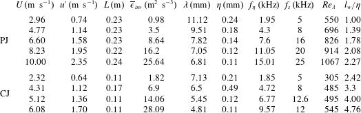
 $Re_{\unicode[STIX]{x1D706}}$ can be relatively large (table 2) when compared to the other flows (table 1). (ii) There is no shear on the jet axis and the intermittency factor associated with the turbulent/non-turbulent interface is very nearly 1 (see Bilger, Antonia & Sreenivasan Reference Bilger, Antonia and Sreenivasan1976). (iii) Local isotropy, which is a key ingredient of Kolmogorov’s similarity hypotheses, is satisfied closely (see Tang et al. (Reference Tang, Antonia, Djenidi, Abe, Zhou, Danaila and Zhou2015a,Reference Tang, Antonia, Djenidi and Zhoub), Antonia et al. (Reference Antonia, Tang, Djenidi and Danaila2015) and Tang et al. (Reference Tang, Antonia, Djenidi, Danaila and Zhou2018)). (iv) The flow along the axis of the circular jet is exactly self-preserving. As a result,
 $Re_{\unicode[STIX]{x1D706}}$ is constant with respect to
 $x$ (Djenidi et al. Reference Djenidi, Antonia, Lefeuvre and Lemay2016). (v) In this flow, the Reynolds number effect on the small-scale quantities such as the skewness and flatness factors of
 $\unicode[STIX]{x2202}u/\unicode[STIX]{x2202}x$ disappears more rapidly as the Reynolds number increases than in other flows, including grid turbulence and forced DNS box turbulence (Tang et al. Reference Tang, Antonia, Djenidi, Danaila and Zhou2018). Since all of the experiments reported here have already been published, the reader can find detailed descriptions of the experimental conditions and measurement techniques in each flow in the original papers; the experimental uncertainty has also been discussed in those papers. For example, the major ‘systematic’ error sources when measuring the flatness factor of
 $\unicode[STIX]{x2202}u/\unicode[STIX]{x2202}x$, defined by
 $$\begin{eqnarray}F=\frac{\overline{(\unicode[STIX]{x2202}u/\unicode[STIX]{x2202}x)^{4}}}{\overline{(\unicode[STIX]{x2202}u/\unicode[STIX]{x2202}x)^{2}}^{2}},\end{eqnarray}$$
which the smallest-scale quantity of  $\unicode[STIX]{x1D6F9}(r)$ since
 $\unicode[STIX]{x1D6F9}(r)\rightarrow F$ in the limit
 $r\rightarrow 0$, have been discussed in detail in Tang et al. (Reference Tang, Antonia, Djenidi, Danaila and Zhou2018) where it was found that their effect on
 $F$ is negligible, which gives us confidence that
 $\unicode[STIX]{x1D6F9}(r)$ has been measured with sufficient accuracy. In particular, the Kolmogorov-normalized one-dimensional velocity spectra collapse quite well in the dissipative range for all the present data and the high resolution DNS spectrum on the centreline of a fully developed channel flow (see figure 1a), implying that the dissipation range of the present data is fully resolved. The main flow parameters in each experiment are shown in tables 1 and 2 where
 $f_{s}$ is the sampling frequency;
 $f_{\unicode[STIX]{x1D702}}=U/2\unicode[STIX]{x03C0}\unicode[STIX]{x1D702}$ is the Kolmogorov frequency;
 $l_{w}$ is the hot-wire length. Except for the plane jet and channel flow, where a smaller wire diameter (
 $d_{w}=1.27~\unicode[STIX]{x03BC}\text{m}$) was used to avoid spectral attenuation due to the wire length effect,
 $d_{w}=2.5~\unicode[STIX]{x03BC}\text{m}$ was used for all other hot-wire measurements. In the present paper, we use a surrogate
 $$\begin{eqnarray}\unicode[STIX]{x1D716}=15\unicode[STIX]{x1D708}(\unicode[STIX]{x2202}u/\unicode[STIX]{x2202}x)^{2}=-15\frac{\unicode[STIX]{x1D708}}{U}(\unicode[STIX]{x2202}u/\unicode[STIX]{x2202}t)^{2},\end{eqnarray}$$
Main flow parameters in various flows. GT denotes grid turbulence, CC circular cylinder wake, SS screen strip wake and CF fully developed turbulent channel flow.

as has been done in the past (e.g. Nelkin Reference Nelkin1981; Antonia et al. Reference Antonia, Satyaprakash and Hussain1982; Sreenivasan & Kailasnath Reference Sreenivasan and Kailasnath1993; Praskovsky & Oncley Reference Praskovsky and Oncley1994; Cleve et al. Reference Cleve, Greiner and Sreenivasan2003, Reference Cleve, Greiner, Pearson and Sreenivasan2004), to examine the behaviour of  $\unicode[STIX]{x1D6F9}$. It is worth recalling that, in both the laboratory (Mydlarski & Warhaft Reference Mydlarski and Warhaft1996; Shafi, Zhu & Antonia Reference Shafi, Zhu and Antonia1997) and the atmospheric boundary layer (Cleve et al. Reference Cleve, Greiner and Sreenivasan2003), different surrogates such as
 $(\unicode[STIX]{x2202}u/\unicode[STIX]{x2202}x)^{2}$,
 $(\unicode[STIX]{x2202}v/\unicode[STIX]{x2202}x)^{2}$ and
 $(\unicode[STIX]{x2202}u/\unicode[STIX]{x2202}y)^{2}$ have yielded the same value for
 $\unicode[STIX]{x1D707}$. Using DNS data for forced box turbulence, Hosokawa, Oide & Yamamoto (Reference Hosokawa, Oide and Yamamoto1996) reported differences between the scaling exponents of the true
 $\unicode[STIX]{x1D716}$ and its surrogate. However, Stolovitzky, Meneveau & Sreenivasan (Reference Stolovitzky, Meneveau and Sreenivasan1998) noted that, provided an adequate averaging time is used, the difference reported by Hosokawa et al. (Reference Hosokawa, Oide and Yamamoto1996) could in fact disappear. The previous observations imply that the power-law behaviour of
 $\unicode[STIX]{x1D6F9}$ does not depend on the use of Taylor’s hypothesis and should not depend significantly on the choice of the surrogate. Nonetheless, we cannot completely rule out the possibility that the behaviour of
 $\unicode[STIX]{x1D6F9}$, based on the true
 $\unicode[STIX]{x1D716}$, may differ from that based on a surrogate quantity; such a difference does not, in any case, invalidate the question of whether a small-scale quantity such as
 $(\unicode[STIX]{x2202}u/\unicode[STIX]{x2202}x)^{2}$ scales on
 $\overline{\unicode[STIX]{x1D716}}$ and
 $\unicode[STIX]{x1D708}$ or if, in fact, it scales on
 $L$.
Main flow parameters along the axes of a plane jet (PJ) and circular jet (CJ). Note that all the PJ data were measured at a location  $36D$ downstream from the exit, where
 $D$ is the height of the two-dimensional nozzle. Note also that the CJ data at
 $Re_{\unicode[STIX]{x1D706}}=485$ were measured at
 $x/D=60$, where
 $D$ is the diameter of the jet nozzle, whereas the other CJ data were measured at
 $x/D=40$.

2.1 Estimations of  $\overline{\unicode[STIX]{x1D716}}$ and $L$


As noted in the introduction, the main objective of this paper is to decide between two completely different types of scaling, i.e. (1.3) versus (1.4). Therefore, it is important to check the accuracy of  $\overline{\unicode[STIX]{x1D716}}$ and
 $L$ before discussing the results. Although we use the isotropic value of
 $\overline{\unicode[STIX]{x1D716}}$, obtained by averaging (2.2), we are confident that
 $\overline{\unicode[STIX]{x1D716}}$ closely approximates
 $\overline{\unicode[STIX]{x1D716}_{t}}$ (
 $\overline{\unicode[STIX]{x1D716}_{t}}$ is the actual dissipation rate), if we restrict our attention to the flows described above, i.e. grid turbulence, along the axes of wakes and jets, and along the centreline of a fully developed channel flow. For example, for grid turbulence at low
 $Re_{\unicode[STIX]{x1D706}}\approx 50$, the 3-component vorticity measurements of Antonia, Zhou & Zhu (Reference Antonia, Zhou and Zhu1998) indicated that
 $\overline{\unicode[STIX]{x1D716}}$ represents a good approximation (
 $\pm 5\,\%$) to the value inferred from the decay rate of
 $\overline{q^{2}}$, i.e.
 $$\begin{eqnarray}\bar{\unicode[STIX]{x1D716}}\approx -\frac{1}{2}U\frac{\unicode[STIX]{x2202}\overline{q^{2}}}{\unicode[STIX]{x2202}x}=\overline{\unicode[STIX]{x1D716}_{t}},\end{eqnarray}$$
or from the directly measured mean enstrophy ( $\unicode[STIX]{x1D708}\overline{\unicode[STIX]{x1D714}_{i}\unicode[STIX]{x1D714}_{i}}$). This is further supported by the grid turbulence DNS data of Djenidi & Antonia (Reference Djenidi and Antonia2014) which show that
 $\overline{\unicode[STIX]{x1D716}}\approx \overline{\unicode[STIX]{x1D716}_{t}}\approx \unicode[STIX]{x1D708}\overline{\unicode[STIX]{x1D714}_{i}\unicode[STIX]{x1D714}_{i}}$. Similarly, along the axis of the round jet, the measurements of Djenidi et al. (Reference Djenidi, Antonia, Lefeuvre and Lemay2016) indicated that
 $\bar{\unicode[STIX]{x1D716}}$ is in good agreement with the value inferred from the transport equation of
 $\overline{q^{2}}$. Further, Djenidi & Antonia (Reference Djenidi and Antonia2012) proposed a spectral chart method for estimating
 $\overline{\unicode[STIX]{x1D716}_{t}}$. The basis for this method is the expected collapse of the energy spectra in the dissipation range, when normalized by
 $\bar{\unicode[STIX]{x1D716}}$ and
 $\unicode[STIX]{x1D708}$. A plausible analytical underpinning of this collapse was provided by Antonia et al. (Reference Antonia, Djenidi and Danaila2014). Tang et al. (Reference Tang, Antonia, Djenidi and Zhou2015b) tested this method in some detail in the far wake of a circular cylinder; they showed that the mean energy dissipation estimated by the spectral chart method is in good agreement (
 $\pm 5\,\%$) with the measurement of
 $\overline{\unicode[STIX]{x1D716}_{t}}$ (Browne, Antonia & Shah Reference Browne, Antonia and Shah1987) and the estimation based on the transport equation of
 $\overline{q^{2}}$. Figure 1(a) shows the Kolmogorov-normalized spectra of
 $u$ for all flows considered; the normalization is based on
 $\bar{\unicode[STIX]{x1D716}}$ and
 $\unicode[STIX]{x1D708}$. For reference, the velocity spectrum on the centreline of a fully developed channel flow, normalized by
 $\overline{\unicode[STIX]{x1D716}_{t}}$ and
 $\unicode[STIX]{x1D708}$, is shown (Abe, Antonia & Kawamura Reference Abe, Antonia and Kawamura2009). There is good collapse over most of the dissipative range, suggesting that the difference between
 $\bar{\unicode[STIX]{x1D716}}$ and
 $\overline{\unicode[STIX]{x1D716}_{t}}$, the true value of the mean energy dissipation, cannot be significant.
(a) One-dimensional longitudinal velocity spectra, normalized by  $\overline{\unicode[STIX]{x1D716}}$ and
 $\unicode[STIX]{x1D708}$. (a) Red curves: grid turbulence; (b) black curves: along the centreline of a fully developed channel flow; (c) blue and pink curves correspond to the flows along the axes of wakes generated with two different initial conditions: a solid circular cylinder and a screen strip, respectively; (d) yellow and green curves correspond to the flows along the axes of circular and plane jets, respectively. For reference, the DNS spectrum on the centreline of a fully developed channel flow (black dashed curve), normalized by
 $\overline{\unicode[STIX]{x1D716}_{t}}$ and
 $\unicode[STIX]{x1D708}$, is shown (Abe et al. Reference Abe, Antonia and Kawamura2009). (b)
 $C_{\unicode[STIX]{x1D716}}=\overline{\unicode[STIX]{x1D716}}L/u^{\prime 3}$ for the plane (▪) and circular (▴, Mi, Xu & Zhou (Reference Mi, Xu and Zhou2013); ●, present data; ♦, Djenidi et al. (Reference Djenidi, Lefeuvre, Kamruzzaman and Antonia2017)) jets respectively. Also included are the data in stationary forced periodic box turbulence (▾) (Ishihara, Gotoh & Kaneda Reference Ishihara, Gotoh and Kaneda2009) without identifying the sources.

Finally, instead of discussing the accuracy of  $L$, we briefly discuss the non-dimensional dissipation rate parameter, which is closely related to
 $L$, i.e.
 $$\begin{eqnarray}C_{\unicode[STIX]{x1D716}}\equiv \overline{\unicode[STIX]{x1D716}}L/u^{\prime 3},\end{eqnarray}$$
which was first introduced by Taylor (Reference Taylor1935) via a dimensional argument;  $L$ is the integral length scale defined by
 $L=U\int _{0}^{\unicode[STIX]{x1D70F}_{0}}\unicode[STIX]{x1D70C}_{uu}(\unicode[STIX]{x1D70F})\,\text{d}\unicode[STIX]{x1D70F}$,
 $\unicode[STIX]{x1D70C}_{uu}(\unicode[STIX]{x1D70F})$ is the longitudinal autocorrelation function and
 $\unicode[STIX]{x1D70F}_{0}$ is the time corresponding to the first zero crossing of
 $\unicode[STIX]{x1D70C}_{uu}(\unicode[STIX]{x1D70F})$. It seems that
 $C_{\unicode[STIX]{x1D716}}=\text{const.}$, independently of
 $Re_{\unicode[STIX]{x1D706}}$, can be achieved at a value of
 $Re_{\unicode[STIX]{x1D706}}$ of approximately 100 (e.g. Sreenivasan Reference Sreenivasan1984; Burattini, Lavoie & Antonia Reference Burattini, Lavoie and Antonia2005; Goto & Vassilicos Reference Goto and Vassilicos2009; Ishihara et al. Reference Ishihara, Gotoh and Kaneda2009; McComb et al. Reference McComb, Berera, Yoffe and Linkmann2015; Vassilicos Reference Vassilicos2015; Linkmann Reference Linkmann2018) in many flows, but the magnitude of this constant may differ between flows. Figure 1(b) shows the plane and circular jet data for
 $C_{\unicode[STIX]{x1D716}}$. For reference, we have also included, without identifying the sources, the data of Ishihara et al. (Reference Ishihara, Gotoh and Kaneda2009) for stationary forced periodic box turbulence. For the present plane jet data,
 $C_{\unicode[STIX]{x1D716}}$ is approximately constant (approximately 0.50) up to
 $Re_{\unicode[STIX]{x1D706}}\approx 1100$ and in reasonable agreement with Ishihara et al.’s data (Ishihara et al. Reference Ishihara, Gotoh and Kaneda2009) over a comparable range of
 $Re_{\unicode[STIX]{x1D706}}$. The magnitude of
 $C_{\unicode[STIX]{x1D716}}$ is slightly larger on the axis of the circular jet; the present values are in reasonable agreement with those obtained in other investigations. Further, on the axes of the plane and circular jets, the magnitude of
 $L$ is practically independent of
 $Re_{\unicode[STIX]{x1D706}}$ at a fixed value of
 $x/D$, see table 2. This reflects the fact the Reynolds number is of little importance as far as the large scales are concerned. It also means that
 $\overline{\unicode[STIX]{x1D716}}$ should vary with
 $u^{\prime 3}$, which is confirmed by the data in table 2 since
 $C_{\unicode[STIX]{x1D716}}$ is approximately constant with respect to
 $Re_{\unicode[STIX]{x1D706}}$ (figure 1b). It would seem that, in the context of deciding between (1.3) and (1.4), the accuracy of
 $L$ is much less important than the accuracy of
 $\overline{\unicode[STIX]{x1D716}}$.
3 Results
3.1 Value of $\unicode[STIX]{x1D6F9}(r^{\ast })$ at small to moderate $Re_{\unicode[STIX]{x1D706}}$


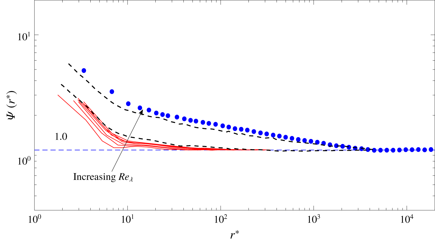
Autocorrelation function  $\unicode[STIX]{x1D6F9}(r^{\ast })$ in grid turbulence. Red curves: present data (
 $Re_{\unicode[STIX]{x1D706}}=27{-}100$). Dashed black curves: Mydlarski & Warhaft (Reference Mydlarski and Warhaft1996) (
 $Re_{\unicode[STIX]{x1D706}}=100$ and 377). The arrow is in the direction of increasing
 $Re_{\unicode[STIX]{x1D706}}$. The horizontal line indicates the value of 1. As reference, also shown are the circular jet data at
 $Re_{\unicode[STIX]{x1D706}}=485$ (●), which will be discussed in the context of figure 5.

Autocorrelation function  $\unicode[STIX]{x1D6F9}(r^{\ast })$ along the centreline of a fully developed channel flow for
 $Re_{\unicode[STIX]{x1D706}}=33{-}120$ (black curves). Other symbols and lines are as in figure 2.

Autocorrelation function  $\unicode[STIX]{x1D6F9}(r^{\ast })$ along the axes of wakes generated with two different initial conditions: a solid circular cylinder (blue curves,
 $Re_{\unicode[STIX]{x1D706}}=161{-}274$) and a screen strip (pink curves,
 $Re_{\unicode[STIX]{x1D706}}=123{-}222$). Other symbols and lines are as in figure 2.

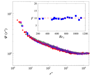
Autocorrelation function  $\unicode[STIX]{x1D6F9}(r^{\ast })$ in plane and circular jets; plane jet (
 $Re_{\unicode[STIX]{x1D706}}=550$ (▿), 696 (
 $\times$), 826 (▵), 914 (○) and 1067 (▫)); circular jet (305 (▪), 485 (●), 495 (▾) and 545 (▴)). Also shown are the circular jet data at
 $Re_{\unicode[STIX]{x1D706}}=966$ (
 $\ast$, Antonia, Phan-Thien & Satyaprakash (Reference Antonia, Phan-Thien and Satyaprakash1981)). The distribution for
 $-\overline{(\unicode[STIX]{x1D6FF}u^{\ast })^{3}}/r^{\ast }$ on the axis of the plane jet at
 $Re_{\unicode[STIX]{x1D706}}=1067$ is also shown for comparison of the scaling range. Blue dashed line: 0.8. The arrowed horizontal line indicates the extent of the scaling range, based on an arbitrary (5 %) departure from the maximum value of
 $-\overline{(\unicode[STIX]{x1D6FF}u^{\ast })^{3}}/r^{\ast }$. The vertical arrow indicates the magnitude of the Taylor microscale (
 $\unicode[STIX]{x1D706}/\unicode[STIX]{x1D702}$) at
 $Re_{\unicode[STIX]{x1D706}}=1067$. The inset shows the dependence of
 $F$ on
 $Re_{\unicode[STIX]{x1D706}}$ in circular and plane jets; they are reproduced from figure 1 of Tang et al. (Reference Tang, Antonia, Djenidi and Zhou2019) without identifying the data sources. The red dashed line indicates a value of 10.

In the limit  $r\rightarrow 0$,
 $\unicode[STIX]{x1D6F9}(r)$ reduces to
 $F$. Tang et al. (Reference Tang, Antonia, Djenidi, Danaila and Zhou2018) showed that the magnitude of
 $F$ depends on
 $Re_{\unicode[STIX]{x1D706}}$ as well as the flow when
 $Re_{\unicode[STIX]{x1D706}}$ is small or moderate. It is thus most likely that
 $\unicode[STIX]{x1D6F9}(r^{\ast })$ should also depend on
 $Re_{\unicode[STIX]{x1D706}}$ and the type of flow at small to moderate
 $Re_{\unicode[STIX]{x1D706}}$. To verify this, we consider data for
 $\unicode[STIX]{x1D6F9}(r^{\ast })$ in a wide range of flows, e.g. grid turbulence, along the centreline of a fully developed channel flow and along the axes of wakes, which were generated by two different initial conditions: a solid circular cylinder and a screen strip. Separate plots are used (figures 2–4), with the same scales for the vertical and horizontal axes. The circular jet data at
 $Re_{\unicode[STIX]{x1D706}}=485$ are shown as reference on each plot since they are representative of all the circular jet data in the range
 $305<Re_{\unicode[STIX]{x1D706}}<966$; this will be discussed in the context of figure 5. As expected,
 $\unicode[STIX]{x1D6F9}(r^{\ast })$ approaches a constant (
 ${\approx}1$, see figures 2–4) in the limit of
 $r\rightarrow \infty$. Further, the distributions of
 $\unicode[STIX]{x1D6F9}(r^{\ast })$ in each flow show an unmistakable systematic increase as
 $Re_{\unicode[STIX]{x1D706}}$ increases. For the grid turbulence data at
 $Re_{\unicode[STIX]{x1D706}}\approx 100$ (figure 2), there is adequate agreement between the present data and those of Mydlarski & Warhaft (Reference Mydlarski and Warhaft1996). At
 $Re_{\unicode[STIX]{x1D706}}\approx 377$, the magnitude of
 $\unicode[STIX]{x1D6F9}(r^{\ast })$ is slightly smaller than in the circular jet at
 $Re_{\unicode[STIX]{x1D706}}\approx 485$. This implies that the FRN effect on
 $\unicode[STIX]{x1D6F9}(r^{\ast })$ disappears gradually as
 $Re_{\unicode[STIX]{x1D706}}$ increases. This is consistent with the behaviour of
 $F$, which increases with increasing
 $Re_{\unicode[STIX]{x1D706}}$ and is very nearly constant (
 ${\approx}11.2$) for
 $Re_{\unicode[STIX]{x1D706}}>600$ (Tang et al. Reference Tang, Antonia, Djenidi, Danaila and Zhou2018). Along the centreline of the channel flow,
 $\unicode[STIX]{x1D6F9}(r^{\ast })$ is significantly smaller than the reference distribution due to the relatively small
 $Re_{\unicode[STIX]{x1D706}}$ (
 $=33{-}120$). Figure 4 shows the distributions of
 $\unicode[STIX]{x1D6F9}(r^{\ast })$ along the axes of the two wakes (solid circular cylinder
 $Re_{\unicode[STIX]{x1D706}}=161{-}274$) and screen strip
 $Re_{\unicode[STIX]{x1D706}}=123{-}222$). The magnitude of
 $\unicode[STIX]{x1D6F9}(r^{\ast })$ is larger for the screen strip wake than for the circular cylinder wake even though
 $Re_{\unicode[STIX]{x1D706}}$ is smaller in the former case. This implies that the initial conditions can affect
 $\unicode[STIX]{x1D6F9}(r^{\ast })$ significantly. Overall, figures 2–4 show that there is a relatively strong variation with
 $Re_{\unicode[STIX]{x1D706}}$ in both the shape and magnitude of
 $\unicode[STIX]{x1D6F9}(r^{\ast })$ at low
 $Re_{\unicode[STIX]{x1D706}}$. Whilst the variation with
 $Re_{\unicode[STIX]{x1D706}}$ is systematic for a given flow, the actual magnitude of
 $\unicode[STIX]{x1D6F9}(r^{\ast })$ may not be the same at a similar
 $Re_{\unicode[STIX]{x1D706}}$ among different flows when
 $Re_{\unicode[STIX]{x1D706}}$ is small or moderate. We have shown previously (e.g. Antonia et al. Reference Antonia, Tang, Djenidi and Danaila2015), using the Kármán–Howarth equation as the starting point, that the skewness of
 $\unicode[STIX]{x2202}u/\unicode[STIX]{x2202}x$ defined by
 $$\begin{eqnarray}S=\frac{\overline{(\unicode[STIX]{x2202}u/\unicode[STIX]{x2202}x)^{3}}}{\overline{(\unicode[STIX]{x2202}u/\unicode[STIX]{x2202}x)^{2}}^{3/2}},\end{eqnarray}$$
will approach a constant value when  $Re_{\unicode[STIX]{x1D706}}$ is sufficiently large, but the way this constant is approached is flow dependent because the FRN effect may differ in different flows. It is thus most likely that
 $\unicode[STIX]{x1D6F9}$ will exhibit a similar behaviour in different flows at small to moderate
 $Re_{\unicode[STIX]{x1D706}}$. Note that the maximum
 $Re_{\unicode[STIX]{x1D706}}$ in figures 2–4 is only 377.
3.2 Values of $\unicode[STIX]{x1D6F9}(r^{\ast })$ and $\unicode[STIX]{x1D6F9}(r/L)$ at larger $Re_{\unicode[STIX]{x1D706}}$


For the circular jet ( $Re_{\unicode[STIX]{x1D706}}=305{-}966$) and plane jet data (
 $Re_{\unicode[STIX]{x1D706}}=550{-}1067$) in figure 5, the distributions for
 $\unicode[STIX]{x1D6F9}(r^{\ast })$ collapse onto a single distribution, implying the disappearance of the FRN effect on
 $\unicode[STIX]{x1D6F9}(r^{\ast })$, at least for circular and plane jets. The main message of figures 2–4 is that the magnitude of
 $\unicode[STIX]{x1D6F9}(r^{\ast })$ differs from flow to flow at small to moderate
 $Re_{\unicode[STIX]{x1D706}}$. More importantly,
 $\unicode[STIX]{x1D6F9}(r^{\ast })$ continues to increase as
 $Re_{\unicode[STIX]{x1D706}}$ increases. Figure 5 indicates that, for circular and plane jets,
 $\unicode[STIX]{x1D6F9}(r^{\ast })$ becomes independent of
 $Re_{\unicode[STIX]{x1D706}}$ beyond
 $Re_{\unicode[STIX]{x1D706}}\approx 300$. This collapse in figure 5 is consistent with Kolmogorov’s first similarity hypothesis, i.e. (1.4). However, we note that the laboratory data for
 $\unicode[STIX]{x1D6F9}(r^{\ast })$ in figures 2–5 do not exclude the possibility that the final (
 $Re_{\unicode[STIX]{x1D706}}$-independent) distribution of
 $\unicode[STIX]{x1D6F9}(r^{\ast })$ when
 $Re_{\unicode[STIX]{x1D706}}$ is sufficiently large may differ in each flow, i.e. there may not be a unique distribution of
 $\unicode[STIX]{x1D6F9}(r^{\ast })$. Evidently, it would be desirable to further investigate this by continuing to increase
 $Re_{\unicode[STIX]{x1D706}}$ in flows such as the grid turbulence, wakes and channel flows. Nevertheless, the collapse at small
 $r^{\ast }$ of
 $\unicode[STIX]{x1D6F9}(r^{\ast })$ in figure 5 is consistent with the behaviour of
 $F$ since
 $\unicode[STIX]{x1D6F9}(r^{\ast })=F$ in the limit
 $r\rightarrow 0$;
 $F$ approaches a constant, which may not be universal, as
 $Re_{\unicode[STIX]{x1D706}}$ increases (Tang et al. Reference Tang, Antonia, Djenidi, Danaila and Zhou2018).
The local slope of  $\unicode[STIX]{x1D6F9}(r^{\ast })$ (
 $=\mathit{d}\log \unicode[STIX]{x1D6F9}(r^{\ast })/\mathit{d}\log r^{\ast }$) corresponding to the plane jet data in figure 5. The arrowed horizontal line indicates the extent of the power-law range. Symbols are the same as in figure 5. The blue and red dashed lines correspond to the values of
 $-0.17$ and 0, respectively.

In figure 5, we can also observe a significant range ( $30\lesssim r^{\ast }\lesssim 400$) where
 $\unicode[STIX]{x1D6F9}(r^{\ast })$ decays according to a power law. The local slope of
 $\unicode[STIX]{x1D6F9}(r^{\ast })=\mathit{d}\log \unicode[STIX]{x1D6F9}(r^{\ast })/\mathit{d}\log r^{\ast }$ for the plane jet data as a function of
 $r^{\ast }$ is shown in figure 6 with a linear ordinate. Since
 $\unicode[STIX]{x1D6F9}(r^{\ast })$ collapses at all
 $r^{\ast }$, the corresponding local slope has a unique distribution. At large
 $r^{\ast }$, the local slope approaches zero since
 $\unicode[STIX]{x1D6F9}(r^{\ast })$ approaches the constant value of 1. Over the range
 $30\lesssim r^{\ast }\lesssim 400$, figure 6 shows that there is an unambiguous plateau corresponding to
 $=\mathit{d}\log \unicode[STIX]{x1D6F9}(r^{\ast })/\mathit{d}\log r^{\ast }\approx -0.17$. In this range,
 $\unicode[STIX]{x1D6F9}(r^{\ast })$ can be written as
 $$\begin{eqnarray}\unicode[STIX]{x1D6F9}(r^{\ast })=C_{\unicode[STIX]{x1D716}\unicode[STIX]{x1D716}}r^{\ast -\unicode[STIX]{x1D707}},\end{eqnarray}$$
where  $C_{\unicode[STIX]{x1D716}\unicode[STIX]{x1D716}}=3.6\pm 0.1$ and
 $\unicode[STIX]{x1D707}=0.17\pm 0.01$. Both
 $\unicode[STIX]{x1D707}$ and
 $C_{\unicode[STIX]{x1D716}\unicode[STIX]{x1D716}}$ are independent of
 $Re_{\unicode[STIX]{x1D706}}$ when
 $Re_{\unicode[STIX]{x1D706}}\gtrsim 300$. The extent of the power-law range observed here (
 $30\lesssim r^{\ast }\lesssim 400$) is fixed. The beginning and end points of this range are independent of
 $Re_{\unicode[STIX]{x1D706}}$. At this stage, the relationship between this range and Kolmogorov’s (Reference Kolmogorov1941a) inertial range, which can only occur at extremely large values of
 $Re_{\unicode[STIX]{x1D706}}$, is not known. It is evident, however, that the power-law range of
 $\unicode[STIX]{x1D6F9}(r^{\ast })$ overlaps the so-called scaling range. This is also shown in figure 5; it is based on an arbitrary (5 %) departure from the maximum value of
 $-\overline{(\unicode[STIX]{x1D6FF}u^{\ast })^{3}}/r^{\ast }$. The extent of the scaling range lies within the extent of the power-law range for
 $\unicode[STIX]{x1D6F9}$. We have included in figure 5 a distribution of
 $-\overline{(\unicode[STIX]{x1D6FF}u^{\ast })^{3}}/r^{\ast }$ at the largest value of
 $Re_{\unicode[STIX]{x1D706}}$ for the plane jet. The convex curvature about the maximum is symptomatic of all distributions of
 $-\overline{(\unicode[STIX]{x1D6FF}u^{\ast })^{3}}/r^{\ast }$ that have been reported in the literature (Antonia et al. Reference Antonia, Tang, Djenidi and Zhou2019). The location of the maximum is close to
 $r=\unicode[STIX]{x1D706}$ (e.g. Lundgren Reference Lundgren2003; Antonia & Burattini Reference Antonia and Burattini2006; Boschung et al. Reference Boschung, Gauding, Hennig, Denker and Pitsch2016); the value of
 $\unicode[STIX]{x1D706}^{\ast }$ is indicated by the vertical arrow in figure 5.
We recall that the two limits:  $\unicode[STIX]{x1D6F9}(r)\rightarrow F$ and
 $\unicode[STIX]{x1D6F9}(r)\rightarrow 1$ when
 $r\rightarrow 0$ and
 $r$ exceeds
 $L$, respectively, are unchanged regardless of whether we assume that
 $\unicode[STIX]{x1D6F9}(r)$ scales on K41 or K62. These limits are bounded, see for example the inset of figure 5. One therefore expects that, in the power-law range,
 $\unicode[STIX]{x1D6F9}(r)$ should also be bounded. Since
 $\overline{\unicode[STIX]{x1D716}(x+r)}\leqslant \overline{\unicode[STIX]{x1D716}(x)}$ for decaying-type turbulence (e.g.
 $\overline{\unicode[STIX]{x1D716}(x)}\sim x^{-4}$ along the axis of a circular jet in the far field or
 $\overline{\unicode[STIX]{x1D716}(x)}\sim x^{n-1}$ in grid turbulence where
 $\overline{q^{2}}=\overline{u^{2}}+\overline{v^{2}}+\overline{w^{2}}\sim x^{n}$), application of the Cauchy–Schwarz theorem to
 $\unicode[STIX]{x1D6F9}(r)$ yields
 $$\begin{eqnarray}\unicode[STIX]{x1D6F9}(r)=\frac{\overline{\unicode[STIX]{x1D716}(x)\unicode[STIX]{x1D716}(x+r)}}{\overline{\unicode[STIX]{x1D716}(x)}^{2}}\leqslant \frac{\overline{\unicode[STIX]{x1D716}^{2}(x)}^{1/2}\overline{\unicode[STIX]{x1D716}^{2}(x+r)}^{1/2}}{\overline{\unicode[STIX]{x1D716}(x)}^{2}}\leqslant \frac{\overline{\unicode[STIX]{x1D716}^{2}(x)}^{1/2}}{\overline{\unicode[STIX]{x1D716}(x)}}\frac{\overline{\unicode[STIX]{x1D716}^{2}(x+r)}^{1/2}}{\overline{\unicode[STIX]{x1D716}(x+r)}}.\end{eqnarray}$$
Replacing  $\unicode[STIX]{x1D716}$ by
 $15\unicode[STIX]{x1D708}(\unicode[STIX]{x2202}u/\unicode[STIX]{x2202}x)^{2}$, equation (3.3) yields
 $$\begin{eqnarray}\unicode[STIX]{x1D6F9}(r)\leqslant \frac{\overline{\left({\displaystyle \frac{\unicode[STIX]{x2202}u}{\unicode[STIX]{x2202}x}}\right)^{4}(x)}^{1/2}}{\overline{\left({\displaystyle \frac{\unicode[STIX]{x2202}u}{\unicode[STIX]{x2202}x}}\right)^{2}(x)}}\frac{\overline{\left({\displaystyle \frac{\unicode[STIX]{x2202}u}{\unicode[STIX]{x2202}x}}\right)^{4}(x+r)}^{1/2}}{\overline{\left({\displaystyle \frac{\unicode[STIX]{x2202}u}{\unicode[STIX]{x2202}x}}\right)^{2}(x+r)}}=F^{1/2}(x)F^{1/2}(x+r).\end{eqnarray}$$
Since  $F$ is bounded,
 $\unicode[STIX]{x1D6F9}(r)$ should also be bounded regardless of whether
 $\unicode[STIX]{x1D6F9}(r)$ scales on K41 or K62 in the power-law range. However, the K62 framework assumes
 $\unicode[STIX]{x1D6F9}(r)=D(r/L)^{-\unicode[STIX]{x1D707}}$, equation (1.3). For
 $r=\unicode[STIX]{x1D706}$, the location where
 $-\overline{(\unicode[STIX]{x1D6FF}u^{\ast })^{3}}/r^{\ast }$ is close its maximum value,
 $\unicode[STIX]{x1D6F9}(\unicode[STIX]{x1D706})$ is given by
 $D(C_{\unicode[STIX]{x1D716}}Re_{\unicode[STIX]{x1D706}}/15)^{\unicode[STIX]{x1D707}}$ for locally isotropic turbulence. This implies that the magnitude of
 $\unicode[STIX]{x1D6F9}(r)$ in the power-law range should increase indefinitely with
 $Re_{\unicode[STIX]{x1D706}}$, which violates (3.4). On the other hand, if we set
 $r=\unicode[STIX]{x1D706}$ in (3.2), we find that
 $\unicode[STIX]{x1D6F9}(\unicode[STIX]{x1D706}^{\ast })=C_{\unicode[STIX]{x1D716}\unicode[STIX]{x1D716}}\unicode[STIX]{x1D706}^{-\ast \unicode[STIX]{x1D707}}$. For locally isotropic turbulence,
 $\unicode[STIX]{x1D706}^{\ast }=15^{1/4}Re_{\unicode[STIX]{x1D706}}^{1/2}$ so that
 $\unicode[STIX]{x1D6F9}(\unicode[STIX]{x1D706}^{\ast })\sim \unicode[STIX]{x1D706}^{-\ast \unicode[STIX]{x1D707}/2}$ will approach zero as
 $Re_{\unicode[STIX]{x1D706}}$ increases; this trend does not violate (3.4). The above observations, together with the collapse of
 $\unicode[STIX]{x1D6F9}(r^{\ast })$ in figure 5, strongly imply that similarity based on the external length scale
 $L$ is untenable. Note here that the appearance of
 $L$ in (1.2) also leads to the unphysical scenario that, when
 $r=\unicode[STIX]{x1D706}$,
 $\overline{(\unicode[STIX]{x1D6FF}u)^{2}}$ will grow indefinitely as
 $Re_{\unicode[STIX]{x1D706}}$ increases.
The autocorrelation function  $\unicode[STIX]{x1D6F9}(r/L)$ in plane and circular jets. Symbols are the same as in figure 5. Also shown are the plane and circular jet data for
 $Re_{\unicode[STIX]{x1D706}}\simeq 380{-}720$ (●, Antonia et al. (Reference Antonia, Satyaprakash and Hussain1982)) without identifying the sources. The inset shows a corresponding enlargement at relatively small
 $r/L$. For clarity, only the present plane jet data are shown in this inset.

Figure 7 shows the distributions of  $\unicode[STIX]{x1D6F9}(r/L)$ for the same plane and circular jet data. Also shown are the plane and circular jet data of Antonia et al. (Reference Antonia, Satyaprakash and Hussain1982) for
 $Re_{\unicode[STIX]{x1D706}}\simeq 380{-}720$ without identifying the sources. It can be seen that there is no collapse for
 $\unicode[STIX]{x1D6F9}(r/L)$ in either the dissipative or power-law range. Instead, the variation of
 $\unicode[STIX]{x1D6F9}(r/L)$ with
 $Re_{\unicode[STIX]{x1D706}}$ is systematic (see the inset of figure 7), implying that the self-similarity of
 $\unicode[STIX]{x1D6F9}(r/L)$ as has been proposed by several authors (Yaglom Reference Yaglom1966; Gurvich & Yaglom Reference Gurvich and Yaglom1967; Monin & Yaglom Reference Monin and Yaglom1975; Nelkin Reference Nelkin2000) is not tenable. In contrast, there is a relatively good collapse for
 $\unicode[STIX]{x1D6F9}(r^{\ast })$ at large
 $Re_{\unicode[STIX]{x1D706}}$ over nearly the complete range of
 $r^{\ast }$. Note that Antonia et al.’s (Reference Antonia, Satyaprakash and Hussain1982) estimate of
 $\unicode[STIX]{x1D707}=0.2\pm 0.02$ is in reasonable agreement with the present value (
 $0.17\pm 0.01$).
An indirect estimation of  $\unicode[STIX]{x1D707}$ has been used relatively frequently in the literature (e.g. Anselmet et al. Reference Anselmet, Gagne, Hopfinger and Antonia1984; Sreenivasan & Antonia Reference Sreenivasan and Antonia1997), based on associating the sixth-order velocity structure function
 $\overline{(\unicode[STIX]{x1D6FF}u)^{6}}$ with
 $\overline{\unicode[STIX]{x1D716}(x)\unicode[STIX]{x1D716}(x+r)}$. This association was proposed by Frisch, Sulem & Nelkin (Reference Frisch, Sulem and Nelkin1978), i.e.
 $$\begin{eqnarray}\overline{(\unicode[STIX]{x1D6FF}u)^{6}}/r^{2}\sim \overline{\unicode[STIX]{x1D716}(x)\unicode[STIX]{x1D716}(x+r)}.\end{eqnarray}$$
Figure 8(a) shows the compensated structure functions  $\overline{(\unicode[STIX]{x1D6FF}u^{\ast })^{6}}r^{\ast -2}$ for the plane jet data at
 $Re_{\unicode[STIX]{x1D706}}=550$, 696, 826, 914 and 1067, respectively. For comparison, we show also the distribution of
 $\unicode[STIX]{x1D6F9}(r^{\ast })$ at the biggest
 $Re_{\unicode[STIX]{x1D706}}(=1067)$ from figure 5; it is arbitrarily shifted to facilitate the comparison (the shift does not affect
 $\unicode[STIX]{x1D707}$). The corresponding local slopes are shown in figure 8(b). Two comments can be made with regard to figure 8. (a) For all the distributions, the power-law range of
 $\unicode[STIX]{x1D6F9}(r^{\ast })$ (
 $30\lesssim r^{\ast }\lesssim 400$) is much more convincing than that of
 $\overline{(\unicode[STIX]{x1D6FF}u^{\ast })^{6}}r^{\ast -2}$; this is more emphatically observed in figure 8(b), and reflects the significant difference in behaviour between
 $\overline{(\unicode[STIX]{x1D6FF}u^{\ast })^{6}}r^{\ast -2}$ and
 $\unicode[STIX]{x1D6F9}(r^{\ast })$. (b) Arguably, the behaviour of
 $\unicode[STIX]{x1D6F9}(r^{\ast })$ is similar to that of
 $\overline{(\unicode[STIX]{x1D6FF}u^{\ast })^{6}}r^{\ast -2}$ only at
 $Re_{\unicode[STIX]{x1D706}}=914$. The former is independent of
 $Re_{\unicode[STIX]{x1D706}}$ for
 $Re_{\unicode[STIX]{x1D706}}\gtrsim 300$ (see figure 5), whereas the latter varies systematically (both in magnitude and local slope) with
 $Re_{\unicode[STIX]{x1D706}}$ up to
 $Re_{\unicode[STIX]{x1D706}}\simeq 1100$.
The previous comments imply that the behaviour of  $\unicode[STIX]{x1D6F9}(r^{\ast })$ is consistent with K41 beyond certain values of
 $Re_{\unicode[STIX]{x1D706}}$ at least in plane and circular jets, but the magnitude of
 $\overline{(\unicode[STIX]{x1D6FF}u^{\ast })^{6}}$ continues to evolve with
 $Re_{\unicode[STIX]{x1D706}}$. Both
 $\unicode[STIX]{x1D6F9}(r^{\ast })$ and
 $\overline{(\unicode[STIX]{x1D6FF}u^{\ast })^{6}}$ can differ from flow to flow and for a given flow they may depend on the initial conditions.
(a) Values of  $\overline{(\unicode[STIX]{x1D6FF}u^{\ast })^{6}}r^{\ast -2}$ (
 $Re_{\unicode[STIX]{x1D706}}=550$, 696, 826, 914 and 1067 respectively; symbols are the same as in figure 5) and
 $\unicode[STIX]{x1D6F9}(r^{\ast })$ (
 $Re_{\unicode[STIX]{x1D706}}=1067$, ●) in a plane jet. Note that
 $\unicode[STIX]{x1D6F9}(r^{\ast })$ is shown after multiplying by 270. (b) The local slopes,
 $LS_{6}(r^{\ast })=\mathit{d}\log \overline{(\unicode[STIX]{x1D6FF}u^{\ast })^{6}}/\mathit{d}\log r^{\ast }$, corresponding to the plane jet data in (a). For clarity, distributions for only two values of
 $Re_{\unicode[STIX]{x1D706}}$ (
 $=550$ and 1067) are shown but we emphasize that the variation of
 $LS_{6}(r^{\ast })$ with
 $Re_{\unicode[STIX]{x1D706}}$ is systematic. Also shown is the local slope of
 $\unicode[STIX]{x1D6F9}(r^{\ast })$ plus 2, i.e.
 $\mathit{d}\log \unicode[STIX]{x1D6F9}(r^{\ast })/\mathit{d}\log r^{\ast }+2$, for comparison. Symbols are the same as in (a). The two tagged points represent typical values of
 $LS_{6}(r^{\ast })$ in the scaling range for
 $\overline{(\unicode[STIX]{x1D6FF}u^{\ast })^{6}}$.

3.3 Other small-scale statistics
In § 3.2, we examined the scaling behaviour of the autocorrelation of  $(\unicode[STIX]{x2202}u/\unicode[STIX]{x2202}x)^{2}$. It is also of interest to examine the scaling of quantities such as
 $(\unicode[STIX]{x2202}u/\unicode[STIX]{x2202}x)^{2}-\overline{(\unicode[STIX]{x2202}u/\unicode[STIX]{x2202}x)^{2}}$ which we loosely identify with
 $\unicode[STIX]{x1D716}^{\prime }$ (
 $=\unicode[STIX]{x1D716}-\overline{\unicode[STIX]{x1D716}}$). Distributions of the correlation
 $$\begin{eqnarray}\unicode[STIX]{x1D6F9}^{\prime }(r)=\frac{\overline{\unicode[STIX]{x1D716}^{\prime }(x)\unicode[STIX]{x1D716}^{\prime }(x+r)}}{\overline{\unicode[STIX]{x1D716}}^{2}},\end{eqnarray}$$
and the corresponding spectrum  $\unicode[STIX]{x1D711}_{\unicode[STIX]{x1D716}\prime }(k_{1}^{\ast })$ are shown in figure 9 for the plane jet data. Both
 $\unicode[STIX]{x1D6F9}^{\prime }(r^{\ast })$ and
 $\unicode[STIX]{x1D711}_{\unicode[STIX]{x1D716}\prime }(k_{1}^{\ast })$ collapse convincingly with
 $\unicode[STIX]{x1D708}$ and
 $\overline{\unicode[STIX]{x1D716}}$ for nearly the complete range of
 $r^{\ast }$ and
 $k_{1}^{\ast }$. This rules out the likelihood of scaling on external scales.
(a) Autocorrelation function  $\unicode[STIX]{x1D6F9}^{\prime }(r^{\ast })$ on the axis of the plane jet. Symbols are as in figure 5. (b) Spectrum of
 $\unicode[STIX]{x1D716}^{\prime }$;
 $Re_{\unicode[STIX]{x1D706}}=550$ (black), 696 (blue), 826 (red), 914 (pink) and 1067 (green) respectively. For clarity, only the plane jet data are shown.

Autocorrelation functions  $\unicode[STIX]{x1D6F9}_{v}(r^{\ast })$ on the axes of plane and circular jets. Symbols are as in figure 5. The black line indicates the power-law distribution
 ${\sim}r^{-0.17}$. The insets (a) and (b) show the distributions of
 $\overline{\unicode[STIX]{x1D716}}_{v}/\overline{\unicode[STIX]{x1D716}}$ and
 $F_{\unicode[STIX]{x2202}v/\unicode[STIX]{x2202}x}$ respectively in plane (▪) and circular (●) jets. The dashed blue line in inset (a) indicates the isotropic ratio of 1 whereas the dashed red lines indicate a departure of 10 % from the isotropic value of one. The red dashed line in inset (b) indicates the mean value of
 $F_{\unicode[STIX]{x2202}v/\unicode[STIX]{x2202}x}$.

We conclude this short subsection by examining the scaling of the autocorrelation function of  $(\unicode[STIX]{x2202}v/\unicode[STIX]{x2202}x)^{2}$. Defining
 $\unicode[STIX]{x1D716}_{v}=7.5\unicode[STIX]{x1D708}(\unicode[STIX]{x2202}v/\unicode[STIX]{x2202}x)^{2}$, the function
 $$\begin{eqnarray}\unicode[STIX]{x1D6F9}_{v}(r)=\overline{\unicode[STIX]{x1D716}_{v}(x)\unicode[STIX]{x1D716}_{v}(x+r)}/\overline{\unicode[STIX]{x1D716}_{v}}^{2}\end{eqnarray}$$
is plotted in figure 10 for circular and plane jet data. Some remarks are warranted before discussing the behaviour of  $\unicode[STIX]{x1D6F9}_{v}(r^{\ast })$. First, as shown in inset (a) of figure 10, the departure from local isotropy in the context of
 $\overline{\unicode[STIX]{x1D716}}_{v}\approx \overline{\unicode[STIX]{x1D716}}$ appears to be relatively small. Only one point lies outside the 10 % departure from isotropy. This implies that either
 $\overline{\unicode[STIX]{x1D716}}_{v}$ or
 $\overline{\unicode[STIX]{x1D716}}$ can be used for normalization in (3.7). Further, like
 $F$ in figure 5, the flatness of
 $\unicode[STIX]{x2202}v/\unicode[STIX]{x2202}x$, i.e.
 $F_{\unicode[STIX]{x2202}v/\unicode[STIX]{x2202}x}=\overline{(\unicode[STIX]{x2202}v/\unicode[STIX]{x2202}x)^{4}}/\overline{(\unicode[STIX]{x2202}v/\unicode[STIX]{x2202}x)^{2}}^{2}$, shown in inset (b) of figure 10, is approximately constant. The magnitude of
 $F_{\unicode[STIX]{x2202}v/\unicode[STIX]{x2202}x}$ is larger than that of
 $F$. This does not, however, imply a violation of local isotropy. Indeed, the ratio
 $F_{\unicode[STIX]{x2202}v/\unicode[STIX]{x2202}x}/F$ is also larger than 1 (
 ${\approx}1.5$) for the stationary forced periodic box turbulence at comparable
 $Re_{\unicode[STIX]{x1D706}}$ (Ishihara et al. Reference Ishihara, Kaneda, Yokokawa, Itakura and Uno2007) and it is generally accepted that local isotropy is satisfied in this flow. The collapse of
 $\unicode[STIX]{x1D6F9}_{v}(r^{\ast })$ in figure 10 is reasonable although the scatter, especially at small
 $r^{\ast }$, is larger than for
 $\unicode[STIX]{x1D6F9}(r^{\ast })$ (figure 5). The scatter, which is not systematic with respect to
 $Re_{\unicode[STIX]{x1D706}}$, may in part reflect a small departure from local isotropy in these two flows; we recall here that Pearson & Antonia (Reference Pearson and Antonia2001) found that (figures 2 and 3 of their paper) the collapse in the dissipative range is better for
 $\overline{(\unicode[STIX]{x1D6FF}u^{\ast })^{2}}$ than
 $\overline{(\unicode[STIX]{x1D6FF}v^{\ast })^{2}}$. In the power-law range, the value of
 $\unicode[STIX]{x1D707}$ is 0.17, which is the same as that inferred from figure 5.
4 Concluding discussion
The paper has focused on the normalized dissipation correlation function  $\unicode[STIX]{x1D6F9}(r)$ in various turbulent flows, but in particular on the axes of plane and circular jets where the maximum value of
 $Re_{\unicode[STIX]{x1D706}}$ is approximately
 $10^{3}$. The results show that
 $\unicode[STIX]{x1D6F9}(r^{\ast })$ depends on
 $Re_{\unicode[STIX]{x1D706}}$ when the latter is small. For a given flow,
 $\unicode[STIX]{x1D6F9}(r^{\ast })$ may also depend on the initial conditions. More importantly, it becomes independent of
 $Re_{\unicode[STIX]{x1D706}}$ when the latter exceeds approximately 300 in both plane and circular jets. This is fully consistent with the behaviour of
 $F$ reported in Tang et al. (Reference Tang, Antonia, Djenidi, Danaila and Zhou2018, Reference Tang, Antonia, Djenidi and Zhou2019) and Djenidi et al. (Reference Djenidi, Antonia and Tang2019). Not surprisingly, given the small-scale nature of
 $\unicode[STIX]{x1D716}$,
 $\unicode[STIX]{x1D6F9}(r^{\ast })$ seems to conform with K41, i.e. the distributions of
 $\unicode[STIX]{x1D6F9}(r^{\ast })$ collapse in the dissipative range, almost independently of
 $Re_{\unicode[STIX]{x1D706}}$. Further, this collapse extends across and beyond the power-law range yielding a constant value of
 $\unicode[STIX]{x1D707}$, independently of
 $Re_{\unicode[STIX]{x1D706}}$. In particular, we underline that the collapse of
 $\unicode[STIX]{x1D6F9}(r^{\ast })$ on Kolmogorov scales excludes similarity, based on
 $L$, of
 $\unicode[STIX]{x1D6F9}(r/L)$, as expressed by (1.3). Using the Cauchy–Schwarz inequality, we argued in § 3.2 that similarity based on
 $L$ leads to an implausible behaviour for
 $\unicode[STIX]{x1D6F9}(r/L)$ in the power-law range as
 $Re_{\unicode[STIX]{x1D706}}\rightarrow \infty$. We believe this is the first investigation which highlights that
 $\unicode[STIX]{x1D6F9}$ scales on
 $\overline{\unicode[STIX]{x1D716}}$ and
 $\unicode[STIX]{x1D708}$ on the axes of the plane and circular jets. In particular, the prefactor
 $C_{\unicode[STIX]{x1D716}\unicode[STIX]{x1D716}}$ and exponent
 $\unicode[STIX]{x1D707}$ in (3.2) are equal to
 $3.6\pm 0.1$ and 0.17 respectively when
 $Re_{\unicode[STIX]{x1D706}}\gtrsim$ 300. The scaling on
 $\overline{\unicode[STIX]{x1D716}}$ and
 $\unicode[STIX]{x1D708}$ has also been validated for the autocorrelation of
 $(\unicode[STIX]{x2202}v/\unicode[STIX]{x2202}x)^{2}$ as well as the autocorrelation and spectrum of
 $(\unicode[STIX]{x2202}u/\unicode[STIX]{x2202}x)^{2}-\overline{(\unicode[STIX]{x2202}u/\unicode[STIX]{x2202}x)^{2}}$. Note that, although
 $\overline{\unicode[STIX]{x1D716}}$, the mean energy dissipation rate, must be indelibly related to the external scales
 $u^{\prime }$ and
 $L$ (the energy dissipation coefficient
 $C_{\unicode[STIX]{x1D716}}$ becomes independent of
 $Re_{\unicode[STIX]{x1D706}}$, figure 1b), our results indicate that the autocorrelations of
 $\unicode[STIX]{x1D716}$ and
 $\unicode[STIX]{x1D716}-\overline{\unicode[STIX]{x1D716}}$ scale on
 $\overline{\unicode[STIX]{x1D716}}$ and
 $\unicode[STIX]{x1D708}$ and not on external scales.
The behaviour of  $\unicode[STIX]{x1D6F9}(r^{\ast })$ in plane and circular jets cannot be described as ‘anomalous’. Nelkin (Reference Nelkin2000) noted that the local dissipation exhibits anomalous scaling, most naturally characterized by a power-law behaviour of its autocorrelation function
 $\overline{\unicode[STIX]{x1D716}(x)\unicode[STIX]{x1D716}(x+r)}$. The inference is that this anomalous behaviour is caused by the appearance of
 $L$ in (1.3) in similar fashion to the way the anomalous behaviour of
 $\overline{(\unicode[STIX]{x1D6FF}u)^{2}}$ arises due to the effect of
 $L$, equation (1.2). Nelkin further emphasized that the physics of anomalous scaling is associated with the build up of fluctuations at the smallest scales. Although there is little doubt that
 $\unicode[STIX]{x1D6FF}u$ and
 $\unicode[STIX]{x1D716}$ become more intermittent as
 $r$ decreases, the present results challenge the role that K62 assigns to
 $L$ since
 $\unicode[STIX]{x1D6F9}$ does not scale with
 $L$. Compliance of
 $\unicode[STIX]{x1D6F9}(r^{\ast })$ with K41 does not mean that
 $\unicode[STIX]{x1D716}$ is not intermittent; its intermittency has been documented in the literature. In particular, the concentration of
 $\unicode[STIX]{x1D716}$ in elongated structures (e.g. rods or sheets) has been confirmed by direct numerical simulations of box turbulence and also some regions of wall-bounded flows (e.g. Kerr Reference Kerr1985; She, Jackson & Orszag Reference She, Jackson and Orszag1990; Tsinober, Kit & Dracos Reference Tsinober, Kit and Dracos1992). It is plausible that this topology may be reconcilable with the shape of
 $\unicode[STIX]{x1D6F9}(r^{\ast })$. The relatively large value (
 ${\approx}10$) of
 $F$ (Tang et al. Reference Tang, Antonia, Djenidi, Danaila and Zhou2018, Reference Tang, Antonia, Djenidi and Zhou2019; Djenidi et al. Reference Djenidi, Antonia and Tang2019) certainly reflects the intermittent nature of
 $\unicode[STIX]{x1D6F9}(r^{\ast })$. The fact that
 $F$ remains constant in plane and circular jets for
 $Re_{\unicode[STIX]{x1D706}}\gtrsim 300$ simply means that the intermittency does not evolve further with
 $Re_{\unicode[STIX]{x1D706}}$ in this range. The boundedness of
 $F$ (Tang et al. Reference Tang, Antonia, Djenidi, Danaila and Zhou2018), like that of
 $S$, is consistent with the Navier–Stokes equations (e.g. Qian Reference Qian1994; Antonia et al. Reference Antonia, Tang, Djenidi and Danaila2015).
The proposal (Frisch et al. Reference Frisch, Sulem and Nelkin1978) that the anomalous behaviour of  $\unicode[STIX]{x1D6F9}$ is somehow consistent with the anomalous behaviour of
 $\overline{(\unicode[STIX]{x1D6FF}u^{\ast })^{6}}$ is refuted by the present observations in the plane jet. Note that the magnitudes of
 $S$ and
 $F$ have already reached constant values, i.e. they are independent of
 $Re_{\unicode[STIX]{x1D706}}$. This is not surprising since the influence of the large scales on
 $\overline{(\unicode[STIX]{x1D6FF}u)^{n}}$ is more likely to persist in the so-called scaling range than in the dissipative range. We recognize that the present conclusion with regard to the scaling of
 $\unicode[STIX]{x1D6F9}(r)$ is based on data in only two flows. Evidently, it would be valuable to test this conclusion in other flows provided
 $Re_{\unicode[STIX]{x1D706}}$ can be sufficiently large to ensure that
 $S$ and
 $F$ become independent of
 $Re_{\unicode[STIX]{x1D706}}$. In particular, it would be of interest to test it with DNS data for forced periodic box turbulence given that the
 $4/5$ law is approached closely in this flow (Boschung et al. Reference Boschung, Gauding, Hennig, Denker and Pitsch2016; Iyer, Sreenivasan & Yeung Reference Iyer, Sreenivasan and Yeung2017; Antonia et al. Reference Antonia, Tang, Djenidi and Zhou2019) and the lingering doubt associated with the issues of surrogacy and Taylor’s hypothesis can be circumvented.
Acknowledgements
S.L.T. wishes to acknowledge support given to him from NSFC through grants 11702074 and 91952109 and from Natural Scientific Research Innovation Foundation in Harbin Institute of Technology through grant HIT.NSRIF.2020059. Y.Z. wishes to acknowledge support given to him from NSFC through grants 11632006 and 91752109.
Declaration of interests
The authors report no conflict of interest.