Throughout the twentieth century, but especially before the 1960s, the average pay of African-Americans was substantially below that of white workers. Part of this difference has been attributed to racial differences in skills, arising at least in part from racial differences in the quantity and quality of schooling. In this sense “premarket” discrimination helped produce earnings differences. But even controlling for measured individual differences in human capital, a significant residual earnings gap between the races remained, most notably in the South prior to the 1960s. The evidence points to an important role for labor-market discrimination in producing the earnings gap. Relative black progress in the labor market was episodic, rather than continuous, suggesting the importance of factors beyond the slow-moving convergence of average human capital levels. The period of most rapid progress, roughly between 1965 and 1975, coincided with major federal initiatives in the areas of civil rights and equal employment opportunity that broke down discriminatory practices. The lion's share of the relative gains occurred within the South.1
On racial differences in schooling and the role of human capital, see Smith and Welch, “Black Economic Progress”; Margo, Race; and Collins and Margo, “Historical Perspectives.” On the role of declining discrimination in wage convergence in the South, see Donohue and Heckman, “Continuous versus Episodic Change”; Wright, “Civil Rights Revolution”; Chandra, “Is the Convergence”; and Vigdor, “New Promised Land.” On the effects of federal antidiscrimination laws, see Chay, “Impact”; and Chay and Honore, “Estimation.” Collins, “Labor Market Impact,” analyzes the impact of state-level antidiscrimination laws in northern states prior to the national legislation.
The idea that labor market discrimination contributed significantly to the racial wage gap has had to overcome some resistance from economists who, having read their Gary Becker, incline toward the view that most markets are competitive and that competition undermines discrimination.2
Becker, Economics.
Accepting that discrimination happens, a logical next step is to ask why measured discrimination was so much worse in some times and places than others: this is the question I take up in this article. A striking feature of the racial wage gap in the South prior to the 1960s is not only that it was large overall, but that it varied substantially across location within the South. I document this variation using individual-level data on weekly earnings derived from the 1940 Census, for county groups called state economic areas (SEAs). An SEA consists of a county or group of counties within a state that had “similar economic and social characteristics”; it is the smallest geographical unit identified in the individual-level IPUMS 1940 census sample.3
Bogue, State Economic Areas, p. 1. Ruggles et al., Integrated Public Use Microdata Series.
Cross-SEA variation in the wage gap can be exploited to identify the correlates of labor-market discrimination. I draw upon economic theory as well as specific historical and institutional features of the southern economy to identify potential correlates of the residual wage gap, and then estimate their effects using the census data. I estimate the empirical model in two stages. The first is an individual earnings regression controlling for age, education, marital status, and SEA, all interacted with race. The coefficients on the interaction of white race and SEA are estimates of the adjusted racial earnings gap in each SEA. These coefficients are then used as the dependent variable in a second-stage, SEA-level regression, controlling for characteristics of the area predicted to influence discrimination.
The empirical results indicate that, ceteris paribus, the residual white-black wage gap was larger in SEAs where blacks were a larger share of the workforce, in more urbanized areas, in plantation farming areas (as proxied by sharecropping) and—in some specifications—where more voters expressed segregationist preferences in the 1948 presidential election by voting for Strom Thurmond. The estimated effect of racial composition (proportion black) confirms the predictions of discrimination models based on crowding effects, but it may also proxy for unobserved variation in attitudes or culture.4
On models based on crowding effects, see, for example, Becker, Economics; and Bergmann, “Effect.”
THE RACIAL WAGE GAP ACROSS THE SOUTH, 1939
The substantial wage gap between whites and blacks that existed in the South before the modern Civil Rights Movement is well known. In my census sample of southern male wage earners with fewer than 12 years of schooling (discussed in detail in what follows), the median of average weekly earnings in 1939 was $9.62 for blacks, compared with $17.50 for whites. This gap reflected the combined effects of racial differences in premarket characteristics affecting productivity—such as education—and differential treatment in the labor market. That unequal treatment in the market may have played a substantial role is suggested by the fact that a quite large residual white-black gap (0.36 log points) remains even after controlling for schooling, age, marital status, and farm industry with a log earnings regression.5
A log point difference of x can be interpreted as a difference of approximately 100x percent relative to the average (midpoint) of the values being compared.
Donohue and Heckman, “Continuous versus Episodic Change.”

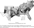
FIGURE 1 WHITE-BLACK LOG EARNINGS GAP, 1939
Perhaps less widely appreciated than the size of the overall racial wage gap is the considerable geographic variation in the gap within the South. Table 1 exhibits the pattern of the gap in mean log weekly earnings between white and black men across southern SEAs in 1939.7
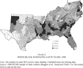
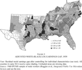
The data used in Figures 1–3 are based on the 1940 IPUMS sample, restricted to adult male workers with fewer than 12 years of education. In these maps the geographical unit is the SEA, so all counties in the same SEA receive the same shading. There are 169 different SEAs represented in these maps. All maps were generated using present-day (c. 2000) county boundaries and Mapland 10 software. Completely unshaded counties had missing or insufficient data (e.g., West Texas and parts of Oklahoma) in Figures 1–3.
Darker areas on the map had a larger gap between white and black wages. The spatial variation is substantial: the SEA at the seventy-fifth percentile had a racial pay gap some 0.31 log points greater than the gap at the twenty-fifth percentile.
Racial inequality in schooling played a role in the spatial pattern of the wage gap, just as it did in the aggregate. Table 2 shows the difference in average years of schooling between white and black adult male workers across SEAs.8
The sample is restricted to individuals with fewer than 12 years of school to be consistent with the sampling criteria used below. The map looks very similar if high-school graduates are included.
Details of the individual log earnings regression used to identify the adjusted wage gap are provided below. For this map, the earnings gap in each SEA is calculated for a hypothetical comparison between a white and a black worker, each 35 years old, married, with eight years of schooling, working in a nonfarm industry, and born in Georgia. Standardizing on a worker with different characteristics would change the levels but not the relative values of the wage gap between SEAs.
In fact, the general spatial pattern of the wage gap is not much altered by controlling for human capital—the correlation between the unadjusted and adjusted racial wage gaps across SEAs is 0.84.

FIGURE 2 WHITE-BLACK SCHOOLING GAP IN YEARS, 1940

FIGURE 3 ADJUSTED WHITE-BLACK LOG EARNINGS GAP, 1939
What can account for the patchwork quilt exhibited in Table 3? If the adjusted wage gap does represent labor market discrimination against African-Americans, what made discrimination relatively severe in some locations and mild in others? To explain these patterns, I begin with a description of how labor market discrimination functioned in the South generally. This discussion points to potential factors influencing equilibrium wage discrimination that varied across the South; these form the independent variables in the empirical analysis that follows.
EXPLAINING THE WAGE GAP AND ITS SPATIAL VARIATION
Wage discrimination in the South was largely the product of a racial division of labor limiting the kinds of jobs open to black workers. These constraints were enforced both by white workers, who resisted competition for preferred jobs and at least some forms of interracial contact, and by white employers' and customers' views regarding the suitability or acceptability of African-Americans for various types of work. Blacks were commonly excluded from supervisory jobs—especially in cases that might involve supervision of whites, which would violate accepted norms of the racial hierarchy; jobs involving substantial interaction with white customers were also often taboo.11
On racial hierarchy, see Dewey, “Negro Employment”; and Sundstrom, “Color Line.”
Examples include obstacles to job promotions in the railroad industry (Sundstrom, “Half a Career”) and racially separate job groupings in the pulp and paper industry (Northrup, “Negro”). Also see Johnson, Patterns.
Spero, and Harris, Black Worker; and Higgs, “Black Progress.”
Black workers' inferior occupational status cannot be fully explained by black deficits in the quantity and quality of schooling.14
Margo, Race.
Wright, Old South.
Higgs, “Firm-Specific Evidence”; and Wright, Old South.
Labor mobility and competition among employers placed limits on discrimination in wages or job assignments. That southern labor was mobile across employers, at least locally, is well known.17
Wright, Old South.
Jones, Dispossessed.
Alston and Kauffman, “Competition.”
Becker, Economics.
Despite these market pressures, there is evidence that by the 1920s a racial wage gap had emerged even in low-skilled markets, where one might expect competition and alternative employment in farming to have had their strongest equalizing effect. Gavin Wright argues that decades of occupational and industrial segregation had resulted in black and white workers occupying “noncompeting jobs,” even at the entry level.21
Wright, Old South, p. 197.
Bergmann, “Effect.” In principle “crowding” could adversely affect the wages of either of the noncompeting groups, but in the case of racial discrimination, mobility was probably asymmetric, with whites able to move into black jobs if increased demand was making the wage attractive, but the reverse less common.
Johnson, Patterns; Donohue and Heckman, “Continuous versus Episodic Change”; and Wright, “Civil Rights Revolution.”
Job search costs give rise to monopsony power in the labor market and the opportunity for employers to wage discriminate against workers with less elastic supply (fewer alternatives): see Manning, Monopsony; Black, “Discrimination”; and Sasaki, “Equilibrium Search Model.”
These general observations suggest four sets of factors that should have determined the degree of wage discrimination in a local labor market: the strength of the racial norms or beliefs that restricted job assignments by race; the relative supply of black versus white workers; the structure of the local job market, in terms of the heterogeneity of demand for skills and the degree of competition; and government interventions in markets that may have constrained wage setting or created temporary disequilibrium. These factors, or observable proxies for them, constitute the explanatory variables I use to predict the adjusted racial wage gap across SEAs.
Racial Attitudes and Norms
White racial attitudes and unwritten social rules governing black-white relations varied considerably across the South. As Charles Johnson put it, “Within the framework and policy of racial segregation are wide variations in local practice.”25
Johnson, Patterns, p. 6.
Alston, “Race Etiquette”; Alston and Ferrie, “Paternalism”; and Wright, “Reflections.”
For the period under study, direct evidence on racial attitudes, such as might be derived from social surveys, cannot be obtained at a useful level of disaggregation.27
In his study of race etiquette and tenancy in the South, Alston (“Race Etiquette”) uses data from a survey of African-Americans from 1961/62. But the timing and small sample sizes of such surveys render them of little utility in the present study.
Virts, “Change.”
Relative Supply of Black Workers
Discrimination in job assignments shaped the relative demand for black versus white labor, which interacted with the relative supply of black and white workers to determine the racial wage differential. Studies going back at least to that of H. M. Blalock tend to find a positive correlation between percent black and the racial income gap, although not always.29
Blalock, “Per Cent Non-White.” See recent studies by sociologists, such as Fossett and Seibert, Long Time Coming; Cohen, “Black Concentration Effects”; and Huffman and Cohen, “Racial Wage Inequality.” Using state-level data for different occupational groupings, Flanagan (“Racial Wage Discrimination”) found no significant effect of relative supply on relative wages for most occupations.
Becker, Economics.
Bergmann, “Effect.”
Thurow, Generating Inequality; and Wright, Old South.
Sociologists refer to the same idea as the “overflow” or “spillover” hypothesis (e.g., see Fossett and Seibert, Long Time Coming).
This is a prediction of search models of discrimination, such as those of Black, “Discrimination”; and Sasaki, “Equilibrium Search Model.” See also Akerlof, “Discriminatory, Status-Based Wages.” Empirical support for such models can be found in Barth and Dale-Olsen, “Monopsonistic Discrimination”; and Bowlus and Eckstein, “Discrimination.”
Racial composition may also have affected racial attitudes or taste for discrimination. A common argument posits that where blacks constituted a larger share of the local population, they were perceived by whites as a greater social, economic, or political threat.35
See, for example, Allport, Nature; Becker, Economics; and Huffman and Cohen, “Racial Wage Inequality.”
Myrdal, American Dilemma; Heer, “Sentiment”; and Tolnay and Beck, Festival.
Spero and Harris, Black Worker.
Whatley, “Getting a Foot.”
Finally, concentration of African-Americans in impoverished southern communities might have operated like residential segregation to create adverse neighborhood or social network effects, as noted by David Cutler and Edward Glaeser.39
Cutler and Glaeser, “Are Ghettos.”
Collins and Margo, “Residential Segregation.”
Assessing the impact of relative supply or proportion black on the relative wage empirically requires dealing with the likely endogeneity of relative supply. To the extent that black workers were mobile and responsive to wage incentives, they would have tended to move from areas with more severe wage discrimination to areas with less. In the presence of a crowding effect, migration that reduced the relative supply of blacks in the place of origin would narrow the wage gap there and increase it in the place of destination. An estimate of the crowding effect based on the correlation between relative supply and relative wages would then be biased toward zero. The evidence summarized in Table 3 provides strong circumstantial evidence that considerable spatial variation in the wage gap survived such labor flows. But mobility between state economic areas in the South was not uncommon: In my core sample of male workers in 1940, 6.3 percent of blacks and 10.7 percent of whites had changed SEA of residence between 1935 and 1940.41
These numbers come from responses to the Census question on residence in 1935, for those individuals in the IPUMS with known SEA in both 1935 and 1940.
Ideally, to identify the direct effect of proportion black on the wage gap one would like to have a natural experiment, a la the Mariel boatlift, that exogenously altered the racial composition of some SEAs.42
See Card, “Impact.”
Job Market Structure
In a homogeneous job market with limited opportunities for skill acquisition, racial job restrictions would have had relatively limited impact on black-white relative wages. Competition among employers for workers would likely have mitigated the effects of taste for discrimination. At the SEA level, available data are inadequate to calculate any sophisticated measures of job heterogeneity or market concentration. Instead, I rely on a few basic controls for economic characteristics of the SEA: proportion of population urban and the proportions of workers employed in manufacturing and in agriculture. Compared with labor markets in rural, agricultural areas, labor demand in urban and industrial areas was likely more diversified in terms of occupations and skills, with correspondingly greater potential for restrictions on skill acquisition; more differentiated markets may also have created opportunities for the exercise of market power against black workers by employers or organized white workers with specialized skills.43
For restrictions on skill acquisition, see Fossett and Seibert, Long Time Coming, p. 65.
Government Policy
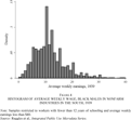
Measuring the impact of labor-market discrimination within the South in 1940 is complicated by federal policies of the period that may have generated long-run or short-run disequilibrium conditions in the labor market: namely, the minimum wage and agricultural adjustment policies. To the extent that the legal minimum wage established under the Fair Labor Standards Act of 1938 was enforced and binding, it would have forced racial wage equality in the lower tail of the distribution in covered sectors of the economy. In this case, employers with a taste for discrimination would simply have failed to employ black workers, forcing them into nonemployment or the uncovered sector (predominantly agriculture). The measured racial wage gap among employed workers in nonfarm industries would then be biased toward zero in low-wage areas.
Studies by the Bureau of Labor Statistics at the time suggested that the minimum wage was much more likely to be binding in the low-wage South than elsewhere in the country.44
U.S. Dept. of Labor, Labor; Schulman, From Cotton Belt, p. 66; see also Cogan, “Decline.”
Industries that could claim not to be engaged in interstate commerce—such as some sawmills, for example—were not covered by the FLSA, which along with lax enforcement may help explain the presence of subminimum pay in the figure (see Schulman, From Cotton Belt). The minimum was raised to 30 cents per hour effective 24 October 1939.

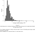
FIGURE 4 HISTOGRAM OF AVERAGE WEEKLY WAGE, BLACK MALES IN NONFARM INDUSTRIES IN THE SOUTH, 1939

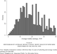
FIGURE 5 HISTOGRAM OF AVERAGE WEEKLY WAGE, BLACK MALES IN FARM INDUSTRIES IN THE SOUTH, 1939
Because the legal minimum was of course a uniform federal policy across locations, its impact on the wage racial gap cannot be estimated directly from cross-section data. Rather, in results discussed below, I examine the potential impact of the minimum wage on my results by estimating the model for a sample restricted to workers with above-minimum earnings, correcting for the selection bias. The main results are robust to this specification.
New Deal farm policy may also have had at least a short-run effect on the geographical pattern of the racial wage gap. The shift from sharecropping to wage labor and the mechanization of preharvest activities in response to incentives created by the Agricultural Adjustment Act resulted in a release of tenants into the wage-labor market, but with little immediate out-migration until the wartime increase in demand for industrial labor.46
Whatley, “Labor.”

FIGURE 6 HISTOGRAM OF AVERAGE WEEKLY WAGE, WHITE MALES IN NONFARM INDUSTRIES IN THE SOUTH, 1939
EMPIRICAL MODEL OF THE RACIAL EARNINGS GAP
To identify empirically the covariates of wage discrimination across southern SEAs, I employ a two-stage regression procedure. The first stage is a log earnings regression using individual-level census data, with controls for individual characteristics, including age, education, and marital status, a set of state economic area (SEA) dummy variables, and interactions of those SEA variables with a dummy for white race. The coefficients on the SEA-race interactions represent estimates of the white earnings premium or racial earnings gap (in log points) within each SEA, adjusted for racial differences in skills and returns to skill. That is, the adjusted racial earnings gap by SEA j is a set of coefficients (φj) on interactions between race and SEA dummy variables:

where yi is log earnings for individual i, Xi is a vector of individual characteristics, di is a dummy variable equal to one for whites and zero for blacks, and Zj is a dummy variable equal to one for SEA j. This specification allows the returns to the human capital variables X to differ by race but constrains them to be the same across all SEAs.
47Estimating a fully interacted model in which the returns to X variables are SEA-specific is hampered by sample-size limitations, although I report some results for such an exercise below.
In the second stage, the estimated interaction coefficients

are regressed on characteristics of the SEA, Sj

Because of sampling error in the estimation of φj, the errors of the second-stage regression ej are heteroskedastic, so I use the estimated standard errors from the first stage to form weights for weighted least squares.
48Following a similar strategy employed by Card and Krueger, “School Quality,” observations are weighted by the inverse of the squared standard error. This is only approximately correct, because the second-stage error variances should include not only a measurement error but also a model error component, and are in principle correlated with each other off the diagonal.
Census Earnings Data and First-Stage Regressions
Any effort to analyze earnings across local labor markets in the South prior to the modern Civil Rights movement of the 1960s is hampered by data limitations. Blalock used 1950 Census data on black-white income differences at the county level to show that the racial income gap was greater in counties with a larger proportion black.49
Blalock, “Per Cent Non-White.”
The federal census did not collect information on educational attainment or earnings before 1940, so standard controls for individual skills cannot be employed until that date. Earnings and education were only asked of a subsample of respondents to the 1950 Census (sample line individuals), limiting the number of observations available within small geographical units. The microsample of the 1960 Census does not identify any geographical unit smaller than the state. This leaves one with the 1940 Census, which includes earnings and education information, and for which the smallest identifiable geographical unit is the SEA.50
Ruggles et al., Integrated Public Use Microdata Series.
One potential concern about relying on the 1940 census is that 1940 was not a very typical year because of the lingering impact of the Great Depression. Nationwide, substantial numbers of workers remained unemployed or on government-sponsored work relief programs, such as the WPA, and therefore those workers reporting earnings may have been a selective group.51
Unemployed and emergency workers are not included in the regression samples discussed below.
See Sundstrom, “Explaining the Racial Unemployment Gap.”
For the first-stage (log earnings) regression, the sample consisted of all individuals in the 1940 IPUMS satisfying the following criteria: white or black male, age 18–64; fewer than 12 years of education completed; wage or salary worker; holding civilian job; worked at least 26 weeks during 1939; positive earnings in 1939; and residing in southern SEA with at least five white and five black workers satisfying the preceding criteria. This sample contained 11,560 blacks and 27,585 whites.
In 1940 only a small fraction of southern blacks had completed high school (6.7 percent of the black workers satisfying my other sampling criteria), whereas a substantially larger proportion (33.3 percent) of whites had. To the extent that a high-school diploma opened up a range of job opportunities generally unavailable to less-educated workers, high-school graduates occupied a distinct segment of the labor market from which most blacks were excluded. For the purposes of identifying labor-market discrimination, then, restricting the sample to workers who had not finished high school yields a sample of whites who are more comparable with the vast majority of black workers.53
The core results presented below are robust to including high-school grads in the sample. This and other sensitivity checks reported in the article are available from the author upon request.
The dependent variable for the earnings regression is the natural log of average weekly earnings in 1939, calculated as wage and salary income for 1939 divided by weeks worked in 1939. The 1940 census only reported total wage and salary earnings and total weeks worked for the preceding year, not total hours or hourly wages. However, the weeks worked question in the 1940 census asked respondents to report their estimated 1939 full-time equivalent workweeks, typically normed to a 40-hour workweek. Thus an individual who worked 50 weeks at 20 hours per week was expected to report 25 weeks. This procedure implies that the weeks worked are really an estimate of total hours / 40, so the average weekly earnings measure used here is roughly proportional to average hourly earnings.
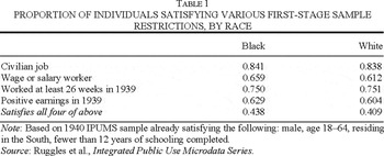
Table 1 shows the proportion of individuals satisfying the various work-related sample restrictions, conditional on less than high school completion, by race. Altogether, only about two-fifths of the observations satisfy all the restrictions, but the degree of selectivity is very similar for blacks and whites. The sampling criteria for valid weekly earnings disproportionately exclude individuals working in farming, because a large fraction of farmers and farm workers were owners or tenants rather than wage or salary workers. Among whites, the sampling criteria exclude 46 percent of individuals in nonfarm industries, but fully 86 percent of those in farm industries. The corresponding numbers for blacks are 43 and 74 percent.

Southern farm workers often received some of their payment in kind.54
See Alston and Ferrie, “Labor Costs.”
In the earnings regressions, the basic individual controls (Xi) are for age, education, agricultural industry, and marital status (married with spouse present). All are fully interacted with race to allow for racial differences in returns. Age is entered as a quadratic and education is linear in years of schooling completed.55
This specification closely follows the standard Mincer earnings regression format. Heckman et al. (“Fifty Years”) have shown that the key assumptions of the Mincer specification hold up fairly well for the 1940 and 1950 census data (although not so well in more recent years). I use age and its square in place of the conventional measure of potential experience (equal to age minus years of school minus six) and its square. The standard experience measure seems suspect in my sample, in which a large percentage of workers have very few years of schooling (the median for blacks is five years). According to the conventional experience calculation this would count work at age 11 or even younger as work experience for a good many individuals. No doubt many children were working in the South, but whether their experience contributed to human capital acquisition in the same way as a young adult's is open to question. At any rate, figures in Heckman et al., “Fifty Years,” show that the age and experience profiles of earnings, stratified by schooling, actually have quite similar shapes in 1940. Using potential experience in place of age does not substantively change my results.
Complete first-stage regression results are available from the author upon request.
Card and Krueger, “School Quality.”
These data were kindly provided by Carolyn Moehling. Because it is impossible to know where an individual was living when he received his education, each was assigned the school quality proxies for his 1940 SEA of residence. The 1940 Census did record state of birth, and I restricted this sample to those individuals residing in their state of birth to reduce potential measurement error introduced by migration between schooling and 1940.
The earnings regressions do not include controls for occupation. To the extent that wage discrimination operated through differential job assignments that created obstacles to black advancement, controlling for occupational status would simply remove a key component of wage discrimination from the SEA wage gap estimates. Racial differences in occupational assignments that resulted from black deficits in the quantity and quality of schooling, on the other hand, should be captured by the educational controls in the earnings regression.
SEA-Level Data
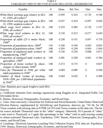
The objective of the second-stage regressions is to estimate the impact of local labor-market (SEA) characteristics (Sj) on the SEA white-black earnings premium estimated in the first stage. Regressors were chosen based on the theoretical and historical factors discussed in the preceding section and were in each case generated by aggregating county data to the SEA level. Summary statistics for the independent and dependent variables in the SEA sample are given in Table 2. The first two variables represent the adjusted racial wage gap as estimated by the coefficient on the white-SEA interaction in the first-stage log earnings regression, relative to the excluded SEA category.59
The excluded SEA is ICPSR SEA#1, consisting of the Alabama counties of Colbert, Lauderdale, Lawrence, Limestone, Madison, and Morgan.
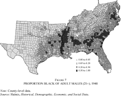
The relative supply of black workers in the SEA is measured as the proportion black among adult males (21 and over). The sign of the coefficient on proportion black should depend on the offsetting effects of crowding and upgrading on black wages, as discussed previously. The mean of proportion black indicates that about a quarter of the adult male population was black in the average southern SEA. The spatial distribution of proportion black (by county) is illustrated in Table 7; it exhibits the expected concentration of blacks in the southern “black belt” areas. Comparing Figures 3 and 7, the spatial correlation between the earnings gap and relative supply appears to be positive, but is far from perfect.


FIGURE 7 PROPORTION BLACK OF ADULT MALES (21+), 1940
Two variables are included as measures of prosegregationist or antiblack behavior by whites: the number of votes for Strom Thurmond in the 1948 presidential election per white adult population, and the number of black victims of known lynchings during the period 1910–1930 per 1,000 black population. Thurmond was the candidate of the explicitly segregationist “Dixiecrat” movement in the South.60
Key, Southern Politics, chap. 15.
Heer, “Sentiment.”
An additional variable that may proxy for local racial attitudes is the prevalence of plantations, measured here as the proportion of farms worked by sharecroppers or share tenants. Nancy Virts suggests that sharecropping is probably the best proxy for plantation agriculture for this period, although I obtain similar results using plausible alternative measures, such as the value of the cotton crop per capita.62
Virts, “Change.”

Finally, some basic controls for economic characteristics of the SEA are included, which are intended to pick up some of the impact of the local job structure and competition on measured discrimination: the proportion of population urban and the proportions of workers employed in manufacturing and in agriculture. I use the census definition of urban places—namely places with population at least 2,500—but the results are not substantively different if an urban control for population in places of 25,000 or greater is added.
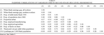
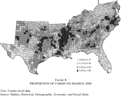
Table 3 presents correlations between the various SEA-level variables used here. Notable are the positive correlations between the racial earnings gap on the one hand and the proportion black, the proportion of farms operated on shares, and the Thurmond vote on the other. These correlations suggest the potential roles of relative supply, plantation institutions, and white racial attitudes in generating wage inequality. But these variables are also correlated with one another. For example, comparing Table 7 with Table 8, which shows the proportion of farms on shares, indicates unsurprisingly that the “black belt” coincided to some degree with the “plantation belt.” A multiple regression approach is needed to sort out the distinct partial effects.
RESULTS
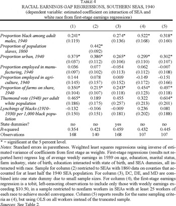
The second-stage regression results for 1940 are reported in Table 4. In the core specification, presented in column (1), the coefficients on proportion black, proportion urban, sharecropping, and proportion of votes for Thurmond are all positive and statistically significant. Among these variables, the urbanization effect is strongest: a one standard deviation increase in proportion urban increases the adjusted log racial wage gap by about 0.09, or nearly half a standard deviation of the dependent variable. The effects of proportion black and sharecropping are more modest but still substantial: a one standard deviation increase widens the wage gap by about 0.04 and 0.06 respectively. The results are not substantively changed when the first-stage regression is restricted to nonfarm workers (not reported here).63
The core results presented in Table 4 are also robust to a variety of alternative specifications. For example, adding variables for the proportion of population in larger cities (25,000 plus) and the value of the cotton crop per capita to provide a richer specification of urbanization and patterns of agriculture does not alter the main results (neither of these additional variables is significant). In another specification, I interacted the Thurmond variable with state dummies for Alabama, Louisiana, Mississippi, and South Carolina, the states where Thurmond was listed on the ballot as the official candidate of the Democratic Party and might therefore have received more votes from party-line voters. This did not alter the basic results. Finally, the results are also robust to estimating the first-stage earnings regressions using quantile (median) regression rather than OLS as a means of mitigating the impact of potential outliers in small SEA cells. All alternative results are available from the author upon request.

FIGURE 8 PROPORTION OF FARMS ON SHARES, 1940
As noted, the coefficient on proportion black is likely to be biased due to endogenous migration, which would be expected to mitigate the crowding effect on wage discrimination. Column (2) reports the results of a reduced-form equation replacing the proportion black variable with the proportion of the SEA population in 1860 who were slaves, which is highly correlated with proportion black in 1940 but should be exogenous to the 1940 wage gap. The coefficient on the slavery variable in column (2) is large and significant: a one standard deviation increase in the proportion slave in 1860 is associated with an increase in the 1940 racial wage gap of nearly one-half standard deviation.64
The sample used in estimating column (2) is restricted to SEAs in which the counties with valid 1860 data make up at least half the SEA population in 1940. When the regression specification from column (1) is estimated for this restricted sample, the coefficient on proportion black in 1940 rises to 0.328.
IV results are available from the author upon request. The 1860 slavery variable is a strong instrument, with an F statistic in the first-stage regression of 131.7. As suggested, however, it may not be a valid instrument, given the likely correlation between historical slave districts and other, unobserved local characteristics.

To the extent that the positive coefficient on proportion black represents the genuine effect of racial composition on the wage gap, it suggests that the job-market crowding and threat effects of increased relative supply of black workers in a local market dominated any offsetting tendency toward occupational upgrading. Of the two fairly direct proxies for racial attitudes—the Thurmond vote and lynching variables— only the Thurmond variable is significantly different from zero, and not in every specification. The significant coefficient on the plantation proxy (sharecropping), which is robust even after controlling for the overall importance of agriculture in the local economy, may be a better indication that local social relations, including white racial attitudes, affected black labor-market opportunity. Finally, the positive coefficient on urbanization is consistent with the hypothesis that the more heterogeneous structure of urban job markets created more opportunities for discrimination in job assignments. The finding that both urbanization and sharecropping are associated with a larger racial wage gap, ceteris paribus, is less paradoxical than it may appear. Sharecropping SEAs were more likely to be rural, but the correlation of –0.45 (see Table 3) between proportion urban and proportion of farms on shares is far from perfect, allowing the regression to identify separate marginal effects of these variables.
Alternative Specifications and Samples
Column (3) of Table 4 repeats the specification of column (1) but adds a set of state dummies as a control for unmeasured factors across larger geographic units, such as the potentially more relaxed race relations in the border states. Unsurprisingly, inclusion of state dummies tends to weaken some of the estimated coefficients, but the results are overall qualitatively similar.
The results in column (4) attempt to correct for potential bias created by the federal minimum wage. As noted, if the minimum wage were binding on workers of both races, it would tend to obscure the racial wage differential in low-wage markets. This could bias toward zero the estimated coefficients on any SEA characteristics that were correlated with both the racial wage gap and low wages overall. To address this problem, I have estimated the first-stage log earnings equation as a tobit, censoring all observations with weekly earnings at or below $10.50, a figure slightly above the average weekly earnings a full-time worker would have earned at the minimum wage in 1939, and just above the observed spike in the black earnings distribution in Table 4. In this case, the parameters of the earnings equation are estimated from the observations with earnings above the minimum, correcting for the potential bias due to censoring. The data are restricted to nonfarm workers, because agriculture was not generally covered by the minimum.66
To achieve convergence of the tobit model required limiting the number of SEA dummies estimated, which I accomplished by restricting the sample to those SEAs with at least 25 observations of each race.
Another potential source of bias in the results is the possibility that the SEA characteristics associated with a larger racial wage gap are merely picking up the indirect effect of unobserved worker productivity differences. For example, perhaps my controls for school quality fail to capture fully the extent to which schooling for blacks was particularly bad in areas of concentrated black population. If unobserved school quality were driving the results, one would expect to find that the same variables found to influence the racial gap in earnings would also significantly affect the estimated returns to schooling across SEAs. In regression results not presented here, I find little evidence that this is the case.67
The racial gap in returns to schooling by SEA can be estimated by interacting years of schooling with SEA and race in the first-stage regression. The second-stage regression of these estimates on the regressors used in Table 4 fits quite poorly; only the Thurmond vote variable has a significant (positive) coefficient. Results are available from the author.
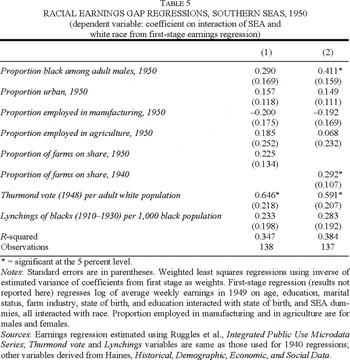
As a further check on the robustness of the results presented in Table 4, I have estimated the same model using census data from 1950, to make sure the 1940 results are not merely the product of an abnormal census year. The second-stage results are presented in Table 5. The sample is somewhat smaller than for 1940, because earnings and education information is available for only a subset of the 1950 IPUMS sample, so fewer SEAs meet the minimum sample threshold. In column (1), all the regressors that can be are updated to 1950 values (the exceptions being the Thurmond vote and lynching variables). The coefficient on proportion black is similar in magnitude to its value for the 1940 sample, although it is only marginally statistically significant (p-value of 0.09). The proportion urban coefficient is again positive, but smaller and not statistically significant. In comparison with the 1940 results, the impact of the sharecropping variable in 1950 is smaller and weakly significant. Sharecropping was in decline during the 1940s, spurred by the AAA and mechanization: between 1940 and 1950, the percentage of farms operating on shares in the average SEA in my samples fell from 27 to 20. But the former plantation districts apparently retained their tendency toward a larger wage gap. This can be seen in column (2) of Table 5, which replaces the 1950 values of the sharecropping variable with the 1940 values. Here, the estimated coefficient on sharecropping is quite similar to its value in Table 4 (positive and significant). Clearly the 1940 sharecropping variable proxies for some more persistent underlying characteristic of these plantation areas.

Variation in Black and White Wage Levels Across SEAs
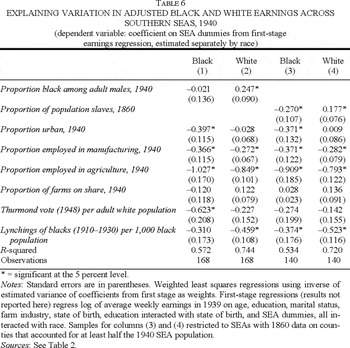
The primary focus of this article has been on the adjusted racial earnings gap, interpreted as a measure of labor-market discrimination. Of course the wage gap could be larger as a consequence of white wages being higher, black wages being lower, or some combination of the two. Using the first-stage regression results, we can examine geographic variation in the adjusted earnings levels of black and white workers, controlling for individual measured human capital and the racial wage gap. The estimated coefficient on a specific SEA dummy variable captures the difference between black earnings in that SEA and black earnings in the excluded SEA category, whereas the analogous difference in white earnings is the sum of the coefficients on SEA and the SEA * white interaction.68
For convenience in obtaining the estimated standard errors for the white earnings levels, I estimated the first-stage regression again with whites as the excluded category and used the SEA coefficients as estimates of the white wage levels.
Estimates for nonfarm workers only were similar to those reported in Table 7.
Comparing the effect of proportion black on the earnings levels of blacks versus whites, it can be seen that an increase in the relative supply of black workers tended to have little effect on black wages and to increase white wages. Urbanization depressed black wages, with no significant impact on white wages. For both races, earnings were negatively related to agricultural and manufacturing employment and to the lynching rate, but in each case the difference between the black and white coefficients was not large enough to have a significant impact on the racial wage gap in Table 4. These results suggest that the local factors correlated with general poverty, as measured by low wages for both whites and blacks, were not necessarily the same factors affecting the racial pay gap.
Columns (3) and (4) of the table replace the contemporaneous racial composition with the proportion slaves in 1860. Blacks residing in former slave areas earned lower wages in 1940, while whites in the same areas earned significantly higher wages. These results indicate that, ceteris paribus, white workers could have earned more by moving into traditionally black areas, whereas black workers could have earned more by leaving them. That migration within the South did not redistribute population in such a way as to equalize returns for each race echoes the familiar North-South regional wage gap; but obviously some of the important explanations for the latter, such as the general isolation of southern labor markets or the competition that blacks faced from low-skilled European immigrants, are not plausible for the within-South case.70
On the general isolation of southern labor markets, see Wright, Old South. On competition from immigrants, see Collins, “When the Tide.”

CONCLUSIONS
Black workers in the South were paid substantially lower wages than their white counterparts, even after controlling for a range of individual characteristics. Furthermore, this wage differential varied considerably across location within the South. A robust and striking finding of this article is that the racial pay gap was substantially greater in local labor markets with a greater relative supply of black workers (proportion black). This geographical pattern was apparently a long-run legacy of the geographical distribution of slavery: the distribution of slaves per capita in 1860 is an even better predictor of the 1940 wage gap than is the contemporaneous distribution of blacks. The pay gap also tended to be greater in more urbanized SEAs, in plantation districts, and in areas where whites revealed segregationist preferences in the 1948 presidential election. Overall, the results are consistent with the picture that wage discrimination was generated by restrictions on the labor-market opportunities open to blacks. In historically black areas of the South, labor-market crowding reinforced traditional racial norms and white hostility, to the disadvantage of black workers.
At first glance the regression results seem to suggest a potential factor contributing to declining discrimination in the South after 1940: out-migration of blacks reduced their relative numbers and thus may have relieved some of the market and social pressures that exacerbated wage discrimination. The problem with such a hypothesis is the timing. The net migration of blacks out of the South was largely over by the mid-1960s, whereas rapid wage convergence within the South was a product of the post-1965 period. But perhaps the adjustments to the changes in relative supply that accompanied the Great Migration—particularly those relating to racial norms and perceptions of threat or competition—occurred with a lag.
Southern society confronted African-Americans with a web of social and economic restrictions. In such an environment, increased relative numbers could actually make matters worse by increasing the competition for limited opportunities. In another context, increased numbers might have offered an alternative avenue toward improvements in status through the exercise of political power; but this route was blocked until the advances in black political rights of the 1960s.
I am grateful to Carolyn Moehling for insightful comments on an earlier draft and for providing access to her county-level school quality data. I also thank Lee Alston, Marianne Page, Gavin Wright, and two anonymous referees for very helpful suggestions. Partial financial support was received from a Breetwor Fellowship, Leavey School of Business, Santa Clara University.