1 Introduction
Biomembrane is mainly composed of the lipid-bilayer membrane with fluidity and is surrounded by aqueous environments. It contains various lipids, carries various membrane proteins and is combined with glycocalyx and cytoskeleton (Alberts et al. Reference Alberts, Johnson, Lewis, Raff, Roberts and Walter2007). To elucidate its physical properties, many researchers have studied simpler model membranes experimentally and theoretically. Studies on the phase separation on a vesicle of ternary mixture of phospholipids and cholesterol (Dietrich et al. Reference Dietrich, Bagatolli, Volovyk, Thompson, Levi, Jacobson and Gratton2001; Veatch & Keller Reference Veatch and Keller2002, Reference Veatch and Keller2005) were originally triggered by the raft hypothesis (Simons & Ikonen Reference Simons and Ikonen1997), which asserts that microdomains of ten to several hundreds of nanometres in size, enriched in specific lipids, should give platforms for biochemical reactions in the biomembrane. It was found that the critical exponents of this phase separation on the artificial membrane agree with those of the two-dimensional (2-D) Ising model (Honerkamp-Smith et al. Reference Honerkamp-Smith, Cicuta, Collins, Veatch, den Nijs, Schick and Keller2008) and that the dynamic critical exponent shows the cross-over from the value of a 2-D system to that of a three-dimensional (3-D) system as the membrane approaches the critical point (Inaura & Fujitani Reference Inaura and Fujitani2008; Honerkamp-Smith, Machta & Keller Reference Honerkamp-Smith, Machta and Keller2012; Fujitani Reference Fujitani2013c ). Domain coarsening in the phase separation has also been found to have characteristic growth rates and to be accompanied by the shape deformation of the membrane (Yanagisawa et al. Reference Yanagisawa, Imai, Masui, Komura and Ohta2007). Thus, the multicomponent fluid membrane is an interesting object in the field of soft matter physics apart from the biological relevance; various phenomena occur in an apparently 2-D fluid in contact with 3-D fluids.
Let us consider a colloidal sphere immersed in a 3-D fluid. The force which the ambient fluid exerts on the sphere in its stationary translational motion has a magnitude proportional to the speed if the motion is sufficiently slow. The constant of proportionality is referred to as the drag coefficient, of which reciprocal is thought to give the diffusion coefficient after being multiplied by the Boltzmann constant and temperature (Einstein Reference Einstein1905; Sutherland Reference Sutherland1905; Bian, Kim & Karniadakis Reference Bian, Kim and Karniadakis2016). The drag coefficient of a rigid sphere is known as Stokes’ law (Stokes Reference Stokes1851), while that of a droplet is also well known (Hadamard Reference Hadamard1911; Rybczynski Reference Rybczynski1911; Clift, Grace & Weber Reference Clift, Grace and Weber1978; Loth Reference Loth2008). The latter tends to the former as the viscosity of the droplet increases with the other conditions being kept the same. It is to be noted that we need not consider droplet deformation in calculating the drag coefficient, which is defined in the linear regime. Recently, fluctuation of a colloidal particle can be measured with high resolution in space (
 ${<}1~\text{nm}$
) and time (
 ${<}1~\unicode[STIX]{x03BC}\text{s}$
) (Franosch et al.
Reference Franosch, Grimm, Belushkin, Mor, Foffi, Forró and Jeney2011; Grimm, Franosch & Jeney Reference Grimm, Franosch and Jeney2012), and a Brownian particle is used as a probe for local environments in the field of microrheology (Waigh Reference Waigh2005; Bertseva et al.
Reference Bertseva, Grebenkov, Schmidhauser, Gribkova, Jeney and Forró2012; Grebenkov et al.
Reference Grebenkov, Vahabi, Bertseva, Forró and Jeney2013).
In the biomembrane, the diffusion of membrane proteins is biologically significant. Saffman & Delbrück (Reference Saffman and Delbrück1975) and Saffman (Reference Saffman1976) considered a small rigid disk in a flat 2-D incompressible fluid surrounded by 3-D incompressible fluids and calculated its drag coefficient. It was shown there that the 2-D Stokes paradox (Lamb Reference Lamb1932) is avoided by the momentum flux into the surrounding 3-D fluid. The drag coefficient of a rigid disk of any size was later calculated by Hughes, Pailthorpe & White (Reference Hughes, Pailthorpe and White1981). Some experimental results on a protein or a protein-like inclusion can be explained by this simple model (Peters & Cherry Reference Peters and Cherry1982; Klingler & McConnell Reference Klingler and McConnell1993; Lee & Petersen Reference Lee and Petersen2003; Camley & Brown Reference Camley and Brown2014). Some deviations from this model have also been pointed out in Gambin et al. (Reference Gambin, Lopez-Esparza, Reffay, Sierecki, Gov, Genest, Hodges and Urbach2006), Guigas & Weiss (Reference Guigas and Weiss2006), Quemeneur et al. (Reference Quemeneur, Sigurdssone, Renner, Atzberger, Bassereau and Lacoste2014), which means that some of the complexity of the biomembrane can be elucidated by using the exact result of the simple model as a benchmark.
In the phase separation mentioned above, when the artificial membrane lies in the coexistence phase sufficiently far from the demixing critical point, a domain of the dispersed phase takes a circular shape because the line tension is sufficiently large (Honerkamp-Smith, Veatch & Keller Reference Honerkamp-Smith, Veatch and Keller2009). Koker (Reference De Koker1996) calculated the drag coefficient of a circular domain by using Saffman & Delbrück’s model with a rigid disk replaced by a circular liquid domain and by assuming that the membrane viscosity inside the domain
 $(\unicode[STIX]{x1D702}_{i})$
is the same as the one outside the domain
 $(\unicode[STIX]{x1D702}_{o})$
. As compared with the drag coefficient of this domain, the relative drag coefficient of the disk with the same size, depending on the viscosity coefficients involved, is approximately 114 % at the largest. Cicuta, Keller & Veatch (Reference Cicuta, Keller and Veatch2007) measured the diffusion of a circular liquid domain and analysed their data in terms of the benchmark model for a rigid disk. For a theoretical support of this analysis and for possible measurements with high resolution in the future, the drag coefficient should be calculated for a liquid domain with
 $\unicode[STIX]{x1D702}_{i}\neq \unicode[STIX]{x1D702}_{o}$
. The result will help as a benchmark in extracting some information from future experimental data. The drag coefficient of a circular liquid domain was studied for
 $\unicode[STIX]{x1D702}_{i}\neq \unicode[STIX]{x1D702}_{o}$
in Aliaskarisohi et al. (Reference Aliaskarisohi, Tierno, Dhar, Khattari, Blaszczynski and Fischer2010), Fujitani (Reference Fujitani2013a
), Rao & Das (Reference Rao and Das2015). However, no results have shown that the drag coefficient of a circular liquid domain changes from the result of Koker (Reference De Koker1996) to the one of Hughes et al. (Reference Hughes, Pailthorpe and White1981) as
 $\unicode[STIX]{x1D702}_{i}$
increases from
 $\unicode[STIX]{x1D702}_{o}$
to infinity.
In this paper, we consider Saffman & Delbrück’s model with a rigid disk replaced by a circular liquid domain having arbitrary membrane viscosity and calculate the drag coefficient of the domain. One boundary condition has a distinctive feature originating from the contact of the 2-D and 3-D fluids, as was pointed out in Fujitani (Reference Fujitani2013a
). When
 $\unicode[STIX]{x1D702}_{i}\neq \unicode[STIX]{x1D702}_{o}$
, the continuity of the stress makes the velocity gradient discontinuous across the domain perimeter in the membrane. On the other hand, the velocity gradient is continuous in the ambient fluids, whose velocity field should agree with that of the membrane as the spatial point approaches the membrane. The usual procedure of solving the governing equations without considering the stress continuity across the domain perimeter still leads to a definite solution, which is correct only when
 $\unicode[STIX]{x1D702}_{i}=\unicode[STIX]{x1D702}_{o}$
. This point is also mentioned later in the present study. We introduce a dimensionless parameter,
 $$\begin{eqnarray}\displaystyle \unicode[STIX]{x1D705}\equiv 1-\frac{\unicode[STIX]{x1D702}_{o}}{\unicode[STIX]{x1D702}_{i}}, & & \displaystyle\end{eqnarray}$$
which vanishes in the case studied in Koker (Reference De Koker1996) and approaches unity as
 $\unicode[STIX]{x1D702}_{i}$
increases to infinity. In Fujitani (Reference Fujitani2011), the drag coefficient was calculated up to the linear order with respect to
 $\unicode[STIX]{x1D705}$
, but the stress continuity mentioned above was overlooked. This error was corrected and the drag coefficient was recalculated up to the same order of
 $\unicode[STIX]{x1D705}$
in Fujitani (Reference Fujitani2013a
). In the present study, considering the boundary condition properly, we obtain the drag coefficient of a liquid domain in terms of the infinite series with respect to
 $\unicode[STIX]{x1D705}$
. We derive the recurrence relation for the coefficients of the series, which involves various integrals over infinite intervals to be calculated numerically. Using a truncated series, which gives a good approximation to the sum of the infinite series, we show how the drag coefficient changes from the result of Koker (Reference De Koker1996) to the one of Hughes et al. (Reference Hughes, Pailthorpe and White1981) as
 $\unicode[STIX]{x1D705}$
increases from zero to unity. The drag coefficient of a circular liquid domain is calculated by using the same model as ours in Rao & Das (Reference Rao and Das2015), where the uncorrected boundary condition of Fujitani (Reference Fujitani2011) was somehow used although Fujitani (Reference Fujitani2013a
) was cited.
Our formulation is stated in § 2, and some previous results are shown in § 3. Most parts of the procedure in these sections are the same as given in Fujitani (Reference Fujitani2013a ); we show some equations indispensable for this paper to be self-contained in these sections. See appendix A for details. Our results are shown in § 4, and some details are relegated to appendices. The final section is devoted to discussion.
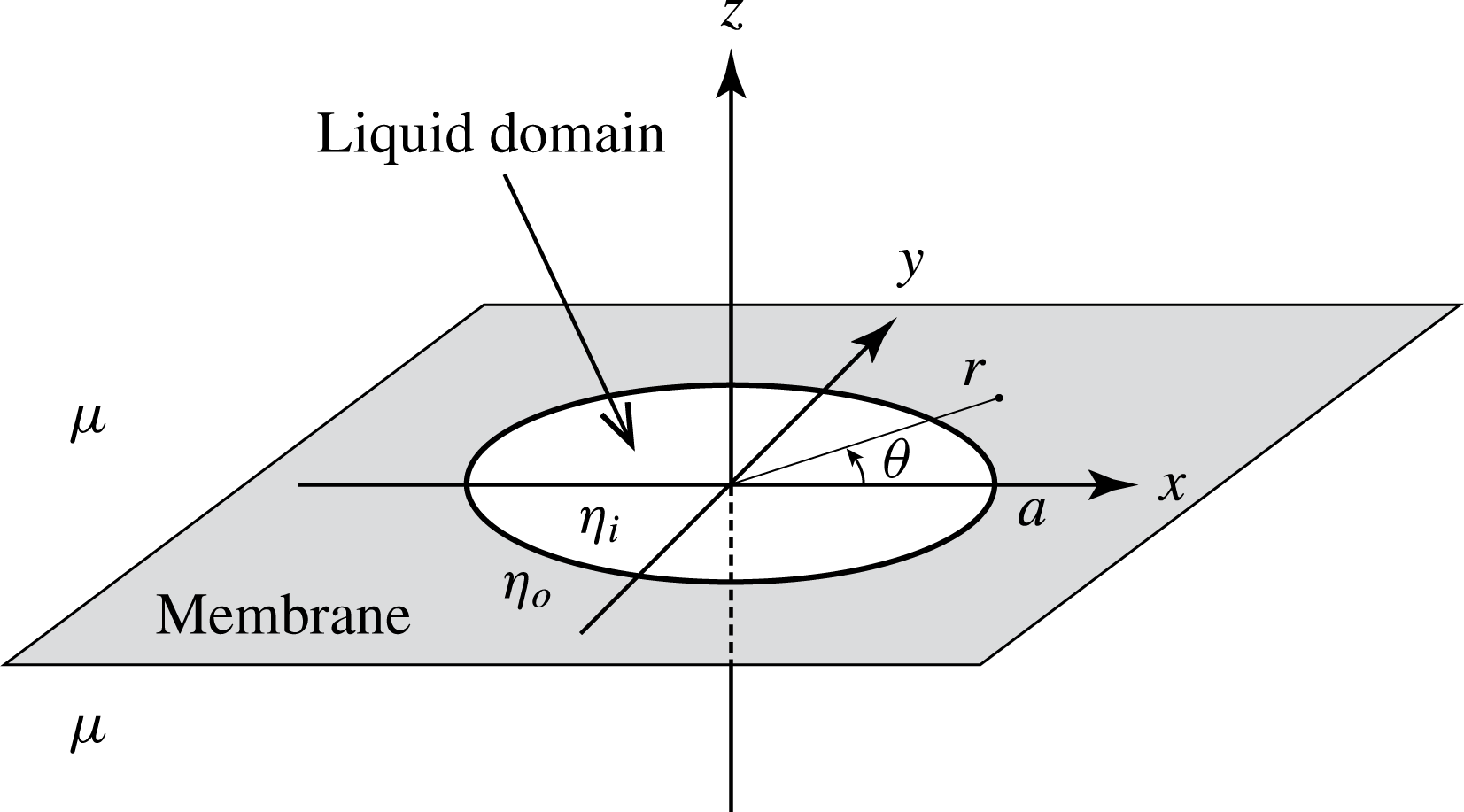
A circular liquid domain with radius
 $a$
and viscosity
 $\unicode[STIX]{x1D702}_{i}$
is embedded in a fluid membrane stretching on the
 $xy$
-plane infinitely. The membrane viscosity outside the domain is denoted by
 $\unicode[STIX]{x1D702}_{o}$
. The semi-infinite spaces on both sides of the membrane are filled with 3-D fluids sharing the same viscosity
 $\unicode[STIX]{x1D707}$
.

2 Formulation
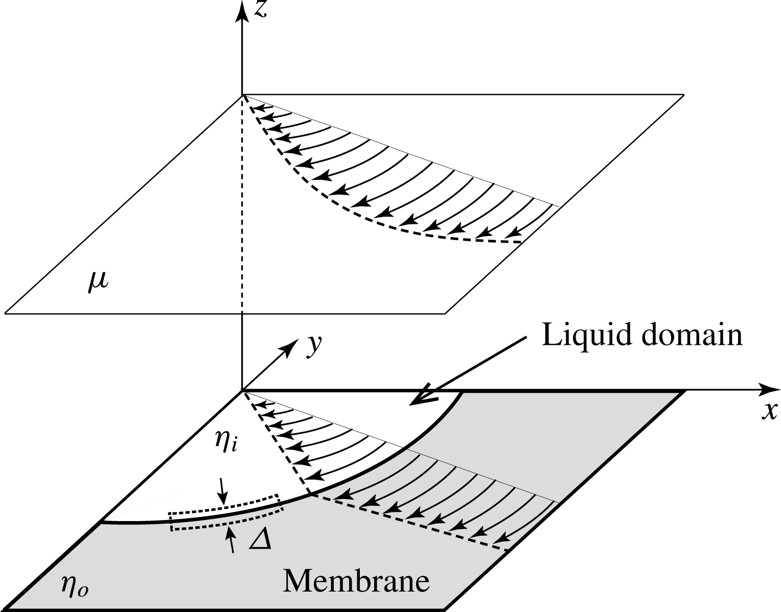
As is shown schematically in figure 1, the membrane is assumed to lie on the
 $xy$
-plane of the Cartesian coordinate system
 $(x,y,z)$
. We also set the cylindrical coordinates
 $(r,\unicode[STIX]{x1D703},z)$
so that the line
 $\unicode[STIX]{x1D703}=0$
is the
 $x$
-axis. A circular liquid domain with the radius
 $a$
shifts translationally with the velocity
 $\boldsymbol{U}=U\boldsymbol{e}_{x}$
, where
 $\boldsymbol{e}_{x}$
denotes the unit vector along the
 $x$
-axis. We consider the instant when the centre coincides with the origin. The 3-D fluids on both sides of the membrane share the same viscosity
 $\unicode[STIX]{x1D707}$
. On the liquid domain, the forces are exerted by the ambient 3-D fluids on both sides of the membrane and by the 2-D fluid outside the domain. The drag force can be written as
 ${\mathcal{F}}_{x}\boldsymbol{e}_{x}$
, and the drag coefficient
 $\unicode[STIX]{x1D6FE}$
is given by
 $-{\mathcal{F}}_{x}/U$
.
The velocity field in the 3-D fluids and that of the fluid membrane are respectively denoted by
 $\boldsymbol{V}$
and
 $\boldsymbol{v}$
. The 3-D velocity field satisfies the Stokes equation and the incompressibility condition,
 $$\begin{eqnarray}\displaystyle \unicode[STIX]{x1D707}\unicode[STIX]{x0394}\boldsymbol{V}=\unicode[STIX]{x1D735}P\quad \text{and}\quad \unicode[STIX]{x1D735}\boldsymbol{\cdot }\boldsymbol{V}=0, & & \displaystyle\end{eqnarray}$$
where
 $P$
denotes the pressure field. Equation (2.1) holds for
 $z\neq 0$
. The 2-D velocity field of the membrane fluid also satisfies the Stokes equation and the incompressibility condition,
 $$\begin{eqnarray}\displaystyle \unicode[STIX]{x1D702}\unicode[STIX]{x0394}\boldsymbol{v}+\boldsymbol{F}=\unicode[STIX]{x1D735}p\quad \text{and}\quad \unicode[STIX]{x1D735}\boldsymbol{\cdot }\boldsymbol{v}=0, & & \displaystyle\end{eqnarray}$$
where
 $\boldsymbol{F}$
denotes the stress exerted by the 3-D fluids,
 $p$
denotes the in-plane pressure field of the 2-D fluid and
 $$\begin{eqnarray}\displaystyle & & \displaystyle \unicode[STIX]{x1D702}=\left\{\begin{array}{@{}ll@{}}\unicode[STIX]{x1D702}_{i}\quad & \text{for}~r<a,\\ \unicode[STIX]{x1D702}_{o}\quad & \text{for}~r>a.\end{array}\right.\end{eqnarray}$$
The differential operators are defined in terms of
 $x$
and
 $y$
in (2.2), which holds for
 $z=0$
and
 $r\neq a$
. We have
 $$\begin{eqnarray}\displaystyle \lim _{r\rightarrow a}v_{r}(r,\unicode[STIX]{x1D703})=U_{r}, & & \displaystyle\end{eqnarray}$$
where
 $v_{r}$
and
 $U_{r}$
denote the
 $r$
-components of
 $\boldsymbol{v}$
and
 $\boldsymbol{U}$
, respectively. Because of the no-slip condition, we also have
 $$\begin{eqnarray}\displaystyle \lim _{z\rightarrow 0}V_{r}(r,\unicode[STIX]{x1D703},z)=v_{r}(r,\unicode[STIX]{x1D703})\quad \text{and}\quad \lim _{z\rightarrow 0}V_{\unicode[STIX]{x1D703}}(r,\unicode[STIX]{x1D703},z)=v_{\unicode[STIX]{x1D703}}(r,\unicode[STIX]{x1D703}). & & \displaystyle\end{eqnarray}$$
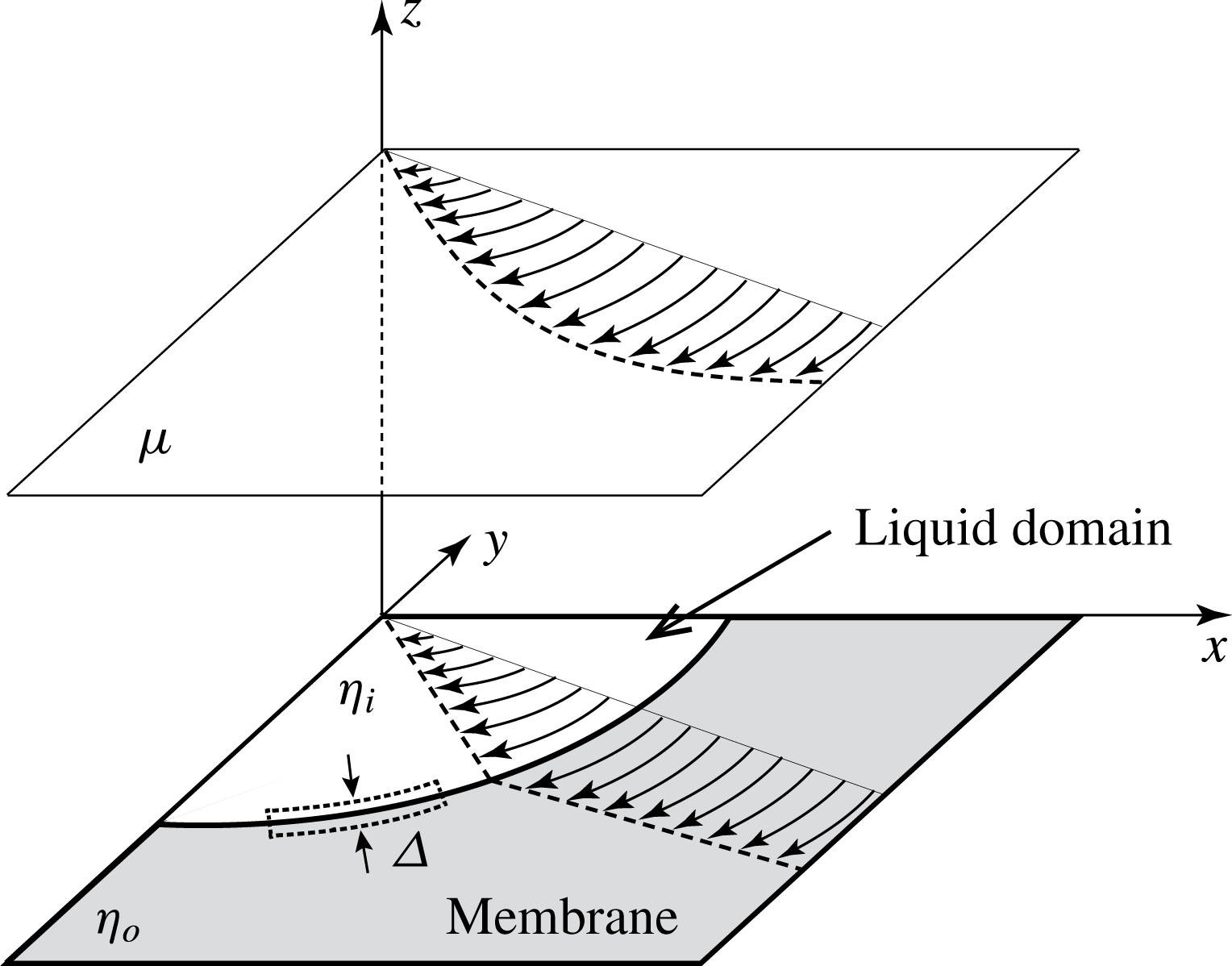
Let us consider the momentum flux passing through a 2-D slender region along the domain perimeter shown in figure 2; we write
 $\unicode[STIX]{x1D6E5}$
for its width in the direction vertical to the perimeter. As
 $\unicode[STIX]{x1D6E5}$
approaches zero, the forces exerted by the ambient 3-D fluids become negligible and mechanical balance is reached between the forces exerted by the domain interior and exterior in the membrane. Thus, the tangential stress of the 2-D fluid should be continuous across the perimeter, which is represented by
 $$\begin{eqnarray}\displaystyle \lim _{r\rightarrow a+}\unicode[STIX]{x1D70F}_{r\unicode[STIX]{x1D703}}(r,\unicode[STIX]{x1D703})=\lim _{r\rightarrow a-}\unicode[STIX]{x1D70F}_{r\unicode[STIX]{x1D703}}(r,\unicode[STIX]{x1D703}). & & \displaystyle\end{eqnarray}$$
Here,
 $\unicode[STIX]{x1D70F}$
denotes the stress tensor associated with
 $\boldsymbol{v}$
, and the limit
 $r\rightarrow a\pm$
indicates that
 $r$
approaches
 $a$
with
 $r-a$
being kept positive (negative). If
 $\unicode[STIX]{x1D702}_{i}$
equals
 $\unicode[STIX]{x1D702}_{o}$
, we can do without (2.6), which is satisfied whenever (2.5) holds and
 $\boldsymbol{V}$
is smooth. Otherwise, we should consider (2.6), which makes the velocity gradient of the 2-D fluid discontinuous across the perimeter as shown in figure 2. This point is overlooked in Fujitani (Reference Fujitani2011) and Rao & Das (Reference Rao and Das2015).
A region of
 $x>0$
,
 $y<0$
and
 $z\geqslant 0$
of figure 1 is drawn. The curved arrows in the membrane represent velocity fields of
 $\boldsymbol{v}-\boldsymbol{U}$
. Its velocity gradient should be discontinuous across the domain perimeter when
 $\unicode[STIX]{x1D702}_{i}$
is not equal to
 $\unicode[STIX]{x1D702}_{o}$
. The curved arrows in a cross-section parallel to the membrane represent
 $\boldsymbol{V}-\boldsymbol{U}$
, which is smooth in the 3-D fluid. A slender region is drawn with the dotted closed curve along the domain perimeter in the membrane. We write
 $\unicode[STIX]{x1D6E5}$
for the size in the direction vertical to the perimeter.
3 Previous results
We introduce the Fourier transforms of the fields with respect to
 $\unicode[STIX]{x1D703}$
, e.g.
 $$\begin{eqnarray}\displaystyle \tilde{V}_{zm}(r,z)\equiv \frac{1}{2\unicode[STIX]{x03C0}}\int _{0}^{2\unicode[STIX]{x03C0}}\,\text{d}\unicode[STIX]{x1D703}V_{z}(r,\unicode[STIX]{x1D703},z)\text{e}^{-\text{i}m\unicode[STIX]{x1D703}}, & & \displaystyle\end{eqnarray}$$
with
 $m=0,\pm 1,\pm 2,\ldots \,$
, and the Hankel transforms with respect to
 $r$
, e.g.
 $$\begin{eqnarray}\displaystyle \hat{V}_{zm}(\unicode[STIX]{x1D701},z)\equiv \int _{0}^{\infty }\,\text{d}r\,r\text{J}_{m}(\unicode[STIX]{x1D701}r)\tilde{V}_{zm}(r,z), & & \displaystyle\end{eqnarray}$$
where
 $\text{J}_{m}$
is the Bessel function of the first kind. Because of the symmetry, only the Fourier transforms with
 $m=\pm 1$
do not vanish. In each field, the transforms of
 $m=\pm 1$
are related to each other. Thus, we have only to consider the Fourier transforms with
 $m=1$
. As shown in appendix A, we rewrite (2.1) in Hankel transforms and solve the resultant equations for
 $m=1$
with two functions of
 $\unicode[STIX]{x1D701}$
being left undetermined. We can delete one of them with the aid of (2.5) and the second equations of (2.1) and (2.2), and thus have only to consider one undetermined function of
 $\unicode[STIX]{x1D701}$
. We introduce
 $$\begin{eqnarray}\displaystyle R\equiv \frac{r}{a}\quad \text{and}\quad \unicode[STIX]{x1D708}_{o}\equiv \frac{\unicode[STIX]{x1D702}_{o}}{2\unicode[STIX]{x1D707}a}, & & \displaystyle\end{eqnarray}$$
where
 $\unicode[STIX]{x1D708}_{o}$
is sometimes referred to as the Boussinesq number. We use (2.5) to express
 $\boldsymbol{v}$
in terms of the undetermined function. Thus, equation (2.4) yields
 $$\begin{eqnarray}\displaystyle 2\unicode[STIX]{x1D707}a^{2}U=\int _{0}^{\infty }\,\text{d}\unicode[STIX]{x1D701}\frac{\text{J}_{1}(\unicode[STIX]{x1D701})A(\unicode[STIX]{x1D701})}{\unicode[STIX]{x1D701}(1+\unicode[STIX]{x1D708}_{o}\unicode[STIX]{x1D701})}, & & \displaystyle\end{eqnarray}$$
where
 $A$
is the undetermined function. Utilizing that the left-hand side of (2.2) is irrotational and calculating
 $\boldsymbol{F}$
in terms of
 $\boldsymbol{V}$
, we obtain
 $$\begin{eqnarray}\displaystyle & \displaystyle 0=\int _{0}^{\infty }\,\text{d}\unicode[STIX]{x1D701}\,\unicode[STIX]{x1D701}^{2}\text{J}_{1}(\unicode[STIX]{x1D701}R)A(\unicode[STIX]{x1D701})\quad \text{for}~1<R\quad \text{and} & \displaystyle\end{eqnarray}$$
 $$\begin{eqnarray}\displaystyle & \displaystyle 0=\int _{0}^{\infty }\,\text{d}\unicode[STIX]{x1D701}\,\unicode[STIX]{x1D701}^{2}\text{J}_{1}(\unicode[STIX]{x1D701}R)A(\unicode[STIX]{x1D701})\left(1-\frac{\unicode[STIX]{x1D705}}{1+\unicode[STIX]{x1D708}_{o}\unicode[STIX]{x1D701}}\right)\quad \text{for}~0\leqslant R<1. & \displaystyle\end{eqnarray}$$
See appendix A for the details.
Let us define
 $q(R)$
as the integral of (3.5) for
 $R\geqslant 0$
. In Fujitani (Reference Fujitani2013a
), it was shown that the general form of the solution
 $q(R)$
is written as
 $$\begin{eqnarray}\displaystyle q(R)=q_{1}(R)+c_{1}\unicode[STIX]{x1D6FF}(R-1)+c_{2}\frac{\text{d}}{\text{d}R}\unicode[STIX]{x1D6FF}(R-1), & & \displaystyle\end{eqnarray}$$
where
 $q_{1}(R)$
is a finite function vanishing for
 $R>1$
, and
 $c_{1}$
and
 $c_{2}$
are constants independent of
 $R$
. The third term on the right-hand side above is missed in Fujitani (Reference Fujitani2011). Without this term, we can satisfy all the conditions other than (2.6), but the resultant solution is incorrect unless
 $\unicode[STIX]{x1D702}_{i}$
equals
 $\unicode[STIX]{x1D702}_{o}$
. The derivative of the delta function makes
 $\unicode[STIX]{x1D70F}_{r\unicode[STIX]{x1D703}}$
have a term proportional to the product of
 $\unicode[STIX]{x1D702}$
and a function discontinuous across
 $R=1$
, as mentioned at the end of appendix A. Thus, we can always determine
 $c_{2}$
so that the stress is continuous across the domain perimeter. As discussed at the end of Fujitani (Reference Fujitani2013a
, § 3.2), higher derivatives make
 $\boldsymbol{v}$
more singular and thus are unnecessary in (3.7). The second term on the right-hand side of (3.7) gives a point source, while the third term gives a dipole source, which is analogous to the single-layer and double-layer potentials in the boundary integral, respectively (Pozrikidis Reference Pozrikidis1992). The Hankel transformation of (3.7) involves the integral of
 $Rq_{1}(R)\text{J}_{1}(\unicode[STIX]{x1D701}R)$
over
 $0<R<1$
. Rewriting this integral with the aid of (3.6), we obtain
 $$\begin{eqnarray}\displaystyle \unicode[STIX]{x1D701}A(\unicode[STIX]{x1D701}) & = & \displaystyle c_{1}\text{J}_{1}(\unicode[STIX]{x1D701})-c_{2}\unicode[STIX]{x1D701}\text{J}_{0}(\unicode[STIX]{x1D701})+\unicode[STIX]{x1D705}\int _{0}^{\infty }\,\text{d}\unicode[STIX]{x1D709}\frac{\unicode[STIX]{x1D709}^{2}A(\unicode[STIX]{x1D709})}{1+\unicode[STIX]{x1D708}_{o}\unicode[STIX]{x1D709}}\int _{0}^{1}\,\text{d}R\,R\text{J}_{1}(\unicode[STIX]{x1D701}R)\text{J}_{1}(\unicode[STIX]{x1D709}R)\end{eqnarray}$$
 $$\begin{eqnarray}\displaystyle & = & \displaystyle c_{1}\text{J}_{1}(\unicode[STIX]{x1D701})-c_{2}\unicode[STIX]{x1D701}\text{J}_{0}(\unicode[STIX]{x1D701})+\unicode[STIX]{x1D705}\unicode[STIX]{x1D701}\int _{0}^{\infty }\,\text{d}\unicode[STIX]{x1D709}\,K(\unicode[STIX]{x1D701},\unicode[STIX]{x1D709})A(\unicode[STIX]{x1D709}),\end{eqnarray}$$
where the kernel is defined as
 $$\begin{eqnarray}\displaystyle K(\unicode[STIX]{x1D701},\unicode[STIX]{x1D709})\equiv \frac{\unicode[STIX]{x1D709}^{2}}{(1+\unicode[STIX]{x1D708}_{o}\unicode[STIX]{x1D709})\unicode[STIX]{x1D701}}\times \frac{\unicode[STIX]{x1D709}\text{J}_{0}(\unicode[STIX]{x1D709})\text{J}_{1}(\unicode[STIX]{x1D701})-\unicode[STIX]{x1D701}\text{J}_{0}(\unicode[STIX]{x1D701})\text{J}_{1}(\unicode[STIX]{x1D709})}{\unicode[STIX]{x1D701}^{2}-\unicode[STIX]{x1D709}^{2}}. & & \displaystyle\end{eqnarray}$$
Equation (3.8) is essentially derived in Fujitani (Reference Fujitani2013a
, §3.2) although not shown explicitly because the discussion is mainly focused on the order of
 $\unicode[STIX]{x1D705}$
there. The constants
 $c_{1}$
and
 $c_{2}$
can be determined with the aid of (2.6) and (3.4). Another kernel,
 $M$
, is used in Fujitani (Reference Fujitani2013a
); its definition and relation to
 $K$
are given by
 $$\begin{eqnarray}\displaystyle M(\unicode[STIX]{x1D701},\unicode[STIX]{x1D709}) & \equiv & \displaystyle \frac{\unicode[STIX]{x1D709}}{1+\unicode[STIX]{x1D708}_{o}\unicode[STIX]{x1D709}}\times \frac{\unicode[STIX]{x1D701}\text{J}_{0}(\unicode[STIX]{x1D709})\text{J}_{1}(\unicode[STIX]{x1D701})-\unicode[STIX]{x1D709}\text{J}_{0}(\unicode[STIX]{x1D701})\text{J}_{1}(\unicode[STIX]{x1D709})}{\unicode[STIX]{x1D701}^{2}-\unicode[STIX]{x1D709}^{2}}\end{eqnarray}$$
 $$\begin{eqnarray}\displaystyle & = & \displaystyle K(\unicode[STIX]{x1D701},\unicode[STIX]{x1D709})+\frac{\unicode[STIX]{x1D709}\text{J}_{0}(\unicode[STIX]{x1D709})\text{J}_{1}(\unicode[STIX]{x1D701})}{(1+\unicode[STIX]{x1D708}_{o}\unicode[STIX]{x1D709})\unicode[STIX]{x1D701}}.\end{eqnarray}$$
As shown in appendix A, the drag coefficient is given by
 $$\begin{eqnarray}\displaystyle \unicode[STIX]{x1D6FE}=\lim _{R\rightarrow 1+}\lim _{Z\rightarrow 0+}\left[\frac{\unicode[STIX]{x03C0}}{aU}\int _{0}^{\infty }\,\text{d}\unicode[STIX]{x1D701}\,\unicode[STIX]{x1D701}J_{2}(\unicode[STIX]{x1D701}R)A(\unicode[STIX]{x1D701})\text{e}^{-\unicode[STIX]{x1D701}Z}\right], & & \displaystyle\end{eqnarray}$$
where
 $Z\equiv z/a$
.
When
 $\unicode[STIX]{x1D705}$
vanishes, we have
 $c_{2}=0$
and find
 $$\begin{eqnarray}\displaystyle A(\unicode[STIX]{x1D701})=\frac{2\unicode[STIX]{x1D707}a^{2}U}{Y_{0}(\unicode[STIX]{x1D708}_{o})}\frac{\text{J}_{1}(\unicode[STIX]{x1D701})}{\unicode[STIX]{x1D701}}\quad \text{for}~\unicode[STIX]{x1D705}=0, & & \displaystyle\end{eqnarray}$$
where
 $Y_{0}$
is defined as
 $$\begin{eqnarray}\displaystyle Y_{0}(\unicode[STIX]{x1D708}_{o})=\int _{0}^{\infty }\,\text{d}\unicode[STIX]{x1D701}\frac{\text{J}_{1}^{2}(\unicode[STIX]{x1D701})}{\unicode[STIX]{x1D701}^{2}(1+\unicode[STIX]{x1D708}_{o}\unicode[STIX]{x1D701})}. & & \displaystyle\end{eqnarray}$$
Equation (3.14) is substituted into (3.13) to yield the previous result of Koker (Reference De Koker1996). Writing
 $\unicode[STIX]{x1D6FE}_{\unicode[STIX]{x1D705}=0}$
for his result of the drag coefficient, we have
 $$\begin{eqnarray}\displaystyle \unicode[STIX]{x1D6FE}_{\unicode[STIX]{x1D705}=0}=\frac{2\unicode[STIX]{x03C0}\unicode[STIX]{x1D707}a}{Y_{0}(\unicode[STIX]{x1D708}_{o})}, & & \displaystyle\end{eqnarray}$$
For a rigid disk, equation (2.4) is replaced by
 $\boldsymbol{v}=\boldsymbol{U}$
for
 $r\leqslant a$
, and (2.6) is not required, as was discussed in Saffman (Reference Saffman1976) and Hughes et al. (Reference Hughes, Pailthorpe and White1981). Equation (3.50) in the latter reference can be rewritten as a set of simultaneous equations with respect to
 $\unicode[STIX]{x1D714}_{0},\unicode[STIX]{x1D714}_{1},\ldots \,$
, i.e.
 $$\begin{eqnarray}\displaystyle \unicode[STIX]{x1D6FF}_{l,0}=\mathop{\sum }_{m=0}^{\infty }\unicode[STIX]{x1D714}_{m}\left[\int _{0}^{\infty }\,\text{d}u\frac{\text{j}_{2l}(u)\text{j}_{2m}(u)}{u+\unicode[STIX]{x1D708}_{o}^{-1}}\right]\quad \text{for}~l=0,1,2,\ldots . & & \displaystyle\end{eqnarray}$$
Here,
 $\unicode[STIX]{x1D6FF}_{i,j}$
denotes Kronecker’s delta and
 $\text{j}_{0}(u),\text{j}_{2}(u),\ldots$
denote the spherical Bessel functions. According to Hughes et al. (Reference Hughes, Pailthorpe and White1981),
 $\unicode[STIX]{x1D714}_{0}$
is related to the drag coefficient of a rigid disk, for which we write
 $\unicode[STIX]{x1D6FE}_{disk}$
, as
 $$\begin{eqnarray}\displaystyle \unicode[STIX]{x1D6FE}_{disk}=4\unicode[STIX]{x03C0}\unicode[STIX]{x1D702}_{o}\unicode[STIX]{x1D714}_{0}. & & \displaystyle\end{eqnarray}$$
The dimensionless quantity
 $\unicode[STIX]{x1D714}_{0}=\unicode[STIX]{x1D6FE}_{disk}/4\unicode[STIX]{x03C0}\unicode[STIX]{x1D702}_{o}$
is determined only by
 $\unicode[STIX]{x1D708}_{o}$
. According to Saffman & Delbrück (Reference Saffman and Delbrück1975), Saffman (Reference Saffman1976), Hughes et al. (Reference Hughes, Pailthorpe and White1981), we have
 $$\begin{eqnarray}\displaystyle \frac{4\unicode[STIX]{x03C0}\unicode[STIX]{x1D702}_{o}}{\unicode[STIX]{x1D6FE}_{disk}}\approx \left\{\begin{array}{@{}ll@{}}\ln (2\unicode[STIX]{x1D708}_{o})-0.577\approx \ln (1.12\unicode[STIX]{x1D708}_{o})\quad & \text{for}~\unicode[STIX]{x1D708}_{o}\gg 1,\\ \unicode[STIX]{x03C0}\unicode[STIX]{x1D708}_{o}/2\approx \unicode[STIX]{x1D708}_{o}/0.637\quad & \text{for}~\unicode[STIX]{x1D708}_{o}\ll 1.\end{array}\right. & & \displaystyle\end{eqnarray}$$
We also find the quotient of (3.16) divided by
 $4\unicode[STIX]{x03C0}\unicode[STIX]{x1D702}_{o}$
to be a dimensionless quantity determined only by
 $\unicode[STIX]{x1D708}_{o}$
because of
 $$\begin{eqnarray}\displaystyle \frac{\unicode[STIX]{x1D6FE}_{\unicode[STIX]{x1D705}=0}}{4\unicode[STIX]{x03C0}\unicode[STIX]{x1D702}_{o}}=\frac{1}{4\unicode[STIX]{x1D708}_{o}Y_{0}(\unicode[STIX]{x1D708}_{o})}. & & \displaystyle\end{eqnarray}$$
As discussed in Koker (Reference De Koker1996) and Fujitani (Reference Fujitani2011), we have
 $$\begin{eqnarray}\displaystyle \frac{4\unicode[STIX]{x03C0}\unicode[STIX]{x1D702}_{o}}{\unicode[STIX]{x1D6FE}_{\unicode[STIX]{x1D705}=0}}\approx \left\{\begin{array}{@{}ll@{}}\ln (1.44\unicode[STIX]{x1D708}_{o})\quad & \text{for}~\unicode[STIX]{x1D708}_{o}\gg 1,\\ 16\unicode[STIX]{x1D708}_{o}/3\unicode[STIX]{x03C0}\approx \unicode[STIX]{x1D708}_{o}/0.589\quad & \text{for}~\unicode[STIX]{x1D708}_{o}\ll 1.\end{array}\right. & & \displaystyle\end{eqnarray}$$
The ratio of
 $\unicode[STIX]{x1D6FE}_{disk}$
to
 $\unicode[STIX]{x1D6FE}_{\unicode[STIX]{x1D705}=0}$
also depends only on
 $\unicode[STIX]{x1D708}_{o}$
. We write
 $\tilde{\unicode[STIX]{x1D6FE}}_{disk}(\unicode[STIX]{x1D708}_{o})$
for the ratio, i.e.
 $$\begin{eqnarray}\tilde{\unicode[STIX]{x1D6FE}}_{disk}(\unicode[STIX]{x1D708}_{o})=\frac{\unicode[STIX]{x1D6FE}_{disk}}{\unicode[STIX]{x1D6FE}_{\unicode[STIX]{x1D705}=0}}.\end{eqnarray}$$
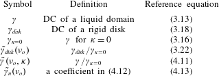
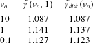
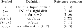
Some definitions are summarized in table 1.
Definitions of
 $\unicode[STIX]{x1D6FE}$
and the related quantities. Here, DC means the drag coefficient.
Typical values of
 $\unicode[STIX]{x1D707}$
and
 $\unicode[STIX]{x1D702}_{o}$
are respectively
 $1~\text{g}~(\text{m}\text{s})^{-1}$
and
 $10^{-7}~\text{g}~\text{s}^{-1}$
(Merkel, Sackmann & Evans Reference Merkel, Sackmann and Evans1989; Smeulders, Blom & Mellema Reference Smeulders, Blom and Mellema1990). We can calculate
 $\unicode[STIX]{x1D6FE}_{disk}(\unicode[STIX]{x1D708}_{o})/4\unicode[STIX]{x03C0}\unicode[STIX]{x1D702}_{o}$
by truncating the sum in (3.17) up to
 $m=20$
; the absolute value of the change in the result obtained when we use the sum up to
 $m=21$
is much smaller than
 $10^{-3}$
for each of the values
 $\unicode[STIX]{x1D708}_{o}$
considered. The previous results for
 $\unicode[STIX]{x1D708}_{o}=10,1$
and
 $0.1$
are summarized in table 2.
4 Results
4.1 Analytical results
Considering (3.14), it is convenient to introduce
 $$\begin{eqnarray}\displaystyle A(\unicode[STIX]{x1D701})=\frac{2\unicode[STIX]{x1D707}a^{2}U}{Y_{0}(\unicode[STIX]{x1D708}_{o})}\tilde{A}(\unicode[STIX]{x1D701}). & & \displaystyle\end{eqnarray}$$
We expand
 $\tilde{A}$
with respect to
 $\unicode[STIX]{x1D705}$
as
 $$\begin{eqnarray}\displaystyle \tilde{A}(\unicode[STIX]{x1D701})=\mathop{\sum }_{n=0}^{\infty }\unicode[STIX]{x1D705}^{n}\tilde{A}_{n}(\unicode[STIX]{x1D701}), & & \displaystyle\end{eqnarray}$$
where
 $$\begin{eqnarray}\displaystyle \tilde{A}_{0}(\unicode[STIX]{x1D701})=\frac{\text{J}_{1}(\unicode[STIX]{x1D701})}{\unicode[STIX]{x1D701}}. & & \displaystyle\end{eqnarray}$$
Let us define an operator
 $\hat{M}$
as
 $$\begin{eqnarray}\displaystyle [\hat{M}f](\unicode[STIX]{x1D701})\equiv \int _{0}^{\infty }\,\text{d}\unicode[STIX]{x1D709}M(\unicode[STIX]{x1D701},\unicode[STIX]{x1D709})f(\unicode[STIX]{x1D709}), & & \displaystyle\end{eqnarray}$$
where
 $f$
is a function. From (3.9), as shown in appendix B, we derive
 $$\begin{eqnarray}\displaystyle \tilde{A}_{n}(\unicode[STIX]{x1D701})=\unicode[STIX]{x1D6FC}_{n}\frac{\text{J}_{1}(\unicode[STIX]{x1D701})}{\unicode[STIX]{x1D701}}+\unicode[STIX]{x1D6FD}_{n}\text{J}_{0}(\unicode[STIX]{x1D701})+[\hat{M}\tilde{A}_{n-1}](\unicode[STIX]{x1D701})\quad \text{for}~n=0,1,2,\ldots . & & \displaystyle\end{eqnarray}$$
Here, we stipulate
 $\unicode[STIX]{x1D6FC}_{0}=1$
,
 $\unicode[STIX]{x1D6FD}_{0}=0$
and
 $\tilde{A}_{-1}=0$
, which give (4.3). The constants
 $\unicode[STIX]{x1D6FC}_{n}$
and
 $\unicode[STIX]{x1D6FD}_{n}$
for
 $n\geqslant 1$
depend only on
 $\unicode[STIX]{x1D708}_{o}$
, as shown below.
Previous results.
 $\dagger$
Values calculated by using typical values of
 $\unicode[STIX]{x1D707}$
and
 $\unicode[STIX]{x1D702}_{o}$
mentioned in the text.

Substituting (4.1), (4.2) and (4.5) into (3.4) yields
 $$\begin{eqnarray}\displaystyle \unicode[STIX]{x1D6FC}_{n}=-\frac{1}{Y_{0}}(\unicode[STIX]{x1D6FD}_{n}X+\hat{L}\hat{M}\tilde{A}_{n-1})\quad \text{for}~n=1,2,\ldots . & & \displaystyle\end{eqnarray}$$
As shown in appendix B, substituting (4.1), (4.2) and (4.5) into (2.6) yields
 $$\begin{eqnarray}\displaystyle \unicode[STIX]{x1D6FD}_{n}=\unicode[STIX]{x1D708}_{o}(\unicode[STIX]{x1D6FC}_{n-1}\hat{N}\tilde{A}_{0}+\unicode[STIX]{x1D6FD}_{n-1}{\mathcal{G}}+\hat{N}\hat{M}\tilde{A}_{n-2})\quad \text{for}~n=1,2,\ldots . & & \displaystyle\end{eqnarray}$$
Here, we use
 $$\begin{eqnarray}X\equiv \int _{0}^{\infty }\,\text{d}\unicode[STIX]{x1D701}\frac{\text{J}_{1}(\unicode[STIX]{x1D701})\text{J}_{0}(\unicode[STIX]{x1D701})}{\unicode[STIX]{x1D701}(1+\unicode[STIX]{x1D708}_{o}\unicode[STIX]{x1D701})},\quad {\mathcal{G}}\equiv \lim _{R\rightarrow 1+}\int _{0}^{\infty }\,\text{d}\unicode[STIX]{x1D701}\frac{\unicode[STIX]{x1D701}\text{J}_{2}^{\prime }(\unicode[STIX]{x1D701}R)\text{J}_{0}(\unicode[STIX]{x1D701})}{1+\unicode[STIX]{x1D708}_{o}\unicode[STIX]{x1D701}},\end{eqnarray}$$
 $$\begin{eqnarray}\hat{N}f\equiv \int _{0}^{\infty }\,\text{d}\unicode[STIX]{x1D701}\frac{\unicode[STIX]{x1D701}\text{J}_{2}^{\prime }(\unicode[STIX]{x1D701})}{1+\unicode[STIX]{x1D708}_{o}\unicode[STIX]{x1D701}}f(\unicode[STIX]{x1D701}),\quad \text{and}\quad \hat{L}f\equiv \int _{0}^{\infty }\,\text{d}\unicode[STIX]{x1D701}\frac{\text{J}_{1}(\unicode[STIX]{x1D701})}{\unicode[STIX]{x1D701}(1+\unicode[STIX]{x1D708}_{o}\unicode[STIX]{x1D701})}f(\unicode[STIX]{x1D701}),\end{eqnarray}$$
where
 $f$
is a function and
 $J_{2}^{\prime }(\unicode[STIX]{x1D701})$
implies
 $$\begin{eqnarray}J_{2}^{\prime }(\unicode[STIX]{x1D701})\equiv \frac{\text{d}J_{2}(\unicode[STIX]{x1D701})}{\text{d}\unicode[STIX]{x1D701}}=\text{J}_{1}(\unicode[STIX]{x1D701})-\frac{2J_{2}(\unicode[STIX]{x1D701})}{\unicode[STIX]{x1D701}}.\end{eqnarray}$$
We have
 $Y_{0}=\hat{L}\tilde{A}_{0}$
. The integral in the second equation of (4.8) is a function of
 $R$
and is discontinuous at
 $R=1$
because the integrand does not approach zero rapidly as
 $\unicode[STIX]{x1D701}$
increases.
In general, the drag coefficient
 $\unicode[STIX]{x1D6FE}$
depends on
 $a$
,
 $\unicode[STIX]{x1D707}$
,
 $\unicode[STIX]{x1D702}_{o}$
and
 $\unicode[STIX]{x1D702}_{i}$
. In (3.16),
 $\unicode[STIX]{x1D6FE}_{\unicode[STIX]{x1D705}=0}$
depends on
 $a$
,
 $\unicode[STIX]{x1D707}$
and
 $\unicode[STIX]{x1D702}_{o}$
. As shown below, the ratio
 $\unicode[STIX]{x1D6FE}/\unicode[STIX]{x1D6FE}_{\unicode[STIX]{x1D705}=0}$
depends only on
 $\unicode[STIX]{x1D708}_{o}$
and
 $\unicode[STIX]{x1D705}$
. Substituting (4.1), (4.2) and (4.5) into (3.13), we obtain
 $$\begin{eqnarray}\displaystyle \unicode[STIX]{x1D6FE}=\unicode[STIX]{x1D6FE}_{\unicode[STIX]{x1D705}=0}\tilde{\unicode[STIX]{x1D6FE}}(\unicode[STIX]{x1D708}_{o},\unicode[STIX]{x1D705}), & & \displaystyle\end{eqnarray}$$
where
 $\tilde{\unicode[STIX]{x1D6FE}}(\unicode[STIX]{x1D708}_{o},\unicode[STIX]{x1D705})$
is defined as
 $$\begin{eqnarray}\displaystyle \tilde{\unicode[STIX]{x1D6FE}}(\unicode[STIX]{x1D708}_{o},\unicode[STIX]{x1D705})=\mathop{\sum }_{n=0}^{\infty }\tilde{\unicode[STIX]{x1D6FE}}_{n}(\unicode[STIX]{x1D708}_{o})\unicode[STIX]{x1D705}^{n}, & & \displaystyle\end{eqnarray}$$
with
 $\tilde{\unicode[STIX]{x1D6FE}}_{n}$
being given by
 $$\begin{eqnarray}\displaystyle \tilde{\unicode[STIX]{x1D6FE}}_{n}(\unicode[STIX]{x1D708}_{o})=\unicode[STIX]{x1D6FC}_{n}+2\unicode[STIX]{x1D6FD}_{n}+\lim _{R\rightarrow 1+}\lim _{Z\rightarrow 0+}\left[\int _{0}^{\infty }\,\text{d}\unicode[STIX]{x1D701}\,\unicode[STIX]{x1D701}J_{2}(\unicode[STIX]{x1D701}R)[\hat{M}\tilde{A}_{n-1}](\unicode[STIX]{x1D701})\text{e}^{-\unicode[STIX]{x1D701}Z}\right]\quad \text{for}~n=1,2,\ldots & & \displaystyle \nonumber\\ \displaystyle & & \displaystyle\end{eqnarray}$$
and
 $\tilde{\unicode[STIX]{x1D6FE}}_{0}(\unicode[STIX]{x1D708}_{o})=1$
. This equality implies
 $\tilde{\unicode[STIX]{x1D6FE}}(\unicode[STIX]{x1D708}_{o},0)=1$
, as it should be. The term in the brackets above in the limit of
 $Z\rightarrow 0+$
is discontinuous at
 $R=1$
.
4.2 Numerical results
In the following numerical calculations, we use the software of Wolfram Mathematica® version 10 (Wolfram Research). To obtain
 $\unicode[STIX]{x1D6FC}_{n}$
,
 $\unicode[STIX]{x1D6FD}_{n}$
and
 $\tilde{A}_{n}$
successively by using (4.5)–(4.7), we numerically calculate the integrals appearing in (3.15), (4.4), (4.8) and (4.9). When the upper bound
 $\infty$
is required to be changed to a finite value, we put it equal to
 $10^{4}$
. The integrals appear to remain unchanged even if the upper bounds are raised from
 $10^{4}$
, except for some integrals involving
 $\hat{M}\text{J}_{0}$
mentioned later. The following procedure is used in calculating
 ${\mathcal{G}}$
. In the integral of the second equation of (4.8),
 $J_{2}^{\prime }$
is rewritten as in (4.10) and the factor
 $\unicode[STIX]{x1D701}/(1+\unicode[STIX]{x1D708}_{o}\unicode[STIX]{x1D701})$
is rewritten as
 $\unicode[STIX]{x1D708}_{o}^{-1}-\unicode[STIX]{x1D708}_{o}^{-1}(1+\unicode[STIX]{x1D708}_{o}\unicode[STIX]{x1D701})^{-1}$
. The integral involving both the first term
 $\unicode[STIX]{x1D708}_{o}^{-1}$
and the term
 $\text{J}_{1}(\unicode[STIX]{x1D701}R)$
is discontinuous and its value at
 $R\rightarrow 1+$
is
 $\unicode[STIX]{x1D708}_{o}^{-1}$
, as shown in Fujitani (Reference Fujitani2013a
, Appendix B). The rest of the integral is continuous at
 $R=1$
, and thus is easy to evaluate numerically.
We define
 $\tilde{B}_{n}(\unicode[STIX]{x1D701})$
as
 $\tilde{A}_{n}(\unicode[STIX]{x1D701})-\unicode[STIX]{x1D6FD}_{n}\text{J}_{0}(\unicode[STIX]{x1D701})$
. Equations (4.6) and (4.7) have
 $\hat{L}\hat{M}\tilde{A}_{n-1}$
and
 $\hat{N}\hat{M}\tilde{A}_{n-2}$
, which are integrals of functions taking the form of
 $\hat{M}\tilde{A}_{m}\equiv \hat{M}\tilde{B}_{m}+\unicode[STIX]{x1D6FD}_{m}\hat{M}\text{J}_{0}$
. The first term
 $\hat{M}\tilde{B}_{m}$
can be rewritten as
 $$\begin{eqnarray}\displaystyle \unicode[STIX]{x1D6FC}_{m}\hat{M}\tilde{A}_{0}+\unicode[STIX]{x1D6FD}_{m-1}\hat{M}\hat{M}\text{J}_{0}+\hat{M}\hat{M}\tilde{B}_{m-1} & & \displaystyle\end{eqnarray}$$
because of (4.5). Thus, some integrands contain the function
 $[\hat{M}\text{J}_{0}](\unicode[STIX]{x1D701})$
, which tends to zero more slowly as
 $\unicode[STIX]{x1D701}$
increases than the other functions appearing after the operation of
 $\hat{M}$
, as mentioned in appendix C. However, the contributions of
 $\hat{L}\hat{M}\tilde{A}_{n-1}$
and
 $\hat{N}\hat{M}\tilde{A}_{n-2}$
to
 $\unicode[STIX]{x1D6FC}_{n}$
and
 $\unicode[STIX]{x1D6FD}_{n}$
are much less than those of the other terms in (4.6) and (4.7), as far as examined extensively. Thus, we use
 $10^{4}$
as the finite upper bound required in calculating
 $\unicode[STIX]{x1D6FC}_{n}$
and
 $\unicode[STIX]{x1D6FD}_{n}$
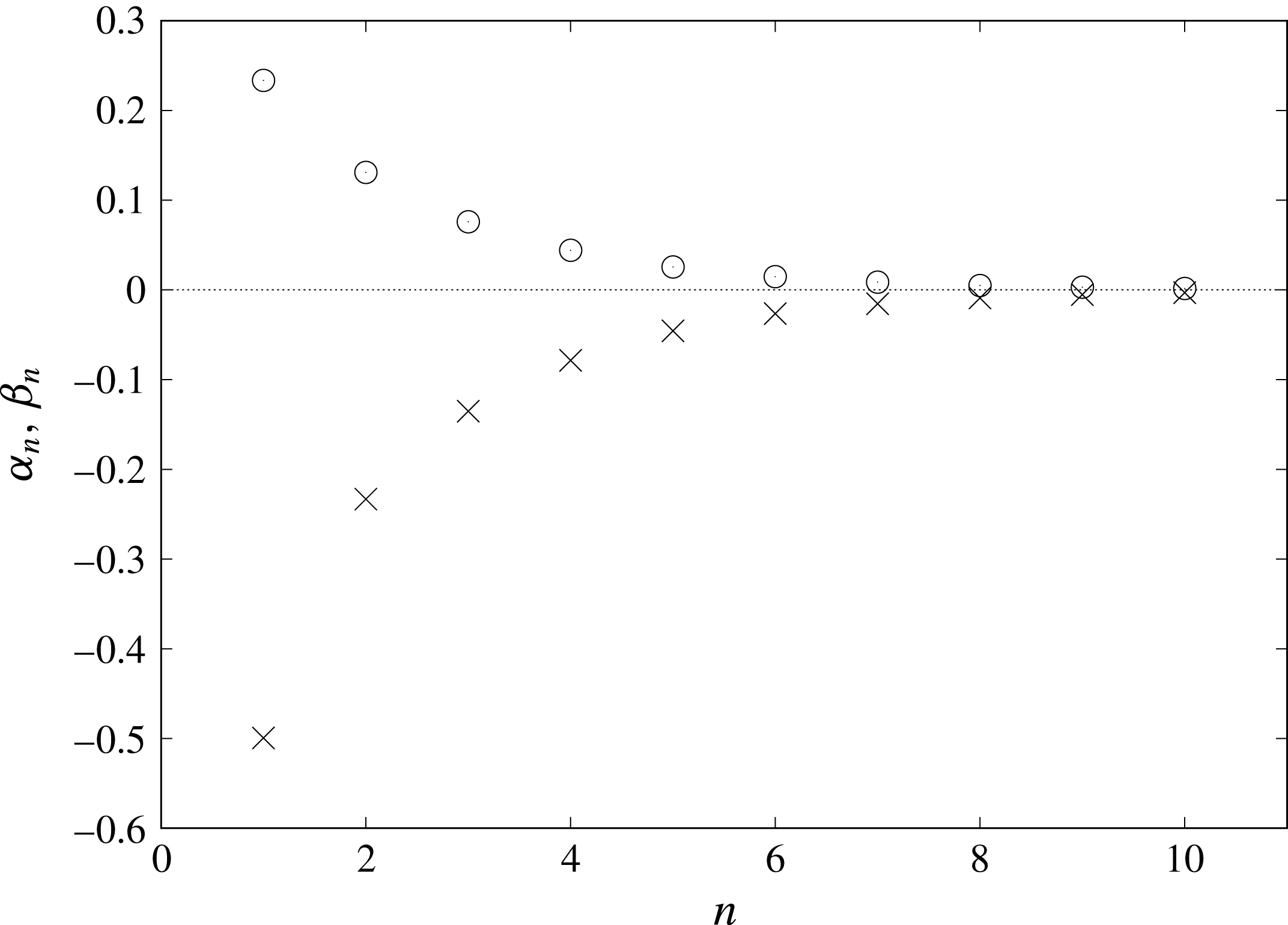
numerically. The results for
 $\unicode[STIX]{x1D708}_{o}=10$
are shown in figure 3, where
 $|\unicode[STIX]{x1D6FC}_{n}|$
and
 $\unicode[STIX]{x1D6FD}_{n}$
decrease monotonically as
 $n$
increases. They approach zero more slowly for
 $\unicode[STIX]{x1D708}_{o}=1$
and
 $\unicode[STIX]{x1D708}_{o}=0.1$
although data are not shown.
The upper bound is to be replaced by a finite value for the integral appearing explicitly in (4.13). To evaluate the integral in the limit of
 $Z\rightarrow 0+$
, we examine how the integral changes as the upper bound increases after putting
 $Z$
equal to zero. For a sufficiently large upper bound, we numerically calculate the integral for values of
 $R$
larger than and close to unity. Actually, we calculate the third term of the right-hand side of (4.13) by separating it as follows. We define the operator
 $\unicode[STIX]{x1D6E9}$
so that the third term is equal to
 $\unicode[STIX]{x1D6E9}\hat{M}\tilde{A}_{n-1}$
, which is rewritten as
 $$\begin{eqnarray}\unicode[STIX]{x1D6E9}\hat{M}\tilde{B}_{n-1}+\unicode[STIX]{x1D6FD}_{n-1}\unicode[STIX]{x1D6E9}\hat{M}\text{J}_{0}.\end{eqnarray}$$
We calculate each term above separately by using the option Global Adaptive and choose the Max Error Increases as
 $10^{4}$
in Mathematica®. The integral for
 $\unicode[STIX]{x1D6E9}\hat{M}\tilde{B}_{n-1}$
with the upper bound being
 $10^{4}$
oscillates with
 $R$
. We evaluate the integral in the limit of
 $R\rightarrow 1+$
by extrapolating the least-squares linear-regression equation, which we obtain by using the numerical results from
 $R=1.001$
to
 $1.01$
with the intervals being
 $0.0001$
. The numerical procedure for
 $\unicode[STIX]{x1D6E9}\hat{M}\text{J}_{0}$
is mentioned in appendix C. In our numerical calculations, as mentioned there, the main contribution to (4.13) usually comes from the first and second terms on the right-hand side, but the third cannot be negligible.
Numerical results of
 $\unicode[STIX]{x1D6FC}_{n}$
(crosses) and
 $\unicode[STIX]{x1D6FD}_{n}$
(circles) for
 $\unicode[STIX]{x1D708}_{o}=10$
.

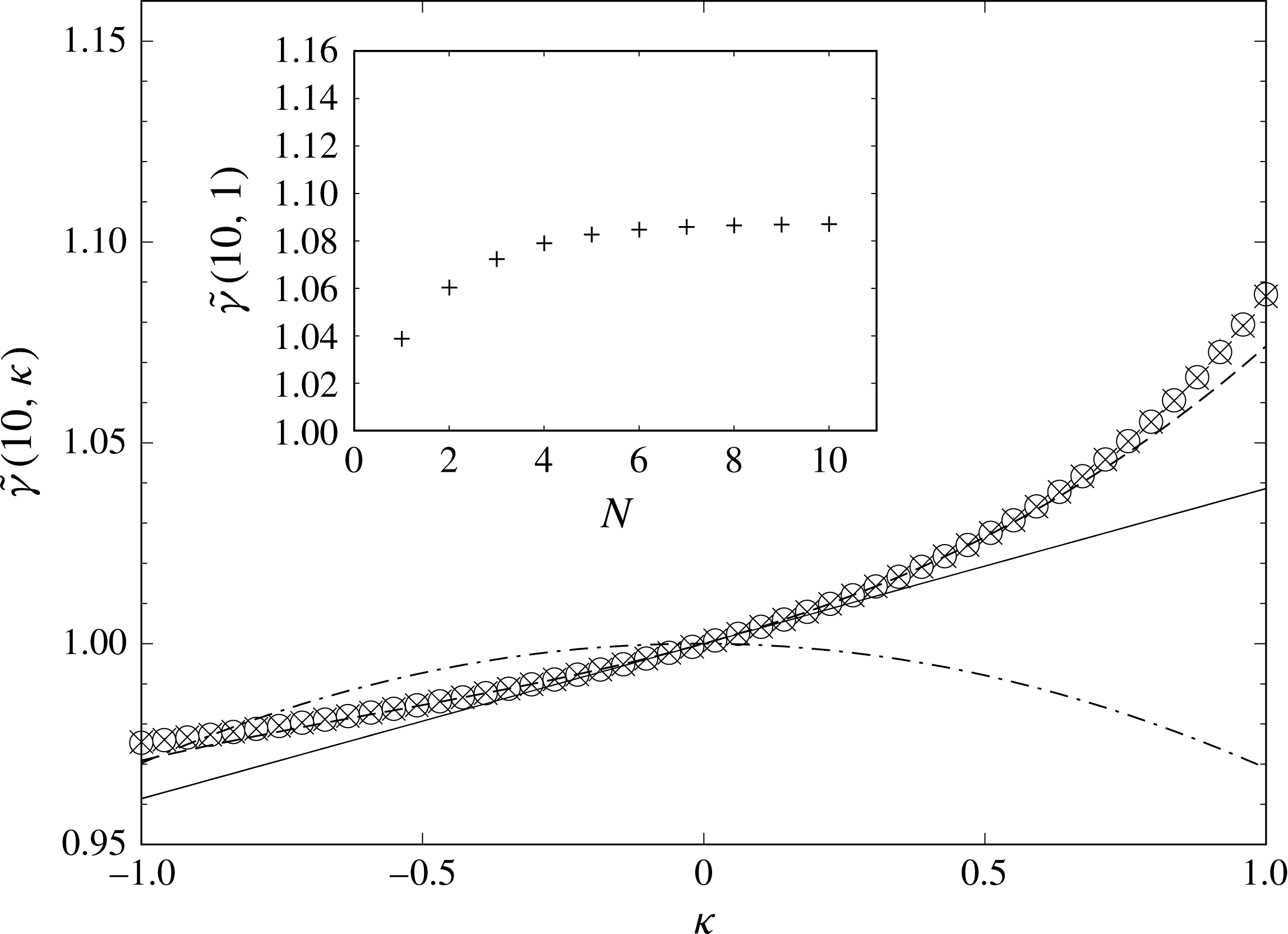
Numerical results of (4.16) for
 $\unicode[STIX]{x1D708}_{o}=10$
are shown for
 $N=1$
(solid line),
 $3$
(dotted line),
 $8$
(crosses) and
 $10$
(circles). Dashed-dotted curve represents the result calculated with
 $\unicode[STIX]{x1D6FD}_{n}$
put equal to zero for any
 $n$
. The inset shows how the numerical results at
 $\unicode[STIX]{x1D705}=1$
depend on
 $N$
.

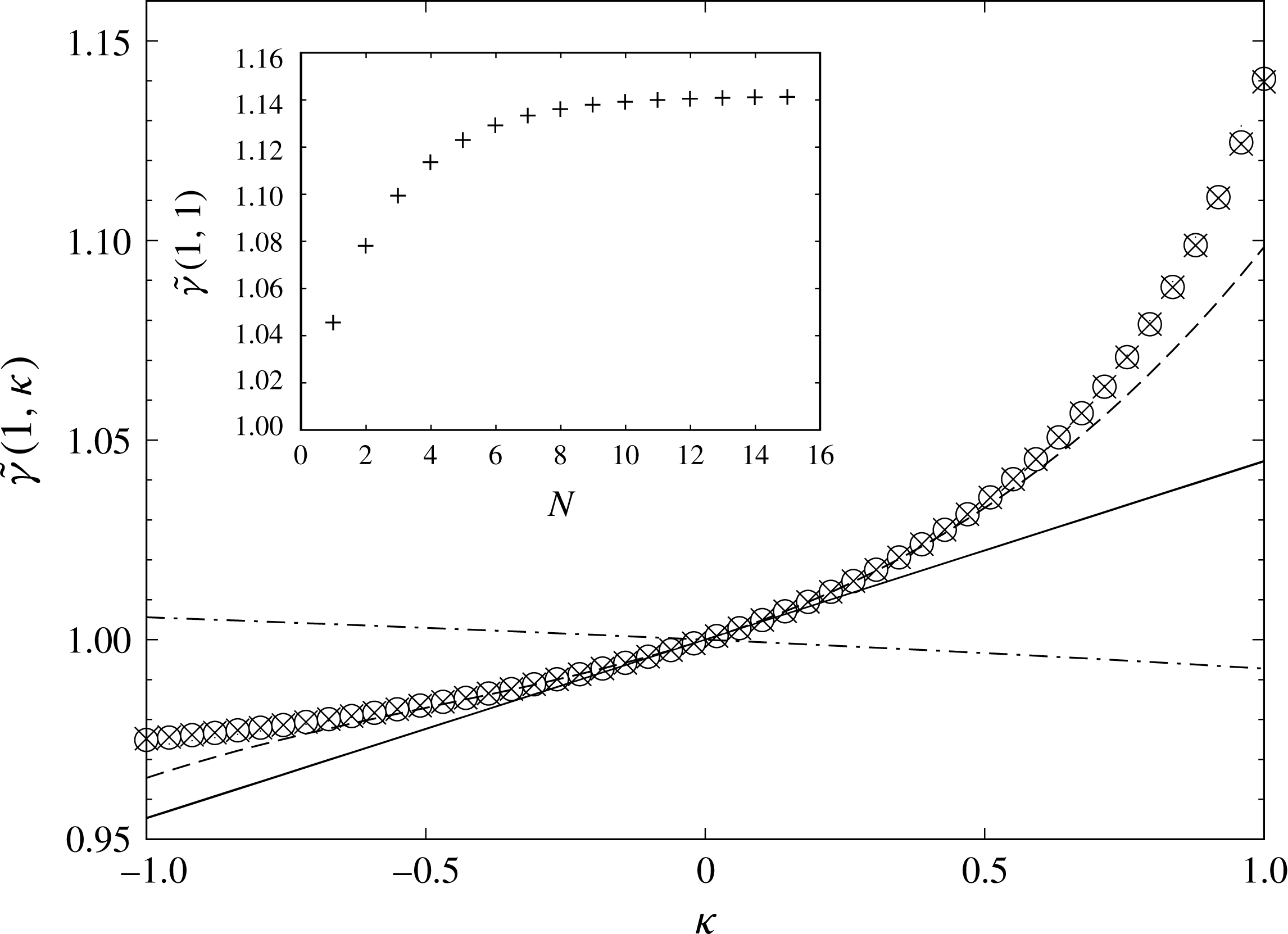
Numerical results of (4.16) for
 $\unicode[STIX]{x1D708}_{o}=1$
are shown for
 $N=1$
(solid line),
 $3$
(dotted line),
 $12$
(crosses) and
 $15$
(circles). Dashed-dotted curve represents the result calculated with
 $\unicode[STIX]{x1D6FD}_{n}$
put equal to zero for any
 $n$
. The inset shows how the numerical results at
 $\unicode[STIX]{x1D705}=1$
depend on
 $N$
.

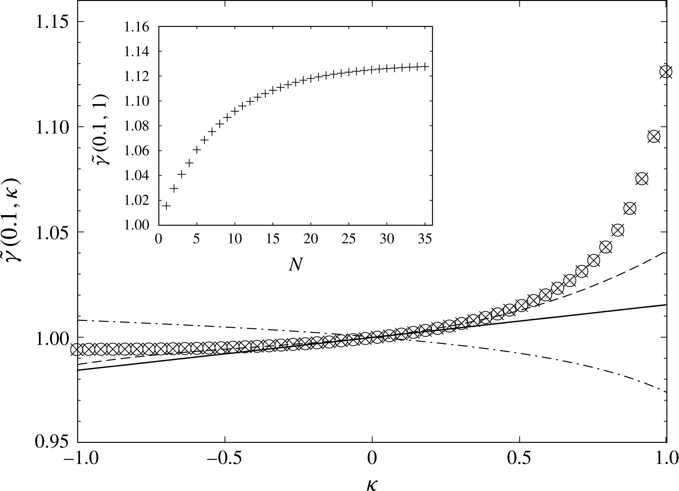
Numerical results of (4.16) for
 $\unicode[STIX]{x1D708}_{o}=0.1$
are shown for
 $N=1$
(solid line),
 $3$
(dotted line),
 $33$
(crosses) and
 $35$
(circles). Dashed-dotted curve represents the result calculated with
 $\unicode[STIX]{x1D6FD}_{n}$
put equal to zero for any
 $n$
. The inset shows how the numerical results at
 $\unicode[STIX]{x1D705}=1$
depend on
 $N$
.

For the numerical calculation of (4.12), we should truncate the series into the sum of the first
 $N$
terms as
 $$\begin{eqnarray}\displaystyle \mathop{\sum }_{n=0}^{N}\tilde{\unicode[STIX]{x1D6FE}}_{n}(\unicode[STIX]{x1D708}_{o})\unicode[STIX]{x1D705}^{n}. & & \displaystyle\end{eqnarray}$$
Our numerical results are shown for different values of
 $\unicode[STIX]{x1D708}_{o}$
in figures 4–6. The results for
 $N=1$
are also calculated in Fujitani (Reference Fujitani2013a
); the slopes of the solid lines in figures 4–6 are respectively
 $0.0385$
,
 $0.0448$
and
 $0.0156$
, which agree well with the corresponding values in the column of
 $H\rightarrow \infty$
of Fujitani (Reference Fujitani2013a
, table II). Over the region of
 $\unicode[STIX]{x1D705}$
examined in each figure, equation (4.16) approaches the curve represented by the circles as
 $N$
increases. As shown by each inset figure, the increment of (4.16) occurring at
 $\unicode[STIX]{x1D705}=1$
when
 $N$
increases by one decreases with
 $N$
. For
 $\unicode[STIX]{x1D708}_{o}=10$
, the increment is much smaller than
 $10^{-3}$
for
 $N\geqslant 9$
, and we regard (4.16) with
 $N=10$
as the value of (4.12). For
 $\unicode[STIX]{x1D708}_{o}=1$
, the increment is much smaller than
 $10^{-3}$
for
 $N\geqslant 14$
, and we regard (4.16) with
 $N=15$
as the value of (4.12). For
 $\unicode[STIX]{x1D708}_{o}=0.1$
, the increment is much smaller than
 $10^{-3}$
for
 $N\geqslant 34$
, and we regard (4.16) with
 $N=35$
as the value of (4.12). As far as examined,
 $\tilde{\unicode[STIX]{x1D6FE}}$
increases with
 $\unicode[STIX]{x1D705}$
. For each of
 $\unicode[STIX]{x1D708}_{o}=10$
and
 $1$
, the sum up to
 $N=1$
gives a good approximation of
 $\tilde{\unicode[STIX]{x1D6FE}}$
when
 $|\unicode[STIX]{x1D705}|$
is smaller than approximately
 $0.2$
. For
 $\unicode[STIX]{x1D708}_{o}=0.1$
, the region of
 $\unicode[STIX]{x1D705}$
where the sum up to
 $N=1$
is available is wider. When
 $\unicode[STIX]{x1D705}$
is closer to unity, the derivative of
 $\tilde{\unicode[STIX]{x1D6FE}}$
with respect to
 $\unicode[STIX]{x1D705}$
becomes larger. As
 $\unicode[STIX]{x1D705}$
decreases, the drag coefficient is expected to reach a plateau value depending on the parameter. The solid curves for
 $\unicode[STIX]{x1D705}<0$
in figures 4–6 appear to be consistent with this expectation. If the series has the radius of convergence, it would be unity, considering that
 $\unicode[STIX]{x1D705}$
cannot be larger than unity. It remains to be studied, however, whether the series in (4.12) is convergent or asymptotic. For
 $\unicode[STIX]{x1D705}<-1$
, although data are not shown, the extensions of the curves indicated by the symbols in figures 4–6 become sensitive to the parity of
 $N$
, as it should be for a truncated power series. Still, they appear to converge as
 $N$
is larger because then the part sensitive to the parity shifts in the direction of smaller
 $\unicode[STIX]{x1D705}$
.
Comparison of our results at
 $\unicode[STIX]{x1D705}=1$
with the previous results for a rigid disk.
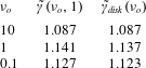
Let us concentrate on our results at
 $\unicode[STIX]{x1D705}=1$
; we have
 $\tilde{\unicode[STIX]{x1D6FE}}(\unicode[STIX]{x1D708}_{o},1)=1.087$
,
 $1.141$
and
 $1.127$
for
 $\unicode[STIX]{x1D708}_{o}=10$
,
 $1$
and
 $0.1$
, respectively, as listed in table 3. These values are respectively in good agreement with the corresponding previous results of
 $\tilde{\unicode[STIX]{x1D6FE}}_{disk}(\unicode[STIX]{x1D708}_{o})$
, which are also shown in table 2. This shows that the drag coefficient of a liquid domain reasonably approaches the one for a rigid disk as
 $\unicode[STIX]{x1D702}_{i}/\unicode[STIX]{x1D702}_{o}$
tends to infinity. In contrast, Rao & Das (Reference Rao and Das2015) did not observe any significant change of the drag coefficient with
 $\unicode[STIX]{x1D705}$
for
 $\unicode[STIX]{x1D705}>0$
. The figure 6(a) of Rao & Das (Reference Rao and Das2015) is obtained from their equation (2.7); this integral equation is discretized into a set of some thousands of simultaneous equations for numerical calculation. In the present study, correspondingly, we can sum up (4.5) from
 $n=0$
to
 $\infty$
and use (4.2) to derive an integral equation with respect to
 $\tilde{A}(\unicode[STIX]{x1D701})$
. This equation contains a term involving
 $\text{J}_{0}$
, unlike (2.7) of Rao & Das (Reference Rao and Das2015). This is because the third term on the right-hand side of (3.7) is not considered in Rao & Das (Reference Rao and Das2015). For comparison, we use our formula to calculate the drag coefficient by putting
 $\unicode[STIX]{x1D6FD}_{n}$
equal to zero as done in Rao & Das (Reference Rao and Das2015). As shown by the dashed-dotted curves in figures 4–6, none of them approaches the result for a rigid disk as
 $\unicode[STIX]{x1D705}$
approaches unity. This means that the third term on the right-hand side of (3.7) is required unless
 $\unicode[STIX]{x1D702}_{i}$
equals
 $\unicode[STIX]{x1D702}_{o}$
, as discussed below equation (3.7).
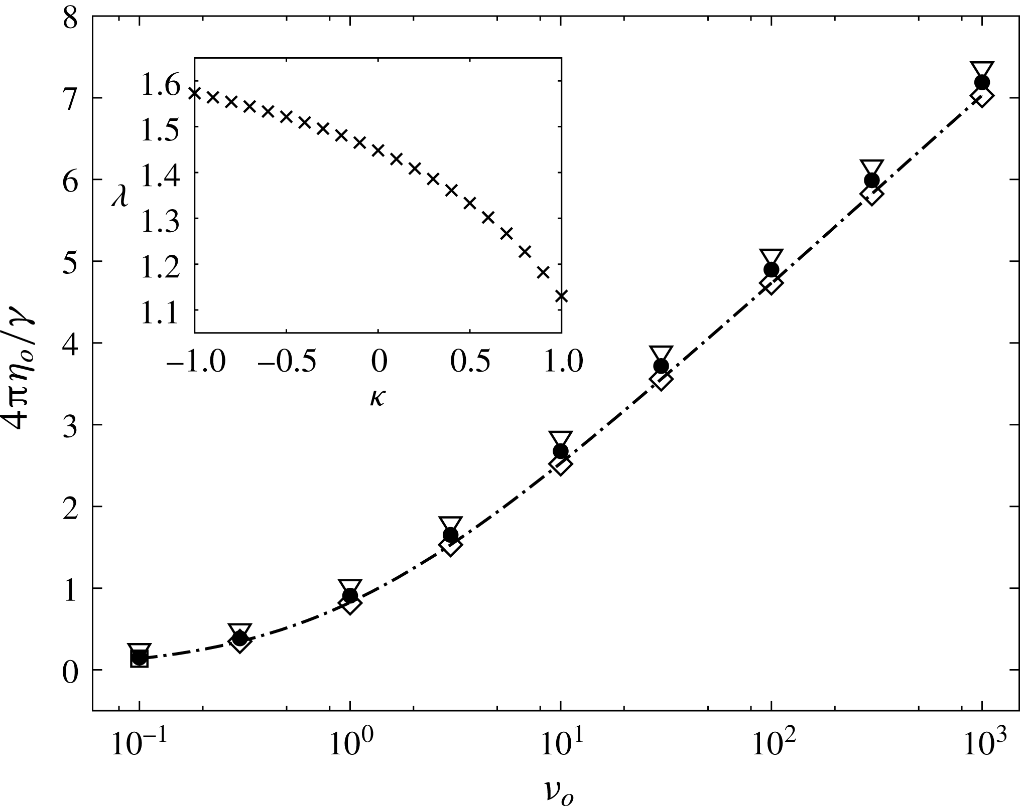
Semi-logarithmic plots of
 $4\unicode[STIX]{x03C0}\unicode[STIX]{x1D702}_{o}/\unicode[STIX]{x1D6FE}$
versus
 $\unicode[STIX]{x1D708}_{o}$
. We use (4.11) and (4.12) to calculate the results for
 $\unicode[STIX]{x1D705}=0$
(triangles),
 $0.5$
(circles) and
 $1$
(diamonds). For each value of
 $\unicode[STIX]{x1D705}$
, line fitting to the data of the three largest values of
 $\unicode[STIX]{x1D708}_{o}$
gives
 $\unicode[STIX]{x1D706}=1.13,1.33$
, and
 $1.45$
, respectively. Dashed-dotted curve represents
 $4\unicode[STIX]{x03C0}\unicode[STIX]{x1D702}_{o}/\unicode[STIX]{x1D6FE}_{disk}$
calculated by using (3.18). A plot of
 $\unicode[STIX]{x1D706}$
against
 $\unicode[STIX]{x1D705}$
is shown in the inset.

The asymptotic forms shown by (3.19) and (3.21) suggest that a
 $\unicode[STIX]{x1D705}$
-dependent constant, denoted by
 $\unicode[STIX]{x1D706}$
, can be defined so that the fraction
 $4\unicode[STIX]{x03C0}\unicode[STIX]{x1D702}_{o}/\unicode[STIX]{x1D6FE}$
is approximately equal to
 $\ln (\unicode[STIX]{x1D706}\unicode[STIX]{x1D708}_{o})$
for
 $\unicode[STIX]{x1D708}_{o}\gg 1$
. Figure 7 shows how the fraction depends on
 $\unicode[STIX]{x1D708}_{o}$
. Each of the symbols in this figure appear along a line as
 $\unicode[STIX]{x1D708}_{o}$
increases in this semi-logarithmic plot, as expected. We can obtain the value of
 $\unicode[STIX]{x1D706}$
from the slope of the line. Using this procedure for various values of
 $\unicode[STIX]{x1D705}$
, we plot
 $\unicode[STIX]{x1D706}$
against
 $\unicode[STIX]{x1D705}$
in the inset. As mentioned above, we need larger
 $N$
when
 $\unicode[STIX]{x1D708}_{o}\ll 1$
. Then, although data are not shown,
 $\unicode[STIX]{x1D6FE}/(4\unicode[STIX]{x03C0}\unicode[STIX]{x1D702}_{o})$
appears proportional to
 $1/\unicode[STIX]{x1D708}_{o}$
for
 $|\unicode[STIX]{x1D705}|\leqslant 1$
, as expected from (3.19) and (3.21).
5 Discussion
By using Saffman & Delbrück’s model with a rigid disk replaced by a circular liquid domain, we obtain its drag coefficient as a power series with respect to
 $\unicode[STIX]{x1D705}$
, as shown in (4.11) and (4.12). Each term of the power series is given by (4.13), which is calculated with the aid of the recurrence relation of (4.5)–(4.7). Fujitani (Reference Fujitani2013a
) calculated the drag coefficient only up to the order of
 $\unicode[STIX]{x1D705}$
in the same model by considering the possibility that the ambient fluids are confined by the walls parallel to the flat membrane. Thus, equation (4.12) is a significant extension of the previous result in the absence of the walls. Numerically calculating the integrals involved in the coefficients in (4.12), we find that truncating the infinite series can give a good approximation of its sum over the region of
 $-1\leqslant \unicode[STIX]{x1D705}\leqslant 1$
, as shown in figures 4–6. In particular, our results for
 $0<\unicode[STIX]{x1D705}<1$
clearly fill the gap between the previous results of Koker (Reference De Koker1996) and Hughes et al. (Reference Hughes, Pailthorpe and White1981), i.e. of
 $\unicode[STIX]{x1D705}=0$
and
 $1$
.
Aliaskarisohi et al. (Reference Aliaskarisohi, Tierno, Dhar, Khattari, Blaszczynski and Fischer2010) calculated the drag coefficient of a circular liquid domain on a spherical membrane by using the Stokes equations for the 3-D fluids and fluid membrane; the above-mentioned gap was not filled, as stated below their equation (5.42). In general, when the membrane is curved, the governing equations are modified, as shown in Aris (Reference Aris1989), Fujitani (Reference Fujitani1994), Powers (Reference Powers2010). Still then, if
 $\unicode[STIX]{x1D702}_{i}\neq \unicode[STIX]{x1D702}_{o}$
, the velocity gradient of the 2-D fluid remains discontinuous across the domain perimeter because this discontinuity comes from the local force balance in the plane tangential to the membrane. The force normal to the membrane does not change the balance. The surface force density at equation (5.5) of Aliaskarisohi et al. (Reference Aliaskarisohi, Tierno, Dhar, Khattari, Blaszczynski and Fischer2010) is conditioned by the stress continuity in the 2-D fluid across the perimeter. It remains, however, to be examined whether or not this conditioned force density generates the required discontinuity in the velocity gradient of the 2-D fluid when the membrane viscosities are not the same inside and outside the domain. Aliaskarisohi et al. (Reference Aliaskarisohi, Tierno, Dhar, Khattari, Blaszczynski and Fischer2010) assumed the same membrane viscosities in analysing their experimental data. As stated at the end of their § 8, they justified this for the reason that, if the domain size, the membrane viscosity outside the domain and the viscosity of the ambient 3-D fluid are given, de Koker’s result is not so much different from that of Hughes et al. (Reference Hughes, Pailthorpe and White1981). It seems in this reason to be conjectured that the drag coefficient changes monotonically as the ratio
 $\unicode[STIX]{x1D702}_{i}/\unicode[STIX]{x1D702}_{o}$
changes from the unity to infinity. This conjecture in a flat membrane is verified by our figures 4–6. Cicuta et al. (Reference Cicuta, Keller and Veatch2007) analysed their data for a circular liquid domain by assuming that its drag coefficient has the same asymptotic form as that of a rigid disk. This assumption is verified by our figure 7.
As mentioned in § 1, the drag coefficient of a droplet in a 3-D fluid was first calculated early in the 20th century (Hadamard Reference Hadamard1911; Rybczynski Reference Rybczynski1911). The result, having been checked experimentally and numerically, is found to be valid when the Reynolds number is small, the Weber number is small and the fluids can be regarded as pure (Clift et al. Reference Clift, Grace and Weber1978; Loth Reference Loth2008). This history gives an example that an exact result in a simple model contributes to our deep understanding of the real-life phenomena. Saffman and Delbrück’s result for a rigid disk has a similar history, as mentioned in § 1. Likewise, our present study on a circular liquid domain is well expected to contribute to our understanding of the real-life phase-separated fluid membrane with the aid of future studies.
It is assumed in our model that the membrane lies in the coexistence phase sufficiently far from the demixing critical point, as mentioned in § 1. Thus, the composition is assumed to be homogeneous in each of the domain interior and exterior, which leads to (2.2)–(2.4). In contrast, the interfacial region between them has a finite thickness if the membrane is close to the critical point. Then, the composition, and thus the viscosity, change gradually across the interfacial region, and the 2-D flow can pass across the interfacial region. This dynamics can be described in terms of the hydrodynamics based on the free-energy functional describing a near-critical fluid mixture. As mentioned in Fujitani (Reference Fujitani2013b ), Okamoto, Fujitani & Komura (Reference Okamoto, Fujitani and Komura2013), Fujitani (Reference Fujitani2016), the stress due to the composition gradient becomes involved in the first entry of (2.2), and the velocity field becomes dependent on the fields of the composition and chemical potential. This complicated dynamics approaches the dynamics of our simple model as the membrane becomes farther from the critical point. Then, the stress due to the composition gradient becomes the line tension, preventing the flow from passing across the interface. Instead, in the simple model, one of the boundary conditions acquires the distinctive feature to be considered carefully, as shown in figure 2. The state considered here may be used as a reference state in considering the drag coefficient of a domain in the membrane closer to the critical point in future.
The calculation procedure for the discontinuity of the velocity gradient only in the 2-D fluid is mentioned in the second paragraph of § 3. Using the procedure, we can also calculate the drag coefficient of a liquid domain in a fluid membrane surrounded by confined 3-D fluids; it was calculated only up to the order of
 $\unicode[STIX]{x1D705}$
in Fujitani (Reference Fujitani2013a
). The procedure can be also applied in calculating small deformation of a liquid domain in a 2-D linear shear flow; it was calculated in Fujitani (Reference Fujitani2005) only for
 $\unicode[STIX]{x1D705}=0$
and the stagnation flow. When we consider the drag coefficient of a dispersed domain in a viscoelastic membrane, a similar discontinuity problem would occur across the perimeter. Our procedure and results should give good starting points for solving this kind of future problem.
Acknowledgements
We thank S. Komura, Y. Ohtsuka and S. L. Das for helpful discussion. Part of the work by Y.F. was financially supported by Keio Gakuji Shinko Shikin.
Appendix A. Some details in deriving (3.5), (3.6) and (3.13)
The derivation of (3.5), (3.6) and (3.13) is described in detail in Fujitani (Reference Fujitani2013a
); some descriptions are repeated here for convenience. Equation (2.1) yields
 $\unicode[STIX]{x0394}P=0$
, which can be transformed as
 $$\begin{eqnarray}\displaystyle (\unicode[STIX]{x2202}_{z}^{2}-\unicode[STIX]{x1D701}^{2})\hat{P}_{m}(\unicode[STIX]{x1D701},z)=0. & & \displaystyle\end{eqnarray}$$
We introduce
 $\tilde{V}_{m}^{\pm }\equiv \tilde{V}_{rm}\pm \text{i}\tilde{V}_{\unicode[STIX]{x1D703}m}$
, whose Hankel transform
 $\hat{V}_{m}^{\pm }$
is defined as
 $$\begin{eqnarray}\displaystyle \hat{V}_{m}^{\pm }(\unicode[STIX]{x1D701},z)\equiv \int _{0}^{\infty }\,\text{d}r\,r\text{J}_{m\pm 1}(\unicode[STIX]{x1D701}r)\tilde{V}_{m}^{\pm }(r,z). & & \displaystyle\end{eqnarray}$$
Using (3.1) and (3.2), we can rewrite the first equation of (2.1) into
 $$\begin{eqnarray}\displaystyle & \displaystyle \unicode[STIX]{x1D707}(\unicode[STIX]{x2202}_{z}^{2}-\unicode[STIX]{x1D701}^{2})\hat{V}_{m}^{\pm }=\mp \unicode[STIX]{x1D701}\hat{P}_{m}\quad \text{and} & \displaystyle\end{eqnarray}$$
 $$\begin{eqnarray}\displaystyle & \displaystyle \unicode[STIX]{x1D707}(\unicode[STIX]{x2202}_{z}^{2}-\unicode[STIX]{x1D701}^{2})\hat{V}_{zm}=\unicode[STIX]{x2202}_{z}\hat{P}_{m}. & \displaystyle\end{eqnarray}$$
The Fourier transform of the incompressibility condition in (2.1) is
 $$\begin{eqnarray}\displaystyle \left(\unicode[STIX]{x2202}_{r}+\frac{m+1}{r}\right)\tilde{V}_{m}^{+}+\left(\unicode[STIX]{x2202}_{r}-\frac{m-1}{r}\right)\tilde{V}_{m}^{-}=-2\unicode[STIX]{x2202}_{z}\hat{V}_{zm}, & & \displaystyle\end{eqnarray}$$
which yields
 $$\begin{eqnarray}\displaystyle \unicode[STIX]{x1D701}\hat{V}_{m}^{+}-\unicode[STIX]{x1D701}\hat{V}_{m}^{-}=-2\unicode[STIX]{x2202}_{z}\hat{V}_{zm}, & & \displaystyle\end{eqnarray}$$
with the aid of the identity
 $$\begin{eqnarray}\displaystyle \left(\unicode[STIX]{x2202}_{r}\mp \frac{m}{r}\right)\text{J}_{m}(\unicode[STIX]{x1D701}r)=\mp \unicode[STIX]{x1D701}\text{J}_{m\pm 1}(\unicode[STIX]{x1D701}r). & & \displaystyle\end{eqnarray}$$
As mentioned below (3.2), we have only to consider the modes of
 $m=\pm 1$
. From the symmetry of the field, we have
 $\hat{P}_{1}=-\hat{P}_{-1}$
and
 $\hat{V}_{\pm 1}^{+}=\hat{V}_{\mp 1}^{-}$
. Equation (A 1) gives
 $$\begin{eqnarray}\displaystyle \hat{P}_{1}=\frac{\unicode[STIX]{x1D701}}{2}D_{1}^{-}(\unicode[STIX]{x1D701})\text{e}^{-\unicode[STIX]{x1D701}|z|}, & & \displaystyle\end{eqnarray}$$
 $$\begin{eqnarray}\displaystyle & \displaystyle \hat{V}_{1}^{\pm }=\frac{1}{2\unicode[STIX]{x1D707}}\left\{D_{1}^{+}(\unicode[STIX]{x1D701})\pm \frac{\unicode[STIX]{x1D701}|z|}{2}D_{1}^{-}(\unicode[STIX]{x1D701})\right\}\text{e}^{-\unicode[STIX]{x1D701}|z|}, & \displaystyle\end{eqnarray}$$
 $$\begin{eqnarray}\displaystyle & \displaystyle \hat{V}_{z1}=\frac{\unicode[STIX]{x1D701}z}{4\unicode[STIX]{x1D707}}D_{1}^{-}(\unicode[STIX]{x1D701})\text{e}^{-\unicode[STIX]{x1D701}|z|}. & \displaystyle\end{eqnarray}$$
Here, the functions
 $D_{1}^{\pm }(\unicode[STIX]{x1D701})$
are to be determined by the equations involved in the membrane.
Combining (2.5) with the second equations of (2.1) and (2.2), we use (A 10) to have
 $$\begin{eqnarray}\displaystyle 0=\lim _{z\rightarrow 0}\frac{\unicode[STIX]{x2202}V_{z}}{\unicode[STIX]{x2202}z}=\lim _{z\rightarrow 0}\frac{\cos \unicode[STIX]{x1D703}}{2\unicode[STIX]{x1D707}}\int _{0}^{\infty }\,\text{d}\unicode[STIX]{x1D701}\,\unicode[STIX]{x1D701}^{2}\text{J}_{1}(\unicode[STIX]{x1D701}r)D_{1}^{-}(\unicode[STIX]{x1D701})\text{e}^{-\unicode[STIX]{x1D701}|z|} & & \displaystyle\end{eqnarray}$$
for
 $r\neq a$
. The second equality of which comes from (A 10). The above yields
 $D_{1}^{-}=0$
, as discussed around (3.11) and (3.27) of Fujitani (Reference Fujitani2013a
). This is reasonable, considering that such a singular velocity field as have non-zero (A 11) only at
 $r=a$
is not expected from (2.1). The Fourier transformation of (2.2) gives
 $$\begin{eqnarray}\displaystyle \unicode[STIX]{x1D702}\left[\frac{1}{r}\unicode[STIX]{x2202}_{r}(r\unicode[STIX]{x2202}_{r})-\frac{(m\pm 1)^{2}}{r^{2}}\right]\tilde{v}_{m}^{\pm }+\tilde{F}_{m}^{\pm }=\left(\unicode[STIX]{x2202}_{r}\mp \frac{m}{r}\right)\tilde{p}_{m}, & & \displaystyle\end{eqnarray}$$
where
 $\tilde{v}_{m}^{\pm }\equiv \tilde{v}_{rm}\pm \text{i}\tilde{v}_{\unicode[STIX]{x1D703}m}$
and
 $\tilde{F}_{m}^{\pm }\equiv \tilde{F}_{rm}\pm \text{i}\tilde{F}_{\unicode[STIX]{x1D703}m}$
. Here, we can utilize the inverse Hankel transformation of (A 9) in (A 12) because of (2.5). We also utilize
 $$\begin{eqnarray}\displaystyle & \displaystyle F_{r}=2\unicode[STIX]{x1D707}\lim _{z\rightarrow 0+}\frac{\unicode[STIX]{x2202}V_{r}}{\unicode[STIX]{x2202}z}\quad \text{and} & \displaystyle\end{eqnarray}$$
 $$\begin{eqnarray}\displaystyle & \displaystyle F_{\unicode[STIX]{x1D703}}=2\unicode[STIX]{x1D707}\lim _{z\rightarrow 0+}\frac{\unicode[STIX]{x2202}V_{\unicode[STIX]{x1D703}}}{\unicode[STIX]{x2202}z}, & \displaystyle\end{eqnarray}$$
where the factor
 $2$
comes because the 3-D fluids are on both sides. Deleting
 $\tilde{p}_{1}$
from (A 12) for
 $m=1$
, we arrive at
 $$\begin{eqnarray}\displaystyle 0=\int _{0}^{\infty }\,\text{d}\unicode[STIX]{x1D701}\,\unicode[STIX]{x1D701}^{3}D_{1}^{+}(\unicode[STIX]{x1D701})\left(1+\frac{\unicode[STIX]{x1D702}}{2\unicode[STIX]{x1D707}}\unicode[STIX]{x1D701}\right)\text{J}_{1}(\unicode[STIX]{x1D701}r) & & \displaystyle\end{eqnarray}$$
for
 $0\leqslant r<a$
and
 $a<r$
. Equation (A 15) yields (3.5) and (3.6) with
 $A(\unicode[STIX]{x1D701})$
being defined as
 $$\begin{eqnarray}\displaystyle A(\unicode[STIX]{x1D701})=2\unicode[STIX]{x1D701}(1+\unicode[STIX]{x1D708}_{o}\unicode[STIX]{x1D701})D_{1}^{+}(\unicode[STIX]{x1D701}/a). & & \displaystyle\end{eqnarray}$$
Equation (3.6) is derived so that it can be written in terms of
 $\unicode[STIX]{x1D705}$
; equation (3.7) does not give the induced forces. In Fujitani (Reference Fujitani2013a
), the 3-D fluid on each side of the membrane is assumed to be confined by the membrane and a wall, which is parallel to the membrane and lies at the distance
 $Ha$
from the membrane. Equations (3.5) and (3.6) are derived by taking the limit of
 $H\rightarrow \infty$
in (3.1) and (3.2) of Fujitani (Reference Fujitani2013a
). Equation (3.4) corresponds with equation (2.37) of Fujitani (Reference Fujitani2013a
) because of (2.26), (3.8) and (3.13) there.
The
 $x$
-component of
 $\boldsymbol{F}$
is given by
 $$\begin{eqnarray}\displaystyle \int _{0}^{R}\,\text{d}r\,r\int _{0}^{2\unicode[STIX]{x03C0}}\,\text{d}\unicode[STIX]{x1D703}(F_{r}\cos \unicode[STIX]{x1D703}-F_{\unicode[STIX]{x1D703}}\sin \unicode[STIX]{x1D703})=2\unicode[STIX]{x03C0}\int _{0}^{R}r(\tilde{F}_{r1}-\text{i}\tilde{F}_{\unicode[STIX]{x1D703}1}), & & \displaystyle\end{eqnarray}$$
into which (A 13) and (A 14) can be substituted. That of the force exerted on the domain by the membrane outside the domain is given by
 $$\begin{eqnarray}\displaystyle a\int _{0}^{2\unicode[STIX]{x03C0}}\,\text{d}\unicode[STIX]{x1D703}(\unicode[STIX]{x1D70F}_{rr}\cos \unicode[STIX]{x1D703}-\unicode[STIX]{x1D70F}_{r\unicode[STIX]{x1D703}}\sin \unicode[STIX]{x1D703})=2\unicode[STIX]{x03C0}a(\tilde{\unicode[STIX]{x1D70F}}_{rr1}-\text{i}\tilde{\unicode[STIX]{x1D70F}}_{r\unicode[STIX]{x1D703}1}), & & \displaystyle\end{eqnarray}$$
where the Fourier transforms are given by
 $$\begin{eqnarray}\displaystyle & \displaystyle \tilde{\unicode[STIX]{x1D70F}}_{rr1}=-\tilde{p}_{1}+2\unicode[STIX]{x1D702}\frac{\unicode[STIX]{x2202}\tilde{v}_{r1}}{\unicode[STIX]{x2202}r} & \displaystyle\end{eqnarray}$$
and
 $$\begin{eqnarray}\displaystyle & \displaystyle \tilde{\unicode[STIX]{x1D70F}}_{r\unicode[STIX]{x1D703}1}=\text{i}\frac{\unicode[STIX]{x1D702}}{r}\tilde{v}_{r1}+\unicode[STIX]{x1D702}\frac{\unicode[STIX]{x2202}\tilde{v}_{\unicode[STIX]{x1D703}1}}{\unicode[STIX]{x2202}r}-\frac{\unicode[STIX]{x1D702}}{r}\tilde{v}_{\unicode[STIX]{x1D703}1}. & \displaystyle\end{eqnarray}$$
In particular, as is found from (3.10) of Fujitani (Reference Fujitani2013a ), we have
 $$\begin{eqnarray}\displaystyle \tilde{\unicode[STIX]{x1D70F}}_{r\unicode[STIX]{x1D703}1}=\frac{-\text{i}\unicode[STIX]{x1D702}}{4\unicode[STIX]{x1D707}a^{3}}\int _{0}^{\infty }\,\text{d}\unicode[STIX]{x1D701}\frac{\unicode[STIX]{x1D701}J_{2}^{\prime }(\unicode[STIX]{x1D701}R)A(\unicode[STIX]{x1D701})}{1+\unicode[STIX]{x1D708}_{o}\unicode[STIX]{x1D701}}. & & \displaystyle\end{eqnarray}$$
Using (A 17) and (A 18), we find the total force along the
 $x$
-axis to be given by
 $$\begin{eqnarray}\displaystyle {\mathcal{F}}_{x}=\lim _{R\rightarrow 1+}\lim _{Z\rightarrow 0+}\left[-\frac{\unicode[STIX]{x03C0}}{a}\int _{0}^{\infty }\,\text{d}\unicode[STIX]{x1D701}\unicode[STIX]{x1D701}J_{2}(\unicode[STIX]{x1D701}R)A(\unicode[STIX]{x1D701})\text{e}^{-\unicode[STIX]{x1D701}Z}\right], & & \displaystyle\end{eqnarray}$$
which is divided by
 $-U$
to yield the drag coefficient (3.13). This is also derived from (2.24), (2.41) and (3.13) of Fujitani (Reference Fujitani2013a
), whose (3.40) is helpful in deriving (4.13). The convergence factor
 $\text{e}^{-\unicode[STIX]{x1D701}Z}$
comes from that of (A 9) and cannot be neglected because
 $A(\unicode[STIX]{x1D701})$
contains a term proportional to
 $\text{J}_{0}(\unicode[STIX]{x1D701})$
. Precisely speaking, each integrand of (3.5) and (3.6) also has this factor, as mentioned below (3.24) of Fujitani (Reference Fujitani2013a
). This helps in driving (3.8).
Considering (3.9), we find that the third term on the right-hand side of (3.7) makes (A 21) have a term proportional to the product of
 $\unicode[STIX]{x1D702}$
and the integral in the second entry of (4.8). This integral is discontinuous across
 $R=1$
, as mentioned in appendix B. Its negative is the integral of (3.26) of Fujitani (Reference Fujitani2013a
) in the limit of
 $H\rightarrow \infty$
, and Fujitani (Reference Fujitani2013a
, figure 2) shows discontinuity of this integral across
 $R=1$
. In passing, whether the membrane is tensionless or not is relevant to the shape fluctuation (Shiba, Noguchi & Fournier Reference Shiba, Noguchi and Fournier2016), but does not change the formulation in the present study because the Stokes equations and the drag force remain unchanged even if the constant pressure is added to
 $p$
.
Appendix B. Derivation of (4.5) and (4.7)
We expand
 $c_{1}$
and
 $c_{2}$
in (3.9) with respect to
 $\unicode[STIX]{x1D705}$
as
 $$\begin{eqnarray}c_{1}=\frac{2\unicode[STIX]{x1D707}a^{2}U}{Y_{0}(\unicode[STIX]{x1D708}_{o})}\mathop{\sum }_{n=0}^{\infty }\unicode[STIX]{x1D6FC}_{n}^{\sharp }\unicode[STIX]{x1D705}^{n}\quad \text{and}\quad c_{2}=-\frac{2\unicode[STIX]{x1D707}a^{2}U}{Y_{0}(\unicode[STIX]{x1D708}_{o})}\mathop{\sum }_{n=0}^{\infty }\unicode[STIX]{x1D6FD}_{n}\unicode[STIX]{x1D705}^{n},\end{eqnarray}$$
where
 $\unicode[STIX]{x1D6FC}_{n}^{\sharp }$
and
 $\unicode[STIX]{x1D6FD}_{n}$
are the expansion coefficients independent of
 $\unicode[STIX]{x1D705}$
. Because of (3.14), we have
 $\unicode[STIX]{x1D6FC}_{0}^{\sharp }=1$
. Substituting (4.1) and (4.2) into (3.9) yields (4.5), where
 $\unicode[STIX]{x1D6FC}_{n}$
is given by
 $$\begin{eqnarray}\displaystyle \unicode[STIX]{x1D6FC}_{n}=\unicode[STIX]{x1D6FC}_{n}^{\sharp }-\int _{0}^{\infty }\,\text{d}\unicode[STIX]{x1D709}\frac{\unicode[STIX]{x1D709}\text{J}_{0}(\unicode[STIX]{x1D709})}{1+\unicode[STIX]{x1D708}_{o}\unicode[STIX]{x1D709}}\tilde{A}_{n-1}(\unicode[STIX]{x1D709}). & & \displaystyle\end{eqnarray}$$
As shown (3.28) of Fujitani (Reference Fujitani2013a
), the integral in the second equation of (4.8) jumps by
 $1/\unicode[STIX]{x1D708}_{o}$
as
 $R$
increases across unity. Substituting (4.1), (4.2) and (4.5) into (A 21), we find that (2.6) gives
 $$\begin{eqnarray}\displaystyle \mathop{\sum }_{n=0}^{\infty }\unicode[STIX]{x1D6FD}_{n}\left(-\unicode[STIX]{x1D705}{\mathcal{G}}+\frac{1}{\unicode[STIX]{x1D708}_{o}}\right)\unicode[STIX]{x1D705}^{n}=\mathop{\sum }_{n=0}^{\infty }(\unicode[STIX]{x1D6FC}_{n}\hat{N}\tilde{A}_{0}+\unicode[STIX]{x1D705}\hat{N}\hat{M}\tilde{A}_{n})\unicode[STIX]{x1D705}^{n+1}, & & \displaystyle\end{eqnarray}$$
which yields (4.7).
Appendix C. Numerical procedure for
 $\unicode[STIX]{x1D6E9}\hat{M}\text{J}_{0}$

The integral
 $[\hat{M}\text{J}_{0}](\unicode[STIX]{x1D701})$
is given by (4.4) with
 $f$
being replaced by
 $\text{J}_{0}$
. It contains the factor
 $\unicode[STIX]{x1D709}/(1+\unicode[STIX]{x1D708}_{o}\unicode[STIX]{x1D709})$
. Rewriting this factor in the way mentioned in the first paragraph of § 4.2, we find the integral to be given by
 $\unicode[STIX]{x1D708}_{o}^{-1}$
multiplied by the sum of two integrals. One is
 $$\begin{eqnarray}\displaystyle \int _{0}^{\infty }\,\text{d}\unicode[STIX]{x1D709}\frac{\unicode[STIX]{x1D701}\text{J}_{0}(\unicode[STIX]{x1D709})\text{J}_{1}(\unicode[STIX]{x1D701})-\unicode[STIX]{x1D709}\text{J}_{0}(\unicode[STIX]{x1D701})\text{J}_{1}(\unicode[STIX]{x1D709})}{\unicode[STIX]{x1D701}^{2}-\unicode[STIX]{x1D709}^{2}}\text{J}_{0}(\unicode[STIX]{x1D709}), & & \displaystyle\end{eqnarray}$$
while the rest depends on
 $\unicode[STIX]{x1D708}_{o}$
. The latter, denoted by
 $\hat{M}_{r}\text{J}_{0}$
, is numerically found to be approximately proportional to
 $$\begin{eqnarray}\displaystyle E(\unicode[STIX]{x1D701},\unicode[STIX]{x1D6FF})\equiv \frac{\cos (\unicode[STIX]{x1D701}+\unicode[STIX]{x1D6FF})}{\unicode[STIX]{x1D701}\sqrt{\unicode[STIX]{x1D701}}} & & \displaystyle\end{eqnarray}$$
for large
 $\unicode[STIX]{x1D701}$
. The function
 $E$
is defined here. The constant of proportion, denoted by
 $C$
, and the constant
 $\unicode[STIX]{x1D6FF}$
are to be fixed numerically. Because
 $\unicode[STIX]{x1D6FF}$
is close to
 $\unicode[STIX]{x03C0}/4$
, as suggested in Fujitani (Reference Fujitani2012, §3), it is numerically convenient to use
 $$\begin{eqnarray}\unicode[STIX]{x1D6E9}\hat{M}_{r}\text{J}_{0}=\unicode[STIX]{x1D6E9}\left(\hat{M}_{r}\text{J}_{0}-CE\left(\unicode[STIX]{x1D701},\frac{\unicode[STIX]{x03C0}}{4}\right)\right)-C\sqrt{\frac{\unicode[STIX]{x03C0}}{2}}.\end{eqnarray}$$
We can calculate the first term on the right-hand side above rather easily by putting the upper bound of the integral equal to
 $10^{6}$
. It is numerically found that
 $\hat{M}\tilde{B}_{n}$
has the same asymptotic form as
 $\hat{M}_{r}\text{J}_{0}$
. Thus, we can use this form to check the numerical results of integrals of
 $\hat{M}\tilde{B}_{n}$
obtained by the way mentioned in § 4.2. In contrast, equation (C 1) turns out to be approximately proportional to
 $E(\unicode[STIX]{x1D701},\unicode[STIX]{x1D6FF}_{p})[\ln \unicode[STIX]{x1D701}]^{0.8}$
for large
 $\unicode[STIX]{x1D701}$
, where
 $\unicode[STIX]{x1D6FF}_{p}$
is a constant to be fixed numerically. The term resulting from the operation of
 $\unicode[STIX]{x1D6E9}$
on (C 1) is rewritten by using (3.40) of Fujitani (Reference Fujitani2013a
), and then calculated numerically with the upper bound of the integral put equal to
 $10^{7}$
. Because of the logarithmic dependence,
 $[\hat{N}\hat{M}\text{J}_{0}](R)$
is discontinuous at
 $R=1$
.
We find
 $\unicode[STIX]{x1D6E9}\hat{M}\text{J}_{0}=1.02\times 10^{-1}$
,
 $4.94\times 10^{-1}$
and
 $9.35\times 10^{-1}$
for
 $\unicode[STIX]{x1D708}_{o}=10$
, 1 and 0.1, respectively. For
 $n\geqslant 2$
, in our numerical results of (4.13),
 $\unicode[STIX]{x1D6E9}\hat{M}\tilde{A}_{n-1}$
is negative while
 $\unicode[STIX]{x1D6FC}_{n}+2\unicode[STIX]{x1D6FD}_{n}$
is positive, and the ratio of the former to the latter in magnitude remains approximately 0.23 and 0.38 for
 $\unicode[STIX]{x1D708}_{o}=10$
and 1, respectively. The ratio for
 $\unicode[STIX]{x1D708}_{o}=0.1$
is approximately 0.51 for
 $n=2$
, and decreases to approximately 0.29 for
 $n\geqslant 10$
. In contrast, the ratio for
 $n=1$
is larger than unity for these values of
 $\unicode[STIX]{x1D708}_{o}$
.