





%20--%3e%3c!DOCTYPE%20svg%20PUBLIC%20'-//W3C//DTD%20SVG%201.0//EN'%20'http://www.w3.org/TR/2001/REC-SVG-20010904/DTD/svg10.dtd'%3e%3csvg%20version='1.0'%20id='Layer_1'%20xmlns='http://www.w3.org/2000/svg'%20xmlns:xlink='http://www.w3.org/1999/xlink'%20x='0px'%20y='0px'%20width='64px'%20height='64px'%20viewBox='5.5%20-3.5%2064%2064'%20enable-background='new%205.5%20-3.5%2064%2064'%20xml:space='preserve'%3e%3cg%3e%3ccircle%20fill='%23FFFFFF'%20fill-opacity='0'%20cx='37.785'%20cy='28.501'%20r='28.836'/%3e%3cpath%20fill='%23595959'%20d='M37.441-3.5c8.951,0,16.572,3.125,22.857,9.372c3.008,3.009,5.295,6.448,6.857,10.314%20c1.561,3.867,2.344,7.971,2.344,12.314c0,4.381-0.773,8.486-2.314,12.313c-1.543,3.828-3.82,7.21-6.828,10.143%20c-3.123,3.085-6.666,5.448-10.629,7.086c-3.961,1.638-8.057,2.457-12.285,2.457s-8.276-0.808-12.143-2.429%20c-3.866-1.618-7.333-3.961-10.4-7.027c-3.067-3.066-5.4-6.524-7-10.372S5.5,32.767,5.5,28.5c0-4.229,0.809-8.295,2.428-12.2%20c1.619-3.905,3.972-7.4,7.057-10.486C21.08-0.394,28.565-3.5,37.441-3.5z%20M37.557,2.272c-7.314,0-13.467,2.553-18.458,7.657%20c-2.515,2.553-4.448,5.419-5.8,8.6c-1.354,3.181-2.029,6.505-2.029,9.972c0,3.429,0.675,6.734,2.029,9.913%20c1.353,3.183,3.285,6.021,5.8,8.516c2.514,2.496,5.351,4.399,8.515,5.715c3.161,1.314,6.476,1.971,9.943,1.971%20c3.428,0,6.75-0.665,9.973-1.999c3.219-1.335,6.121-3.257,8.713-5.771c4.99-4.876,7.484-10.99,7.484-18.344%20c0-3.543-0.648-6.895-1.943-10.057c-1.293-3.162-3.18-5.98-5.654-8.458C50.984,4.844,44.795,2.272,37.557,2.272z%20M37.156,23.187%20l-4.287,2.229c-0.458-0.951-1.019-1.619-1.685-2c-0.667-0.38-1.286-0.571-1.858-0.571c-2.856,0-4.286,1.885-4.286,5.657%20c0,1.714,0.362,3.084,1.085,4.113c0.724,1.029,1.791,1.544,3.201,1.544c1.867,0,3.181-0.915,3.944-2.743l3.942,2%20c-0.838,1.563-2,2.791-3.486,3.686c-1.484,0.896-3.123,1.343-4.914,1.343c-2.857,0-5.163-0.875-6.915-2.629%20c-1.752-1.752-2.628-4.19-2.628-7.313c0-3.048,0.886-5.466,2.657-7.257c1.771-1.79,4.009-2.686,6.715-2.686%20C32.604,18.558,35.441,20.101,37.156,23.187z%20M55.613,23.187l-4.229,2.229c-0.457-0.951-1.02-1.619-1.686-2%20c-0.668-0.38-1.307-0.571-1.914-0.571c-2.857,0-4.287,1.885-4.287,5.657c0,1.714,0.363,3.084,1.086,4.113%20c0.723,1.029,1.789,1.544,3.201,1.544c1.865,0,3.18-0.915,3.941-2.743l4,2c-0.875,1.563-2.057,2.791-3.541,3.686%20c-1.486,0.896-3.105,1.343-4.857,1.343c-2.896,0-5.209-0.875-6.941-2.629c-1.736-1.752-2.602-4.19-2.602-7.313%20c0-3.048,0.885-5.466,2.658-7.257c1.77-1.79,4.008-2.686,6.713-2.686C51.117,18.558,53.938,20.101,55.613,23.187z'/%3e%3c/g%3e%3c/svg%3e)
%20--%3e%3c!DOCTYPE%20svg%20PUBLIC%20'-//W3C//DTD%20SVG%201.0//EN'%20'http://www.w3.org/TR/2001/REC-SVG-20010904/DTD/svg10.dtd'%3e%3csvg%20version='1.0'%20id='Layer_1'%20xmlns='http://www.w3.org/2000/svg'%20xmlns:xlink='http://www.w3.org/1999/xlink'%20x='0px'%20y='0px'%20width='64px'%20height='64px'%20viewBox='5.5%20-3.5%2064%2064'%20enable-background='new%205.5%20-3.5%2064%2064'%20xml:space='preserve'%3e%3cg%3e%3ccircle%20fill='%23FFFFFF'%20fill-opacity='0'%20cx='37.637'%20cy='28.806'%20r='28.276'/%3e%3cg%3e%3cpath%20fill='%23595959'%20d='M37.443-3.5c8.988,0,16.57,3.085,22.742,9.257C66.393,11.967,69.5,19.548,69.5,28.5c0,8.991-3.049,16.476-9.145,22.456%20C53.879,57.319,46.242,60.5,37.443,60.5c-8.649,0-16.153-3.144-22.514-9.43C8.644,44.784,5.5,37.262,5.5,28.5%20c0-8.761,3.144-16.342,9.429-22.742C21.101-0.415,28.604-3.5,37.443-3.5z%20M37.557,2.272c-7.276,0-13.428,2.553-18.457,7.657%20c-5.22,5.334-7.829,11.525-7.829,18.572c0,7.086,2.59,13.22,7.77,18.398c5.181,5.182,11.352,7.771,18.514,7.771%20c7.123,0,13.334-2.607,18.629-7.828c5.029-4.838,7.543-10.952,7.543-18.343c0-7.276-2.553-13.465-7.656-18.571%20C50.967,4.824,44.795,2.272,37.557,2.272z%20M46.129,20.557v13.085h-3.656v15.542h-9.944V33.643h-3.656V20.557%20c0-0.572,0.2-1.057,0.599-1.457c0.401-0.399,0.887-0.6,1.457-0.6h13.144c0.533,0,1.01,0.2,1.428,0.6%20C45.918,19.5,46.129,19.986,46.129,20.557z%20M33.042,12.329c0-3.008,1.485-4.514,4.458-4.514s4.457,1.504,4.457,4.514%20c0,2.971-1.486,4.457-4.457,4.457S33.042,15.3,33.042,12.329z'/%3e%3c/g%3e%3c/g%3e%3c/svg%3e)
1. Introduction
Buoyant plumes are found in a wide range of naturally occurring phenomena (e.g. volcanic eruptions, hydrothermal vents and fire plumes) and engineering applications (e.g. heat treatment processes, desalination plants and space heaters). The distinguishing feature of these flows is the presence of a dominant buoyant force resulting from density variations in the presence of a gravitational field (Lee & Chu Reference Lee and Chu2012). In each of these flows, when lower-density fluid is injected into higher-density ambient fluid, the plume contracts laterally, producing large coherent vortical structures that rise vertically, opposite to the direction of gravity. This process repeats continuously, resulting in a characteristic ‘puffing’ behaviour (Bharadwaj & Das Reference Bharadwaj and Das2017). Although this is sometimes referred to as flame ‘flickering’ for laminar reacting plumes (Moreno-Boza et al. Reference Moreno-Boza, Coenen, Sevilla, Carpio, Sánchez and Liñán2016), we will refer to this phenomenon as the puffing instability regardless of whether or not reactions and heat release are present. The frequency at which vortices are shed is the most commonly studied characteristic of this instability, and much research has been devoted to developing scaling relations for the frequency based on plume inlet parameters.
Early research on the puffing instability was focused primarily on reacting plumes, motivated by the need to characterize and mitigate risks associated with fire spread. In reacting plumes, the puffing instability affects the flame height and mixing of fuel and oxidizer, both of which are particularly important for fires in enclosed spaces. As reviewed by Zukoski (Reference Zukoski1986) and Cetegen & Ahmed (Reference Cetegen and Ahmed1993), a key finding of these studies was that the puffing frequency  $f$ is related to the plume radius
 $R_0$ as
 $f\sim R_0^{-1/2}$. It was hypothesized that buoyancy was the dynamical mechanism for generating such behaviour, but an unambiguous definition of the buoyancy force in reacting plumes is difficult due to the spatial variability of density differences resulting from reactions. As a result, the precise physical mechanism that connects frequency scaling relations to the underlying governing equations remains unknown. Elucidating this mechanism is an important ongoing direction of research on reacting plumes, in particular, since similar relations are now being determined empirically in less ideal configurations (e.g. with non-axisymmetric geometries and heterogeneous fuel sources) such as wildfires (Finney et al. Reference Finney, Cohen, Forthofer, McAllister, Gollner, Gorham, Saito, Akafuah, Adam and English2015).
To better understand reacting plume structure and dynamics, it has been common for the past several decades to instead study non-reacting buoyant plumes where complexities associated with chemical reactions are absent, while the essential buoyancy-driven plume dynamics are retained. Much of this research has focused on relating inlet-based parameters (e.g. inflow velocity, density ratio, etc.) to the puffing frequency. Early experimental work by Cetegen & Kasper (Reference Cetegen and Kasper1996) found that the non-dimensional puffing frequency – or Strouhal number,  ${St}_0 \equiv f R_0/U_0$ – could be predicted accurately using the Richardson number
 ${Ri}_0 \equiv (1-\rho _0/\rho _\infty ) gR_0/U_0^{2}$. This result was later generalized by Wimer et al. (Reference Wimer, Lapointe, Christopher, Nigam, Hayden, Upadhye, Strobel, Rieker and Hamlington2020), leading to a proposed relationship for axisymmetric round plumes of the form
 \begin{equation} {St}_0 = 2\,{\rm e}^{{-}1} \left(\frac{{Ri}_0}{2}\right)^{2/5}, \end{equation}
where  $\rho _0$ is the density of the injected fluid,
 $\rho _\infty >\rho _0$ is the density of the surrounding fluid,
 $g$ is the gravitational acceleration, and
 $U_0$ is the velocity of the injected fluid. Equation (1.1) was further substantiated using data from prior experiments (O'Hern et al. Reference O'Hern, Weckman, Gerhart, Tieszen and Schefer2005; Bharadwaj & Das Reference Bharadwaj and Das2017, Reference Bharadwaj and Das2019), stability analyses (Bharadwaj & Das Reference Bharadwaj and Das2017; Chakravarthy, Lesshafft & Huerre Reference Chakravarthy, Lesshafft and Huerre2018; Bharadwaj & Das Reference Bharadwaj and Das2019, Reference Bharadwaj and Das2021), high-resolution simulations (Jiang & Luo Reference Jiang and Luo2000; Wimer et al. Reference Wimer, Day, Lapointe, Meehan, Makowiecki, Glusman, Daily, Rieker and Hamlington2021), and large-eddy simulations (DesJardin, O'Hern & Tieszen Reference DesJardin, O'Hern and Tieszen2004; Burton Reference Burton2009). The density ratio
 $\rho _0/\rho _\infty$ and Froude number
 ${Fr}_0=U_0/(gR_0)^{1/2}$ have also been found to independently affect the puffing frequency (Soteriou, Dong & Cetegen Reference Soteriou, Dong and Cetegen2002; Bharadwaj & Das Reference Bharadwaj and Das2017), but are more commonly combined to obtain relations for
 ${St}_0$ in terms of
 ${Ri}_0$ alone, as in (1.1).
By contrast to  ${Ri}_0$, the puffing frequency has generally been found to have little dependence on the Reynolds number
 ${Re}_0=R_0 U_0/\nu _0$, where
 $\nu _0$ is the kinematic viscosity of the injected fluid (Subbarao & Cantwell Reference Subbarao and Cantwell1992; Bharadwaj & Das Reference Bharadwaj and Das2017). For small density ratios and small
 ${Fr}_0$ (corresponding to large
 ${Ri}_0$), Satti & Agrawal (Reference Satti and Agrawal2006) and Bharadwaj & Das (Reference Bharadwaj and Das2017) found that
 ${Re}_0$ affects only the flow near the viscous limit where the flow transitions from steady to unsteady. The lack of an
 ${Re}_0$ effect is particularly noteworthy given that puffing exists in the limit of low and high
 ${Re}_0$, and between these limits, the flow undergoes a transition between laminar and turbulent behaviours. This transition is distinguished by chaotic, irregular motions as the puffing instability becomes more turbulent due to the interaction of newly formed small-scale structures and the global puffing mode (Subbarao & Cantwell Reference Subbarao and Cantwell1992). The robustness of the puffing frequency through this transition suggests that
 ${Re}_0$ and, by extension, small-scale effects do not impact the global frequency.
At the same time, research on Rayleigh–Taylor instabilities, which are relevant to buoyant plumes where lower-density fluid is injected into higher-density fluid, has shown that the perturbation Reynolds number (closely related to  ${Re}_0$) determines whether the flow transitions between different growth regimes (Wei & Livescu Reference Wei and Livescu2012; Bian et al. Reference Bian, Aluie, Zhao, Zhang and Livescu2020). When the plume undergoes this transition, we expect that as
 ${Re}_0$ increases, the puffing behaviour will undergo a series of complex changes in its temporal evolution, starting with correlated variables at low
 ${Re}_0$, and ending with little to no correlation at high
 ${Re}_0$. This transition has been discussed qualitatively by other researchers (Subbarao & Cantwell Reference Subbarao and Cantwell1992; Cetegen & Kasper Reference Cetegen and Kasper1996), but the implications of this transition on the temporal characteristics of buoyant plumes have yet to be examined in detail.
Rigorously testing the effect of  ${Re}_0$ on buoyant plume structure and dynamics is made difficult by the challenge of controlling
 ${Re}_0$ experimentally, as well as by the high computational cost of fully resolved numerical simulations over a range of
 ${Re}_0$. From an experimental standpoint, most researchers vary
 $U_0$ and
 $R_0$ to keep
 ${Ri}_0$ fixed. However, without considerable caution, varying
 $R_0$ can lead to variations in other non-dimensional numbers, such as the non-dimensional ratio
 $R_0/\phi$, where
 $\phi$ is a measure of the boundary layer width at the inflow plane (Michalke Reference Michalke1984; Nichols, Schmid & Riley Reference Nichols, Schmid and Riley2007). From a computational standpoint, it is easier to ensure that all non-dimensional parameters remain fixed, but most such studies have needed to sacrifice some level of fidelity to perform systematic parameter sweeps. This includes reduced spatial dimensionality (i.e. conducting simulations in two dimensions; Soteriou et al. Reference Soteriou, Dong and Cetegen2002), using stability analyses (Bharadwaj & Das Reference Bharadwaj and Das2017), and using subgrid-scale models (DesJardin et al. Reference DesJardin, O'Hern and Tieszen2004). It is conceivable that these simplifications cause
 ${Re}_0$ to have a reduced impact due to, for example, the discrepancy in spectral kinetic energy transfer in two and three dimensions (Kraichnan Reference Kraichnan1967) or the challenge in performing physically accurate simulations of buoyancy-driven flows using large-eddy simulations (DesJardin et al. Reference DesJardin, O'Hern and Tieszen2004; Nicolette et al. Reference Nicolette, Tieszen, Black, Domino and O'Hern2005).
In the present study, we use three-dimensional (3-D) numerical simulations to examine how  ${Ri}_0$ and
 ${Re}_0$ affect the near-field temporal evolution of helium buoyant plumes. The three-dimensionality of the simulations is important to capture vortex breakdown properly, which has been shown in buoyant plumes to occur abruptly as a function of vertical distance (Subbarao & Cantwell Reference Subbarao and Cantwell1992). To ensure fully resolved yet computational tractable simulations, we use PeleLM (Nonaka, Day & Bell Reference Nonaka, Day and Bell2018), a massively parallel low-Mach hydrodynamics code that solves the governing equations on a dynamically varying and flow-dependent numerical grid. This dynamic grid approach, commonly known as adaptive mesh refinement (AMR), allows us to resolve small-scale flow features locally. This is particularly attractive for buoyant plumes because a large computational domain is required to entrain ambient fluid properly, but grid resolution demands are quite large for localized concentrations of steep gradients (e.g. along the helium–air interface).
The text is organized as follows. A detailed description of the numerical simulations is provided in § 2. We then present simulation results in § 3. Finally, a number of important conclusions drawn from this work are put forth in § 4.
2. Numerical simulations
2.1. Governing equations
We use PeleLM (Nonaka et al. Reference Nonaka, Day and Bell2018) to perform 3-D numerical simulations of helium buoyant plumes. PeleLM solves low-Mach governing equations for continuity, momentum, species and enthalpy, given as (Rehm & Baum Reference Rehm and Baum1978; Majda & Sethian Reference Majda and Sethian1985)
 \begin{gather} \frac{\partial {\rho}}{\partial {t}} + \frac{\partial {(\rho u_i)}}{\partial {x_i}} = 0, \end{gather}
 \begin{gather} \frac{\partial {u_i}}{\partial {t}} + u_j\,\frac{\partial {u_i}}{\partial {x_j}} ={-}\frac{1}{\rho}\,\frac{\partial {\rm \pi}}{\partial {x_i}} + g_i + \frac{1}{\rho}\, \frac{\partial {}}{\partial {x_j}} \left[ \mu \left( \frac{\partial {u_i}}{\partial {x_j}} + \frac{\partial {u_j}}{\partial {x_i}} - \frac{2}{3}\,\delta_{ij}\, \frac{\partial {u_k}}{\partial {x_k}} \right) \right], \end{gather}
 \begin{gather} \frac{\partial {(\rho Y_m)}}{\partial {t}} + \frac{\partial {(\rho u_i Y_m)}}{\partial {x_i}} = \frac{\partial {\varGamma_{mi}}}{\partial {x_i}}, \end{gather}
 \begin{gather} \frac{\partial {(\rho h)}}{\partial {t}} + \frac{\partial {(\rho u_i h)}}{\partial {x_i}} = \frac{\partial {}}{\partial {x_i}}\left(\lambda\,\frac{\partial {T}}{\partial {x_i}} \right) + \frac{\partial {}}{\partial {x_i}} \left(\sum_m h_m \varGamma_{mi}\right). \end{gather}
Here,  $\rho$ is the density,
 $u_i$ are the velocity components,
 ${\rm \pi}$ is the perturbational pressure,
 $g_i$ is gravity,
 $\mu$ is the dynamic viscosity,
 $\delta _{ij}$ is the Kronecker delta function,
 $Y_m$ is the mass fraction of species
 $m$,
 $h$ is the mixture-averaged enthalpy,
 $\lambda$ is the thermal diffusivity,
 $T$ is the temperature, and
 $h_m$ is the enthalpy of species
 $m$. The diffusive flux is defined as
 \begin{equation} \varGamma_{mi} \equiv \rho D_m\,\frac{W_{mix}}{W_m}\,\frac{\partial {Y_m}}{\partial {x_i}}, \end{equation}
where  $D_m$ is the diffusivity,
 $W_m$ is the molecular weight of species
 $m$, and
 $W_{mix}$ is the mixture-averaged molecular weight,
 $W_{mix} \equiv (\sum _m Y_m/W_m)^{-1}$. It is assumed that
 $W_{mix}$ varies weakly in space so that the usual form is recovered,
 $\varGamma _{mi} = \rho D_m\, \partial Y_m/\partial x_i$. An ideal gas equation of state is used to close the set of equations. Note that we do not include any reaction source terms in the equations since reactions are negligible between helium and air. These are the same equations used by Wimer et al. (Reference Wimer, Day, Lapointe, Meehan, Makowiecki, Glusman, Daily, Rieker and Hamlington2021) for simulations of a large-scale helium plume.
We solve the low-Mach governing equations, as opposed to the fully compressible Navier–Stokes equations, to capture variable density effects while avoiding the additional computational cost required to resolve the acoustic time scale. In solving the low-Mach equations, we assume that all variations in density are due to mixing of the participating fluids (in this case, helium and air). As a result of these density variations, the velocity fields are not divergence-free, and the use of the low-Mach equations is valid when the local Mach number  ${Ma}\equiv (u_i u_i)^{1/2}/c$, where
 $c$ is the speed of sound, is small (e.g.
 ${{Ma} \lesssim 0.1}$). This approximation is commonly used for simulations of high-Reynolds-number variable-density turbulence (Sandoval Reference Sandoval1995; Livescu & Ristorcelli Reference Livescu and Ristorcelli2007; Livescu Reference Livescu2013), and experimental data show that
 ${Ma}$ is small for many experimental buoyant plume configurations (Cetegen & Kasper Reference Cetegen and Kasper1996; Cetegen Reference Cetegen1997a; O'Hern et al. Reference O'Hern, Weckman, Gerhart, Tieszen and Schefer2005). Because invoking the low-Mach approximation does not necessarily guarantee its validity, we also monitored the simulations to ensure that
 ${Ma}$ remained small.
Using the low-Mach approximation, the total pressure can be decomposed into homogeneous ambient and perturbational pressures, namely  $p(x_i,t) = p_0(t) + {\rm \pi}(x_i,t)$. The perturbational pressure controls the evolution of velocity (hence its presence in the momentum equation), and the thermodynamic state must be consistent with the ambient pressure. The ideal gas equation of state can thus be recast into a divergence constraint on the velocity field given by
 \begin{align} \frac{\partial {u_i}}{\partial {x_i}} = \frac{1}{\rho c_p T} \left[ \frac{\partial {}}{\partial {x_i}} \left( \lambda\,\frac{\partial {T}}{\partial {x_i}} \right) + \frac{\partial {}}{\partial {x_i}}\left( \sum_m h_m \varGamma_{mi} \right) \right] + \frac{1}{\rho} \sum_m \left( \frac{W_{mix}}{W_m} - \frac{h_m}{c_p T} \right) \frac{\partial {\varGamma_{mi}}}{\partial {x_i}}, \end{align}
where  $c_p = c_p(T)$ is the specific heat capacity at constant pressure. A more detailed derivation of (2.3) is provided by Nonaka et al. (Reference Nonaka, Day and Bell2018).
While this is the general form of the divergence constraint, the present simulations focus on the isothermal injection of helium into air. For the present two-fluid system, we can express density exactly using  $Y_{He}$ and
 $Y_{air}$ as
 \begin{equation} \frac{1}{\rho} = \frac{Y_{He}}{\rho_0} + \frac{Y_{air}}{\rho_\infty}, \end{equation}
where  $\rho _0$ is the density of the helium,
 $\rho _\infty$ is the density of the air,
 $Y_{He}$ is the species mass fraction of helium,
 $Y_{air}$ is the species mass fraction of air, and
 $Y_{He} + Y_{air} = 1$ by definition (Livescu Reference Livescu2013). After substituting and noting that a single value of diffusivity is appropriate for a two-fluid system, (2.3) becomes
 \begin{equation} \frac{\partial {u_i}}{\partial {x_i}} ={-} D\,\frac{\partial^{2}}{\partial{x_i}\,\partial{x_i}} ( \log \rho ) , \end{equation}
consistent with the variable-density turbulence literature (Sandoval Reference Sandoval1995). This equation highlights the fact that divergent velocity fields are due to variations only in density, or equivalently, fluid composition, rather than compressibility.
2.2. Numerical methods
To solve the governing equations, we use a second-order Godunov procedure to predict the time-centred velocity on the cell faces by explicitly discretizing the convective terms and semi-implicitly solving for momentum diffusion (Day & Bell Reference Day and Bell2000). We set the initial estimate for the thermodynamic variables equal to their current state. Next, we solve iteratively: (i) the advection velocity and thermodynamic fluxes,  $\rho h$ and
 $\rho Y_m$, applying the constraint from (2.3); (ii) face-centred, time-centred states for mass and energy; (iii) a multi-implicit spectral deferred correction (Dutt, Greengard & Rokhlin Reference Dutt, Greengard and Rokhlin2000) for species mass fractions; (iv) a backward Euler type equation for time-advanced enthalpy. We then compute the provisional time-averaged, cell-averaged velocity field. Finally, we update the perturbational pressure field and compute a final velocity. This simplified description of the solution algorithm is provided in greater detail by Nonaka et al. (Reference Nonaka, Day and Bell2018) and Wimer et al. (Reference Wimer, Day, Lapointe, Meehan, Makowiecki, Glusman, Daily, Rieker and Hamlington2021).
To reduce the computational cost, we use AMR to actively refine the computational grid during the computation. This is done in PeleLM using an adaptive hierarchy of nested uniform grids (Zhang et al. Reference Zhang2019). As the simulation evolves, cells are tagged for refinement based on user-specified criteria. For the present simulations, these criteria are based on cell-to-cell density variations  $|\Delta \rho |/(\rho _\infty -\rho _0) > 0.2$, and the level-dependent magnitude of vorticity
 $|\omega _i|(\rho _0 R_0^{2}/\mu _0)2^{\ell } > 2\times 10^{4}$, where
 $\omega _i \equiv \epsilon _{ijk}\,\partial u_k/\partial x_j$,
 $R_0$ is the inlet radius,
 $\mu _0$ is the helium dynamic viscosity, and
 $\ell$ is the grid level (where
 $\ell$ increases with increasing refinement, or decreasing cell size). Note that these refinement criteria are quite conservative, often resulting in the finest resolution grid covering the entire interior of the plume. We do not refine the grid for
 $z/R_0 > 5$ in order to increase numerical dissipation beyond the region of interest. This reduces reflections at the outer boundary, which is a common problem seen, for example, in stability analyses (Bharadwaj & Das Reference Bharadwaj and Das2017; Chakravarthy et al. Reference Chakravarthy, Lesshafft and Huerre2018). These criteria were shown to be sufficient for simulating buoyant jets and plumes in Wimer et al. (Reference Wimer, Lapointe, Christopher, Nigam, Hayden, Upadhye, Strobel, Rieker and Hamlington2020, Reference Wimer, Day, Lapointe, Meehan, Makowiecki, Glusman, Daily, Rieker and Hamlington2021), and we provide additional convergence tests in Appendix A.
For the results in § 3, the maximum level of grid refinement is  $\ell _{max}=3$. The re-meshing algorithm is called every two time steps to refine the mesh dynamically by creating a series of independent, nested grids. The time stepping procedure is most easily thought of as a recursive operation: (i) advance the current level in time, using boundary conditions from the underlying grid as needed; (ii) advance the next finest level two time steps using the coarser-level variables as boundary conditions; (iii) synchronize between levels and interpolate corrections to the finer levels. Conservation losses between levels are handled by averaging the fine data onto the coarse grid, and through re-fluxing across the coarse/fine interface. More details on this procedure, as well as complications that arise through the multi-grid approach, are discussed in Minion (Reference Minion1996) and Almgren et al. (Reference Almgren, Bell, Colella, Howell and Welcome1998).
2.3. Physical configuration
The simulations model axisymmetric buoyant plumes in which pure helium is injected vertically into the bottom of a domain filled with quiescent air at  $p_0=1$ atm. The round jet is centred at
 $x=0$ m,
 $y=0$ m, with nominal radius
 $R_0 = 0.125$ m and prescribed nominal inlet velocity
 $U_0$. All fluids are fixed to a temperature of
 $T=300$ K, and all fluid transport properties were obtained from Chemkin-type transport and thermodynamic files (Kee, Rupley & Miller Reference Kee, Rupley and Miller1990).
We simulate the plumes in large cubic computational domains with sides of length  $L/R_0=12$ or
 $16$. This domain size is substantially larger than the near-field region of interest (which extends only up to a few radii downstream) to ensure that numerical artefacts at the domain boundaries do not affect the near-field flow. This is a common problem in numerical studies of buoyant plumes (Bharadwaj & Das Reference Bharadwaj and Das2017), and we performed extensive tests to ensure that the domain sizes used were sufficiently large. The larger domain with side length
 $16R_0$ was needed for some of the transitional cases to allow breakdown of large-scale structures before exiting the domain. The resolution of the base grid for all simulations was fixed at
 $R_0/8=1.56$ cm and, using AMR, we achieved an effective finest resolution that is eight times smaller than this, corresponding to
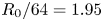 $R_0/64=1.95$ mm. Note that the AMR does not extend beyond
 $5R_0$ downstream to conserve computational resources, as well as to add numerical dissipation beyond the region of interest, thereby further mitigating numerical artefacts.
Two-dimensional slices of the density field for the full computational domain for two different simulations are provided in figure 1. This figure shows where grid resolution is added as well as the coarse grid beyond the near field that is intended to increase numerical dissipation prior to the boundary. Although we do not fully recover far-field scaling relationships within the relatively short region of maximum grid refinement, we do see velocity and density profiles approaching the Gaussian forms expected in the far field (Kaye & Hunt Reference Kaye and Hunt2009; Hunt & Van den Bremer Reference Hunt and Van den Bremer2011).
Two-dimensional slices through the entire computational domain of the density field for (a)  ${Ri}_0=2$,
 ${Re}_0=316$, and (b)
 ${Ri}_0=20$,
 ${Re}_0=316$. Half of the visualization corresponds to the density field
 $\rho$, and the other half visualizes the grid level
 $\ell$.

The bottom of the domain at  $z=0$ m is specified using Dirichlet boundary conditions with a hyperbolic tangent function, as proposed by Michalke (Reference Michalke1984) and used by others (Bharadwaj & Das Reference Bharadwaj and Das2017; Nichols et al. Reference Nichols, Schmid and Riley2007). Specifically, the profile is modelled using
 \begin{equation} \eta(x,y,0) = \frac{1}{2} - \frac{1}{2}\tanh \left[\frac{R_0}{4\phi}\left( \frac{R_0}{r} - \frac{r}{R_0} \right) \right], \end{equation}
where  $\phi = R_0/50=2.5\times 10^{-3}$ m is a smoothing factor that transitions the jet to the ambient, and
 $r \equiv (x^{2} + y^{2})^{1/2}$. The species mass fraction of helium and vertical velocity at the inlet are determined using
 $\eta$ by
 \begin{equation} Y_{He}(r,\theta,0) = \eta, \quad u_z(r,\theta,0) = \eta U_0, \end{equation}
where  $\theta =\tan ^{-1}(y/x)$ is the angle from the
 $x$-axis within the
 $x$–
 $y$ plane. From (2.4), the density can be inferred from the helium mass fraction field. Note that as
 $\phi \to 0$, this profile approaches a top-hat profile. The transverse velocity components are fixed at
 ${u_x = u_y = 0}$, mimicking a no-slip wall outside of the flow stream. The remaining five boundaries are open, with boundary velocities computed to satisfy (2.3), enabling the entrainment of ambient air from outside the domain or the outflow of helium–air mixture from within the domain.
2.4. Present simulations
To vary  ${Ri}_0$ and
 ${Re}_0$ independently in the simulations, we change only the magnitude of the gravitational acceleration
 $g$, and the inflow velocity
 $U_0$. All other parameters remain fixed for all simulations, and the complete set of dynamically relevant inlet parameters is given in table 1. Note that once the two fluids (i.e. helium and air in the present case) have been selected, we can change
 ${Ri}_0$ and
 ${Re}_0$ independently by modifying any two of the following three variables:
 $U_0$,
 $g$ and
 $R_0$. In the present study, we chose to modify only
 $U_0$ and
 $g$ since changes in
 $R_0$ would require us to also vary the smoothing factor
 $\phi$ and the domain size
 $L$ in order to keep
 $\phi /R_0$ and
 $L/R_0$ constant. A single value of species diffusivity is appropriate because diffusion must be equal and opposite for a binary fluid system.
List of all independent, dynamically relevant inlet parameters for the buoyant plume simulations. Parameters with numerical values are fixed for all simulations.

The complete set of non-dimensional groups based on the parameters in table 1 is given in table 2. Note that the Richardson number used here can be expressed as a combination of  ${Fr}_0$ and the density ratio
 $\tilde {\rho }$, as
 ${Ri}_0=(1-1/\tilde {\rho })\,{Fr}_0^{-2}$. This definition does not originate from dimensional analysis, and instead comes from the finding that the puffing frequency in terms of the Strouhal number is well correlated with this form of the Richardson number (as discussed in detail in Bharadwaj & Das Reference Bharadwaj and Das2017). Table 3 provides a summary of the different values of
 ${Ri}_0$ and
 ${Re}_0$ in the simulations, where each is obtained by varying only
 $g$ and
 $U_0$. In total, 18 simulations are performed, with
 ${Ri}_0$ and
 ${Re}_0$ each varying by at least an order of magnitude.
Non-dimensional numbers formed from the independent, dynamically relevant inlet parameters in table 1. Non-dimensional numbers with numerical values are fixed for all simulations.

Parameters of the simulations performed herein, with corresponding definitions given in tables 1 and 2. We also provide the domain side length ( $L/R_0$), the amount of data collected for each simulation (
 $T/\tau ^{*}$), and the time step between snapshots used for statistics (
 $\tau ^{*}/\Delta t$).

In figure 2 we show  ${Ri}_0$ and
 ${Re}_0$ for the present simulations compared to previous experiments of unsteady, axisymmetric helium jets and plumes (Subbarao & Cantwell Reference Subbarao and Cantwell1992; Kyle & Sreenivasan Reference Kyle and Sreenivasan1993; Cetegen & Kasper Reference Cetegen and Kasper1996; Cetegen Reference Cetegen1997a; Pasumarthi & Agrawal Reference Pasumarthi and Agrawal2003; Yep, Agrawal & Griffin Reference Yep, Agrawal and Griffin2003; O'Hern et al. Reference O'Hern, Weckman, Gerhart, Tieszen and Schefer2005; Hallberg & Strykowski Reference Hallberg and Strykowski2006; Bharadwaj & Das Reference Bharadwaj and Das2017). Note that Hamins, Yang & Kashiwagi (Reference Hamins, Yang and Kashiwagi1992) also performed experiments with this configuration, although we were unable to recover the Reynolds number for this study. Figure 2 shows that the present simulations correspond to values of
 ${Re}_0$ generally higher than in prior experiments. Since the inflow velocity
 $U_0$ is often varied in experiments to explore different conditions, the experimental studies in figure 2 follow approximate
 ${Ri}_0 \sim {Re}_0^{-2}$ scaling relations, where
 ${Ri}_0\sim U_0^{-2}$ and
 ${Re}_0\sim U_0$.
Richardson and Reynolds number values for previously conducted experiments of axisymmetric, unsteady helium jets and plumes, as well as the present simulations. The legend corresponds to the following references: B17 – Bharadwaj & Das (Reference Bharadwaj and Das2017); C96 – Cetegen & Kasper (Reference Cetegen and Kasper1996); C97 – Cetegen (Reference Cetegen1997a); H06 – Hallberg & Strykowski (Reference Hallberg and Strykowski2006); K93 – Kyle & Sreenivasan (Reference Kyle and Sreenivasan1993); O05 – O'Hern et al. (Reference O'Hern, Weckman, Gerhart, Tieszen and Schefer2005); P03 – Pasumarthi & Agrawal (Reference Pasumarthi and Agrawal2003); S92 – Subbarao & Cantwell (Reference Subbarao and Cantwell1992); and Y05 – Yep et al. (Reference Yep, Agrawal and Griffin2003). The red dashed line shows the approximate onset of the puffing instability as provided by Bharadwaj & Das (Reference Bharadwaj and Das2017).

Table 3 provides temporal information for the data collected during the simulations. To collect data that are sufficiently well-resolved temporally, we estimate an expected eddy turnover time  $\tau ^{*}\equiv 1/f^{*}$, where
 $f^{*}$ denotes the predicted puffing frequency based on
 ${Ri}_0$ and (1.1). Using this estimate of
 $\tau ^{*}$, we first let each simulation spin-up for approximately
 $20\tau ^{*}$ to allow initial transients to decay. We then collect data for
 $T \approx 100\tau ^{*}$ with output interval
 $\Delta t \approx \tau ^{*}/40$, both of which are sufficient to temporally resolve large-scale flow phenomena as well as provide statistically converged results for moments of many different flow variables.
3. Results and discussion
3.1. Qualitative plume structure and dynamics
The qualitative plume structure and dynamics are indicated in figure 3, which shows time series of the density field over a time span of roughly  $\tau ^{*}$ for two different values of
 ${Ri}_0$, as well as three different values of
 ${Re}_0$ for each
 ${Ri}_0$. Note that
 $\tau ^{*}$ generally decreases with increasing
 ${Ri}_0$ and increasing
 ${Re}_0$, and therefore the time series in figure 3 span different physical times.
Time series of the density field over a time span of roughly  $\tau ^{*}$ for six different cases: (a)
 ${Ri}_0=2$,
 ${Re}_0=100$; (b)
 ${Ri}_0=2$,
 ${Re}_0=316$; (c)
 ${Ri}_0=2$,
 ${Re}_0=1000$; (d)
 ${Ri}_0=20$,
 ${Re}_0=100$; (e)
 ${Ri}_0=20$,
 ${Re}_0=316$; (f)
 ${Ri}_0=20$,
 ${Re}_0=1000$. Time progresses in increments of
 $\tau ^{*}/4$ from left to right. Panels (a i–f i) show where the AMR grid is refined, with grey indicating
 $\ell =2$, and black indicating
 $\ell =3$. Panels (a v–f v) include the in-plane direction of the velocity vector (not scaled with velocity magnitude).

In each of the simulations, figure 3 shows that large-scale vortical structures form at the base of the plume and then rise vertically due to buoyancy, entraining fluid as they propagate (this entrainment is indicated by the streamlines provided in the rightmost column of the figure). This process repeats for the duration of the simulations at a time scale of approximately  $\tau ^{*}$, corresponding to the puffing instability discussed in § 1; measurements of
 $\tau ^{*}$ and the puffing frequency are given in § 3.5. Figure 3 further shows that the vortical structures are more diffuse for the
 ${Ri}_0=2$,
 ${Re}_0=100$ case, as compared to larger values of
 ${Re}_0$ at the same
 ${Ri}_0$. This is due to the slower propagation speed of the vortices, as compared to the rate of diffusion.
From a dynamical perspective, figure 3 shows that at  ${Ri}_0=2$,
 ${Re}_0=1000$, the puffing oscillations undergo a transition where the vortices become more turbulent, as indicated by the development of motions over multiple scales within the vortices, consistent with experimental observations made by Subbarao & Cantwell (Reference Subbarao and Cantwell1992). The plume also appears to lean to one side as a result of a flapping mode, which has been observed previously in both non-reacting plumes (Cetegen Reference Cetegen1997b) and diffusion flames Cetegen & Dong (Reference Cetegen and Dong2000); this mode will be discussed in more detail in § 3.2.
For the  ${Ri}_0=20$,
 ${Re}_0=100$ case shown in figure 3, there is still relatively little small-scale motion due to the low
 ${Re}_0$, but the formation of vortices is more sinuous (i.e. anti-symmetric) in nature, as compared to the varicose (i.e. symmetric) behaviour observed at the same
 ${Re}_0$ for
 ${Ri}_0=2$. At larger
 ${Re}_0$ for
 ${Ri}_0=20$, the flow is generally turbulent, even along the centreline near the bottom of the domain. This early transition to turbulence is correlated with the penetration of heavy air into the core of the plume, as can be seen in a number of snapshots. We call these Rayleigh–Taylor (RT) spikes due to their resemblance to classical RT instabilities. Overall, this leads to a puffing instability that is more turbulent than the puffing instability at lower
 ${Ri}_0$ and
 ${Re}_0$.
3.2. Temporal variability
Figure 4 shows time series of the vertical velocity  $u_z/U_0$ and
 $Y_{He}$ at height
 $z/R_0=0.5$ along the centreline (i.e.
 $r/R_0=0$) over time span
 $10\tau ^{*}$. Note that time in figure 4 has been normalized by the expected time scale
 $\tau ^{*}$, based on (1.1) rather than on the computed puffing frequency, which is presented and discussed in § 3.5. In general, the time series of
 $u_z/U_0$ become increasingly complex with increasing
 ${Ri}_0$ and
 ${Re}_0$. For
 ${Ri}_0=2$ in figure 4(a), the time series are smooth and periodic for all
 ${Re}_0$, with a characteristic time scale close to
 $\tau ^{*}$, corresponding to the puffing motion. As either
 ${Ri}_0$ or
 ${Re}_0$ is increased, the local minima and maxima begin to vary more substantially from cycle to cycle. For sufficiently high
 ${Re}_0$, the signals become erratic and chaotic, indicating the transition to a fully turbulent plume as shown, for instance, in figures 4(c,d).
Time series of (a–d)  $u_z/U_0$ and (e–h)
 $Y_{He}$ on the centreline (
 $r/R_0=0$) at height
 $z/R_0=0.5$ above the plume. Different line colours and widths correspond to different values of
 ${Re}_0$. Note that the time has been normalized by the expected time scale
 $\tau ^{*}$, based on (1.1) rather than the computed puffing frequency presented later in the text. Plots are for: (a,e)
 ${Ri}_0 = 2$, (b,f)
 ${Ri}_0 = 6.3$, (c,g)
 ${Ri}_0 = 20$, and (d,h)
 ${Ri}_0 = 63$.

Significantly, the transition to turbulent behaviour does not occur monotonically with increasing  ${Re}_0$. For
 ${Ri}_0=2$ in figure 4(a), the local maxima in
 $u_z/U_0$ are much more consistent between each puffing cycle for
 ${Re}_0=100$ and
 ${Re}_0=1000$, while at
 ${Re}_0=316$, the local maxima between each puffing cycle vary more substantially. This increasing complexity is also evident in the time series of
 $Y_{He}$ for
 ${Ri}_0=6.3$ shown in figure 4(f); the only deviation from a uniform time series occurs momentarily for the intermediate Reynolds number
 ${Re}_0=316$. This behaviour is more consistent with nonlinear dynamical systems that have complex paths to chaos (e.g. period doubling phenomena, windows of less chaotic dynamics) rather than a simple broadening of scales typical of a fully turbulent flow.
The effects of the RT spikes noted in figure 3 are also evident in figure 4. For the two smallest values of  ${Ri}_0$, in figures 4(e,f),
 $Y_{He}\approx 1$ at all times, implying that the more dense ambient air does not penetrate the centre of the plume at
 $z/R_0 = 0.5$. However, for
 ${Ri}_0=20$ and
 $63$ in figures 4(g,h),
 $Y_{He}$ frequently decreases below
 $1$, with the frequency, duration and strength of the decreases growing as
 ${Ri}_0$ and
 ${Re}_0$ increase. As indicated in figure 3, instances of
 $Y_{He} < 1$ are not a result of shear layer roll-up causing the ambient air to reach the centreline horizontally. Rather, these decreases are a result of a downward spike of heavier air. This phenomenon is particularly important when considering extensions to reacting plumes, since this would indicate the presence of an additional mechanism for supplying oxidizer to the flame beyond the mixing along the shear layer.
The flapping motion mentioned in § 3.1 and shown for the  ${Ri}_0=2$,
 ${Re}_0=1000$ case in figure 3 is indicated quantitatively in figure 5 through time series of the radial velocity
 $u_r/U_0$ on the plume centreline at
 $z/R_0=0.5$. The radial velocity, in particular, corresponds to horizontal motions of the plume in the
 $x$–
 $y$ plane and is thus associated with the horizontal flapping behaviour shown in figure 3. For
 ${Ri}_0=2$ and
 ${Re}_0=1000$ in figure 5(a),
 $u_r/U_0$ oscillates at a frequency that is half that of the oscillations in
 $u_z/U_0$ shown in figure 4(a), although both oscillations are synchronized. That is, despite the difference in frequency, the sinuous mode associated with the plume flapping is synchronized with the varicose mode associated with the puffing. The flapping oscillation does not occur for the smaller values of
 ${Re}_0$ at
 ${Ri}_0=2$, although figure 5(b) shows that the oscillation occurs for all
 ${Re}_0$ at
 ${Ri}_0=6.3$. Variations in the radial velocity in the more turbulent simulations for higher
 ${Ri}_0$ are due primarily to the turbulent nature of the flow, rather than to a distinguishable oscillatory mode, hence we do not plot them here.
Time series of  $u_r/U_0$ on the centreline (
 $r/R_0=0$) at height
 $z/R_0=0.5$ above the plume for (a)
 ${Ri}_0=2$ and (b)
 ${Ri}_0=6.3$. Different line colours and widths correspond to different values of
 ${Re}_0$.

The dynamics in the shear layer are indicated by the time series of  $u_z/U_0$ and
 $Y_{He}$ shown in figure 6. These time series are taken at the same height (i.e.
 $z/R_0=0.5$) as in figure 4, but at radial location
 $r=\delta _Y/2$, where
 $\delta _Y/2$ is the half-width of the flow based on where the temporal and azimuthal average of
 $Y_{He}$ is 0.5. By probing this radial location, we ensure that there are substantial and coherent fluctuations in the density field for all simulations, unlike at the centreline.
Same as figure 4, but at location  $r=\delta _Y/2$,
 $z/R_0=0.5$ within the shear layer.

The time series of  $u_z/U_0$ in figures 6(a–d) are generally consistent with the centreline results in figure 4. Namely, the complexity of the time series increases with increasing
 ${Ri}_0$ and
 ${Re}_0$, with consistently repeating signals observed only for the smallest value of
 ${Ri}_0$ shown in figure 6(a). By contrast to the centreline results, however, the increase in complexity occurs monotonically for each
 ${Ri}_0$ with increasing
 ${Re}_0$; these trends will be discussed in more detail in § 3.3.
The shear layer time series of  $Y_{He}$ in figures 6(e–h) vary far more substantially at each value of
 ${Ri}_0$ and
 ${Re}_0$ than the corresponding centreline time series in figure 4. Most notably, for
 ${Ri}_0=2$ as
 ${Re}_0$ increases, figure 6(e) shows a transition from a smooth, almost sinusoidal, variation in
 $Y_{He}$ to a time series with more distinct plateaus at
 $Y_{He}\approx 1$. This is the result of the slower time scale associated with convection for the lower
 ${Re}_0$, allowing for increased broadening of the helium–air interface as a result of diffusion. At larger
 ${Re}_0$, the flow is accelerated more rapidly, and as a result, can produce gradients that are even stronger than those initiated at the inlet. This transition can also be seen at
 ${Ri}_0=6.3$ in figure 6(f) for lower
 ${Re}_0$. In the simulations with
 ${Ri}_0\geq 20$, while the signals are not as regular, we also see sharper changes in
 $Y_{He}$ within the shear layer, as compared with the centreline results in figure 4, consistent with previous observations of scalar mixing in turbulent flows (Sandoval Reference Sandoval1995; Buch & Dahm Reference Buch and Dahm1998).
Finally, at the location in the shear layer, there are clear and consistent phase relationships between the different variables. Because density (related directly to  $Y_{He}$) is an active scalar for vertical momentum transport, it is intuitive that local changes in
 $Y_{He}$ would also be reflected in
 $u_z$. In particular, comparison of figures 6(a–d) with figures 6(e–h) reveals that large peaks in
 $u_z/U_0$ are preceded by increases in
 $Y_{He}$. This makes sense intuitively because larger density discrepancies lead to larger buoyant forces that accelerate the flow. This is true for both the laminar and turbulent plumes, and these correlations are examined in more detail in the next subsection.
3.3. Transition from laminar to turbulent flow
A transition from laminar to chaotic dynamics in the near field of the plumes can be observed in the time series in § 3.2 as  ${Ri}_0$ and
 ${Re}_0$ increase. In this subsection, we examine this transition more closely by using the state space dynamics of the vertical velocity
 $u_z/U_0$. We first focus on this transition in the near-field region where the puffing instability is most evident. It is important to note that for buoyant plumes, the flow will transition from laminar to turbulent sufficiently far downstream (except for very small
 ${Re}_0$), since potential energy is continually converted to kinetic energy, resulting in an increase in the local Reynolds number (Hunt & Van den Bremer Reference Hunt and Van den Bremer2011). Therefore, we first focus on this transition at a fixed spatial location within the near-field region, then show the transition from laminar to chaotic dynamics as downstream distance is varied.
To begin, figure 7 shows the state space of  $u_z(t+\tau ^{*}/4)/U_0$ versus
 $u_z(t)/U_0$ along the centreline at
 $z/R_0=0.5$ for each simulation summarized in table 3. Each trajectory is coloured according to the simulation time such that lighter yellow indicates earlier times and darker blue indicates later times. White space indicates a state that the trajectory does not reach for the given spatial location during the analysis period. For the two smallest values of
 ${Re}_0$ in the
 ${Ri}_0=2$ and
 $6.3$ cases, the state-space trajectories form a stable limit cycle corresponding to the puffing behaviour. However, as
 ${Re}_0$ increases to
 $316$ for
 ${Ri}_0=2$, the trajectory is not as consistent compared to other trajectories for this value of
 ${Ri}_0$, even compared to higher
 ${Re}_0$, indicating increased flow complexity. This ‘island’ of increased variability, as indicated by the larger amount of state space occupied by the trajectory, is consistent with the non-monotonicity with
 ${Re}_0$ noted in figure 4(a), and is likely due to the complex coupling between the puffing oscillations and shear layer roll up. Overall, however, for
 ${Ri}_0=2$, figure 7 does not reveal a transition to fully chaotic (i.e. turbulent) dynamics for the range of
 ${Re}_0$ examined here.
State-space trajectories of the vertical velocity at  $r/R_0=0$,
 $z/R_0=0.5$, generated by plotting the same signal on different axes with an offset by
 $\tau ^{*}/4$. The lines are coloured by time elapsed during the simulation. Plots are for: (a–e)
 $Ri_0 = 2$, (f–j)
 $Ri_0 = 6.3$, (k–o)
 $Ri_0 = 20$, (p–r)
 $Ri_0 = 63$; and (a,f,k,p)
 $Re_0=100$, (b,g,l,q)
 $Re_0=178$, (c,h,m,r)
 $Re_0=316$, (d,i,n)
 $Re_0=562$, (e,j,o)
 $Re_0=1000$.

For  ${Ri}_0=6.3$, by contrast, figure 7(f–j) shows that there is a substantial increase in complexity between
 ${Re}_0=178$ and
 ${Re}_0=316$. Because
 ${Re}_0$ controls the prevalence of small-scale motions and the onset of nonlinear chaotic dynamics, after a critical
 ${Re}_0$, the puffing instability becomes sufficiently chaotic such that the state-space trajectories are not as consistent. When this occurs, the trajectories occupy more of the state-space locations within a bounded region, eventually exploring most points within the region. Additional data and analysis are required to claim definitively whether the trajectories occupy all of the state space within the bounded region. For the two highest values of
 ${Ri}_0$ examined here, figure 7 shows that the state-space dynamics are fully chaotic even for the lowest
 ${Re}_0$, indicating that the transition to chaotic dynamics in these cases occurs for
 ${Re}_0$ less than 100.
Based on these results, the critical Reynolds number, denoted  ${Re}_{crit}$, at which the transition to chaotic dynamics occurs depends on
 ${Ri}_0$, with smaller values of
 ${Re}_{crit}$ for increasing
 ${Ri}_0$. Among the present simulations,
 ${Re}_{crit}>1000$ for
 ${Ri}_0=2$,
 $178<{Re}_{crit}<316$ for
 ${Ri}_0=6.3$, and
 ${Re}_{crit}<100$ for both
 ${Ri}_0=20$ and
 $63$. In general, for a given
 ${Ri}_0$, as
 ${Re}_0$ increases, the flow transitions from steady laminar to unsteady laminar, to unsteady transitional, to unsteady turbulent behaviours.
The state-space trajectories in figure 7 are all calculated at a single centreline location, but the transition from laminar to turbulent behaviours also occurs with increasing vertical location due to the conversion of potential (i.e. buoyant) energy into kinetic energy. Figure 8 shows this transition for the  ${Ri}_0=2$,
 ${Re}_0=1000$ case. At
 $z/R_0=0.25$ and
 $1$, the state-space trajectories approximately follow stable limit cycles, but at
 $z/R_0=2$, the region of state space occupied by the trajectory has grown substantially and the trajectory explores essentially all of the states within this region.
State-space trajectories of the vertical velocity for  ${Ri}_0=2$,
 ${Re}_0=1000$ along the centreline at different vertical locations. The lines are coloured the same as in figure 7: (a)
 $z/R_0=0.25$, (b)
 $z/R_0=1$, (c)
 $z/R_0=2$.

This dynamical transition with downstream location is expected in most plumes as the flow convects vertically (Hunt & Van den Bremer Reference Hunt and Van den Bremer2011) and has been noted before by Subbarao & Cantwell (Reference Subbarao and Cantwell1992). It is possible that a robust criterion could be derived to show more precisely the spatial location where this transition occurs. For example, estimates of the correlation dimension can be computed using standard algorithms in nonlinear dynamics (Hegger, Kantz & Schreiber Reference Hegger, Kantz and Schreiber1999), where most laminar cases would be essentially one-dimensional but turbulent ones would be larger; this analysis has been done for the closely related flame flickering instability (Gotoda, Kawaguchi & Saso Reference Gotoda, Kawaguchi and Saso2008). Application of these criteria to the present simulations is left as a direction for future research.
It should be noted that within the two distinct regimes of puffing indicated by figures 7 and 8 (i.e. laminar and turbulent), the state-space trajectories continue to change with increasing  ${Re}_0$. For example, in the
 ${Ri}_0=2$ simulations at the two lowest values of
 ${Re}_0$, we see ‘period doubling’ behaviour where the periodic trajectory changes from requiring one orbit at
 ${Re}_0=100$ to two orbits at
 ${Re}_0=178$ to return to the same state-space location. For the two highest values of
 ${Ri}_0$, the flow is turbulent for all
 ${Re}_0$, but the bounded region within which the state-space trajectories reside grows with increasing
 ${Re}_0$. This is consistent with many turbulent flows where increases in the Reynolds number correspond to an increasing prevalence of intermittent rare events that expand the occupied state-space region. At a certain value of
 ${Re}_0$, however, results for the two largest values of
 ${Ri}_0$ shown in figure 8 indicate that this region approaches a fixed size, corresponding to fully turbulent behaviour.
3.4. Temporal correlations
The results in § 3.2 suggest that the flow variables are correlated in potentially complicated ways. These correlations and the temporal correspondence between variables can be examined in more detail using state-space trajectories such as those shown in figure 9, where trajectories are calculated in the  $p$–
 $u_z$ state space along the centreline at
 $z/R_0=0.5$ for three different values of
 ${Re}_0$ and for each
 ${Ri}_0$. For
 ${Ri}_0=2$ and
 ${Re}_0=100$,
 $p$ and
 $u_z$ are highly correlated, with
 $p$ lagging behind
 $u_z$ (i.e. the trajectory in figure 9(a) goes counterclockwise as time evolves). In the context of these state-space trajectories, correlations are indicated by consistent orbital motions through state space, where
 $p$ and
 $u_z$ vary together in a regular way.
State-space trajectories of the vertical velocity  $u_z/U_0$ and mechanical pressure
 $p/\rho _\infty U_0^{2}$ at
 $r/R_0=0$,
 $z/R_0=0.5$. The lines are coloured by time elapsed during the simulation. Plots are for: (a)
 $Ri_0=2$,
 $Re_0=100$; (b)
 $Ri_0=6.3$,
 $Re_0=100$; (c)
 $Ri_0=20$,
 $Re_0=100$; (d)
 $Ri_0=63$,
 $Re_0=100$; (e)
 $Ri_0=2$,
 $Re_0=316$; (f)
 $Ri_0=6.3$,
 $Re_0=316$; (g)
 $Ri_0=20$,
 $Re_0=316$; (h)
 $Ri_0=63$,
 $Re_0=316$; (i)
 $Ri_0=2$,
 $Re_0=1000$; (j)
 $Ri_0=6.3$,
 $Re_0=1000$; (k)
 $Ri_0=20$,
 $Re_0=1000$.

As  ${Ri}_0$ increases from 2 to 6.3, figure 9(b) shows that the state-space trajectories become more complex, with period doubling and slight broadening of the limit cycles, although
 $p$ still lags behind
 $u_z$. Further increases in
 ${Re}_0$ or
 ${Ri}_0$ result in a chaotic flow for which the correlation between
 $p$ and
 $u_z$ is much less pronounced. In particular, results for the larger values of
 ${Re}_0$ and
 ${Ri}_0$ in figure 9 show that some orbital trajectories do still exist, but the trajectories explore an increasingly large region of state space. State-space trajectories including
 $u_r$ and
 $Y_{He}$ are less interesting at this spatial location and are thus not shown here.
Figure 10 shows corresponding state-space trajectories within the shear layer at  $z/R_0=0.5$,
 $r=\delta _Y/2$. Given the more substantial variations in
 $u_r$ and
 $Y_{He}$ at this location (as is also indicated by the variations in figure 6), here we show state-space trajectories for all possible combinations of
 $Y_{He}$,
 $u_r$ and
 $p$. Once again, for small
 ${Ri}_0$ and
 ${Re}_0$, these trajectories form closed and compact orbits, with
 $u_r$ and
 $Y_{He}$ lagging behind
 $p$. Large values of
 $u_r$ and
 $Y_{He}$ are generally highly correlated since, when
 $u_r$ is large and positive (i.e. the plume is not entraining strongly), the flow is generally accelerated vertically by buoyancy, corresponding to higher values of
 $Y_{He}$.
Correlations between  $Y_{He}$ and
 $u_r$ (green circles),
 $Y_{He}$ and
 $p$ (blue squares), and
 $u_r$ and
 $p$ (red triangles), at
 $r=\delta _Y/2$,
 $z/R_0=0.5$ within the shear layer for several of the simulations. Plots are for: (a)
 $Ri_0=2$,
 $Re_0=100$; (b)
 $Ri_0=6.3$,
 $Re_0=100$; (c)
 $Ri_0=20$,
 $Re_0=100$; (d)
 $Ri_0=63$,
 $Re_0=100$; (e)
 $Ri_0=2$,
 $Re_0=316$; (f)
 $Ri_0=6.3$,
 $Re_0=316$; (g)
 $Ri_0=20$,
 $Re_0=316$; (h)
 $Ri_0=63$,
 $Re_0=316$; (i)
 $Ri_0=2$,
 $Re_0=1000$; (j)
 $Ri_0=6.3$,
 $Re_0=1000$; (k)
 $Ri_0=20$,
 $Re_0=1000$.

3.5. Puffing frequency
The frequency at which large-scale vortices are shed during the buoyant plume evolution is commonly referred to as the puffing frequency. This frequency is the most widely used statistical measure of the puffing instability, and both experimental and computational approaches can easily measure and compare this simple metric. In our simulations, the periodic puffing motion is present qualitatively in essentially all the data presented in §§ 3.1–3.4.
The most typical and simplest method of measuring the puffing frequency is to extract a time series of a flow variable (typically the mechanical pressure or vertical velocity) and perform a fast Fourier transform (FFT) to obtain the power spectral density (PSD) of the signal. The peak of the PSD is generally classified as the puffing frequency. In figure 11, we show the PSD of the vertical velocity  $u_z$ taken along the centreline at
 $z/R_0=0.5$ for six different simulations. Each of the PSDs has been normalized by the maximum magnitude, and the Strouhal number
 ${St}_0$ is normalized by the expected value
 ${St}_0^{*}$ based on Wimer et al. (Reference Wimer, Lapointe, Christopher, Nigam, Hayden, Upadhye, Strobel, Rieker and Hamlington2020) and (1.1).
Normalized power spectral densities (PSDs) of  $u_z$ along the centreline at
 $z/R_0 = 0.5$ for (a–c)
 ${Ri}_0=2$ and (d–f)
 ${Ri}_0=20$, at (a,d)
 ${Re}_0=100$, (b,e)
 ${Re}_0=316$, and (c,f)
 ${Re}_0=1000$. The observed Strouhal number
 ${St}_0$ is normalized by the predicted value
 ${St}^{*}_0$ obtained from (1.1).

For  ${Ri}_0=2$ and all values of
 ${Re}_0$, figures 11(a–c) show that each PSD has a distinct peak at
 ${St}_0/{St}_0^{*} \approx 0.84$, indicating that the puffing frequency is slightly below that predicted by Wimer et al. (Reference Wimer, Lapointe, Christopher, Nigam, Hayden, Upadhye, Strobel, Rieker and Hamlington2020) (there are also smaller peaks at higher harmonics of the puffing frequency). For each of the
 ${Ri}_0=20$ cases, by contrast, we do not observe as clear a peak in the PSD. When
 ${Re}_0=100$ in figure 11(d), there are actually two peaks that could conceivably be identified as the puffing frequency. At
 ${Re}_0=316$ in figure 11(e), the peak in the signal is fairly clear but far from the expected value. At
 ${Re}_0=1000$ in figure 11(f), it is difficult to say with any certainty that a single distinct peak even exists.
Given the results in figure 11, measuring a single distinct puffing frequency for each simulation using a probing technique can be difficult. Subbarao & Cantwell (Reference Subbarao and Cantwell1992) also noted this difficulty for higher  ${Re}$ flows when conducting experiments. Because puffing is a global instability, we should be able, in principle, to probe the flow anywhere within the plume and determine the puffing frequency. In previous studies, the probe location was typically placed where the largest fluctuations occur, roughly one radius vertically along the centreline (Cetegen & Kasper Reference Cetegen and Kasper1996) or slightly off-centre at the base of the plume (Bharadwaj & Das Reference Bharadwaj and Das2017). A more robust technique that better captures the global nature of the instability was used by Wimer et al. (Reference Wimer, Day, Lapointe, Meehan, Makowiecki, Glusman, Daily, Rieker and Hamlington2021), where a singular value decomposition (SVD) was performed on two-dimensional slices of vertical velocity.
For the present simulations, neither a single probe nor an SVD approach produced consistent results that reflected accurately the puffing frequency for all simulations. The complexity of measuring the puffing frequency is indicated in figure 12. At each spatial location, we computed the FFT of the time series of vertical velocity, identified which frequency was associated with the peak in the spectra, computed  ${St}_0$ corresponding to that frequency, then normalized based on the expected
 ${St}_0^{*}$ from (1.1). This was done for each simulation, and one radial slice is shown in figure 12. Further, we used a binary logarithm,
 $\log _2({St}_0/{St}_0^{*})$, such that a value of 0 (white in figure 12) corresponds to the peak
 ${St}_0$ being identical to
 $St_0^{*}$, and integer values correspond to harmonics of
 ${St}_0^{*}$.
Frequency corresponding to the peak in the PSD of the fluctuating streamwise velocity computed at each spatial location within a radial slice for all simulations performed in this study. Images are coloured using 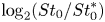 $\log _2({St}_0/{St}_0^{*})$ such that 0 (or white) corresponds to the computed
 ${St}_0$ being identical to
 ${St}_0^{*}$ from (1.1), with integer values corresponding to harmonics. Plots are for (a–e)
 $Ri_0 = 2$, (f–j)
 $Ri_0 = 6.3$, (k–o)
 $Ri_0 = 20$, (p,q,r)
 $Ri_0 = 63$, with (a,f,k,p)
 $Re_0=100$, (b,g,l,q)
 $Re_0=178$, (c,h,m,r)
 $Re_0=316$, (d,i,n)
 $Re_0=562$, (e,j,o)
 $Re_0=1000$.

At  ${Ri}_0=2$ in figure 12, almost the entire
 $r$–
 $z$ plane shows a consistent puffing frequency that is slightly below the expected value
 ${St}_0^{*}$. This is perhaps not surprising given that in figure 3, the flow is laminar for
 $z<1.5R_0$. The regions of dark blue and red are harmonics of
 ${St}_0$. At
 ${Ri}_0=6.3$, the region
 ${St}_0 \lesssim {St}_0^{*}$ becomes more confined for increasing
 ${Re}_0$, with values of
 ${St}_0$ tending towards
 $St_0^{*}$ as
 ${Re}_0$ increases. A similar variation with
 ${Re}_0$ is observed for
 ${Ri}_0=20$, except that in this case
 ${St}_0$ increases above
 ${St}_0^{*}$, most notably for
 ${Re}_0=316$ and
 ${Re}_0=562$. For
 ${Re}_0=100$ and
 ${Re}_0=178$ at
 ${Ri}_0=62$, the region that is close to
 ${St}_0^{*}$ is very small, even though the flow fields in figure 3 indicate the presence of pulsatile flow.
It is interesting to note that figure 12 shows that a low-frequency region forms near the centreline at the base of the plume for  ${Ri}_0=20$,
 ${Re}_0\geq 178$, and for all simulations at
 ${Ri}_0=63$. Connecting this back to figure 4, these are also the simulations where RT spikes form along the centreline. Because these spikes cause large fluctuations in the vertical velocity on a time scale much larger than the puffing instability, the computed
 ${St}_0$ in this area is much smaller than the
 ${St}_0$ associated with the puffing.
To determine quantitatively the puffing frequency dependence on  ${Ri}_0$ and
 ${Re}_0$, we apply the probe technique to the 3-D volume
 $x\in [-2R_0,2R_0]$,
 $y\in [-2R_0,2R_0]$ and
 $z\in [0,5R_0]$, resulting in fields of peak frequencies similar to those shown in figure 12. If the frequency at a particular spatial location satisfies
 $|{\log _2({St}_0/{St}_0^{*})}| < \log _2(4/3)$, then this frequency is retained for further analysis. This bound was chosen because the puffing frequency must fall within this range based on many previous measurements (Wimer et al. Reference Wimer, Lapointe, Christopher, Nigam, Hayden, Upadhye, Strobel, Rieker and Hamlington2020), and if a computed frequency falls outside this range, then it is most likely not associated with the puffing instability. Among the spatial locations that fall within this range, the most common value of
 ${St}_0$ (i.e. the mode) is shown in figure 13 for all simulations.
Puffing frequency measured by the most commonly computed  ${St}_0$ value in each simulation. Symbols correspond to different
 ${Ri}_0$, and colours correspond to different
 ${Re}_0$. (a) Puffing frequency as a function of
 ${Ri}_0$. (b) Puffing frequency as a function of
 ${Re}_0$. The dashed lines are the empirical correlation predicted by Wimer et al. (Reference Wimer, Lapointe, Christopher, Nigam, Hayden, Upadhye, Strobel, Rieker and Hamlington2020) and indicated in (1.1).

Figure 13(a) shows that the strongest variations in  ${St}_0$ occur with changes in
 ${Ri}_0$. In particular,
 ${St}_0$ increases with increasing
 ${Ri}_0$, and the dependence on
 ${Re}_0$ is relatively weak. As
 ${Ri}_0$ increases, there is an increase in
 ${St}_0$ relative to the scaling proposed in (1.1). Nevertheless, the present results do lie close to this relationship, which was proposed in Wimer et al. (Reference Wimer, Lapointe, Christopher, Nigam, Hayden, Upadhye, Strobel, Rieker and Hamlington2020) based on a wide range of data sources.
Although the dependence of  ${St}_0$ on
 ${Re}_0$ is not as strong as the dependence on
 ${Ri}_0$, figure 13(b) does reveal that there are variations in
 ${St}_0$ with
 ${Re}_0$. For the two highest values of
 ${Ri}_0$, in particular, figure 13(b) shows that
 ${St}_0$ reaches a maximum value at an intermediate value of
 ${Re}_0$ (316 in the case
 ${Ri}_0=20$, and 178 for
 ${Ri}_0=63$), but decreases for both smaller and larger values of
 ${Re}_0$. The dependence of
 ${St}_0$ on
 ${Re}_0$ is less pronounced for the two smaller values of
 ${Ri}_0$,
Based on the spatially varying puffing frequency fields shown in figure 12, there are several points to note regarding the single values of the puffing frequency shown in figure 13. First, as  ${Ri}_0$ increases, figure 12 shows that the spatial region where the probe can be used to measure the puffing frequency narrows substantially. Additionally, within this region, there is also some uncertainty in the precise value of the puffing frequency. For example, at
 ${Ri}_0=20$ and
 ${Re}_0=1000$, as well as at
 ${Ri}_0=63$ and
 ${Re}_0=316$, there are different peak frequencies all within the same spatial region; any of these frequencies could be associated reasonably with the puffing frequency. These variations indicate greater uncertainty in the measurement of a single global puffing frequency associated with the plume dynamics.
Taken together, figures 12 and 13 suggest the following dependence of the puffing frequency on  ${Ri}_0$ and
 ${Re}_0$. At low
 ${Re}_0$, the puffing frequency is consistently predicted below the scaling proposed in (1.1). As
 ${Re}_0$ increases, there is more uncertainty in the computed
 ${St}_0$, but the estimated
 ${St}_0$ approaches the proposed scaling. This trend is most clear for
 ${Ri}_0=20$: for
 ${Re}_0=100\unicode{x2013}178$,
 ${St}_0$ is below the proposed scaling; for
 ${Re}_0=316\unicode{x2013}562$,
 ${St}_0$ is above the scaling; and at
 ${Re}_0=1000$, the most commonly computed
 ${St}_0$ is near the proposed scaling, although with some uncertainty (based on the variability shown in figure 12).
Finally, it should be noted that the slight dependence of the puffing frequency on  ${Re}_0$ observed here does not contradict previous works (Subbarao & Cantwell Reference Subbarao and Cantwell1992; Bharadwaj & Das Reference Bharadwaj and Das2017), where a dependence on
 ${Re}_0$ has been neglected or was not observed. Based on our simulations, we start to see the increase in
 ${St}_0$ with
 ${Re}_0$ roughly where the flow transitions from laminar to turbulent, implying that this transitional regime induces a Reynolds number dependence. Additionally, it was shown experimentally by Cetegen & Kasper (Reference Cetegen and Kasper1996) that there is a change in the scaling of
 ${St}_0$ at high Richardson numbers. However, these high
 ${Ri}_0$ values were achieved by varying the inlet velocity
 $U_0$, thus
 ${Re}_0$ was varying simultaneously. From our analysis of the data presented in figure 13, if the critical
 ${Re}_0$ at which transition occurs continues to decrease with increasing
 ${Ri}_0$, then we expect that the data shown in Cetegen & Kasper (Reference Cetegen and Kasper1996) would be near this critical regime where the frequency was found here to be dependent upon
 ${Ri}_0$. Of course, in order to make the connection precise, many more simulations with different
 ${Ri}_0$ and
 ${Re}_0$ would need to be conducted, but this Reynolds number dependence offers a possible explanation for the change in scaling observed previously at large
 ${Ri}_0$.
4. Conclusions
A series of high-fidelity numerical simulations with AMR has been performed to model the injection of helium into quiescent air. In this study, we have focused specifically on how the inlet Richardson ( ${Ri}_0$) and Reynolds (
 ${Re}_0$) numbers impact the near-field temporal variability associated with the puffing instability as the flow transitions from laminar to turbulent. We report a number of new phenomena related to how the puffing instability transitions.
(i) As summarized in table 4, there are three distinct regimes of puffing: laminar, transitional and turbulent. The point of transition varies with spatial location,
 ${Ri}_0$ and ${Re}_0$. At a fixed spatial location, the critical ${Re}_0$ where these transitions occur decreases with increasing ${Ri}_0$. This increase in dynamical complexity is seen most easily using self-correlations of the vertical velocity along the centreline in the very near field.
(ii) Within the laminar puffing regime, we still observe qualitative changes in the puffing as
${Ri}_0$ and ${Re}_0$ vary. In particular, there is ‘period doubling’ where two cycles of the puffing motion are needed (as opposed to one cycle) for the flow to return to essentially the same state. A flapping mode is apparent, as indicated by strong coherent fluctuations of the radial velocity along the centreline, with some plumes showing intermittent flapping and others showing persistent flapping.(iii) In the transitional regime, the cycle-to-cycle variability in the puffing instability becomes chaotic, as indicated by the state-space trajectories. The flow, however, has not transitioned completely to fully turbulent since we do not observe penetration of heavy air into the core of the plumes, a feature that we call ‘spikes’ due to their resemblance to classical RT instabilities.
(iv) In the turbulent regime, we find RT spikes, and the consequences of these spikes are additional mixing and strong intermittent oscillations along the centreline of the plume, making the puffing frequency difficult to extract. The implications of this for reacting plumes would be the additional supply of oxidizer to the fuel. Additionally, within the turbulent puffing regime, the plumes exhibit a simple broadening of scales consistent with our view of turbulent homogeneous flows.
(v) Different flow variables are found to be almost perfectly correlated in the laminar regime, but in the turbulent regime, correlations are found related to only extreme events. As an example for
${Ri}_0=20$ where the flow is turbulent, decreases in mechanical pressure lead to rapid acceleration along the centreline. However, the correlations in general do not reflect simple dynamics (i.e. not a simple harmonic oscillator) and can vary spatially. This detail is important for models that propose different waveforms and phases of the variables (O'Hern et al. Reference O'Hern, Weckman, Gerhart, Tieszen and Schefer2005).(vi) The puffing frequency is found to be dependent on
${Re}_0$. Relative to the scaling relation proposed in Wimer et al. (Reference Wimer, Lapointe, Christopher, Nigam, Hayden, Upadhye, Strobel, Rieker and Hamlington2020) and shown in (1.1), the puffing frequency is initially below the expected ${St}_0$ for sufficiently low ${Re}_0$ and ${Ri}_0$; then the puffing frequency goes above the predicted value before settling back to the predicted scaling once the flow is very turbulent. The specific value of ${Re}_0$ where ${St}_0$ begins to increase relative to the proposed scaling is roughly consistent with the critical ${Re}_0$ where there is a transition from laminar to turbulent puffing. This dependency does not contradict previous observations and instead isolates the secondary effect of ${Re}_0$ on the puffing frequency in 3-D axisymmetric plumes compared to the primary effect of ${Ri}_0$. This could explain the change in scaling observed by Cetegen & Kasper (Reference Cetegen and Kasper1996) at high ${Ri}_0$.


Characterization of the flow dynamics in the near field of buoyant plumes in terms of the Richardson and Reynolds numbers.

While the temporal variability is a key metric used to study the puffing instability of buoyant plumes, there is substantially more work required to quantify the other important aspects of plumes. First, we need a better understanding of the transport of the fluid and the associated mixing properties in order to improve predictive models, especially, for example, since the near-field dynamics can influence classical far-field scaling laws (Kaye & Hunt Reference Kaye and Hunt2009). Second, the dynamics associated with the kinetic energy and vorticity needs to be better quantified with respect to variations of  ${Ri}_0$ and
 ${Re}_0$ in order to model more accurately subgrid-scale terms in Reynolds-averaged Navier–Stokes and large eddy simulations (see, for example, DesJardin et al. (Reference DesJardin, O'Hern and Tieszen2004) and subsequent studies). Finally, there is a lack of understanding of how the different flow variables are spatially correlated as a function of time; this can be explored using two-point spatial correlations or more global data extraction techniques, such as modal decompositions (Taira et al. Reference Taira, Brunton, Dawson, Rowley, Colonius, McKeon, Schmidt, Gordeyev, Theofilis and Ukeiley2017). Each of these areas will be explored in future research.
Funding
M.A.M. was supported, in part, by the National Science Foundation (NSF) Graduate Research Fellowship Program, award no. 2018262982. M.A.M. and P.E.H. were supported, in part, by the Air Force Office of Scientific Research under award FA9550-18-1-0057, and by the NSF under award no. 1847111. Computations were completed on the Onyx supercomputer at the Engineer Research and Development Center and the Frontera supercomputer at the Texas Advanced Computing Center.
Declaration of interests
The authors report no conflict of interest.
Appendix A. Validation of adaptive mesh refinement criteria
The simulation results presented in § 3 were obtained using adaptive mesh refinement (AMR) to provide additional computational resolution in locations with complex flow dynamics. The AMR approach substantially reduces the computational time, but at the expense of requiring additional tests to ensure that refinement criteria accurately capture quantities of interest. In this paper, we primarily study large-scale quantities associated with the temporal variability of the flow. In this appendix, we therefore show that the selected AMR criteria are sufficient to resolve these large-scale quantities.
Before continuing, it is important to note and briefly discuss our two AMR refinement criteria: (i) the magnitude of cell-to-cell variations in density,  $|\Delta \rho |$ (kg m
 $^{-3}$), and (ii) the level-dependent vorticity magnitude,
 $|\omega _i|\times 2^{\ell }$ (s
 $^{-1}$), where
 $\ell$ is the AMR level. (Although these are dimensional quantities, we suppress references to units in the remainder of the appendix to simplify the presentation.) Both of these criteria are level-dependent, which is important to ensure that coarse levels can be refined. As an illustration of this, if we use a criterion such as
 $|\Delta \rho | > 0.2$, then this means that, simply due to the finite grid cell size, the maximum density gradient possible for each AMR level is different, namely
 \begin{equation} \ell=0\text{:} \left\lvert\frac{\partial {\rho}}{\partial {x_i}}\right\rvert_{{max}} \approx 99, \quad \ell=1\text{:} \left\lvert\frac{\partial {\rho}}{\partial {x_i}}\right\rvert_{{max}} \approx 198, \quad \ell=2\text{:} \left\lvert\frac{\partial {\rho}}{\partial {x_i}}\right\rvert_{{max}} \approx 396. \end{equation}
If we instead used the density gradient directly with a refinement criterion that does not depend on level and is larger than the maximum allowed by the coarse grid (e.g.  $|\partial \rho /\partial x| > 100$ for this illustration), then the maximum grid level
 $\ell _{max}$ would always remain at
 $\ell _{max}=0$, despite the possibility of steep gradients forming for a given set of physical parameters. This is not an issue of the base grid not being fine enough, but is instead an issue related to the construction of the AMR criteria.
To circumvent this issue, we have therefore chosen two refinement criteria that do depend on  $\ell$. In §§ A.1 and A.2, we show that our two criteria are sufficient for the present analysis.
A.1. Sufficient resolution of the finest level
To ensure satisfactory grid resolution, we varied the finest grid resolution in the simulations. This was done by varying the finest level,  $\ell _{max}$, of the AMR for the most turbulent cases (i.e. larger
 ${Ri}_0$ and
 ${Re}_0$) by adjusting the refinement criteria to ensure that approximately the same criteria were used at the finest level and that the shear layer at the inlet was resolved to the finest level. Through these requirements, we ensure that as we increase
 $\ell _{max}$, the finest level will continue to be present in the regions of interest.
Although arguments can be made for alternative demonstrations of convergence, we chose the present approach because when the flow is sufficiently resolved, gradients are approximately equal for different  $\ell _{max}$. Thus we ensure that the finest level is always resolved to the same gradient and that convergence cannot be attributed simply to insufficient threshold criteria. It should also be noted that with the more turbulent cases, we resolve almost the entirety of the flow to the finest level (see figure 1 for an example), leaving only the boundary entrainment unrefined. We provide the complete set of parameters for the convergence tests in table 5, as well as reporting the average percentage,
 $\bar {p}_\ell$, of the region
 $x\in [-1.5R_0,1.5R_0]$,
 $y\in [-1.5R_0,1.5R_0]$ and
 $z\in [0,5R_0]$ that is refined to level
 $\ell$. If a particular parameter is not provided in table 5, then it is identical to a parameter in table 1 or 3.
Parameters of the simulations used to assess convergence of the computational grid. The simulations with  $\ell _{max}=2$,
 $|\Delta \rho | > 0.19$ and
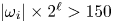 $|\omega _i|\times 2^{\ell } > 150$ are identical to those in table 3. We use
 $\varphi$ as the threshold value for the density variations
 $|\Delta \rho |$ and level-varying vorticity magnitude
 $|\omega _i|\times 2^{\ell }$. Physical parameter values are identical to those in table 3. We also provide the average percentage,
 $\bar {p}_\ell$, of the region
 $x\in [-1.5R_0,1.5R_0]$,
 $y\in [-1.5R_0,1.5R_0]$ and
 $z\in [0,5R_0]$ that is resolved by a particular grid level
 $\ell$.

We first consider the statistics of  $p_\ell$ through averages and probability density functions (p.d.f.s). The averages in table 5 show that as we increase the finest AMR level
 $\ell _{max}$, more of the region of interest is resolved at subsequently finer levels. In figure 14, the p.d.f.s for the coarsest simulations,
 $\ell _{max}=1$, are quite noisy as a result of the discrete nature of the tagging criteria, since grids generally containing
 $8^{3}$ or
 $16^{3}$ cells are tagged based on the refinement criteria, as opposed to tagging individual cells. As
 $\ell _{max}$ increases, the p.d.f.s become smoother as a result of the higher resolution, allowing the refinement criteria to resolve more localized regions of the flow. Overall, these statistics imply that if convergence is achieved, then it is very unlikely to be the result of under-resolved complex flow features. In particular, with each increase of
 $\ell _{max}$, the ‘effective’ resolution doubles and essentially the same fraction of the region is replaced by one finer level
 $\ell$.
P.d.f.s of  $p_\ell$ for the region
 $x\in [-1.5R_0,1.5R_0]$,
 $y\in [-1.5R_0,1.5R_0]$ and
 $z\in [0,5R_0]$ that is resolved by a particular grid level
 $\ell$. In each case,
 ${Ri}_0=20.0$. Plots are for: (a)
 $Re_0= 100$,
 $l_{max}=1$; (b)
 $Re_0= 316$,
 $l_{max}=1$; (c)
 $Re_0= 1000$,
 $l_{max}=1$; (d)
 $Re_0= 100$,
 $l_{max}=2$; (e)
 $Re_0= 316$,
 $l_{max}=2$; (f)
 $Re_0= 1000$,
 $l_{max}=2$; (g)
 $Re_0= 100$,
 $l_{max}=3$; (h)
 $Re_0= 316$,
 $l_{max}=3$; (i)
 $Re_0= 1000$,
 $l_{max}=3$; (j)
 $Re_0= 100$,
 $l_{max}=4$; (k)
 $Re_0= 316$,
 $l_{max}=4$; (l)
 $Re_0= 1000$,
 $l_{max}=4$.

We assess convergence using four metrics: streamwise fluxes, self-similar variables, turbulent kinetic energy (averages and spectra), and p.d.f.s of each vorticity component. The specific streamwise fluxes that we use are the time averages of mass flux and density-weighted kinetic energy flux, defined respectively as
 \begin{equation} \overline{\mathcal{M}}(z) \equiv \displaystyle{\dfrac{1}{T}\int_{t_0}^{t_f} \int_A \rho u_z \,{\rm d}{A} \,{\rm d}d{t}}, \quad \overline{\mathcal{D}}(z) \equiv \displaystyle{\dfrac{1}{T}\int_{t_0}^{t_f} \int_A \frac{1}{2}\rho(\boldsymbol{u}\ \boldsymbol{\cdot}\ \boldsymbol{u}) u_z \,{\rm d}d{A} \,{\rm d}d{t}}, \end{equation}
where  $\overline {(\,\cdot\,)}$ denotes a time average. The similarity variables that we consider are the centreline density discrepancy
 $1-\bar {\rho }_c/\rho _\infty$, and streamwise velocity
 $\bar {u}_c/U_0$, where
 $\bar {\rho }_c=\bar {\rho }(r=0,z)$ and
 $\bar {u}_c=\bar {u}_z(r=0,z)$, as well as the flow widths where
 $\bar {Y}_{He}$ and
 $\bar {u}_z$ have decayed to 50 % of their centreline values (denoted
 $\delta _Y$ and
 $\delta _u$, respectively). For the turbulent kinetic energy, we show fields of
 $\langle u_i' u_i' \rangle /2$, where
 $\langle \,{\cdot }\,\rangle$ denotes a temporal and azimuthal average, and
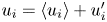 $u_i = \langle u_i \rangle + u'_i$. We also compute
 $\hat {u}_i^{*} \hat {u}_i/2$ as a function of frequency to indicate the spectral content of the turbulent kinetic energy, where
 $\hat {u}_i$ represents the Fourier transform in time of the signal
 $u_i$, and the superscript
 $*$ represents the complex conjugate. The p.d.f.s of the vorticity components are intended to highlight small-scale features of the flow. We do not consider directly convergence of the puffing frequency because of the difficulty in measuring a single frequency for the turbulent plumes, as discussed in § 3.5.
In figure 15, we show  $\overline {\mathcal {M}}$ and
 $\overline {\mathcal {D}}$ for the different resolutions at
 ${Ri}_0=20$. All of the data are well-converged for
 $\ell _{max} \geq 2$, indicating that using
 $\ell _{max}=3$, as in the present study, provides good convergence of global statistics. For
 $\ell _{max}=1$, the numerical diffusion is high, resulting in a distinct difference in the dynamics (not shown here), similar to the transition to turbulence discussed in § 3. The fact that we see convergence at relatively coarse resolutions is not surprising because the fluxes are generally associated with entrainment, which is a large-scale property of the flow and does not require very fine resolution to achieve convergence.
(a–c) Mass flux  $\overline {\mathcal {M}}$, and (d–f) density-weighted kinetic energy
 $\overline {\mathcal {D}}$, for various maximum levels of AMR of (a,d)
 ${Ri}_0=20$,
 ${Re}_0=100$, (b,e)
 ${Ri}_0=20$,
 ${Re}_0=316$, and (c,f)
 ${Ri}_0=20$,
 ${Re}_0=1000$.

Figure 16 shows self-similar quantities computed from the time-averaged density and velocity fields. These quantities include the centreline density discrepancy, the centreline velocity, the flow width based on density, and the flow width based on streamwise velocity. All of the simulations show good agreement between  $\ell _{max}=3$ and
 $\ell _{max}=4$, particularly in the puffing region of the flow (i.e.
 $z/R_0 < 1$), which provides further validation of our choice of
 $\ell _{max}=3$ used here. The few discrepancies are almost exclusively beyond the neck of the plume. Consequently, we do not expect any of the discrepancies to affect the temporal variability in the very near field below the neck of the plumes.
(a–c) Centreline density discrepancy  $1-\bar {\rho }_c/\rho _\infty$, (d–f) centreline velocity
 $\bar {u}_c/U_0$, (g–i) the flow width using helium mass fraction
 $\delta _Y$, and (j–l) the flow width using streamwise velocity
 $\delta _u$, for various maximum levels of AMR of (a,d,g,j)
 ${Ri}_0=20$,
 ${Re}_0=100$, (b,e,h,k)
 ${Ri}_0=20$,
 ${Re}_0=316$, and (c,f,i,l)
 ${Ri}_0=20$,
 ${Re}_0=1000$.

We next consider the turbulent kinetic energy  $\langle u_i' u_i'\rangle /2$ to assess convergence of the averages of second-order fluctuating moments, which have been shown previously to be important for ensuring that the puffing frequency is converged (Wimer et al. Reference Wimer, Lapointe, Christopher, Nigam, Hayden, Upadhye, Strobel, Rieker and Hamlington2020, Reference Wimer, Day, Lapointe, Meehan, Makowiecki, Glusman, Daily, Rieker and Hamlington2021). In figure 17, we show
 $r$–
 $z$ planes of
 $\langle u_i' u_i'\rangle /2$ for each of the convergence test cases. There is good agreement between
 $\ell _{max}=3$ and
 $\ell _{max}=4$, indicating further that the resolution used in § 3 is sufficient.
Spatial distribution of turbulent kinetic energy for (a–d)  ${Re}_0=100$, (e–h)
 ${Re}_0=316$, and (i–l)
 ${Re}_0=1000$, for simulations with (a,e,i)
 $\ell _{max}=1$, (b,f,j)
 $\ell _{max}=2$, (c,g,k)
 $\ell _{max}=3$, and (d,h,l)
 $\ell _{max}=4$. Each case has
 ${Ri}_0=20$.

Each of the previous quantities has indicated how the grid resolution affects average and global flow characteristics, rather than local small-scale structures. To investigate the latter, we plot the spectral kinetic energy  $\hat {u}_i^{*} \hat {u}_i/2U_0^{2}$ at the centreline for
 $z/R_0=0.5$ as a function of frequency
 $f$, in figure 18. The frequency is normalized by
 $\tau ^{*}$ according to (1.1). Due to the finite amount of data available along the centreline, the signals were smoothed using a moving average. From this figure, we make a number of important observations.
Temporal spectra of the turbulent kinetic energy as a function of frequency  $f$, normalized by
 $\tau ^{*}$ computed from (1.1). The spectra are computed at
 $z/R_0=0.5$ along the centreline. The dashed line corresponds to slope
 $-5/2$. Plots are for (a)
 $Re_0=100$, (b)
 $Re_0=316$, and (c)
 $Re_0=1000$.

We observe that each of the spectra peaks near  $f\tau ^{*} \approx 1$, as expected considering that the integral scale, or energy injection scale, is closely related to the time scale of the puffing frequency. As
 $f\tau ^{*}$ increases, the spectrum decreases rapidly, especially for the transitional flow. For the better-resolved turbulent cases (i.e.
 $\ell _{max} \geq 3$ and
 ${Re}_0\geq 316$), the decrease has slope approximately
 $-5/2$, which is the scaling that we would expect for inertial range dynamics in frequency space (instead of the classic
 $-5/3$ slope when using the spatial wavenumber
 $k$). For the transitional flow of
 ${Re}_0=100$, rather than an exponential decrease in the spectrum at high frequency, we see a flattening of the spectrum, possibly connected to the inverse cascade that has been noted previously in buoyancy-driven flows (Zhou Reference Zhou2017; Wimer et al. Reference Wimer, Day, Lapointe, Meehan, Makowiecki, Glusman, Daily, Rieker and Hamlington2021). Given these results, the resolution used in this study is sufficient to capture short temporal scales in the laminar and transitional cases, as well as producing the expected scaling relations in the turbulent cases.
The last metrics that we use to assess convergence are p.d.f.s of the vorticity components at  $r/R_0=0.75$ and
 $z/R_0=0.5$, each of which are shown in figure 19. This spatial location was selected because of the large amounts of vorticity present in this region. Note that
 $\langle \omega _r \rangle = \langle \omega _z \rangle = 0$ for a statistically axisymmetric flow, but
 $\omega _r' \neq \omega _z' \neq 0$ at any given instant in time. For
 ${Re}_0=100$ and
 $316$, the p.d.f.s confirm that
 $\ell _{max} \geq 3$ provides sufficient resolution since the p.d.f.s are almost identical for
 $\ell _{max} \geq 3$.
Logarithm of the p.d.f.s of vorticity components taken at  $r/R_0=0.75$,
 $z/R_0=0.5$. Line colours correspond to those in figure 18. Plots are for (a)
 $Re_0=100$, (b)
 $Re_0=316$, (c)
 $Re_0=1000$, (d)
 $Re_0=100$, (e)
 $Re_0=316$, (f)
 $Re_0=1000$, (g)
 $Re_0=100$, (h)
 $Re_0=316$, (i)
 $Re_0=1000$.

For the largest value of  ${Re}_0$ considered here (namely,
 ${Re}_0=1000$), the present simulations with
 $\ell _{max}=3$ are fully resolved for small and intermediate vorticity magnitudes. However, there is slight non-convergence for the most extreme vorticity values, where there are some remaining differences between the p.d.f.s for
 $\ell _{max}=3$ and 4. This indicates that higher-order moments of the velocity and velocity gradient are not converged for the
 ${Re}_0=1000$ case, but the convergence of global and second-order statistics provides confidence that the simulations are adequate for examining the temporal characteristics and puffing behaviour that are the focus of this study.
Finally, using the same code as in the present study (i.e. PeleLM), prior work by Wimer et al. (Reference Wimer, Day, Lapointe, Meehan, Makowiecki, Glusman, Daily, Rieker and Hamlington2021) has shown for an  ${Re}_0=1490$ helium plume that a resolution of at least 2 mm is required to capture the instability that gives rise to the Rayleigh–Taylor spikes that drive high-density fluid into the core of the plume. This was also found to be the resolution required to obtain converged puffing frequencies, and the finest scale in the present simulations (i.e. 1.95 mm) was chosen, in part, based on these prior results.
A.2. Sufficient threshold criteria
As a final test, we must also demonstrate that the AMR threshold criteria used herein are sufficient to resolve flow features of interest. This is particularly important for the most laminar case, since figure 3 shows that despite resolving the shear layer at the base of the plume at the finest level, the finest level is not present farther downstream. This indicates, based on our criteria, that the finest level is not required in order to resolve the scales of motion in the flow. The more turbulent cases are of lesser concern, since the finest level occupies much of the flow, and in § A.1 we showed that this resolution was sufficient.
To test the threshold criteria, we vary them for  ${Ri}_0=2$,
 ${Re}_0=100$, such that the majority of the flow is resolved at the finest level. Instantaneous snapshots of the density field are provided in figure 20, with grids corresponding to different AMR levels overlaid. Overall, these snapshots show essentially no qualitative difference. More quantitatively, we show centreline plots in figure 21 of mean vertical velocity and normalized turbulent kinetic energy. These statistics are in agreement for different refinement criteria.
Instantaneous snapshots of the density field for the most laminar simulation ( ${Ri}_0=2$,
 ${Re}_0=100$) for two different AMR refinement criteria. The grids are overlaid on the density field with regions surrounded by black lines corresponding to
 $\ell =3$, and regions surrounded by grey lines corresponding to
 $\ell =2$. (a) Simulation using the same criteria as in § 3. (b) Overly-resolved simulation using criteria given in table 5.

Centreline plots of (a)  $\bar {u}_z/U_0$ and (b)
 $\overline {u_i' u_i'}/2U_0^{2}$ for the
 ${Ri}_0=2$,
 ${Re}_0=100$ laminar plume with two different AMR criteria.


 Open access

