


Introduction
Habitat loss is the primary driver of biodiversity impoverishment (van Vuuren et al. Reference van Vuuren, Pereira, Lodge, Alder, Dobson and Wolters2005, Díaz et al. Reference Díaz, Settele, Brondízio, Ngo, Agard and Arneth2019). To alleviate the negative impacts of habitat loss on biodiversity, many countries have established legal mechanisms to compensate for deforestation whenever it is inevitable or has already occurred and cannot be reversed (Bull et al. Reference Bull, Suttle, Gordon, Singh and Milner-Gulland2013). Although such biodiversity offset policies have the potential to mitigate biodiversity loss from deforestation (ten Kate et al. Reference ten Kate, Bishop, Bayon, ten Tate, Bishop and Bayon2004), there is still an ongoing debate as to when offsets are feasible and how they should be performed to effectively conserve biodiversity (Moilanen & Kotiaho Reference Moilanen and Kotiaho2018, zu Ermgassen et al. Reference zu Ermgassen, Baker, Griffiths, Strange, Struebig and Bull2019, de Mello et al. Reference de Mello, Fendrich, Sparovek, Simmonds, Maron and Tavares2021b). In this context, understanding which biota are being targeted in a biodiversity offset policy and identifying ecologically equivalent areas for compensation are often challenging (Maron et al. Reference Maron, Ives, Kujala, Bull, Maseyk and Bekessy2016, Moilanen & Kotiaho Reference Moilanen and Kotiaho2018, Moilanen et al. Reference Moilanen, Kujala and Mikkonen2020, de Mello et al. Reference de Mello, Fendrich, Sparovek, Simmonds, Maron and Tavares2021b).
Brazil is a megadiverse country that established a biodiversity offset policy for private lands in 1998. According to these rules, a landowner whose property did not conserve the minimum percentage of native vegetation established by law (‘legal reserve’ (LR); Appendix S1) could compensate for deforestation in an ecologically equivalent area elsewhere rather than restore their property (de Freitas et al. Reference de Freitas, Sparovek, Mörtberg, Silveira, Klug and Berndes2017, de Mello et al. Reference de Mello, Fendrich, Sparovek, Simmonds, Maron and Tavares2021b). Brazilian regulation on legal reserve compensation (LRC) can be described as an averted loss mechanism (Maron et al. Reference Maron, Hobbs, Moilanen, Matthews, Christie and Gardner2012) that involves two properties: (1) the donor property, which does not have enough native vegetation cover to assign its LR (‘impact site’ as defined by Maron et al. Reference Maron, Hobbs, Moilanen, Matthews, Christie and Gardner2012); and (2) the receptor property, which houses the donor property’s LR (‘offset site’ as defined by Maron et al. Reference Maron, Hobbs, Moilanen, Matthews, Christie and Gardner2012). The regulation defined some criteria to ensure ecological equivalence between the deforested land and the offset site (Table S1). These rules remained in effect until 2012, when the Brazilian government, under intense pressure from the agribusiness sector (Nepstad et al. Reference Nepstad, McGrath, Stickler, Alencar, Azevedo and Swette2014), created the New Forest Code (NFC).
The NFC brought about three changes that notably weakened LR biodiversity’s main offset rules (Table S1). According to the former rules, donor and receptor sites should be in the same watershed and should have the same ecosystem and same ecological importance. The elimination of two ecological criteria (same ecological importance and same ecosystem) allowed the use of ecologically distinct areas for biodiversity offset, which could lead to the extinction of endangered ecosystems in the impact site while conserving less threatened ecosystems in the receptor property. The increase in the allowed spatial scale with the elimination of the watershed criteria may concentrate LRs in regions subjected to low deforestation pressure instead of protecting those subjected to higher deforestation rates (Gordon et al. Reference Gordon, Bull, Wilcox and Maron2015). These changes have allowed landowners to adopt cheaper and less effective solutions when assigning their LRs (Sparovek et al. Reference Sparovek, Berndes, Barretto and Klug2012), such as assigning offset sites in already protected areas (de Freitas et al. Reference de Freitas, Sparovek, Mörtberg, Silveira, Klug and Berndes2017).
The Brazilian Cerrado is the most diverse tropical savannah on Earth (Eiten Reference Eiten1994), and, due to the high degree of habitat loss, it is considered a global priority for biodiversity conservation (Myers et al. Reference Myers, Mittermeier, Mittermeier, Da Fonseca and Kent2000). Deforestation in the biome has significantly increased in recent years, from 6300 km2 in 2019 to 11 000 km2 in 2023, even surpassing the rate of deforestation in the Amazon (INPE 2024). For many taxonomic groups, such as anurans, small mammals and plants, the Cerrado species composition is highly heterogeneous in space, and therefore beta diversity, defined as similarity in community composition (Whittaker Reference Whittaker1960), is high (Bridgewater et al. Reference Bridgewater, Ratter and Ribeiro2004, Valdujo et al. Reference Valdujo, Carnaval and Graham2013, Carmignotto et al. Reference Carmignotto, Pardini and de Vivo2022). Contrastingly, if two communities have the same species composition, beta diversity equals zero.
Therefore, to ensure ecological equivalence between the receptor and donor properties in a biodiversity offset, beta diversity between them must be low (de Mello et al. Reference de Mello, Fendrich, Borges-Matos, Brites, Tavares and da Rocha2021a). Beta diversity generally increases with spatial distance between sites (Morlon et al. Reference Morlon, Chuyong, Condit, Hubbell, Kenfack and Thomas2008), and an increase in the spatial scale chosen for biodiversity offset may result in low ecological equivalence (i.e., high beta diversity) between receptor and donor sites. Therefore, the current LR biodiversity offset rules are expected to cause biodiversity losses in highly diverse and threatened Cerrado communities.
In this study, we tested whether the current rule for LRC can ensure tree conservation in the Cerrado biome. We also simulated LRC under the old rules (using watersheds as spatial scales admitted for biodiversity offset) to investigate whether it effectively conserves tree diversity. Finally, we simulated different spatial scales using the old rule spatial scale (watersheds) and a similarity index to propose a new approach to LRC in the Cerrado.
We used tree species as a model group, three different watershed limits as spatial units and three similarity levels to simulate possible trades of LR areas between donor and receptor properties. First, we modelled the potential geographical distribution of Cerrado tree species to determine the floristic composition of watersheds at three watershed levels that represent distinct spatial scales. We then simulated many potential LRCs to calculate the expected species loss at different spatial scales and similarity levels between properties. Here, we discuss the expected impacts of the current rules for LR biodiversity offsets on biodiversity conservation in the Cerrado.
Materials and methods
Defining spatial scales
The Cerrado biome was delimited using an official map of Brazilian biomes (IBGE 2019).
We defined three scenarios for our simulations. The ‘Current Rule’ is a scenario that uses actual rural property delimitation to simulate possible LRC under the current law. For this scenario, we used property delimitation data from the Cadastro Ambiental Rural (CAR; Rural Environmental Registry), a mandatory electronic record for Brazilian rural properties (CAR 2024). Properties were randomly selected from the CAR database using the sample function in R (R Core Team 2015). The ‘Old Rule’ scenario used watershed delimitations to simulate possible LRC under former Forest Code rules. The ‘Proposed Rule’ scenario combined watershed delimitation and a similarity index to simulate a novel proposed LRC.
Watersheds were defined according to a map that divides the Brazilian territory into six levels of basins (watersheds), adopting the codification proposed by Otto Pfafstetter to define the limits of the watersheds (ANA 2012). We adopted Ottos 3, 4 and 5 for the analysis. At the highest resolution level (i.e., Otto7), basins are delimited by the smallest area of contribution of the source, and as the number decreases, the spatial scale increases (i.e., Otto6, Otto5, etc.).
Species occurrence data
Cerrado tree occurrence data were compiled from Mews et al. (Reference Mews, Pinto, Eisenlohr and Lenza2014) and Françoso (Reference Françoso2014). To represent most of the LR vegetation across the entire biome, we selected only tree species that occur in savannah vegetation (i.e., Cerrado sensu stricto), thus excluding species that are restricted to gallery forests and dense savannah woodlands (see Ribeiro & Walter Reference Ribeiro, Walter and EI2008). We also excluded species with fewer than 10 occurrences to improve the performance of the climatic niche model (Pearson et al. Reference Pearson, Raxworthy, Nakamura and Townsend Peterson2007). The choice of a low minimum occurrence threshold is important because less frequent species drive most differences in composition between phytogeographically distinct regions within the Cerrado (Bridgewater et al. Reference Bridgewater, Ratter and Ribeiro2004). We checked the consistency between the geographical localization of each occurrence and other information available in the database. We also checked whether points located distantly from others (outliers) were compatible with the geographical distribution of each species reported in the literature (Flora do Brasil 2020, 2021). Points with any inconsistencies were excluded. The filtered database had 17 720 occurrences of 126 tree species.
Environmental variables
We obtained 35 environmental variables from the CliMond Project (Kriticos et al. Reference Kriticos, Webber, Leriche, Ota, Macadam and Bathols2012) and five from the Consortium for Spatial Information (Zomer et al. Reference Zomer, Bossio, Trabucco, Yuanjie, Gupta and Singh2007, Reference Zomer, Trabucco, Bossio and Verchot2008, Jarvis et al. Reference Jarvis, Reuter, Nelson and Guevara2008). These 40 variables were subjected to a correlation test to check for collinearity, and those showing a correlation greater than 80% with other variables were excluded (Kramer-Schadt et al. Reference Kramer-Schadt, Niedballa, Pilgrim, Schröder, Lindenborn and Reinfelder2013), resulting in 16 environmental variables for running the analysis (Table S2). These variables were rescaled to a spatial resolution of 20 × 20 km, which set the minimum pixel size in the model (Legendre Reference Legendre1993, Boria et al. Reference Boria, Olson, Goodman and Anderson2014). The chosen scale minimizes georeferencing errors in species occurrence databases (Santana et al. Reference Santana, de Siqueira, Saraiva and Correa2008). It also minimizes the effects of biological interactions (i.e., competition) on the distribution of species, as two species may be found in the same pixel (i.e., in the same landscape) but not at the same site (Araújo & Guisan Reference Araújo and Guisan2006). Points from any given species in the same pixel were considered as single points to avoid spatial autocorrelation in the data (Legendre Reference Legendre1993, Boria et al. Reference Boria, Olson, Goodman and Anderson2014).
Climatic niche modelling
To predict the climatic niche of species, we used the Maxent algorithm (Phillips et al. Reference Phillips, Anderson and Schapire2006), which produces more precise models even with low numbers of occurrence points (Pearson et al. Reference Pearson, Raxworthy, Nakamura and Townsend Peterson2007, Wisz et al. Reference Wisz, Hijmans, Li, Peterson, Graham and Guisan2008). Maxent algorithms can produce distribution maps with comparable accuracy to ensemble methods (Kaky et al. Reference Kaky, Nolan, Alatawi and Gilbert2020). The occurrence points of each species were partitioned into three replicates of the same size (i.e., the same number of points) to increase accuracy (cross-validation). We converted the species occurrence probability map into a presence/absence map using Maximum Training Sensitivity Plus Specificity, which is adequate for our conservation objectives because it focuses on minimizing errors of omission as much as possible while avoiding commission errors (Liu et al. Reference Liu, Berry, Dawson and Pearson2005, Cao et al. Reference Cao, DeWalt, Robinson, Tweddale, Hinz and Pessino2013), and it performs well when only presence data are available (Liu et al. Reference Liu, White and Newell2013). We evaluated the performance of the models using the binomial test and true skill statistic (TSS; Allouche et al. Reference Allouche, Tsoar and Kadmon2006). Only replicates with non-random results in the binomial test (p < 0.01) and TSS values higher than 0.5 were included in the final model for each species. The final model was obtained by multiplying the replicate models for each species if at least two replicates met the criteria. Any species with a single replicate meeting the criteria were excluded from the analyses.
To determine the tree species composition of watersheds (under ‘Old Rules’ and ‘Proposed Rules’ scenarios) or rural properties (under the ‘Current Rule’ scenario), we first calculated the percentage area of each spatial unit (watersheds or rural properties depending on the scenario) that the spatial model of each species occupied. A species was considered present in a spatial unit only if its model covered at least 50% of its spatial unit area. Hence, the tree species composition in each unit area comprised all species, with the final model covering at least 50% of the unit area. We used this 50% threshold to avoid considering that a species whose model occupied only a small portion of the spatial unit could be counted as present in the entire spatial unit. As we aimed to simulate possible LR compensations, we had to ensure that the species were present at the impact and donor sites.
This analysis was performed in the R statistical environment (R Core Team 2015) using the packages rgeos (Bivand et al. Reference Bivand, Rundel, Pebesma and Hufthammer2016), maptools (Lewin-Koh et al. Reference Lewin-Koh, Bivand, Pebesma, Archer, Baddeley and Bibiko2011), rgdal (Bivand et al. Reference Bivand, Tim and Rowlingson2021) and raster (Hijmans & van Etten Reference Hijmans and van Etten2014).
Spatial analysis of beta diversity
To assess the extent to which different spatial units shared a tree species composition that was sufficiently similar to allow for LRC, we calculated beta diversity between spatial units using the Jaccard index. We then performed a cluster analysis of the spatial units as a function of their similarity in species composition using the unweighted arithmetic average clustering method (UPGMA; Legendre & Legendre Reference Legendre and Legendre2012). The analysis was repeated in the ‘Proposed Rule’ scenario for nine distinct scenarios that encompassed all possible combinations of three watershed levels (Ottos 3, 4 and 5 according to the Brazilian National Agency of Waters) and three minimum similarity thresholds (70%, 80% and 90%) for forming groups. We denominated similar groups as interchangeable watershed groups (IWGs). Therefore, if a pair of donor and receptor properties belong to the same IWG, similarity between them is equal to or above the specified threshold. Contrastingly, if the properties are in different IWGs, similarity between them is below the threshold.
Considering different watershed levels in the analysis allowed us to assess the scale dependency of species similarity among the watersheds. The combination of different watersheds levels and similarity thresholds determines the degree of restriction for implementation of LRC. For instance, a threshold of 90% similarity indicates that LRC can only occur between properties located within watersheds with almost identical tree species compositions (i.e., c. 90% of common species from the total number of species in a given pair of watersheds). On the other hand, a similarity threshold of 70% is less restrictive, as it allows for LRC between properties located within watersheds that are not as similar in species composition. This analysis was performed in the R statistical environment (R Core Team 2015) using the vegan package (Oksanen et al. Reference Oksanen, Legendre, O’Hara, Stevens, Oksanen and Suggests2007).
Calculating species loss under distinct scenarios
We analysed different scenarios simulating old LRC rules (‘Old Rule’ scenario, adopting Otto3, Otto4 and Otto5 watersheds levels), current LRC rules (‘Current Rule’ scenario) and the ‘Proposed Rule’ incorporating vegetation similarity indices (Otto3, 70%, 80% and 90%; Otto4, 70%, 80% and 90%; Otto5, 70%, 80% and 90%).
To measure the potential loss of tree species (SL) in the distinct LRC scenarios, we calculated a distance matrix between all pairs of adopted spatial units (watersheds in ‘Old Rule’ and ’Proposed Rule’ scenarios or rural properties in the case of the ‘Current Rule’ scenario) using number of shared species (J) as the input. We then calculated each spatial unit species richness (R) and subtracted the shared species (J) for each species as in Equation 1:
 $$\rm SL = R - J $$
According to the new legislation, LRC can be realized anywhere within the Cerrado biome; however, if the properties are located in different states, LRC must be accomplished within a priority area for conservation. Therefore, for the ‘Current Rule’ and ‘Proposed Rule’ scenarios we used a map of priority areas for conservation developed by the Brazilian Ministry of the Environment (available at http://i3geo.mma.gov.br) to determine all possibilities of LRC between different states.
In the ‘Old Rule’ scenario, we determined all possible LR compensations without constraining LRC to priority areas for conservation; in this case, LRC could be realized anywhere within the Cerrado biome. We ran the analysis at three watershed levels, with each watershed treated as a single floristic community.
All analyses were performed in the R statistical environment (R Core Team 2015) using the vegan package (Oksanen et al. Reference Oksanen, Legendre, O’Hara, Stevens, Oksanen and Suggests2007).
Results
A total of 343 models out of 372 (92%) met the two established criteria (binomial test and TSS). Five species had fewer than two replicate models that met the criteria and were excluded from the analysis. Among the remaining 119 species, 58 were widely distributed within the Cerrado biome, according to Bridgewater et al. (Reference Bridgewater, Ratter and Ribeiro2004). The environmental variables that contributed most to the models were the seasonal humidity index (in 37% of all models) and precipitation of the wettest week (26%), which were the most important in 63% of all models. The third most important environmental variable was elevation, which was observed in 13% of all the models.
Old Rule
Analyses under the ‘Old Rule’ scenario were performed at three different watershed spatial scales (Otto3, Otto4 and Otto5; see ‘Materials and methods’ section). There were 114, 760 and 4029 watersheds at Otto3, Otto4 and Otto5, respectively.
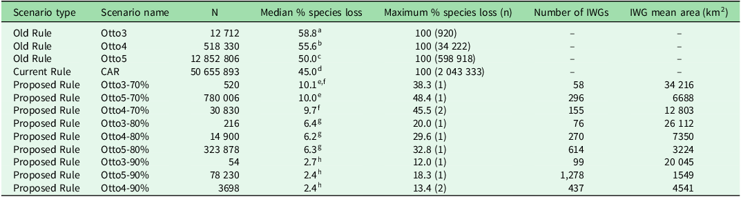
At Otto3, we simulated 12 712 LRCs, observing 58.8% median species losses between the donor and impact sites (Table 1). A total of 920 simulated compensations resulted in 100% species loss. The LRC under Otto4 was simulated 518 330 times, with a median species loss of 55.6% (Table 1). Complete species loss was observed in 34 222 simulated LRCs. In Otto5, 12 852 806 LRCs were simulated. We verified a median species loss of 50% and a total of 598 918 LRC simulations with no common species between the donor and impact sites (Table 1).
Median and maximum percentage species losses in distinct legal reserve compensation (LRC) scenarios. N indicates the number of simulated compensations used to calculate species losses in each scenario; n in the fifth column represents the number of simulations in which the maximum species loss occurred. Each interchangeable watershed group (IWG) is a group of watersheds sufficiently similar in tree species composition to allow for the LRC between any pair of watersheds in the group. Different superscript letters indicate significant differences between median percentages (Mann–Whitney test, p < 0.05, with Holm correction).

CAR = Cadastro Ambiental Rural.
Current Rule
The LRC ‘Current Rule’ was simulated using 10 000 real property limits. A total of 50 655 893 LRC simulations were performed for this scenario. The median species loss under this scenario was 45%. A total of 2 043 333 LRC simulations presented a 100% species loss, with no common species between the donor and impact sites (Table 1).
Proposed Rule
The cluster analysis of watersheds as a function of their similarity in terms of tree species composition produced groups within which watersheds were sufficiently similar to allow for LRC between pairs of watersheds (i.e., 70%, 80% or 90% similarity within groups depending on the scenario; Table 1). The number of IWGs varies widely among the nine ‘Proposed Rule’ scenarios. As expected, the lower the similarity for forming watershed groups, the more IWGs are generated across all watershed levels (Table 1).
While the scenario Otto5-90% presented 1278 IWGs with a mean area of 1549 km2, the scenario Otto3-70% presented only 58 IWGs with a mean area of 34 216 km2. Even within each watershed level, the area of distinct IWGs varied substantially (Fig. 1).
Scenarios proposed for legal reserve compensation in the Brazilian Cerrado, incorporating vegetation similarity indices. The nine scenarios included all combinations of the three watershed levels (Otto3, Otto4 and Otto5) and three similarity thresholds for forming groups (70%, 80% and 90%). In each scenario, different colours indicate interchangeable watershed groups; that is, groups of watersheds sufficiently similar in tree species composition to allow for legal reserve compensation between any pair of watersheds in the group.

There was no significant difference between different watershed levels within each similarity index adopted (Kruskal–Wallis analysis, Mann–Whitney test, p < 0.05 with Holm correction), except for Otto5-70%, which was significantly different from Otto4-70% (p = 0.00012083).
Some of the ‘Current Rule’ and the ‘Old Rule’ scenario LRCs resulted in 100% species loss, meaning no species that existed at the impact site occurred at the donor site. No 100% species losses occurred in any of the ‘Proposed Rule’ scenarios, showing the benefit of adopting the similarity index. The range of species losses in the ‘Proposed Rule’ scenario varied from 12% (Otto3-90%) to 48.3% (Otto5-70%). If LR exchanges are constrained within IWGs, the percentage of potentially lost species is remarkably lower, especially in scenarios with 90% similarity (c. 3% species loss).
The frequency of species losses was remarkably variable among the scenarios, with flat distributions in scenarios without similarity indices and a J-shaped distribution in scenarios with similarity indices; complete species loss was more frequent in the scenarios without a similarity index (Fig. S1).
Discussion
The current Brazilian rules for biodiversity offsets on private lands do not ensure ecological equivalency between donor and receptor properties in the Cerrado. Our simulations showed that compensating for habitat loss in a randomly assigned site within the Cerrado biome leads to highly variable outcomes, with a median of c. 45% and a maximum of 100% tree species loss. The same situation was observed in the ‘Old Rule’ scenario.
In contrast, setting a minimum similarity threshold between watersheds allows for the establishment of LRCs resulting in much smaller species losses. Even a low similarity threshold of 70% is sufficient to reduce the median species loss to 10%, and median losses may be reduced to 3% with a threshold of 90% similarity. The LRCs with no common species between impact and donor sites (maximum species losses of 100%) observed in ‘Current Rule’ and ‘Old Rule’ scenarios shows that the adoption of these rules allows compensation in areas with entirely different species, thus leading to losses in biodiversity and ecosystems services (de Mello et al. Reference de Mello, Fendrich, Borges-Matos, Brites, Tavares and da Rocha2021a).
IWGs tended to be larger in the core region than at the periphery of the Cerrado (Fig. 1), indicating that the central Cerrado presents high homogeneity in tree species composition at the watershed scale (i.e., low beta diversity between watersheds). Therefore, the answer to the question ‘what is the best spatial scale for LRC in the Cerrado?’ is: ‘it depends on which part of the Cerrado’. LRC should be more restrictive near the periphery of the Cerrado, where tree species composition varies at a smaller spatial scale than in its core region.
In Brazil, 44% of the territory is private land, reaching 73% in the Central Western region, occupied mainly by the Cerrado (Sparovek et al. Reference Sparovek, Reydon, Guedes Pinto, Faria, de Freitas and Azevedo-Ramos2019). Only 7.94% of the biome is within public protected areas (Gonçalves et al. Reference Gonçalves, Gomes and Nabout2020). Therefore, LRs play a prominent role in the legal protection of native vegetation in the Cerrado, particularly in geographical areas that are poorly represented in public protected areas (Metzger et al. Reference Metzger, Bustamante, Ferreira, Fernandes, Librán-Embid and Pillar2019), such as flat lands and tabletops (Marques et al. Reference Marques, Nogueira, Martins and Sawaya2010). This emphasizes the importance of efficient LRC policies to conserve native vegetation in private lands.
The protection of a completely distinct set of species through LRC in a floristically dissimilar area can lead to the global extinction of species with restricted geographical ranges (Develey & Pongiluppi Reference Develey and Pongiluppi2010, Freitas Reference Freitas2010, Marques et al. Reference Marques, Nogueira, Martins and Sawaya2010, Toledo et al. Reference Toledo, de Carvalho-e-Silva, Sánchez, de Almeida and Haddad2010). Therefore, similarity in species composition between watersheds must be considered in order to implement LR offsets that effectively conserve Cerrado biodiversity on private lands.
Our results indicate that the amount and seasonality of precipitation and altitude are key drivers of tree species distribution in the Cerrado. Similar variables have been found to influence the Cerrado species composition of lizards (Nogueira et al. Reference Nogueira, Colli and Martins2009), anurans (Valdujo et al. Reference Valdujo, Carnaval and Graham2013) and small mammals (Ribeiro et al. Reference Ribeiro, Ricklefs and Marinho-Filho2020), suggesting that there may be some congruence in the distribution of different taxonomic groups within the biome. If biodiversity data are unavailable to establish an effective LR offset, similarity in abiotic conditions between watersheds can be used as a proxy for similarity in species composition (de Mello et al. Reference de Mello, Fendrich, Borges-Matos, Brites, Tavares and da Rocha2021a). In this case, we suggest that compensation in the Cerrado should be implemented in areas with similar precipitation regimes and altitudes.
Although spatial pattern of biodiversity should be a key criterion for the compensation of habitat loss, the best scenario in terms of biodiversity offset policy must be tailored to the socio-environmental landscape context (Moilanen & Kotiaho Reference Moilanen and Kotiaho2018, de Mello et al. Reference de Mello, Fendrich, Sparovek, Simmonds, Maron and Tavares2021b). An adequate biodiversity offset policy must be established through the participation of multiple stakeholders (Bull et al. Reference Bull, Suttle, Gordon, Singh and Milner-Gulland2013, Mansourian & Vallauri Reference Mansourian and Vallauri2014, Maron et al. Reference Maron, Ives, Kujala, Bull, Maseyk and Bekessy2016). The ‘Watershed Committees’ (Abers & Jorge Reference Abers and Jorge2005), which include representatives from civil society and government agencies or any other form of local organization, constitute an appropriate forum to guarantee this participation at the watershed level.
Biodiversity conservation and landscape management on private lands must consider the costs to landowners (Strassburg et al. Reference Strassburg, Beyer, Crouzeilles, Iribarrem, Barros and de Siqueira2019, de Mello et al. Reference de Mello, Fendrich, Borges-Matos, Brites, Tavares and da Rocha2021a). For instance, prioritizing areas with low agricultural suitability for establishing LRs can ensure greater legislation compliance (de Mello et al. Reference de Mello, Fendrich, Sparovek, Simmonds, Maron and Tavares2021b). Maps of IWGs, as proposed here, represent a straightforward tool that should be made available to all stakeholders and decision-makers involved in LRC to reconcile biodiversity conservation and socioeconomic viability.
It is important to mention that there are no statistics available regarding how many properties have had their LRs compensated at the national level. This information is essential for evaluating the effectiveness of this important public environmental policy and should be made available on the CAR platform.
Conclusions
Our study shows that changes in rules for LRC that came with the NFC allow the establishment of LRs in areas that share no tree species with the deforested property. Therefore, the current rule is expected to strongly impact the Cerrado’s biodiversity, as LRs are vital conservation components in this biome (Metzger et al. Reference Metzger, Bustamante, Ferreira, Fernandes, Librán-Embid and Pillar2019).
Adopting criteria that consider species composition similarity between watersheds is a practical way to identify the spatial scales at which the LRC will lead to minimal species loss. The scenarios presented here can be improved by incorporating analyses of other taxonomic groups (i.e., vertebrates and invertebrates).
We hope that our study can be evaluated by legislative houses to support new regulations that can guarantee the effective conservation of biodiversity in this highly threatened biome.
Supplementary material
To view supplementary material for this article, please visit https://doi.org/10.1017/S0376892925000050.
Acknowledgements
GBdO thanks IBAMA for supporting this study. We thank two anonymous reviewers for their careful reading of our manuscript and their insightful comments and suggestions.
Financial support
This study was partially supported by the Graduate Program in Ecology at the University of Brasília. We thank IBAMA for the support in the development of this study.
Competing interests
The authors declare none.
Ethical standards
Not applicable.