

1. Introduction
The increasing need for energy saving in the land transport sector has brought many challenges for ground vehicle manufacturers to curb gas emissions, to face the depletion of fossil energy sources and to improve the range of green vehicles. An important part of the energy consumption of ground vehicles at highway speeds is related to their aerodynamic drag: it ranges from one-third for heavy trucks to four-fifths for passenger cars. The common feature between most of these ground vehicles is a blunt-based geometry inducing a massively separated flow with a low-pressure wake. These wakes have been an important subject of both academic and industrial research for years, and, as such, many studies (e.g. Littlewood & Passmore Reference Littlewood and Passmore2012; Grandemange, Gohlke & Cadot Reference Grandemange, Gohlke and Cadot2013b; Zhang et al. Reference Zhang, Liu, Zhou, To and Tu2018) have focused on simplified vehicle geometries, such as the Ahmed body (Ahmed, Ramn & Faltin Reference Ahmed, Ramn and Faltin1984) for passenger cars or more recently the simplified heavy truck model introduced by Szmigiel (Reference Szmigiel2017) and Castelain et al. (Reference Castelain, Michard, Szmigiel, Chacaton and Juvé2018), among other academic geometries. The main goal of these studies is to investigate and describe the pressure drag generation mechanisms in these wakes in order to provide general means of efficient flow control for drag reduction.
In an effort to reduce the pressure drag of three-dimensional blunt bodies, many techniques of flow control, both passive and active, have been developed (see the reviews of Choi, Jeon & Kim (Reference Choi, Jeon and Kim2008) and Choi, Lee & Park (Reference Choi, Lee and Park2014) on the topic). The distinction between these two general families of flow control relies on the introduction of additional external energy (Choi et al. Reference Choi, Jeon and Kim2008). Several passive flow control devices have long been introduced and viewed as an efficient means to reduce the drag of bluff blunt bodies. A popular passive technique is the so-called boat-tailing, which consists of large geometrical modification of the base of the body leading to a gradual reduction of the bluff body's cross-section. This passive technique has been successfully applied to reduce the pressure drag of various types of bluff blunt bodies like two-dimensional bodies (Maull & Hoole Reference Maull and Hoole1967), axisymmetric bodies (Mair Reference Mair1969) or square-section bodies (Wong & Mair Reference Wong and Mair1983; Bonnavion & Cadot Reference Bonnavion and Cadot2018, Reference Bonnavion and Cadot2019). These boat-tails are generally formed either by constant-angle surfaces with a salient edge at the upstream junction with the rest of the body, or by curved surfaces leading to a smooth junction. For constant-angle surfaces, also named flaps, Chaligné (Reference Chaligné2013), Grandemange et al. (Reference Grandemange, Mary, Gohlke and Cadot2013c), Schmidt et al. (Reference Schmidt, Woszidlo, Nayeri and Paschereit2015), Perry, Pavia & Passmore (Reference Perry, Pavia and Passmore2016), de la Cruz, Brackston & Morrison (Reference de la Cruz, Brackston and Morrison2017) and Szmigiel (Reference Szmigiel2017) showed how, with small angles up to 10–15 $^{\circ }$, the flow could stay attached to the surface, leading to drag reduction. Nevertheless, for higher angles, the flow naturally detaches from the flaps and may even lead to drag enhancement. Recently Mariotti et al. (Reference Mariotti, Buresti, Gaggini and Salvetti2017) proposed an adaptation of boat-tails by adding contoured transverse grooves on them to further delay the flow separation for aggressive boat-tailing angles, leading to improved drag reductions. Nevertheless, all these passive flow control techniques impose important geometric modifications to the basic geometry to achieve a quantifiable effect on the aerodynamic drag, with boat-tailings or flaps of typical length between
 $0.1H$ and
 $0.5H$, where
 $H$ is the characteristic dimension of the model's cross-section. These important modifications are not always suited to the geometrical constraints imposed in the road vehicle industry and they imply a definitive change of the geometry. In addition, their robustness and adaptivity are not always insured for changing flow conditions, which are of great practical interest.
Nevertheless, active control techniques have been proven to tackle efficiently the pressure drag problem without posing the problem of geometrical modifications. Oxlade et al. (Reference Oxlade, Morrison, Qubain and Rigas2015), for an axisymmetric blunt body, and Barros et al. (Reference Barros, Borée, Noack, Spohn and Ruiz2016), for the Ahmed body, have shown how the use of high-frequency (decoupled from the natural instabilities of the wake) pulsed jets just below the rear separation edge all around the base could lead to a base pressure recovery and drag reductions. By a combination of a fluidic boat-tailing effect (Smith & Glezer Reference Smith and Glezer2002) and a broadband stabilization of the wake (Dandois, Garnier & Sagaut Reference Dandois, Garnier and Sagaut2007; Vukasinovic, Rusak & Glezer Reference Vukasinovic, Rusak and Glezer2010), they showed important drag reductions for both geometries. However, these drag reductions were limited to small free-stream velocities and were shown by Barros et al. (Reference Barros, Borée, Noack, Spohn and Ruiz2016) to dramatically decrease when the free-stream velocity is increased regardless of the forcing amplitude. The partial coupling of active and passive control techniques can also be used to achieve further drag reductions for bluff blunt bodies through the use of the Coanda effect (Wille & Fernholz Reference Wille and Fernholz1965). By putting curved surfaces or inclined straight flaps tangent to small steady blowing jets, Freund & Mungal (Reference Freund and Mungal1994), Englar (Reference Englar2001) and Pfeiffer & King (Reference Pfeiffer and King2018) showed how the flow could be reattached on those surfaces in order to lead to a boat-tailing effect even more important than in the passive control case. These adjacent surfaces were further coupled to small unsteady pulsed jets by Chaligné (Reference Chaligné2013), Barros et al. (Reference Barros, Borée, Noack, Spohn and Ruiz2016), Li et al. (Reference Li, Noack, Cordier, Borée and Harambat2017) and Szmigiel (Reference Szmigiel2017) in order to increase the drag reductions observed with the use of high-frequency pulsed jets alone by Oxlade et al. (Reference Oxlade, Morrison, Qubain and Rigas2015) and Barros et al. (Reference Barros, Borée, Noack, Spohn and Ruiz2016). However, the particular mechanisms involved in the pressure drag reduction and any proper scaling laws of the phenomenon involving the main parameters, like free-stream velocity, pulsed jet frequency and amplitude or the size of the adjacent surfaces, were not made extensively explicit in these studies.
The main difference between passive boat-tails or flaps and their combination with steady or pulsed jets is the ability for the jets to reattach the flow on the surface where it would be naturally detached. The jet dynamics is of primary importance in the interaction between the separated flow and the flap geometry. Greenblatt & Wygnanski (Reference Greenblatt and Wygnanski2000) and Darabi & Wygnanski (Reference Darabi and Wygnanski2004a,Reference Darabi and Wygnanskib) studied this reattachment and separation of the flow over a canonical flap geometry of length one order of magnitude higher than the flaps used in the work of Szmigiel (Reference Szmigiel2017) for instance. They showed how the optimal jet frequency for reattaching the flow over the flap directly scaled with the free-stream velocity and the length of the flap. These aspects are of primary practical importance in large-scale applications such as the control of flow separation over an airfoil to prevent stall, as shown by Glezer, Amitay & Honohan (Reference Glezer, Amitay and Honohan2005) for instance. The work of Rinehart (Reference Rinehart2011) and Lambert, Vukasinovic & Glezer (Reference Lambert, Vukasinovic and Glezer2019) partially studied this interaction with smaller flaps and higher jet frequency but without looking for proper scaling laws of the phenomena involved and with a focus on the control of cross-flow forces rather than drag. To the best of the authors’ knowledge, no work in the literature has extensively focused on the interaction of highly unsteady pulsed jets with small surfaces of high degree of curvature and its impact on the pressure drag generation problem for bluff blunt bodies. Recently, several studies, for instance Berk, Medjoun & Ganapathisubramani (Reference Berk, Medjoun and Ganapathisubramani2017) and Stella etal. (Reference Stella, Mazellier, Joseph and Kourta2018), have focused on the fine-scale dynamic interaction between pulsed or synthetic jets and recirculating wake flows such as backward-facing steps in order to draw general scaling laws involving the formation of the pulsed jets and its influence on the recirculating wake.
The present work aims to exhaustively describe what we will call in the remainder of this paper an ‘unsteady Coanda effect’, which is shown to differ considerably from the steady Coanda effect used in a broad range of applications in the fluid mechanics field. For that, we will focus on describing the peculiar effect of small-scale curved surfaces coupled to adjacent high-frequency pulsed jets. These jets are blown at frequencies of the order of  $O(U_0/r)$ (where
 $U_0$ is the free-stream velocity and
 $r$ is the size of the curved surface). Compared with blowing frequencies one order of magnitude smaller, they offer an additional advantage in reducing the pressure drag of an Ahmed-like body. The final focus of the paper is put on providing more general scaling laws of the described phenomena, which will be of primary importance for further practical applications. The experimental apparatus designed and used for this work is detailed in § 2. A global view of the drag changes observed with extensive variation of the parameters of the problem is presented in § 3. Based on these variations, a physical discussion on the time scales of the unsteadiness of the separation from the curved surface is introduced. From then on, a finer investigation into the vorticity dynamics at separation relates the observed drag changes to the way the flow is manipulated, and we provide scaling laws describing the involved mechanisms through an inviscid-flow model in § 4. A detailed picture of the peculiar flow mechanisms leading to additional drag reduction at high frequency is presented in § 5 with particular attention paid to the flow curvature near the separation. The inviscid-flow model is additionally extended to further discuss the coupling between
 $f$ and
 $r$ and to identify an optimal forcing frequency. Finally, in § 6 we extend the discussions to provide more general implications of the present work before giving our concluding remarks.
2. Experimental set-up
This section describes the set-up of the bluff body in the wind tunnel and the different measurement techniques used. In addition, we give the details of the pneumatic forcing system used for drag manipulation and describe the data analysis.
2.1. Wind-tunnel facility and model geometry
The experiments are performed inside the working section of a subsonic closed-loop wind tunnel of  $2.4~\text {m}$ width and
 $2.6~\text {m}$ height. The turbulence intensity of the upstream flow is of the order of
 $0.3\,\%$ at most operating conditions, with flow homogeneity better than
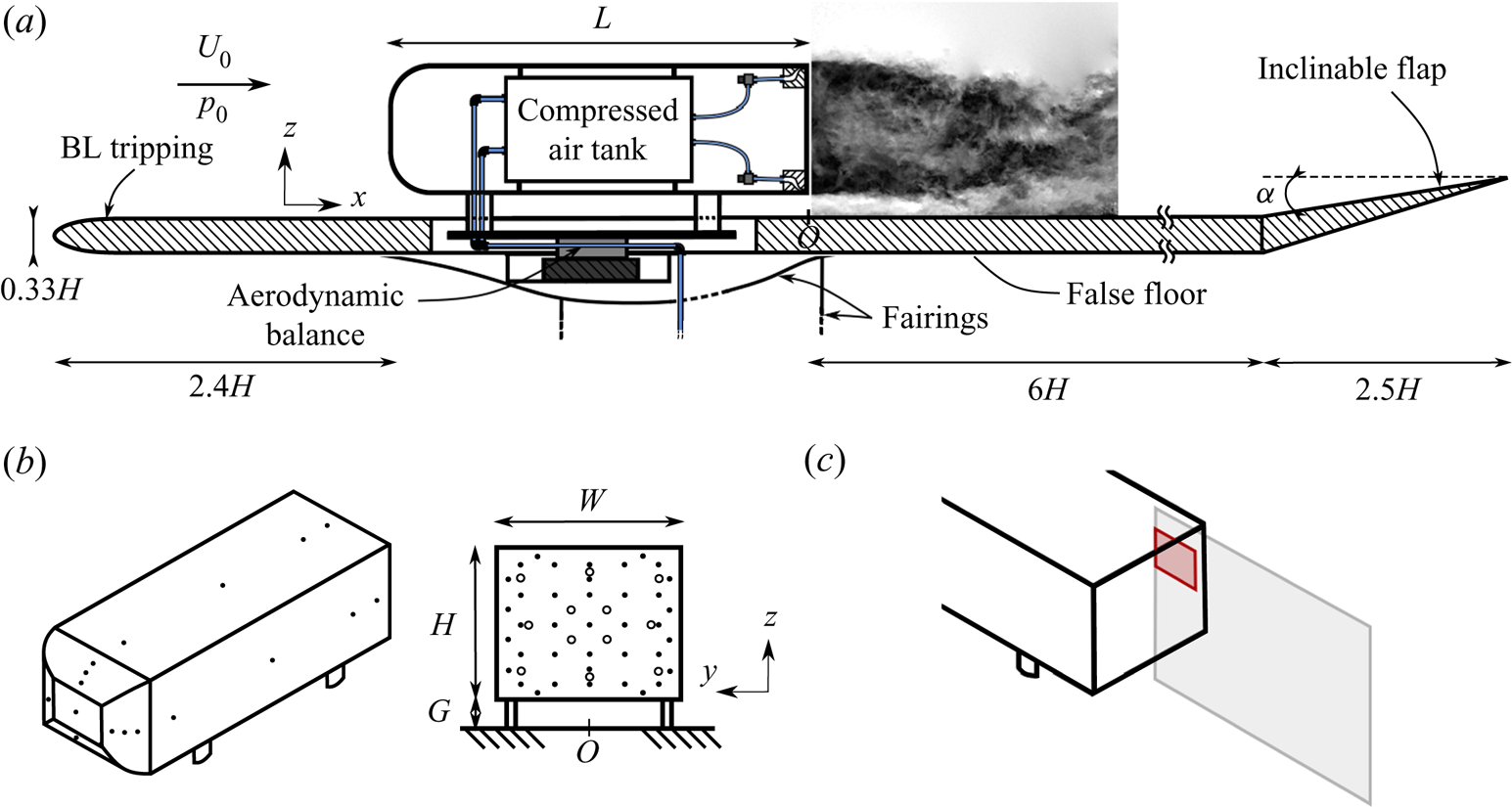
 $0.5\, \%$. A sketch of the bluff-body arrangement inside the working section is given in figure 1(a). The front of the model consists of curved edges rounded with a non-constant radius leading to a smooth curvature transition with the flat side surfaces of the model. This is aimed at minimizing the flow detachment just after the rounded front surface, limiting its impact on the downstream wake flow (Spohn & Gilliéron Reference Spohn and Gilliéron2002). The model with height
 $H = 0.3~\text {m}$, width
 $W = 0.36~\text {m}$ and length
 $L = 1~\text {m}$ (with an aspect ratio
 $H/W = 0.83$ slightly higher than the original geometry of Ahmed et al. (Reference Ahmed, Ramn and Faltin1984)) is fixed on a raised false floor with a ground clearance
 $G = 0.05~\text {m}$, which corresponds to approximately five times the thickness of the turbulent boundary layer upstream of the model. The influence of flow blockage above the raised floor was neglected due to a low blockage ratio of
 $2.2\,\%$. An inclinable flap fixed at an upward angle of
 $\alpha = 1^{\circ }$ ends the raised floor in order to compensate for the lift and the streamwise pressure gradient generated by the whole set-up.
Experimental set-up.  $(a)$ Arrangement of the model and the false floor inside the test section.
 $(b)$ Distribution of pressure taps along the model and on the rear surface: points indicate the locations of mean pressure measurements and circles the locations of time-resolved pressure measurements.
 $(c)$ Position of the particle image velocimetry measurement planes.

For the present investigations, free-stream velocities  $U_0 = \{20, 25, 30, 35, 40\}~\textrm {m}\,\textrm {s}^{-1}$ in the test section were considered, corresponding to Reynolds numbers based on the height of the model
 $Re_H = U_0H/\nu = \{4, 5, 6, 7, 8\}\times 10^{5}$, where
 $\nu$ is the kinematic viscosity of the air at operating temperature. We use conventional notation in the Cartesian coordinate system with
 $x$,
 $y$ and
 $z$, respectively, for the streamwise, spanwise and cross-stream or transverse directions (accordingly
 $\boldsymbol {u} = (u_x,u_y,u_z)$ for the velocity field) with the origin
 $O$ arbitrarily located on the floor in the vertical plane of symmetry of the model. Unless otherwise specified, all physical quantities are normalized by
 $U_0$ and
 $H$ and by the dynamic pressure
 $0.5\rho U_0^{2}$, where
 $\rho$ is the air density at operating conditions. In the remainder of the paper, the time average of a quantity
 $\chi$ is denoted by an overbar
 $\overline {\chi }$ and a Reynolds decomposition into its time-averaged part and fluctuating part
 $\chi '$ is introduced, such that
 $\chi = \overline {\chi } + \chi '$.
2.2. Pressure measurements
To perform surface pressure measurements on the model, two different systems have been used. First, a 64-channel ESP-DTC pressure scanner linked to 1 mm diameter pressure tappings around the model (35 taps on the base, see figure 1b) by  $80~\text {cm}$ long vinyl tubing was used for static pressure measurements sampled at
 $200~\text {Hz}$ with a range of
 ${\pm } 1~\text {kPa}$. In addition, 16 differential pressure sensors (SensorTechnics HCLA 02X5DB) – 12 tappings on the base, the distribution of which is given in figure 1(b), and four tappings of diameter reduced to 0.7 mm on the curved surfaces, the distribution of which is given in figure 2(a) – are used with a reduced
 $25~\text {cm}$ tubing length and proper frequency response calibration for time-resolved measurements with a bandwidth of
 $2~\text {kHz}$ (Ruiz et al. Reference Ruiz, Sicot, Brizzi, Laumonier, Borée and Gervais2009). These operate in a range of
 ${\pm }250~\text {Pa}$ (
 ${\pm }1250~\text {Pa}$ for measurements on the curved surfaces) and acquisition is performed at twice the cut-off frequency, hence
 $4~\text {kHz}$. The measurement uncertainty of both systems lies, respectively, below
 ${\pm }1.5~\textrm {Pa}$ and
 ${\pm }0.7~\textrm {Pa}$ (
 ${\pm }3.2~\textrm {Pa}$ for the measurements on the curved surfaces), which represents
 ${<}2\,\%$ of the mean base pressure.
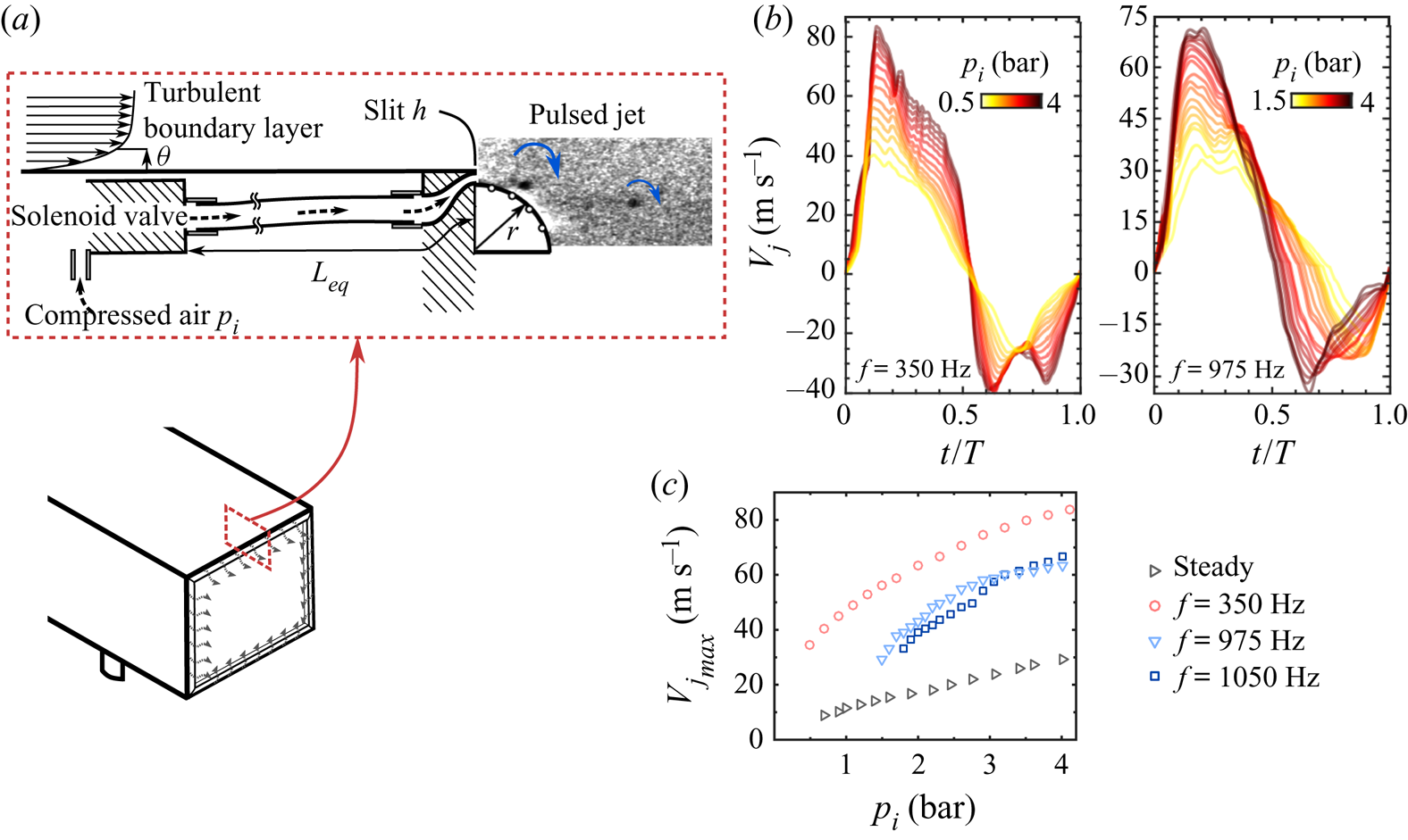
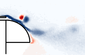
Actuation system used for forcing.  $(a)$ Arrangement of one solenoid valve, tubing system and additional curved surface generating the pulsed jets. The inset picture from the small PIV FOV visualizes small-scale vortical structures forming at the exit of the slit.
 $(b)$ Phase-averaged velocity profile at the centre of the exit plane of a slit for the forcing at
 $f = 350$ and
 $975~\textrm {Hz}$ and various inlet pressures
 $p_i$.
 $(c)$ Evolution of the maximal velocity
 $V_{j_{max}}$ with the input pressure
 $p_i$ for the different forcing frequencies used.

Pressure measurements are expressed in terms of the pressure coefficient  $C_p$ defined as
 \begin{equation} C_p = \frac{p-p_0}{0.5\rho U_0^{2}}. \end{equation}
The reference pressure  $p_0$ is taken at
 $x/H = -2$ above the model by a Pitot tube mounted at the ceiling of the test section. For each configuration studied, pressure measurements are performed over a time window of at least
 $t = 120~\textrm {s}$, which corresponds to
 $10^{4}$ convective time units
 $H/U_0$ at
 $U_0 = 25~\text {m}\,\text {s}^{-1}$. As the unforced flow behind our model presents a lateral bimodal behaviour on long time scales of the order of
 $O(10^{3} H/U_0)$ (Grandemange et al. Reference Grandemange, Gohlke and Cadot2013b), which persists when global forcing all around the base of the model is applied, this time window is not sufficient to obtain complete statistical convergence. Nevertheless, due to the important number of configurations studied involving all the parameter sweeps in this work, this time window was chosen as a compromise to keep a reasonable experiment duration and was considered as satisfactory regarding the convergence of the mean base pressure based on comparison with longer experiments and on the standard deviation of repeated measurements (
 ${<}2\,\%$ deviation from the mean value for the mean base pressure). Indeed, care was taken over the repeatability of the results by reproducing a couple of parameter sweeps. For all the configurations investigated with particle image velocimetry (PIV), the measurements were repeated 1–5 times during the PIV acquisitions for a duration of
 $t = 240~\textrm {s}$ for the cases where phase-locked measurements were taken. For the configurations involving phase-locked PIV, this leads to a total of
 $t = 1320~\textrm {s}$ (110 000 convective time units at
 $U_0 = 25~\text {m}\,\text {s}^{-1}$), which is sufficient to achieve full statistical convergence.
2.3. Aerodynamic force measurements
To quantify the effects of forcing on the drag, the model was directly mounted on a six-component aerodynamic balance (9129AA Kistler piezoelectric sensors and 5080A charge amplifier). The balance has been calibrated in-house using known masses and a system of pulleys applying pure forces, pure moments or a combination of both on the balance. A whole volume including the expected application point of the aerodynamics tensor of the model has been covered for calibration by using various level arm lengths for moments. Total measurement uncertainty is  ${<}0.6\,\%$ of the full-scale range, which represents
 ${<}1\,\%$ uncertainty in the mean drag force
 $F_x$ for instance. The pulsed jet system used for forcing induces a small thrust, which is included in the drag force measurement. In order to evaluate the contribution of the pulsed jet thrust in the measured drag, each forcing configuration is also tested at quiescent free-stream conditions. At
 $U_0 = 25~\text {m}\,\text {s}^{-1}$, for example, the thrust contribution to the total measured drag
 $F_x$ is
 ${<}3\,\%$ (at maximum when forcing is operated at the highest velocities). Drag measurements are expressed as a non-dimensional drag coefficient
 \begin{equation} C_x = \frac{F_x}{0.5\rho U_0^{2}HW}. \end{equation}
Measurements were performed simultaneously with the pressure measurements, leading to similar conclusions concerning their statistical convergence.
2.4. Velocity measurements and pressure field reconstruction
Particle image velocimetry is used to gain insight into the flow structure. Two planar two-component set-ups are used, as shown in figure 1(a): a large field of view (FOV) covering the whole recirculation region in the wake in the vertical plane of symmetry of the model (plane  $y = 0$); and a smaller FOV localized in the same plane covering the beginning of the top shear layer until
 $x/H \sim 0.35$. Both FOVs are imaged by a LaVision Imager LX
 $16~\text {Mpx}$ equipped with, respectively, a Zeiss Makro-Planar ZF 50 mm lens and a Nikon AF Micro-Nikkor 200 mm lens. A laser light sheet of 1 mm thickness is provided by a Quantel EverGreen
 $2\times 200~\textrm {mJ}$ laser, and the flow is seeded from downstream of the raised floor by atomization of mineral oil, producing
 $1~\mathrm {\mu }\textrm {m}$ diameter particles. For the small FOV, although the pulsed jets are not directly seeded, the aspiration phase of the forcing (discussed in detail in § 2.5) still allows for a weak presence of particles in the laminar flow coming from the jets when the forcing is used, which leads to satisfactory seeding of the flow. A total of 1000 image pairs are acquired at a rate of
 $4~\text {Hz}$ for each configuration studied, which is satisfactory for convergence of the second-order statistics. Image pairs are processed with Davis 8.4 with a final interrogation window of
 $16\times 16$ pixels and overlap of
 $50\,\%$, leading to a velocity vector each
 $1.2~\text {mm}$ and
 $0.15~\text {mm}$, respectively, for each field of view. Additional phase-locked measurements using as reference the command signal of the forcing system are performed for the small FOV. In this case, between 500 and 1000 images are acquired for each phase, and each pulsing period is split into 7–13 phases. For the small FOV, specific surface treatment (a thin oil coating) is applied on the curved surfaces in order to limit the influence of laser light reflections near the surface. Two additional steps are used in the processing of image pairs: a sliding minimum subtraction in order to eliminate residual laser light reflections near the curved surface; and an image translation to correct for the small displacements of the model due to relative flexibility of the aerodynamic balance, which can result in 1–2 pixels displacement on this high-magnification-factor PIV set-up.
Pressure fields were calculated from the mean PIV velocity fields using a method similar to the one used by Oxlade (Reference Oxlade2013) by explicit integration of the two-dimensional Reynolds-averaged momentum equations. Details on and validation of the method are given in appendix B.
2.5. Actuation system
In order to force the wake of the model, a series of solenoid valves are used to generate pulsed jets. A  $12~\textrm {litre}$ pressurized air tank is contained inside the model (see figure 1a). By controlling the pressure
 $p_i$ inside the tank, the magnitude of the forcing, i.e. the exit velocity of the pulsed jets, can be changed, and by controlling the actuation parameters of the solenoid valves, the frequency and duty cycle (the fraction of period during which the valve is opened) can be changed. The pressure
 $p_i$ is regulated continuously by a proportional–integral–derivative (PID) feedback controller and a flow regulator placed upstream with a precision better than
 ${\pm }0.02~\textrm {bar}$.
Pulsed jets are issued all around the base of the model through 26 slits of  $h = 1~\text {mm}$ thickness and
 $40~\text {mm}$ width. Each slit is separated from its neighbours by
 $4~\text {mm}$ and localized
 $0.5~\text {mm}$ below the base edges. The
 $h$ value is approximately
 $\theta /2$, where
 $\theta$ is the momentum thickness of the boundary layer at the trailing edge, measured by hot-wire anemometry (HWA) just after the separation edge. Each solenoid valve supplies two slits and is linked to them through semi-rigid tubing and carefully designed diffusers to allow for a smooth transition to the slit geometry. The total equivalent length of the tubing from the valve down the slit is denoted
 $L_{{eq}}$. This length fixes the frequency of the acoustic Helmholtz resonance (Kinsler et al. Reference Kinsler, Frey, Coppens and Sanders1999), which has an important impact on the exit velocity of the pulsed jets (details can be found in Haffner Reference Haffner2020). The fundamental Helmholtz resonance frequency was found to be
 $f = 350~\textrm {Hz}$. To take advantage of the resonance, we focus on driving the forcing at this particular frequency and at its odd harmonics (as the tubing system can be modelled by a closed–open acoustic duct), hence the choice of two forcing frequencies investigated in this work
 $f = 350$ and
 $1050~\textrm {Hz}$ (which is the highest accessible frequency for our forcing apparatus) in addition to the steady blowing case. To check for robustness of the results for the highest frequency forcing, we also chose a forcing frequency
 $f = 975~\textrm {Hz}$ close enough to the first odd harmonic
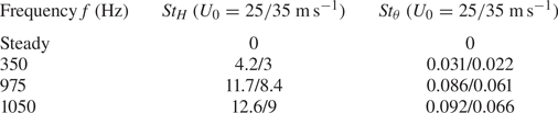
 $f = 1050~\textrm {Hz}$ but with sufficient margin compared with the limit of the forcing apparatus. These two frequencies lead to very similar results. They are specified but used indifferently in the paper for completeness of the analysis in order to take advantage of all the data acquired. These frequencies and their non-dimensional equivalents are given in table 1.
Characteristic dimensional ( $\,f$) and non-dimensional (
 $St_H$ and
 $St_{\theta }$) frequencies used for forcing:
 $St_H = fH/U_0$ is the Strouhal number based on the height of the model and
 $St_{\theta } = f\theta /U_0$ is that based on the momentum thickness
 $\theta$ of the boundary layer at the trailing edge of the model. Non-dimensional frequencies are given as indication at
 $U_0 = 25$ and
 $35~\text {m}\,\text {s}^{-1}$. For this flow, global absolute instability of the wake or vortex shedding is occurring at
 $St_H \sim 0.2$ (Grandemange et al. Reference Grandemange, Gohlke and Cadot2013b) and convective instability of the surrounding shear layers at
 $St_{\theta } \sim 0.021$ (Zaman & Hussain Reference Zaman and Hussain1981). The chosen forcing frequencies are thus mainly decoupled from the characteristic frequencies of the wake except for
 $f = 350~\textrm {Hz}$ at
 $U_0 = 35~\textrm {m}\,\textrm {s}^{-1}$.

A detailed sketch of the actuation system is given in figure 2(a) with flow visualization using the small FOV set-up where the formation of small-scale vortical structures with a characteristic size  $O(h)$ can be seen. HWA measurements were performed at the centre of the exit plane of the slits in order to characterize the forcing conditions. Additional PIV measurements (not presented here) have shown the existence of an aspiration phase at the end of the forcing cycle during which the flow is reversed. Correction of the velocity sign has thus been performed in the hot-wire time signal for the aspiration phase identified in these complementary PIV measurements. The evolution of the corrected phase-averaged exit velocity
 $V_j$ when varying
 $p_i$ on the whole operating range at
 $f = 350$ and
 $975~\textrm {Hz}$ is given in figure 2(b). The exit velocity profile is composed of a main peak followed by a trough. The peak occurs at approximately
 $t/T \sim 0.15$ and has a well-defined triangular shape. Its amplitude
 $V_{j_{max}}$ increases with increasing
 $p_i$, as shown in figure 2(c). The trough, occurring at approximately
 $t/T \sim 0.7$, is less pronounced and with more negligible variations in amplitude.
Detailed measurements at the centre of all 26 slits have allowed the homogeneity of the forcing to be quantified. The maximal velocity and the root-mean-square (r.m.s.) velocity at each slit are contained in a band of  ${\pm }5\,\%$ around the average value between all slits. The forcing amplitude is defined by
 \begin{equation} C_{\mu} = d_c\frac{S_j V_{j_{{max}}}^{2}}{S U_0^{2}}, \end{equation}
where  $S_j$ is the total section of the slits,
 $V_{j_{{max}}}$ is the peak velocity of the pulsed jets,
 $S = HW$ is the cross-section of the model, and
 $d_c$ is the effective duty cycle of the forcing based on the HWA measurements and defined as the relative period over which
 $V_j > 0$. We choose an amplitude definition based on the peak velocity in order to more fairly compare unsteady and steady forcing.
Additional curved surfaces of radius of curvature  $r = \{5,7,9,16\}h$ are placed flush to the slits in order to take advantage of a Coanda effect and to investigate their coupling with the pulsed jet forcing. The two bigger curved surfaces are instrumented with four pressure taps as sketched on figure 2(a), which were chosen to have a diameter of 0.7 mm to limit their impact on the curvature of the surfaces.
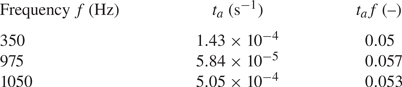
It will be shown that two characteristic time scales have to be defined in order to analyse the interaction of the pulsed jets with the curved surfaces and the consequences on the evolution of the global drag force. First, the sudden rise of the jet velocity imposes a time scale on the flow at separation. This time scale  $t_a$ is defined as
 \begin{equation} t_a = \dfrac{V_j(t')}{\left[\dfrac{\textrm{d}V_j}{\textrm{d}t}\right](t')}, \end{equation}
where  $t' = \arg \max _{t}(\textrm {d}V_j/\textrm {d}t)$ is the time of maximal jet acceleration. The typical values of
 $t_a$ and
 $t_a\, f$ for the three forcing frequencies investigated are gathered in table 2. These values are rather constant over the range of
 $p_i$ studied except at low
 $p_i$ for
 $f = 975~\textrm {Hz}$ and especially for
 $f = 1050~\textrm {Hz}$ due to the solenoid valve closing dynamics evoked previously. For the remainder, forcing is only performed at
 $p_i$ sufficient to guarantee a good opening of the valves at high frequencies. We will show that the rate of variation of
 $V_j$ characterized by
 $t_a$ has indeed a great influence on the coherent structures generated during the forcing. The time scale
 $t_a$ will be called the jet acceleration time scale or simply the acceleration time scale in what follows. As the acceleration phase is rather linear, another estimation of this acceleration time scale is obtained from the time at which the blowing velocity is maximal, called thereafter peaking time. From a physical viewpoint, this time scale may also be interpreted as
 \begin{equation} t_p = \frac{V_{j_{{max}}}}{\left\langle\dfrac{\textrm{d}V_j}{\textrm{d}t}\right\rangle_{[0;t_p]}}, \end{equation}
where  $\langle \,\cdot \,\rangle _{[0;t_p]}$ denotes a time average over the time horizon
 $[0;t_p]$. In practice,
 $t_p$ is evaluated as the time of maximum blowing velocity over one actuation cycle and is used to model the coherent structure dynamics. Similarly to
 $t_a \,f$,
 $t_p f$ has a rather constant value when varying
 $p_i$ and for the three different forcing frequencies, which is approximately 0.13.
Characteristic dimensional ( $t_a$) and non-dimensional (
 $t_a\, f$) acceleration times of the pulsed jet velocity used for forcing. This time scale represents a fair estimation of the acceleration imposed by the pulsed jets. An average estimation of
 $t_a$ is provided over the whole range of inlet pressure
 $p_i$ investigated as its dependence on
 $p_i$ is weak (
 $t_a$ is not evolving by more than
 $10\,\%$ over the range of
 $p_i$ investigated).

The second time scale is, of course, the period  $T = 1/f$ of the signal. We will show that
 $T$ has to be compared with characteristic convective time scales in order to quantify the influence of the periodicity of the generation of these structures on the flow over the curved surfaces.
3. Global effects of forcing: scalings and evidence of an unsteady effect
In this section, we first describe the global impact of forcing on the base pressure and aerodynamic drag of the model. To this end, we consider the evolution of three main global aerodynamic quantities of interest, each characterized by a non-dimensional coefficient: the base pressure parameter  $\gamma _p$, the pressure drag parameter
 $\gamma _p^{c}$ and the drag parameter
 $\gamma _D$, respectively defined as
 \begin{equation} \gamma_p = \frac{\overline{C_{pb}}}{\,\overline{C_{pb0}}\,},\quad \gamma_p^{c} = \frac{\overline{C_{pb}^{c}}}{\,\overline{C_{pb0}^{c}}\,},\quad \gamma_D = \frac{\overline{C_D}}{\,\overline{C_{D0}}\,}, \end{equation}
where the subscript 0 indicates the unforced case. Here,  $\overline {C_{pb}}$ represents the time-averaged base pressure
 \begin{equation} \overline{C_{pb}} = \frac{1}{N_b}\sum_{i = 1}^{N_b} \overline{C_p(y_i,z_i)}, \end{equation}
with  $N_b$ the number of pressure taps on the base; and
 $\overline {C_{pb}^{c}}$ is the time-averaged base pressure that accounts for the time-averaged pressure changes along the curved surfaces. With this definition, the pressure drag of the model becomes
 \begin{equation} S\overline{C_{pb}^{c}} = (S-S_{cs})\overline{C_{pb}} + \frac{S_{cs}}{N_{cs}}\sum_{i = 1}^{N_{cs}} \overline{C_p(\theta_i)}\sin\theta_i, \end{equation}
with  $N_{cs}$ the number of pressure taps along the curved surface of total area
 $S_{cs} \sim 2(H+W){\rm \pi} r/2$. Angle
 $\theta _i$ indicates the local angular position of the pressure tap
 $i$ along the curved surface starting from the slit.
In (3.3), the curved surface is discretized in four facets centred at each pressure tap and tangent to the curved surface at each pressure tap location. As only four pressure taps are situated in the vertical plane of symmetry along the curved surface at the top edge of the base, we assume that the pressure distribution is homogeneous both along the span of the curved surface and between the curved surfaces on each edge of the base. The former assumption is justified by the fact that forcing conditions are close to spanwise homogeneity and that they impose the pressure over the curved surfaces. The latter assumption is justified by the unforced global equilibrium of the wake, which leads to a nearly homogeneous mean pressure distribution on the base.
All three parameters,  $\gamma _p$,
 $\gamma _p^{c}$ and
 $\gamma _D$, highlight a base pressure recovery (respectively, pressure drag reduction, aerodynamic drag reduction) when below unity (
 ${<}1$), and conversely a base pressure decrease (respectively, pressure drag increase, aerodynamic drag increase) when above unity (
 ${>}1$).
All the results will be discussed by referring to dimensional forcing frequencies, and references to the corresponding non-dimensional  $St$ numbers will only be made for physical discussion. Systematic reference to peculiar
 $St$ numbers will be made when detailed mechanisms of the unsteady Coanda effect will be introduced.
3.1. Aerodynamic drag variations of the forced wake: evidence of a peculiar unsteady Coanda effect
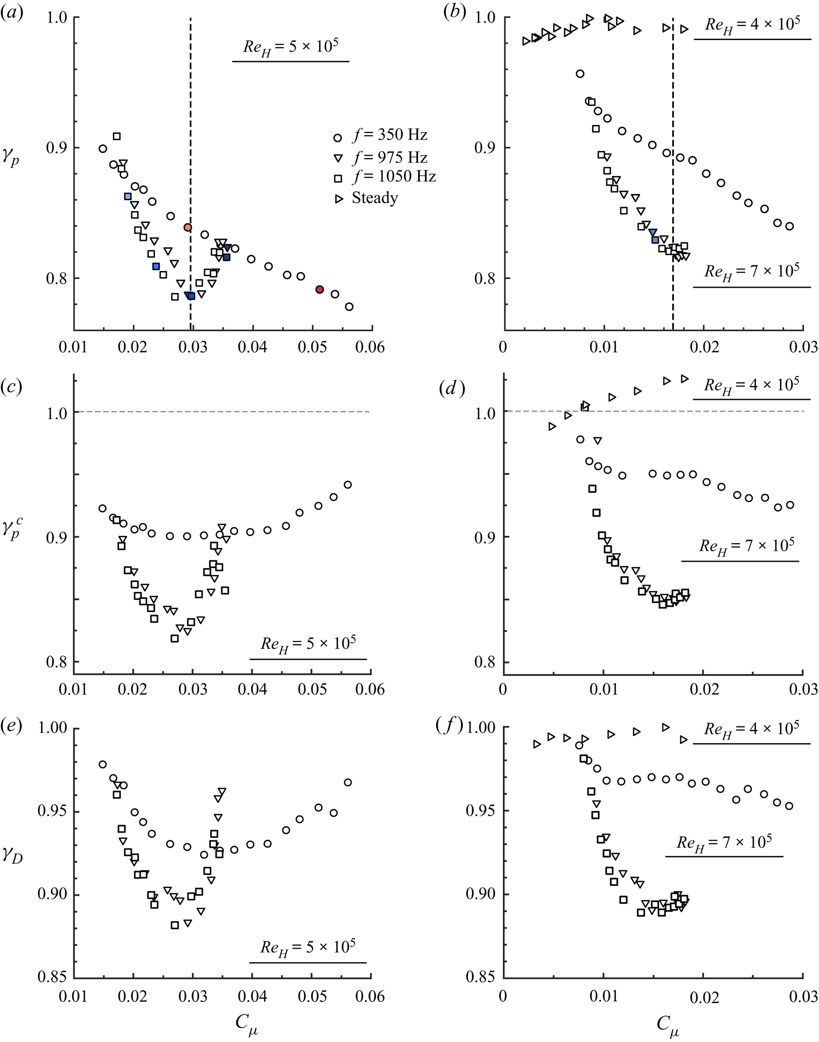
We analyse in figure 3( $a,\!b$) the base pressure changes when the order of magnitude of the forcing frequency is varied at a given free-stream velocity
 $U_0$. From the evolution of
 $\gamma _p$ at both
 $U_0 = 25~\text {m}\,\text {s}^{-1}$ and
 $U_0 = 35~\text {m}\,\text {s}^{-1}$ (corresponding, respectively, to
 $Re_H = 5\times 10^{5}$ and
 $Re_H = 7\times 10^{5}$), there are two main effects of the change in forcing frequency over the chosen range of frequencies: (i) the magnitude of base pressure recovery is strongly dependent on the choice of the forcing frequency
 $f$, and (ii) the trends in the evolution of
 $\gamma _p$ with forcing amplitude
 $C_{\mu }$ are fundamentally different depending on
 $f$.
Evolution of  $(a,\!b)$ the base pressure parameter
 $\gamma _p$,
 $(c,\!d)$ the corrected base pressure parameter
 $\gamma _p^{c}$ and
 $(e,\!f)$ the aerodynamic drag parameter
 $\gamma _D$ with forcing amplitude
 $C_{\mu }$ for the curved surfaces of dimension
 $r = 9h$ at
 $(a,\!c,\!e)$
 $Re_H = 5\times 10^{5}$ and
 $(b,\!d,\!f)$
 $Re_H = 7\times 10^{5}$. Results for steady forcing in
 $(b,\!d,\!f)$ were obtained for
 $Re_H = 4\times 10^{5}$ in order to span a range of forcing amplitudes
 $C_{\mu }$ comparable with those of unsteady forcing. Filled markers are the cases further analysed in § 5 for the detailed description of the drag reduction mechanisms and the unsteady Coanda effect. Vertical dashed lines indicate the
 $C_{\mu }$ at which saturation defined as a minimum in
 $\gamma _p$ occurs.

The first aspect is clearly illustrated by the evolution of  $\gamma _p$ in figure 3
 $(b)$. Steady forcing is found to be inefficient to recover base pressure (
 $\gamma _p$ remains between
 $0.98$ and 1). This is surprising given the established efficiency of steady Coanda blowing for base drag reduction across the literature (Freund & Mungal Reference Freund and Mungal1994; Englar Reference Englar2001; Barros et al. Reference Barros, Borée, Noack, Spohn and Ruiz2016). Nevertheless, it should be pointed out that in the studies of Freund & Mungal (Reference Freund and Mungal1994) and Englar (Reference Englar2001) noticeably higher values of
 $r/h$ or
 $r/H$ are used (
 $r/h$ approximately 50). For unsteady forcing, a notable difference exists at given
 $C_{\mu }$ between forcing at
 $f = 350~\textrm {Hz}$ and at
 $f = 975\text {--}1050~\textrm {Hz}$. Indeed, forcing at
 $f = 1050~\textrm {Hz}$ always produces a greater base pressure recovery in the range of investigated
 $C_{\mu }$. For
 $U_0 = 35~\textrm {m}\,\textrm {s}^{-1}$, the difference culminates at
 $8\,\%$ around
 $C_{\mu } \sim 1.6\times 10^{-2}$. Nevertheless, as made explicit in table 1,
 $f = 350~\textrm {Hz}$ corresponds to
 $St_{\theta }$ of the order of
 $0.02$, which is the most amplified frequency in a free-shear layer (Zaman & Hussain Reference Zaman and Hussain1981). This forcing frequency has been shown to induce base pressure decrease by Oxlade et al. (Reference Oxlade, Morrison, Qubain and Rigas2015) on a bullet-shaped body. Similar conclusions can be drawn from the results at
 $U_0 = 25~\text {m}\,\text {s}^{-1}$ in figure 3
 $(a)$. For this case,
 $f = 350~\textrm {Hz}$ is above the most amplified frequency in the shear layers and thus decoupled from it. At this free-stream velocity, the difference in
 $\gamma _p$ between the two forcing frequencies culminates at
 $6\,\%$ for
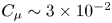 $C_{\mu } \sim 3\times 10^{-2}$.
Nevertheless, for higher  $C_{\mu } \sim 3.6\times 10^{-2}$, there is the beginning of an inversion in terms of base pressure recovery efficiency between both forcings. This point leads to the second aspect introduced previously concerning the difference of trend observed in the evolution of
 $\gamma _p$. Indeed, a clear saturation of the base pressure recovery takes place when forcing at
 $f = 975\text {--}1050~\textrm {Hz}$ starting at
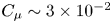 $C_{\mu } \sim 3\times 10^{-2}$ at
 $U_0 = 25~\text {m}\,\text {s}^{-1}$ (respectively,
 $C_{\mu } \sim 1.6\times 10^{-2}$ at
 $U_0 = 35~\text {m}\,\text {s}^{-1}$). Above this threshold, the base pressure recovery is degraded. Such a saturation regime is not found at lower forcing frequency
 $f = 350~\textrm {Hz}$ for which the decrease in
 $\gamma _p$ with
 $C_{\mu }$ is monotonic. This aspect points to the peculiar mechanisms of the unsteady Coanda effect for the highest frequencies investigated, which lead to a higher efficiency in base pressure recovery.
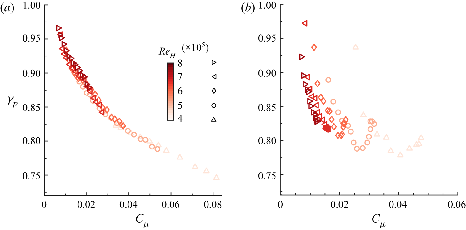
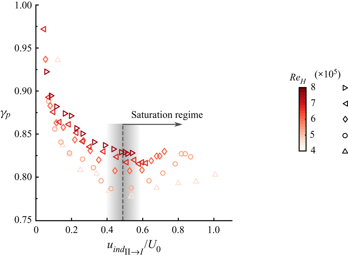
To further investigate this saturation regime at high forcing frequencies, a systematic variation of  $Re_H$ by changing the free-stream velocity
 $U_0$ is operated for forcing at
 $f = 350~\textrm {Hz}$ and
 $f = 975\text {--}1050~\textrm {Hz}$ in order to evidence scaling laws of the base pressure recovery. The evolution of
 $\gamma _p$ presented in figure 4 for
 $Re_H$ in the range
 $(4\text {--}8)\times 10^{5}$ confirms that the amplitude coefficient
 $C_{\mu }$ defined by relation (2.3) is the right scaling parameter to explain the base pressure changes at
 $f = 350~\textrm {Hz}$. Indeed, all the data gathered when forcing at
 $f = 350~\textrm {Hz}$ and varying
 $Re_H$ collapse fairly well onto a single curve in figure 4
 $(a)$. However, the scaling based on the defined
 $C_{\mu }$ completely fails when forcing at higher frequencies (
 $\,f = 975~\textrm {Hz}$ in figure 4b) as the saturation threshold in
 $\gamma _p$ occurs at different
 $C_{\mu }$ depending on
 $Re_H$ and all the curves are horizontally offset. This complete lack of scaling using
 $C_{\mu }$ confirms the evidence of a peculiar mechanism of unsteady Coanda effect at high frequency, quite different from a classical Coanda effect as evidenced at
 $f = 350~\textrm {Hz}$. In § 4, we will propose a scaling parameter to explain this peculiar effect. It is worth mentioning that the conclusions are equivalent when building a momentum coefficient
 $C_{\mu }$ not with the peak jet velocity
 $V_{j_{max}}$ (as also done by Oxlade Reference Oxlade2013) but with the r.m.s. velocity as done by Barros et al. (Reference Barros, Borée, Noack, Spohn and Ruiz2016), for instance. Moreover, Oxlade et al. (Reference Oxlade, Morrison, Qubain and Rigas2015) on an axisymmetric blunt body and Barros et al. (Reference Barros, Borée, Noack, Spohn and Ruiz2016) on an Ahmed body also evidenced such a saturation mechanism in base pressure recovery using simple high-frequency forcing without additional curved surfaces. This mechanism appeared to be governed by the pulsed jet dynamics.
Scaling of the base pressure parameter  $\gamma _p$ variations with forcing amplitude
 $C_{\mu }$ and Reynolds number
 $Re_H$ for curved surfaces of dimension
 $r = 9h$ with forcing at
 $(a)$
 $f = 350~\textrm {Hz}$ and
 $(b)$
 $f = 975~\textrm {Hz}$.

As approximately  $70\,\%$ of the aerodynamic drag of such a body originates from the low-pressure region at the base (Grandemange et al. Reference Grandemange, Gohlke and Cadot2013b; Barros et al. Reference Barros, Borée, Noack, Spohn and Ruiz2016), monitoring the base pressure is a good indicator of the drag changes obtained. Nevertheless, as the curved surfaces are expected to be the location of a low-pressure region due to the local acceleration of the flow and thus to penalize the base pressure recovery obtained, we present in figure 3(c–f) the same evolutions as in figure 3(
 $a,\!b$) but for the base drag parameter
 $\gamma _p^{c}$ (figure 3
 $c,\!d$) and for the aerodynamic drag parameter
 $\gamma _D$ (figure 3
 $e,\!f$) defined in (3.3b,c). Globally, the tendencies in the evolution of
 $\gamma _p^{c}$ and
 $\gamma _D$ confirm the observations made concerning the base pressure parameter
 $\gamma _p$. Maximal drag reduction of
 $12\,\%$ (respectively,
 $11\,\%$) at
 $U_0 = 25~\text {m}\,\text {s}^{-1}$ (respectively,
 $U_0 = 35~\text {m}\,\text {s}^{-1}$) occurs at saturation for the high-frequency forcing at
 $f = 975\text {--}1050~\textrm {Hz}$ and is at least
 $5\,\%$ more important than the drag decrease measured at
 $f = 350~\textrm {Hz}$. The penalization resulting from the low-pressure flow over the curved surfaces is clearly visible from the evolution of
 $\gamma _p^{c}$ in figure 3(
 $c,\!d$). Indeed, on the one hand, the saturation in base drag decrease is even more pronounced at high frequencies than observed on the
 $\gamma _p$ curves with a higher penalization once the saturation threshold
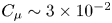 $C_{\mu } \sim 3\times 10^{-2}$ has been exceeded. On the other hand, whereas forcing at
 $f = 350~\textrm {Hz}$ led to a monotonic decrease in
 $\gamma _p$ with
 $C_{\mu }$, it here leads to a saturation in the decrease of
 $\gamma _p^{c}$ above
 $C_{\mu } \sim 2.5\times 10^{-2}$ at
 $U_0 = 25~\text {m}\,\text {s}^{-1}$. Thus the penalization from the curved surfaces cannot be neglected and has to be carefully taken into account in our analysis.
As any active flow control strategy requires input energy in order to work, it is of important practical interest to know whether the developed control strategy is efficient. To assess the energetic performance of our control strategy, we follow energetic analyses discussed in a variety of previous studies (Freund & Mungal Reference Freund and Mungal1994; Choi et al. Reference Choi, Jeon and Kim2008; Barros et al. Reference Barros, Borée, Noack, Spohn and Ruiz2016; Li et al. Reference Li, Borée, Noack, Cordier and Harambat2019). A forcing efficiency can be defined as the ratio between the energy saved by the drag reduction and the mechanical energy of the pulsed jets. For the best case investigated here at  $f = 1050~\textrm {Hz}$ around saturation at
 $U_0 = 35~\textrm {m}\,\textrm {s}^{-1}$, this efficiency ratio is approximately 11. Nevertheless, it should be noted that the forcing apparatus and strategy have not been optimized for energetic efficiency and this aspect remains a key research direction for practical applications, which should be tackled by further studies.
3.2. Unsteady Coanda blowing along curved surfaces: coupling between forcing frequency and radius of curvature
These first observations are here extended by varying the radius of curvature  $r$ of the curved surface by almost halving and doubling the value of the radius (
 $r/h = 9$) previously analysed.
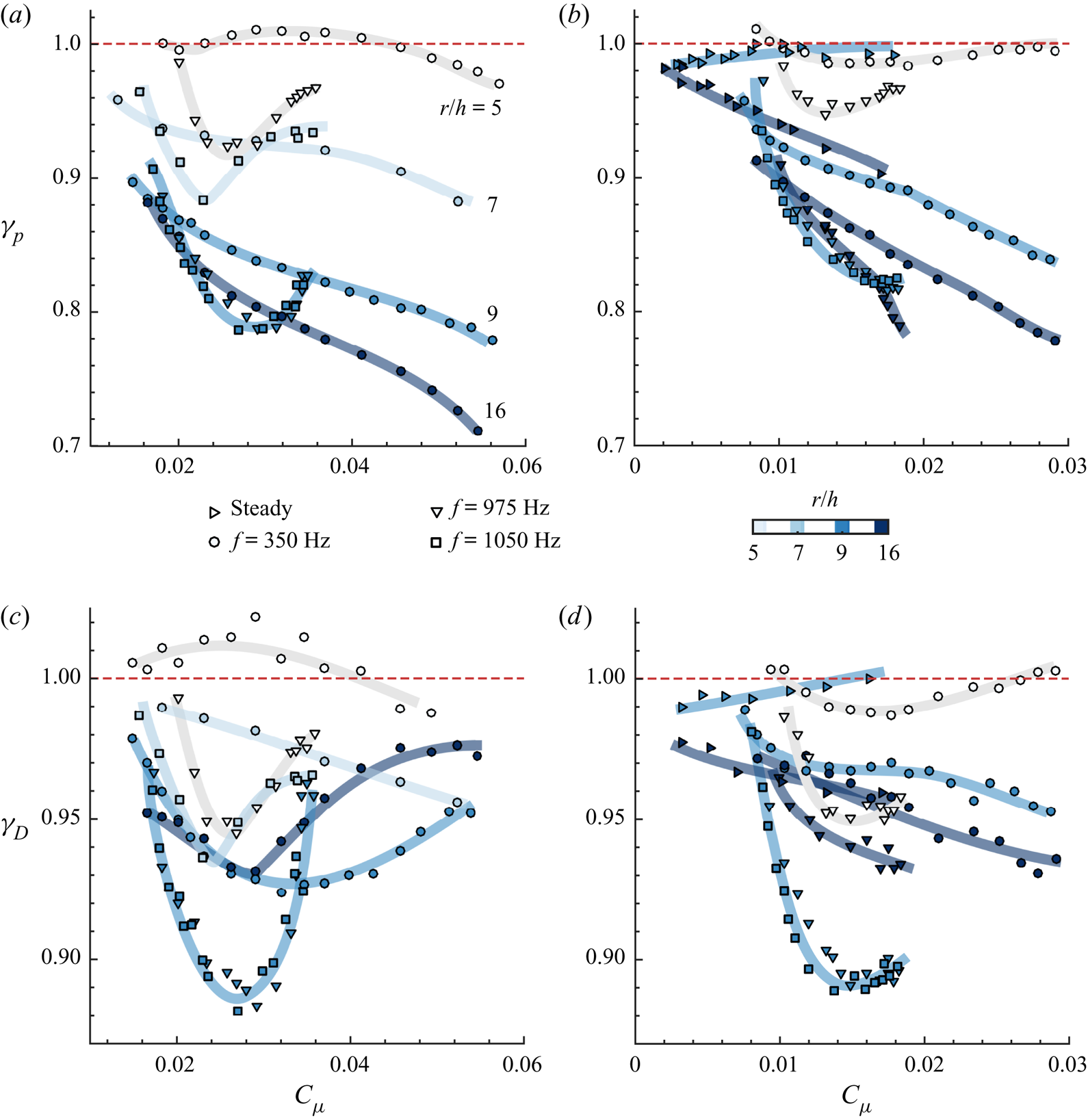
Base pressure and drag reduction depend not only on the forcing amplitude  $C_{\mu }$ but also on the combination of the forcing frequency and the radius of curvature of the curved surfaces. Figure 5 illustrates the rather intriguing evolution of
 $\gamma _p$ and
 $\gamma _D$ for
 $Re = 5\times 10^{5}$ (figure 5
 $a,\!c$) and
 $Re = 7\times 10^{5}$ (figure 5
 $b,\!d$) as function of
 $C_{\mu }$ with
 $r/h$ and
 $f$ as parameters.
Evolution of  $(a,\!b)$ the base pressure parameter
 $\gamma _p$ and
 $(c,\!d)$ the aerodynamic drag parameter
 $\gamma _D$ as a function of the forcing amplitude
 $C_{\mu }$ with variable dimension and radius of curvature
 $r/h = \{5, 7, 9, 16\}$ of the curved surfaces at
 $(a,\!c)$
 $Re_H = 5\times 10^{5}$ and
 $(b,\!d)$
 $Re_H = 7\times 10^{5}$. Markers are coloured according to the radius of curvature
 $r/h$. Similarly to figure 3, results for steady forcing are shown for
 $Re_H = 4\times 10^{5}$ in order to keep forcing amplitudes
 $C_{\mu }$ comparable with those of unsteady forcing. Thick lines give the trend of each set of data in order to highlight the tendency of each curve. Main quantities and qualitative description of the recovery of
 $\gamma _p$ and
 $\gamma _D$ are gathered in table 3.

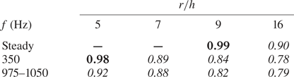
Minimal values of  $\gamma _p$ to illustrate the qualitative efficacy of the Coanda effect to reduce the pressure drag depending on the pair of frequency and radius (
 $\,f$ and
 $r/h$) based on results compiled in figure 5. Italic and bold qualitatively indicate if the pressure drag is (italic) or is not (bold) efficiently reduced by the Coanda effect.

In order to highlight the trends, the tendency of each curve has been qualitatively sketched in thick lines. Table 3 provides a summarized description of the main results of figure 5, the qualitative description for a couple  $(\,f, r/h)$ to succeed – or not – in reducing the pressure drag.
The results gathered in figure 5 emphasize the strong coupling existing between forcing frequency and radius of curvature of the add-ons. Clearly, combinations of  $r/h$ and
 $f$ with a maximum of base pressure recovery and drag decrease exist. Over the range of
 $C_{\mu }$ investigated, higher reduction of
 $\gamma _p$ requires higher forcing frequencies as the radius of curvature decreases. While significant base pressure recovery and drag decrease are obtained at high forcing frequencies even for the smallest radius investigated
 $r/h = 5$ (respectively
 $8\,\%$ and
 $6\,\%$ of base pressure increase and drag decrease on figure 5
 $a,\!c$), it is not the case at the lower forcing frequency
 $f = 350~\textrm {Hz}$ (figure 5
 $a,\!b$ and table 3). Moreover, the steady blowing forcing requires greater radius of curvature to work and to have a clear impact on the drag as drag reduction is only obtained for
 $r/h = 16$. This is globally consistent with previous studies, which mostly focused on steady or pulsed blowing coupled to curved surfaces of greater dimensions
 $r/h > 20$ (Freund & Mungal Reference Freund and Mungal1994; Englar Reference Englar2001; Abramson, Vukasinovic & Glezer Reference Abramson, Vukasinovic and Glezer2011; Lambert et al. Reference Lambert, Vukasinovic and Glezer2019).
For every curved surface radius, the high-frequency forcing always outpasses at a given  $C_{\mu }$ the lower-frequency
 $f = 350~\textrm {Hz}$ forcing both in
 $\gamma _p$ and
 $\gamma _D$ even if for the biggest radius
 $r/h = 16$ the difference in base pressure recovery at a given
 $C_{\mu }$ is reduced (see figure 5b at
 $Re_H = 7\times 10^{5}$).
These differences in pressure drag penalties due to the curved surface underline a difference in the base pressure recovery mechanisms involved. Even if the base pressure recovery is approximately the same for  $r = 9h$ and
 $r = 16h$ (respectively
 $22\,\%$ and
 $25\,\%$ recovery at maximum), the penalization induced by the low-pressure region extending along the curved surface is noticeably higher, resulting in a lower aerodynamic drag decrease (respectively
 $12\,\%$ and
 $7\,\%$ decrease). As the curved surface radius is decreased, the penalization is reduced according to the maximal base pressure recovery and drag decrease observed. For all radii
 $r/h < 16$, the saturation effect persists and occurs at smaller
 $C_{\mu }$ as
 $r/h$ is decreased. Only for
 $r/h = 16$ does the saturation in
 $\gamma _p$ disappear over the investigated range of
 $C_{\mu }$.
3.3. Time scales of the unsteady separation over the curved surface
3.3.1. Role of the jet acceleration time scale
Guided by Van Dyke (Reference Van Dyke1969) and Bradshaw (Reference Bradshaw1973), we can derive the equation for the tangential momentum balance along a mean streamline of the separating wall jet. In order to retain the effects of coherent time fluctuations introduced by the forcing, we perform a phase-averaged decomposition of the flow so that the phase-averaged tangential momentum balance reads:
 \begin{equation} \frac{1}{\rho}\frac{\partial \langle p \rangle}{\partial s} ={-} \frac{\partial\langle U_s \rangle}{\partial t} - \langle U_s \rangle\frac{\partial\langle U_s \rangle}{\partial s} - \frac{\partial\langle u_s'u_s' \rangle}{\partial s} - \frac{\partial\langle u_s'v_n' \rangle}{\partial n} + \text{viscous terms}. \end{equation}
Here, the phase-averaged decomposition of a quantity  $\chi$ with respect to phase
 $t/T$ of the forcing cycle is defined as
 \begin{equation} \langle \chi (\boldsymbol{x},t/T) \rangle = \frac{1}{N}\sum_{n = 0}^{N} \chi(\boldsymbol{x},t/T+n). \end{equation}
The viscous terms are not given explicitly for the sake of simplicity but are kept in the equation in order to perform a time-scale analysis which emphasizes the importance of unsteady effects along the curved surfaces. Two main aspects appear:
(a) On the one hand, if evaluating the viscous diffusion effects in (3.4),
 $\delta = \sqrt {\nu /f}$ allows one to estimate which thickness from the surface is impacted by the viscosity during the forcing cycle. For the typical high-frequency forcing time scales used in our study, $f = 1050~\textrm {Hz}$, $\delta \sim 10^{-4}~\textrm {m}$, which is one order of magnitude smaller than $h$ and two orders of magnitude smaller than $r$. It thus means that viscous diffusion only has time to affect a small thickness of the flow near the curved surface during a forcing period. As a consequence, the flow momentum near the curved surface is higher, preventing the jet from separating from the curved surface under the influence of an adverse pressure gradient imposed by the curvature. This effect explains to some extent the inefficacy of steady blowing when decreasing the curved surface radius ($\delta \sim h/2$ for a Poiseuille flow in this case).
(b) On the other hand, in (3.4), the time derivative of the tangential velocity partly equilibrates the tangential pressure gradient along the curved surface. Given the sign of each quantity, one would expect this term to allow the pulsed wall jet to sustain a stronger adverse pressure gradient along the curved surface during the peaking phase of the forcing cycle. For a positive time derivative of the tangential velocity corresponding to the acceleration phase of the pulsed jet, the adverse pressure gradient along the curved surface diminishes and thus the flow can remain attached farther on the surface. As a consequence, a strong positive tangential acceleration
${\partial \widetilde {U_s}}/{\partial t}$, i.e. small $t_a$ (see table 2), would allow the unsteady Coanda blowing to still work with smaller radius of curvature.


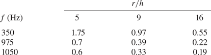
We compare in table 4 for different couples  $(\,f, r/h)$ the ratio between the jet acceleration time scale
 $t_a$ and the characteristic convective time scale related to the curved surface
 $t_{cr} = r/U_0$. This ratio for the configuration (
 $\,f = 350~\textrm {Hz}$,
 $r/h = 5$) is significantly larger than the other values and this configuration was indeed shown to be the only one inefficient in reducing the base drag (see table 3). In this case, the unsteady term may no longer be sufficient for the pulsed jet to sustain the strong adverse pressure gradient along the curved surface, and thus flow detachment over the curved surface is likely to appear and prevent base drag reduction. This comparison of the local convective time scale
 $t_{cr}$ with the pulsed jet acceleration time scale
 $t_a$ allows one to qualitatively predict the occurrence of the Coanda effect indicated in table 3.
Evolution of the ratio  $t_a/t_{cr}$ between the jet acceleration time
 $t_a$ and the local convective time scale
 $t_{cr} = r/U_0$ for the different frequencies and radii of curvature investigated at
 $U_0 = 25~\textrm {m}\,\textrm {s}^{-1}$.

3.3.2. Adaptation of the forcing frequency to the curved surface
To characterize the unsteadiness of the dynamics of flow separation and reattachment over the curved surfaces, we consider now a Strouhal number  $St_r$ based on the convection time scale over the curved surface
 $t_{cr}$:
 \begin{equation} St_r = f t_{cr} = f\frac{r}{U_0}. \end{equation}
This leads to values of  $St_r \sim 0.13$ for
 $f = 350~\textrm {Hz}$ and
 $0.39$ for
 $f = 1050~\textrm {Hz}$. For
 $St_r \sim 1$, the forcing time scale is similar to the characteristic convection time scale over the curved surface. Thus when a new forcing period begins and produces a new pulsed jet, the previous one is still interacting with the curved surface. In this sense the interaction between the curved surface and the pulsed jet is called adapted. When
 $St_r$ is much smaller than one (here, for
 $f = 350~\textrm {Hz}$,
 $St_r = 0.13$), the forcing is unadapted because the flow perturbation from the forcing has sufficient time to be completely convected away from the curved surface before a new forcing period occurs. As a result, the dynamics of the flow over the curved surface becomes more unsteady, with a detrimental impact on the base pressure recovery.
The dynamics of flow reattachment and separation over the curved surface (Waldon etal. Reference Waldon, Peacock, Jacobs, Helu and Haller2008) is investigated in more detail for the two different forcing frequencies of interest with the curved surface  $r/h = 9$. To this purpose, we focus on the spanwise vorticity defined as (for the left-handed system defined in figure 1)
 \begin{equation} \omega_y = \frac{\partial u_x}{\partial z} - \frac{\partial u_z}{\partial x}. \end{equation}
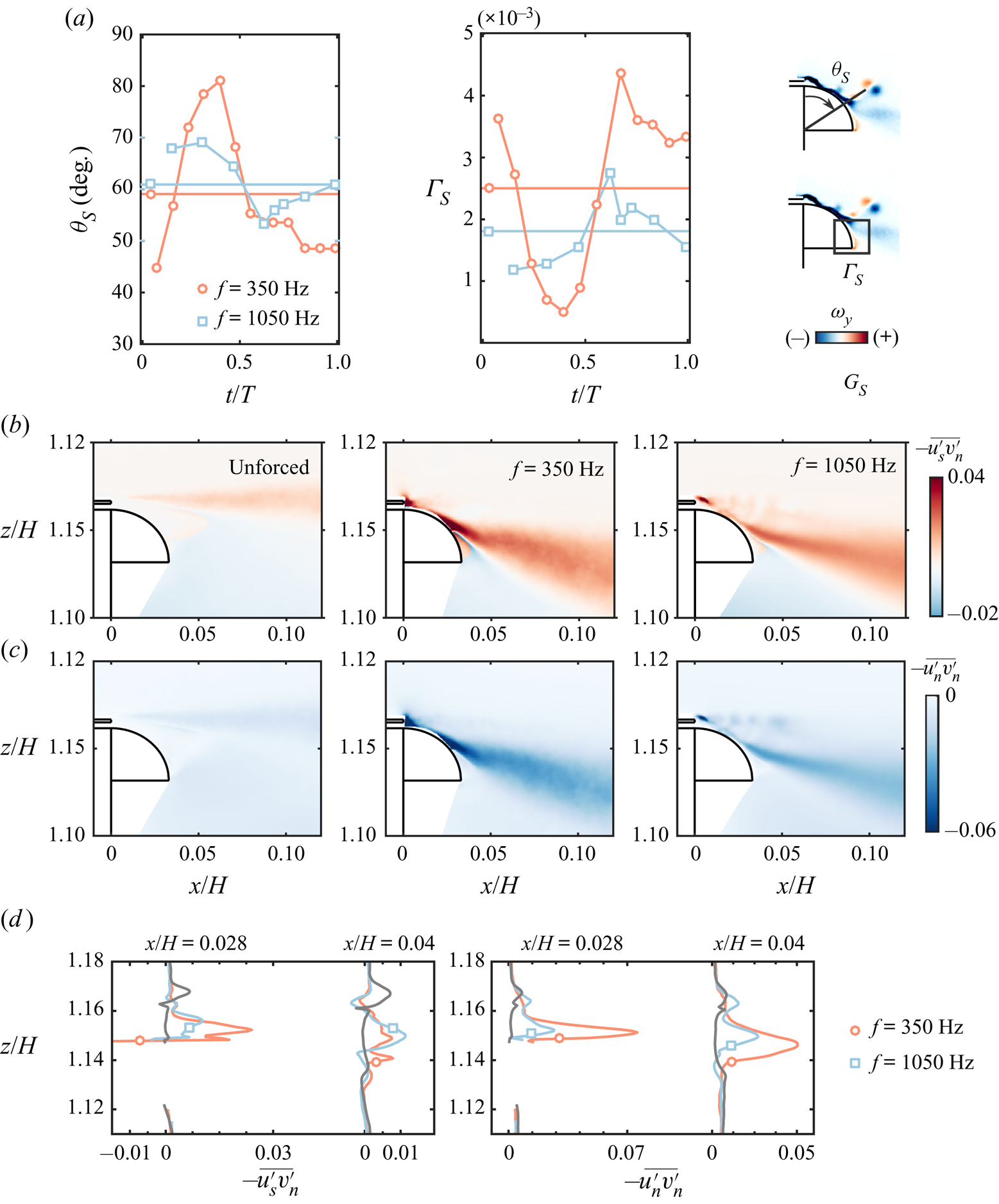
To characterize the evolution of the flow state over the curved surface during one forcing period, we introduce a criterion based on the phase-averaged vorticity  $\langle \omega _y \rangle$ to estimate the location of flow separation on the curved surface. It is defined as the minimal angular position near the curved surface (with origin taken at the slit as indicated on figure 6a) where positive phase-averaged vorticity is found (opposite sign of the vorticity present in the separated shear layer):
 \begin{equation} \theta_S = \min_\theta (\langle \omega_y \rangle \geq 0). \end{equation}
Phase-averaged description of the dynamics of the unsteady reattachment and separation over the curved surface for forcing at  $f = 350~\textrm {Hz}$ and
 $f = 1050~\textrm {Hz}$ at similar forcing amplitude
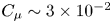 $C_{\mu } \sim 3\times 10^{-2}$ with the
 $r/h = 9$ curved surfaces.
 $(a)$ Phase-averaged evolution of the separation angle
 $\theta _S$ and the positive circulation
 $\Gamma _S$ in the separated region over the curved surface. Horizontal lines denote the time-averaged quantities.
 $(b)$ Tangential–normal Reynolds stresses
 $-\overline {u_s'v'_n}$ and
 $(c)$ normal–normal Reynolds stresses
 $-\overline {v_n'v'_n}$.
 $(d)$ Vertical profiles of Reynolds stresses shown in (
 $b,\!c$) at selected streamwise locations
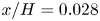 $x/H = 0.028$ (just after the mean location of flow separation from the curved surface) and
 $x/H = 0.04$ (just after the end of the curved surface).

Moreover, to confirm the pertinence of this local criterion, we define a global indicator  $\Gamma _S$ characterizing the strength of the flow separation along the curved surface. It is defined as the total positive circulation in a contour surrounding the detached region over the curved surface (see figure 6a):
 \begin{equation} \Gamma_S = \iint_{C \cap \{\langle \omega_y \rangle \geq 0\}} \langle \omega_y \rangle\,\textrm{d}x\,\textrm{d}z. \end{equation}
The region  $C$ is chosen so as to capture only the positive vorticity induced by the recirculating flow over the downstream part of the curved surface. Indeed, all the positive vorticity originating from the pulsed jets and their interaction with the shear layer is always out of the chosen contour. The separation dynamics presented in figure 6 shows that the mean separation angle
 $\theta _S$ is higher and the mean separation strength
 $\Gamma _S$ is lower for the high-frequency case
 $f = 1050~\textrm {Hz}$ than for the lower-frequency case
 $f = 350~\textrm {Hz}$ at
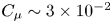 $C_{\mu } \sim 3\times 10^{-2}$ around saturation. Moreover, the lower-frequency forcing at
 $f = 350~\textrm {Hz}$ exhibits stronger fluctuations of both quantities, which accounts for the strong unsteadiness in the reattachment and separation dynamics. This leads to high values of both tangential–normal
 $\overline {u'_sv'_n}$ and normal–normal
 $\overline {v'_nv'_n}$ Reynolds stresses near the curved surface, especially in the vicinity of the mean flow separation from the curved surface, as made explicit in figure 6(
 $b$–
 $d$). A further penalization of the base pressure recovery is thus due to the highly unsteady dynamics of the separation and reattachment process when forcing at
 $f = 350~\textrm {Hz}$.
3.4. Effect of the unsteady reattachment and separation on the surface pressure
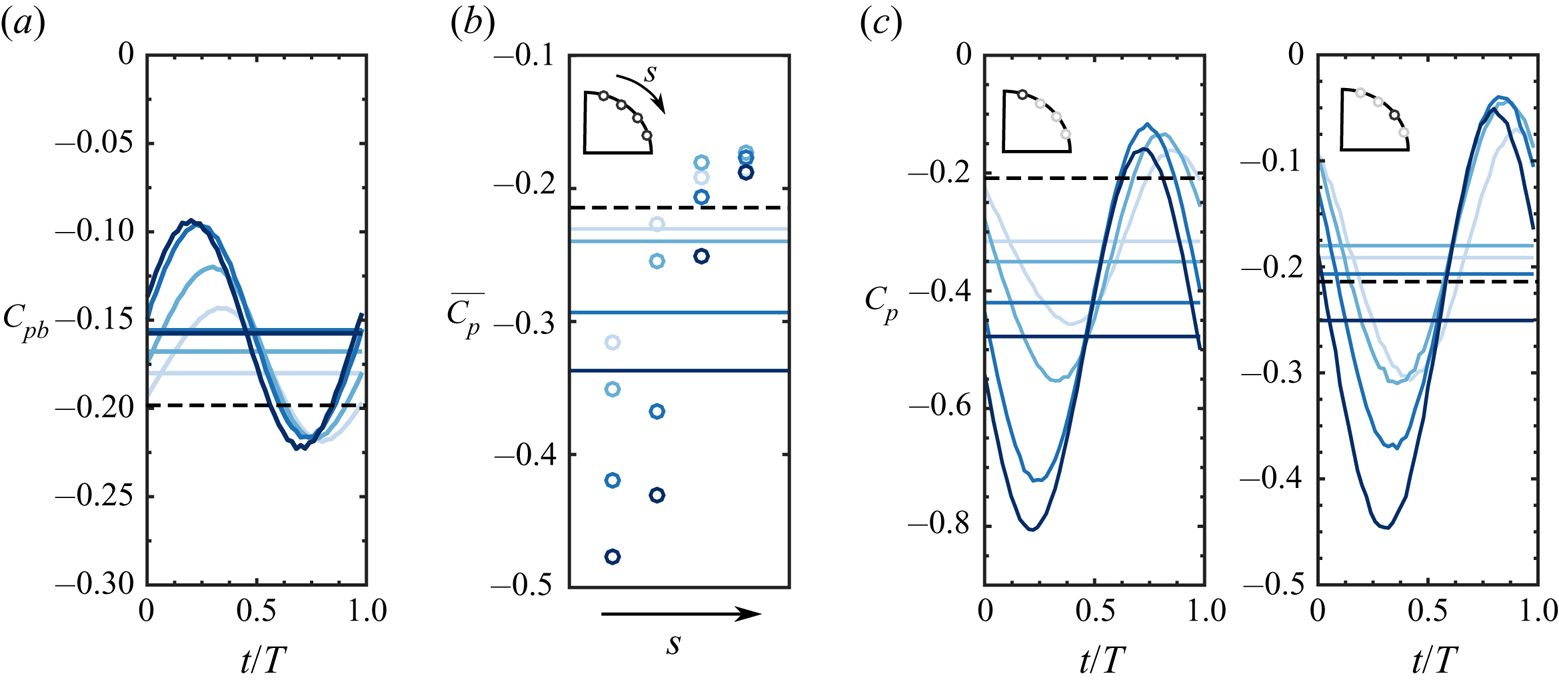
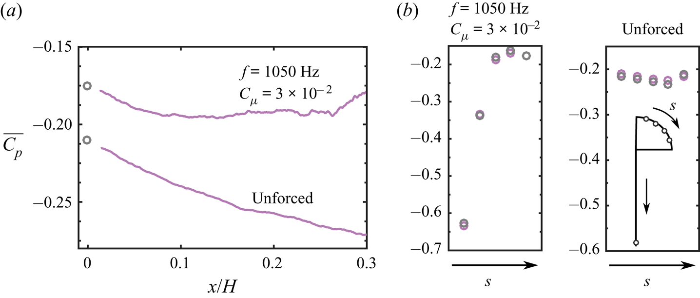
The dynamics of the base pressure  $C_{pb}$ (figure 7a) and the pressure over the curved surface (figure 7c) for forcing at
 $f = 1050~\textrm {Hz}$ for amplitudes
 $C_{\mu } = \{1.9, 2.5, 3, 3.6\}$ spanning the whole investigated range are in complete phase opposition and dictated by the dynamics imposed by the pulsed jets. The evolution of
 $C_{pb}$ indicates that the base pressure recovery is directly related to the importance of the flow reattachment over the curved surface, which dictates the boat-tailing imposed to the wake. A large depression is created over the curved surface during the peaking phase of the pulsed jet velocity followed by an important recompression in the following phase. The amplitude of this recompression can be seen to evolve monotonically with
 $C_{\mu }$ until the saturation with a following decrease at higher
 $C_{\mu }$. This pressure dynamics is completely in line with the flow separation dynamics previously presented in figure 6. Moreover, it should be noted that the pressure dynamics over the curved surface and at the base for forcing at
 $f = 350~\textrm {Hz}$ (not shown here for brevity) follows a similar behaviour as
 $\Gamma _S$ and
 $\theta _S$ with variations of quite large amplitude over a forcing cycle compared with
 $f = 1050~\textrm {Hz}$ (for instance, at the optimum
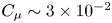 $C_\mu \sim 3\times 10^{-2}$, the base pressure
 $C_{pb}$ undergoes fluctuations of amplitude
 $60 \,\%$ higher at
 $f = 350~\textrm {Hz}$), confirming the difference in adaptation of the pulsed jet/curved surface interaction.
Evolution of the wall pressure coefficient  $C_p$ for forcing at
 $f = 1050~\textrm {Hz}$ with various amplitudes
 $C_{\mu } = \{1.9, 2.5, 3, 3.6\}$. Darker shades of blue indicate increasing forcing amplitude
 $C_{\mu }$.
 $(a)$ Phase-averaged base pressure coefficient
 $C_{pb}$.
 $(b)$ Evolution of the time-averaged pressure coefficient
 $\overline {C_p}$ along the curved surface. Horizontal lines indicate the corresponding mean pressure coefficient averaged along the curved surface
 $\overline {C_{pc}}$.
 $(c)$ Phase-averaged pressure coefficient along the curved surface. Horizontal lines indicate the corresponding time-averaged pressure coefficient
 $\overline {C_p}$. In
 $(c)$ the insets indicate the position of the considered pressure measurement. Horizontal dashed black lines correspond to the unforced flow.

The flow acceleration over the curved surface results in a low-pressure region as expected in the common Coanda effect, which is penalizing the base pressure recovery. This penalization was observed to further increase after the saturation in base pressure recovery at high frequencies of forcing (see figure 3). The average pressure distribution over the curved surface given in figure 7(b) shows the important depression created on the curved surface in the vicinity of the slit. This depression grows with  $C_{\mu }$ and is attenuated when progressing towards the end of the curved surface. It thereby highlights the creation of a low-pressure region whose extent is time-dependent. The first pressure tap considered in figure 7(c) is located upstream of
 $\overline {\theta _S}$ and therefore the local pressure value is below the value of the naturally detached unforced flow. The second pressure tap is located in the vicinity of
 $\overline {\theta _S}$ where the flow detaches. When comparing
 $\overline {C_p}$ at each location with the average pressure distribution over the curved surface in the unforced case, we can see how the flow detaches farther downstream as
 $C_{\mu }$ is increased. This appears very clearly from
 $\overline {C_p}$ being below the unforced average value at the third pressure tap location only for the highest
 $C_{\mu }$ (see figure 7b). This observation accounts for the overly increased penalization induced by the curved surface after the saturation in base pressure recovery.
Now that the main effects of forcing on the pressure drag of the body have been characterized and interpretations of the main time scales governing the unsteady Coanda effect have been introduced, the remainder of the paper focuses on analysing in detail the mechanisms of base drag decrease and trying to build a pertinent model incorporating all the mechanisms behind the unsteady Coanda effect.
4. Scaling the base drag changes: unsteady vorticity dynamics
In this section, an analysis of the unsteady vorticity dynamics driven by the forcing is performed. The aim is to derive a scaling for the base pressure and drag changes observed at high frequency in § 3, able to physically explain the saturation effect.
The following analysis focuses on changes along the top edge of the model, although similar forcing is applied along all four edges of the base. As a matter of generality, the unforced flow conditions along each edge of the model are qualitatively very similar according to the boundary layer measurements of Haffner (Reference Haffner2020). As a consequence, we are confident that the local phenomena discussed here along the top edge can be translated to the other edges of the base. Moreover, Barros et al. (Reference Barros, Ruiz, Borée and Noack2016) provides evidence that the flow behaviour along each edge of the base is qualitatively similar under forcing.
4.1. Local vorticity-flux dynamics at separation
We focus on a fine-scale analysis of the flow interaction with the forcing near the separating edge from a dynamical point of view. This is motivated by the unsteady separation analysis in the previous section having shown the important differences in separation dynamics and their relation to drag changes.
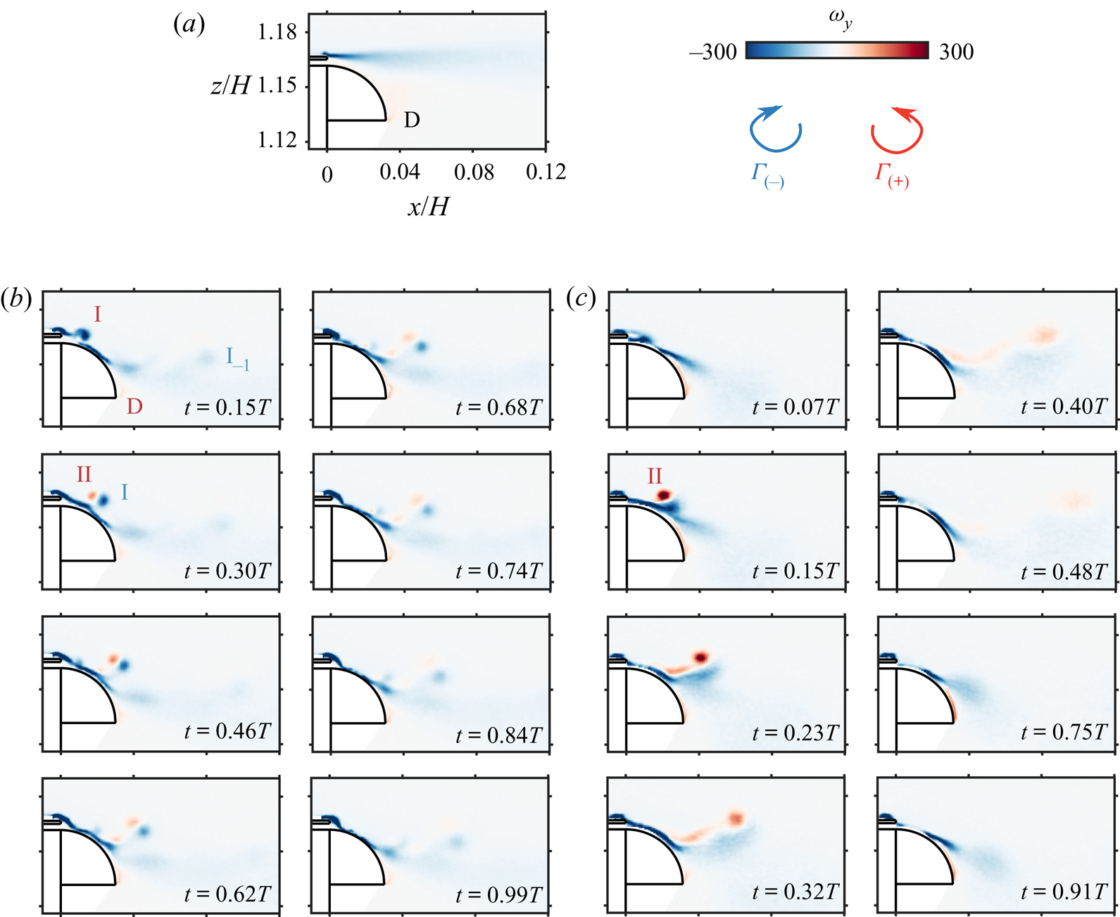
First, it should be noted from the time-averaged spanwise vorticity field depicted in figure 8(a) that the unforced flow is completely detached from the curved surface. This is expected because of the boundary condition imposed at the salient edge over the curved surface. A strong negative vorticity sheet is formed in the continuity of the detachment of the boundary layer at the edge of the base. A weaker positive vorticity sheet is formed from the recirculating flow in the wake interacting with the lower edge of the curved surface (zone denoted D), which was previously used to describe the flow separation dynamics.
Phase-averaged description of the spanwise vorticity  $\omega _y$ dynamics under forcing for the curved surfaces of dimension
 $r = 9h$ at
 $Re_H = 5\times 10^{5}$.
 $(a)$ Time-averaged vorticity
 $\overline {\omega _y}$ of the unforced flow.
 $(b,\!c)$ Phase-averaged vorticity for flow forced
 $(b)$ at
 $f = 1050~\textrm {Hz}$ and
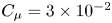 $C_{\mu } = 3\times 10^{-2}$ at times
 $t/T = \{0.15, 0.3, 0.46, 0.62, 0.68, 0.74, 0.84, 0.99\}$, and
 $(c)$ at
 $f = 350~\textrm {Hz}$ and
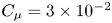 $C_{\mu } = 3\times 10^{-2}$ at times
 $t/T = \{0.07, 0.15, 0.23, 0.32, 0.4, 0.48, 0.75, 0.91\}$. Annotations on the panels correspond to the negative coherent structure forming during the pulsed jet acceleration phase I, the same coherent structure persisting from the previous forcing period (
 $\textrm {I}_{-1}$), the positive coherent structure forming from the pulsed jet II, and the region where the flow is detached from the curved surface (D).

As the pulsed jets are responsible for the modulation of the vorticity flux in the vicinity of separation, the wake dynamics is investigated through a phase-averaged description over the forcing cycle starting at the beginning of the blowing phase. The vorticity dynamics is described in figure 8( $b,\!c$) at
 $Re_H = 5\times 10^{5}$ for the two forcing frequencies
 $f = 350$ and 1050 Hz, both at
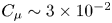 $C_{\mu } \sim 3\times 10^{-2}$, the latter corresponding to the highest base drag reduction case.
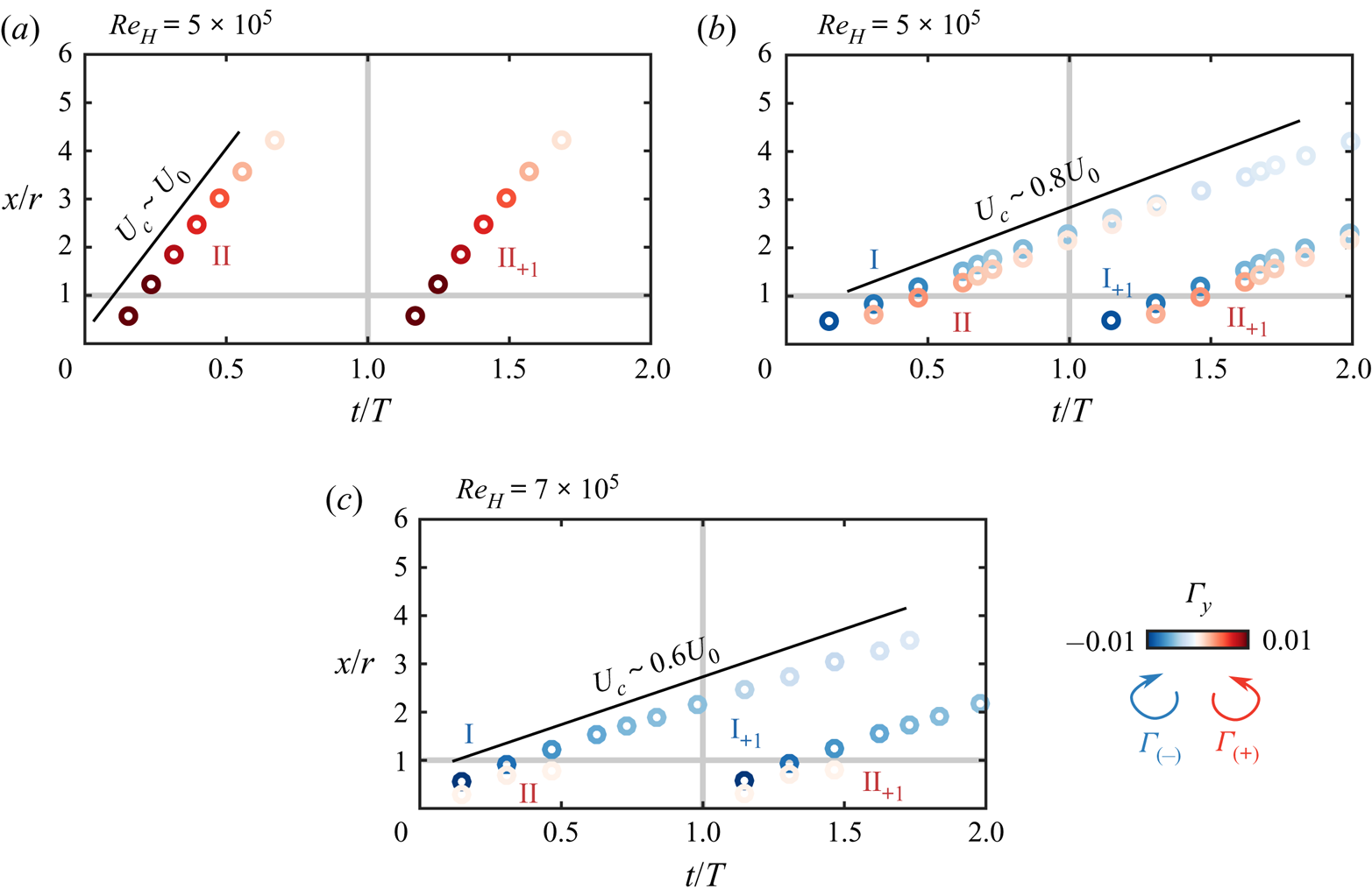
At  $f = 1050~\textrm {Hz}$ (figure 8b), the strong negative vortex sheet is partially attached on the curved surface over a length that can be seen to fluctuate throughout the forcing cycle. The vorticity dynamics during the forcing cycle exhibits the formation of two main coherent structures of opposite vorticity denoted, respectively, I and II. These are convected downstream while interacting with the curved surface and the outer potential flow. The structure with negative vorticity denoted I appears to be formed during the first instants of the forcing cycle (until
 $t/T \sim 0.15$, corresponding to the peaking time of the pulsed jet velocity) by the pinch-off of the separating boundary layer. The vorticity sheet formed at the separation of the boundary layer at the edge of the base is brutally perturbed by the beginning of the blowing phase of the pulsed jets and thus pinches off because of the sudden change in the orientation of separation. It then rolls up to form a structure of apparent size
 $h$. The positive coherent structure II is formed just after I around
 $t/T \sim 0.3$. This positive vorticity coherent structure is likely to originate from the flux of vorticity from the pulsed jet as there is no other source of positive vorticity in the flow (Gharib, Rambod & Shariff Reference Gharib, Rambod and Shariff1998). It is then convected away in a pair with I and they pass over the curved surface where they play a key role in the flow dynamics. At the end of the forcing cycle the two counter-rotating structures have reached approximatively
 $x \sim 2r$ and still remain coherent enough to be detected. Thus, this leads to the formation of a train of coherent structures over a couple of forcing cycles, which is materialized by the structure denoted
 $\textrm {I}_{-1}$, which is the structure I persisting from the previous forcing cycle. This train of coherent structures seems characteristic of this type of high-frequency forcing, as it was already observed through similar measurement techniques by Oxlade et al. (Reference Oxlade, Morrison, Qubain and Rigas2015).
The formation of the negative coherent structure I at the lower frequency of  $f = 350~\textrm {Hz}$ in figure 8(c) does not appear clearly and is more likely absent. Nevertheless, the positive coherent structure II is still formed in a similar fashion. Moreover, as the forcing cycle is three times longer at this forcing frequency, most of the forcing cycle is marked by the absence of coherent structures in the vicinity of the curved surface. This appears as one of the most striking differences with the high-frequency forcing and should consequently affect the interaction with the flow reattachment process over the curved surface.
To further characterize the formation, evolution and convection of these coherent structures I and II, and to analyse their role in the unsteady Coanda effect, we describe their strength by their total circulation  $\Gamma _{\text {I}}$ and
 $\Gamma _{{\text {II}}}$. The circulation of a coherent structure is estimated with the following procedure. The structure is identified using a two-dimensional swirling strength criterion (Zhou et al. Reference Zhou, Adrian, Balachandar and Kendall1999), the threshold of which is chosen high enough to isolate it from the background noise and make the identification unambiguous. Then a rectangular contour
 $C$ is manually drawn around the identified structure to have a supporting contour containing the whole structure where the circulation will be evaluated. (There is only very weak sensitivity of the estimated circulations to the choice of this contour as the vorticity decays rapidly to zero when going away from the centre of the identified region (see figure 17 for instance).) The circulation
 $\Gamma _{\text {I}}$ (respectively,
 $\Gamma _{{\text {II}}}$) is computed as the summation over only negative (respectively, positive) phase-averaged vorticity
 $\langle \omega _y \rangle$:
 \begin{equation} \Gamma_{\text{I}} = \iint_{C \cap \{(x,z);\langle \omega_y \rangle < 0\}} \langle \omega_y \rangle\,\textrm{d}x\,\textrm{d}z ,\quad \Gamma_{{\text{II}}} = \iint_{C \cap \{(x,z);\langle \omega_y \rangle > 0\}} \langle \omega_y \rangle\,\textrm{d}x\,\textrm{d}z. \end{equation}
The position  $\boldsymbol {x}_{\text {I}} = [x_\text {I}, z_\text {I}]$ of the structure I (and analogously for the structure II) is finally evaluated as the barycentre of the identified coherent vorticity:
 \begin{equation} \boldsymbol{x}_{\text{I}} =\frac{{\displaystyle\iint_{C \cap \{(x,z);\langle \omega_y \rangle < 0\}}} \boldsymbol{x} \langle \omega_y \rangle\,\textrm{d}x\,\textrm{d}z} {{\displaystyle\iint_{C \cap \{(x,z);\langle \omega_y \rangle < 0\}} \langle \omega_y \rangle\,\textrm{d}x\,\textrm{d}z}}. \end{equation}
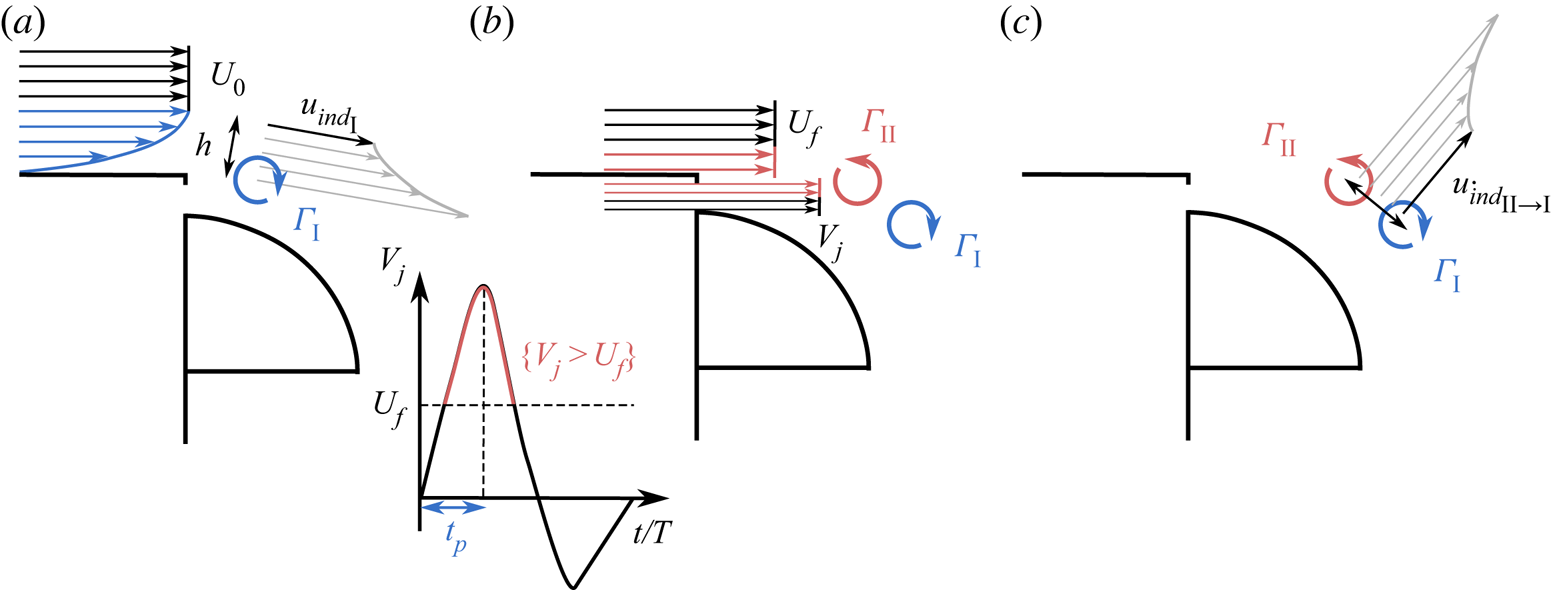
The unsteady flow induced by the pulsed jet over the curved surface leads to the unsteady attachment and separation of the flow and to the mean boat-tailing of the wake. However, the results obtained in this study cannot be completely understood without taking into account the coherent structures I and II. In particular, the structure I, of negative vorticity, induces a downwash velocity downstream. We will show in § 5 that this plays an important role in the curvature of the wake separatrix in the vicinity of the separation from the curved surface. On the contrary, the circulation  $\Gamma _{{\text {II}}}$ of the coherent structure II induces an upward velocity on both the structure I and the flow attached on the curved surface. This may mitigate the positive effect of the structure I and the unsteady attachment. Therefore, we expect this competition to be directly linked to the observed saturation in base pressure recovery.
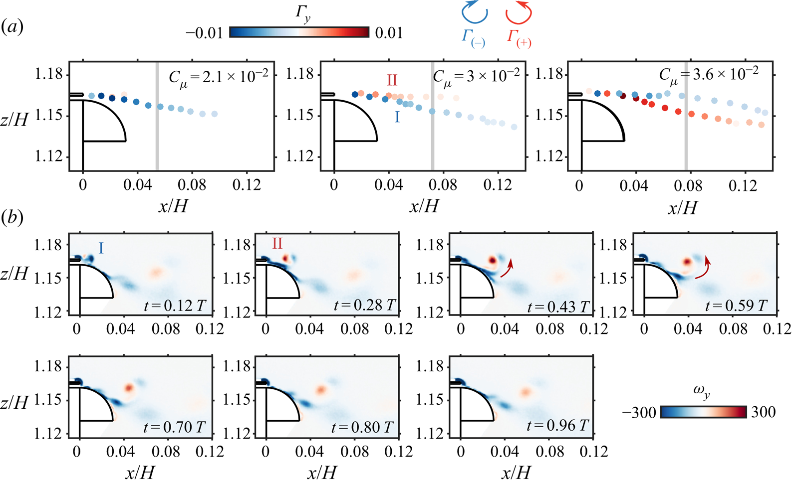
The influence of the structure II when increasing  $C_{\mu }$ above the base pressure saturation threshold appears clearly in figure 9. Indeed, while the trajectory of I remains only moderately influenced by II below
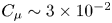 $C_{\mu } \sim 3\times 10^{-2}$ – which can be seen from the undisturbed trajectory of I curving inwards tangentially to the curved surface – its formation and trajectory are strongly disturbed by the presence of structure II above the saturation threshold at
 $C_{\mu } \sim 3.6\times 10^{-2}$. As a consequence, I is entrained by II and has an upwards trajectory towards the end of the curved surface. This lift-off movement is clearly seen from the phase-averaged dynamics detailed in figure 9(b). The global upwards trajectory and rolling-up movement of I induced by II at the end of its formation highlight the dominance of II in the dynamics after saturation.
Circulation dynamics in the base pressure recovery saturation mechanism for forcing at  $f = 1050~\textrm {Hz}$.
 $(a)$ Tracking of the circulation
 $\Gamma$ of the two counter-rotating coherent structures I and II identified in figure 8 when forcing at
 $C_{\mu } = \{2.1, 3, 3.6\}\times 10^{-2}$ at
 $Re_H = 5\times 10^{5}$ for
 $r/h = 9$. Each marker is coloured according to the circulation
 $\Gamma$ of the coherent structure. The vertical grey line indicates the position of I after one period
 $T$ of forcing.
 $(b)$ Phase-averaged sequence of the spanwise vorticity
 $\omega _y$ dynamics for
 $C_{\mu } = 3.6\times 10^{-2}$ after saturation of the base pressure recovery. The red arrows qualitatively illustrate the induced velocity from II entraining I away from the curved surface.

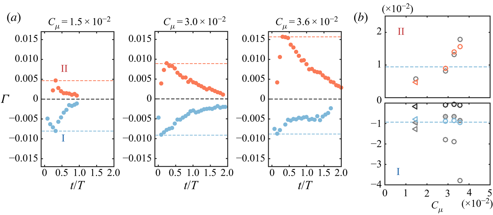
The evolution of the strength of the coherent structures is more finely analysed in figure 10 in order to further describe their origin and formation. The time evolutions of  $\Gamma _{\text {I}}$ and
 $\Gamma _{{\text {II}}}$ are described for forcing at
 $f = 975~\textrm {Hz}$ and varying
 $C_{\mu }$ spanning both below and above saturation regimes (
 $\,f = 975~\textrm {Hz}$ is chosen to take advantage of the more important phases available in our measurements, but the evolutions are qualitatively and quantitatively similar at
 $f = 1050~\textrm {Hz}$). For both structures, in all the cases, a clear distinction can be made between the formation period and the convection and dissipation period. The formation period occurs with a fast time scale for both structures, until maximal absolute circulation has been reached, compared with the dissipation time scale of the structure, which is one order of magnitude longer. Circulation quasi-linearly increases during the formation period before exponential decay occurs during the dissipation of thestructure. Careful examination of the formation times of each structure I and II leads to the following estimations:
(a) Formation of structure I starts at
$t/T = 0$ and lasts a time roughly equivalent to the peaking time $t_p$ of the pulsed jet velocity $V_j$.(b) Formation of structure II starts when
$V_j$ begins to exceed the surrounding flow velocity at the location of formation (of order $U_0$) which allows the vorticity to positively roll up, against the vorticity of the shear layer. Similarly it stops when $V_j$ ceases to exceed the surrounding velocity at the location of formation of order $U_0$.


Evolution and scaling of the circulation  $\Gamma$ of the two counter-rotating structures I and II at
 $f = 975~\textrm {Hz}$.
 $(a)$ Formation and evolution in time for different forcing amplitudes
 $C_{\mu }$. The coloured horizontal dashed lines indicate the approximate maximal circulation reached by each structure.
 $(b)$ Evolution of the peak values of
 $\Gamma$ with
 $C_{\mu }$: experimentally measured
 $\Gamma$ in red and blue, theoretical model of circulation in grey. II: pulsed jet-based circulation from (4.5) in light grey empty symbols. I: boundary layer-based circulation from (4.6) in grey filled symbols, pulsed jet-based circulation from (A 1) in empty light and dark grey symbols (see appendix A for further description). As in figure 4, circles are for
 $Re_H = 5\times 10^{5}$ and left-pointing triangles for
 $Re_H = 7\times 10^{5}$. The horizontal blue dashed lines indicate approximately
 $\pm$ the maximal circulation reached by I.

These time scales are further exemplified in figure 17(a) on a particular example to highlight their accordance with the measured circulation dynamics.
4.2. Scaling the saturation in base pressure recovery
We propose to describe the vorticity dynamics in the vicinity of the separating edge by an inviscid-flow model. The aim is to explain the increased drag reduction observed when forcing at high frequencies of the order of  $O(U_0/r)$ and the concomitant saturation effect at high forcing amplitude
 $C_{\mu }$. Further comments on the scalings on the model introduced in this section are provided in appendix A.
Following Shariff & Leonard (Reference Shariff and Leonard1992) and Berk et al. (Reference Berk, Medjoun and Ganapathisubramani2017), under the local two-dimensional flow assumption, the vorticity flux per unit width can be expressed as
 \begin{equation} \frac{\textrm{d}\Gamma}{\textrm{d}t} = \int \langle \omega_y \rangle \langle u_x \rangle\,\textrm{d}z = \int \frac{\partial \langle u_x \rangle}{\partial z} \langle u_x \rangle\,\textrm{d}z = \frac{1}{2} \langle u_x \rangle ^{2}(t), \end{equation}
with the notation referring to the case of the top shear layer. When further integrating over a period  $t$, the total amount of circulation
 $\Gamma$ created over a given time period is given by
 \begin{equation} \Gamma = \frac{1}{2}\int^{t}_0 \langle u_x \rangle ^{2}\,\textrm{d}t. \end{equation}
As, from the vorticity dynamics described in the previous section, we identified two main coherent structures forming during the forcing cycle, we want to link their formation to the dynamics of the shear layer and the pulsed jets. To do so, figure 11( $a,\!b$) conceptualizes the formation process of the identified counter-rotating structures I and II.
Theoretical inviscid-flow model for the interaction between the pulsed jet and the shear layers surrounding the recirculating wake.  $(a)$ Pinch-off of the separating boundary layer by the pulsed jet during the peaking time
 $t_p$ leading by rolling-up of the boundary layer vorticity to the formation of structure I inducing velocity
 $u_{{ind}_{\text {I}}}$ on the potential region of the wake flow.
 $(b)$ Formation of the counter-rotating structure II during the phase where jet velocity
 $V_j$ exceeds the local surrounding flow velocity
 $U_f$.
 $(c)$ Saturation in base pressure recovery mechanism where the upward velocity induced by II
 $u_{{ind}_{{\text {II}}\to \text {I}}}$ prevents the Coanda effect.

The formation of the structure II is determined by the vorticity flux occurring from the pulsed jet and its interaction with the surrounding flow. It is thus dictated by the difference between the pulsed jet velocity  $V_j$ and a local surrounding flow velocity
 $U_f$ at the location where the structure is formed, in the vicinity of the separating edge. Further insights about this formation velocity are given in appendix A.
Besides, this formation process can only occur if the jet velocity  $V_j$ exceeds
 $U_f$, which is a sine qua non condition for positive circulation to be generated. The time horizon corresponding to this condition is highlighted in red in figure 11(b). It thus leads for the theoretical circulation
 $\Gamma _{{\text {II}}}$ to
 \begin{equation} \Gamma_{{\text{II}}} = \frac{1}{2}\int_{t \in \{t;V_j(t)>U_f\}} (V_j(t)-U_f)^{2}\,\textrm{d}t. \end{equation}
This theoretical circulation estimation is in agreement with the experimentally measured circulation  $\Gamma _{{\text {II}}}$ as shown in figure 10(b).
Structure I forms from the rolling-up of the vorticity of the model's boundary layer. As such, the total circulation  $\Gamma _{\text {I}}$ contained in I is derived from (4.4) and reads as
 \begin{equation} \Gamma_{\text{I}} ={-}\frac{1}{2}\int^{t_p}_0 U_0^{2}\,\textrm{d}t ={-}t_p\frac{U_0^{2}}{2}, \end{equation}
where  $t_p$ is the peaking time of the pulsed jets (the time to reach the maximal jet velocity
 $V_{j_{{max}}}$ as defined in figure 11b) and
 $U_0$ is the free-stream velocity, as the formation process of I involves the vorticity contained in the model's boundary layer at separation. The choice of
 $t_p$ as time horizon for the formation of structure I is physically based on the sudden change in acceleration occurring at the end of the peaking phase. This ends the disruption and roll-up process of the vorticity contained in the boundary layer. It is confirmed by the circulation dynamics analysed in figures 8 and 10 and exemplified on a particular example in figure 17. The physical origin of structure I is validated by the comparison of relation (4.6) with measured circulations in figure 10(b).
The following are two important aspects of these circulation models for  $\Gamma _{\text {I}}$ and
 $\Gamma _{{\text {II}}}$:
(i) the high sensitivity of
$\Gamma _{{\text {II}}}$ to the amplitude of the forcing $C_{\mu }$ contrary to $\Gamma _{\text {I}}$, which remains fairly constant across the investigated configurations; and(ii) the optimality of the pressure drag decrease obtained for values of
$\Gamma _{\text {I}}$ and $\Gamma _{{\text {II}}}$ of similar order of magnitude ($|\Gamma _{\text {I}}| \sim |\Gamma _{{\text {II}}}|$) that appears on figure 10.


As such, the interplay between structures I and II points naturally to a possible mechanism explaining the saturation in pressure drag, which we will further detail.
Using the Biot–Savart law, the velocity induced by structure II on structure I is given by
 \begin{equation} \boldsymbol{u}_{ind_{\text{II}\to\text{I}}} = \frac{\Gamma_{\text{II}}}{2{\rm \pi}}\frac{\boldsymbol{e}_y\times\boldsymbol{d}_{\text{II} \to \text{I}}}{|\boldsymbol{d}_{\text{II}\to \text{I}}|^{2}} \sim \frac{\Gamma_{\text{II}}}{2{\rm \pi}}\frac{\boldsymbol{e}_y\times\boldsymbol{d}_{\text{II} \to \text{I}}}{h^{2}}, \end{equation}
where  $\boldsymbol {d}_{\text {{II}}\to \text {I}}$ is the distance between structures II and I whose norm is of the order of
 $h$. Equation (4.7) holds under the assumption of infinitely long structure II in the spanwise direction, which is relevant according to the very high aspect ratio of the slits from which the pulsed jets emanate and the low
 $Re_h$ value of this rectangular jet flow.
In figure 12 we scale the evolution of the base pressure parameter  $\gamma _p$ with the velocity ratio
 $u_{{ind}_{{\text {II}}\to \text {I}}}/U_0$. All the
 $\gamma _p$ curves for the investigated range of
 $Re_H$ have a saturation collapsing onto a single value of the induced velocity ratio at approximately
 $u_{{ind}_{{\text {II}}\to \text {I}}}/U_0 \sim 0.5$. This confirms that the interaction between the boundary layer and the pulsed jet coherent structures is responsible for the saturation and the pertinence of the model and scaling proposed. The good scaling obtained for the complex interaction between the forcing and the wake flow near separation also justifies a posteriori the approximations made in order to model a local formation velocity
 $U_f$ discussed in (4.5). Moreover, from the obtained scaling, the flow mechanisms involved in the base drag reduction are operating rather differently from what was observed by Barros et al. (Reference Barros, Borée, Noack, Spohn and Ruiz2016) without curved surfaces, where a saturation in base pressure increase was observed at a constant r.m.s. jet velocity at all
 $U_0$, therefore purely dictated by the dynamics of the pulsed jet.
Scaling of the base pressure parameter  $\gamma _p$ variations with the non-dimensionalized induced velocity by structure II on structure I
 $u_{{ind}_{{\text {II}}\to \text {I}}}/U_0$ for the various Reynolds numbers
 $Re_H = \{4,5,6,7,8\}\times 10^{5}$ studied for forcing at
 $f = 975~\textrm {Hz}$ with the curved surface
 $r/h = 9$. The vertical grey shading indicates the approximate constant saturation velocity ratio observed for all
 $Re_H$.

5. Mechanisms of pressure drag decrease: a matter of flow curvature near separation
The peculiar flow mechanism resulting in additional pressure recovery for high-frequency forcing is now scrutinized. As briefly evoked in the previous section, the focus is on a fine-scale analysis of the curvature of the separatrix, which is highly influenced by the identified negative vorticity structure I in the reattachment process.
5.1. Global picture of the wake
The effects of forcing on the wake are first presented from a global viewpoint in figure 13. In figure 13 $(a)$ the focus is directed on a comparison between unforced and forced wakes at both
 $f = 350$ and
 $1050~\textrm {Hz}$ at
 $Re_H = 5\times 10^{5}$ at similar
 $C_{\mu } \sim 3\times 10^{-2}$, around saturation in high-frequency forcing (see figure 3a). Despite a notable difference of
 $6\,\%$ in base pressure recovery between the two forced cases, both wakes remain very similar: the wake separatrix presents a similar shape for both forcings. It is thinner and shorter than the unforced wake, which is qualitatively similar to the observations of Oxlade et al. (Reference Oxlade, Morrison, Qubain and Rigas2015), for instance, on an axisymmetric blunt body. Such a thinner wake is in accordance with the theories of Roshko (Reference Roshko1993) and Sychev et al. (Reference Sychev, Ruban, Sychev and Korolev1998), resulting in a lower momentum deficit and thus increased base pressure as measured. The fact that this shorter wake is associated with base pressure recovery is rather opposite to the conventional relation between increased recirculation length and base pressure recovery found throughout the literature for square-back geometries (Grandemange, Gohlke & Cadot Reference Grandemange, Gohlke and Cadot2013a; Mariotti, Buresti & Salvetti Reference Mariotti, Buresti and Salvetti2015; Lorite-Díez et al. Reference Lorite-Díez, Jimenéz-González, Pastur, Martńez-Bazán and Cadot2020). In this case, there exists a relatively simple relation between the base pressure and the recirculation length
 $L_r$ since the flow curvature can be estimated by the ratio
 $L_r/H$. On the contrary, in the present case, the important local changes in flow curvature around the separation due to the flow reattachment noticeably alter this relation and make it more complex. Nevertheless, no clear distinction between the different forcing frequencies can be made on the basis of a global observation of the wake topology. Furthermore the turbulent fluctuations visualized in figure 13(c) by the turbulent kinetic energy
 $\overline {k} = 0.5 (\overline {u_x'u_x'}+\overline {u_z'u_z'})$ are globally similar in both forced wakes, suggesting a similar activity in the shear layers and flow entrainment in the recirculating wake at a large scale. The pressure field reconstructed from PIV measurements presented in figure 13(b) are consistent with the changes in wake topology, as a recompression throughout the whole wake is observed, resulting in the measured base pressure recovery. It is also worth mentioning that the equilibrium of the wake is fundamentally not affected by the global forcing applied at the base and that the unforced lateral bimodal dynamics persists with qualitatively similar features (Haffner Reference Haffner2020). Thus differences in base pressure are not due to wake asymmetries in the present study.
Global view of the wake.  $(a)$ Wake separatrix for the unforced (black) and for the forced wake at
 $f = 350~\textrm {Hz}$ (red) and
 $f = 1050~\textrm {Hz}$ (blue) at
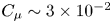 $C_{\mu } \sim 3\times 10^{-2}$. Grey lines represent the projected streamlines in the vertical midplane of the unforced wake.
 $(b)$ Pressure field obtained by direct integration of the momentum equations (see appendix B) with superimposed streamlines for the unforced wake and the wake forced at
 $f = 1050~\textrm {Hz}$ and increasing
 $C_{\mu } = \{2.1, 3, 3.6\}\times 10^{-2}$ (respectively from left to right) at
 $Re_H = 5\times 10^{5}$ for
 $r/h = 9$.
 $(c)$ Mean turbulent kinetic energy
 $\overline {k}$ for the unforced and for the forced wake at
 $f = 350~\textrm {Hz}$ and
 $f = 1050~\textrm {Hz}$ at
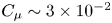 $C_{\mu } \sim 3\times 10^{-2}$.

As no fundamental differences between the two forced wakes emanate from a global point of view of the recirculating wake, our investigation further focuses on the flow differences in the vicinity of separation from the curved surfaces.
5.2. Flow curvature in the vicinity of separation
We build on the theory of Sychev et al. (Reference Sychev, Ruban, Sychev and Korolev1998), which shows the peculiar importance of the curvature of the separatrix around separation to the problem of base pressure generation in the wake of a bluff blunt body. (Trip & Fransson (Reference Trip and Fransson2017) recently experimentally showed the importance of flow curvature around separation on the base pressure of a two-dimensional blunt body.) Following Van Dyke (Reference Van Dyke1969) and Bradshaw (Reference Bradshaw1973), the normal momentum balance along a mean streamline with tangential coordinate  $s$ can be written as
 \begin{equation} \frac{1}{\rho}\frac{\partial \bar{p}}{\partial n} = \kappa\overline{U_s}^{2} - \frac{\partial\overline{u_s'v_n'}}{\partial s} - \frac{\partial\overline{v_n'v_n'}}{\partial n}, \end{equation}
where  $n$ is the coordinate along an axis locally normal to the streamline and
 $\kappa = \text {det}(\boldsymbol {x}',\boldsymbol {x}'')/\|\boldsymbol {x}'\|^{3}$ is the local streamline curvature, with
 $\boldsymbol {x} (s) = (x(s),z(s))$. Equation (5.1) is of fundamental interest in analysing the normal pressure gradient across the wake separatrix, which allows one to interpret the pressure changes in the recirculating wake and near the base. The normal gradient of normal velocity fluctuations
 $\partial \overline {v_n'v_n'}/\partial n$ in (5.1) can be neglected in our first-order analysis: it is one order of magnitude smaller than the curvature term for forced cases and it acts only by locally generating a low-pressure region inside the shear layer without contributing notably to the pressure gradient across the separatrix on large scales. Moreover, the tangential gradient of normal–tangential velocity fluctuations
 $\partial \overline {u_s'v_n'}/\partial s$ appears also as one order of magnitude smaller than the curvature term after careful investigation (not detailed here for brevity).
We therefore first focus on the curvature term  $\kappa \overline {U_s}^{2}$, which is preponderant in establishing the pressure gradient, and analyse the simplified balance of (5.1) on the separatrix near the curved surface in figure 14. To this purpose, a series of five adjacent mean streamlines are chosen as exemplified in figure 14(a) to scrutinize the curvature effects. Streamlines originate around a location
 $z \sim G+H+\theta$, thus one momentum thickness above the trailing edge. The local curvature of each streamline is estimated from the PIV measurements and results are averaged across all streamlines to reduce the influence of measurement noise in the second-order spatial derivatives required by the curvature estimation. The separatrices of the analysed cases are depicted in figure 14(b). For all the forcing cases, the separatrix is importantly deviated inwards compared with the unforced separatrix. This results in a lowered momentum deficit in the wake, and therefore a wake recompression and base pressure recovery as a regular boat-tailing effect would do. Nevertheless, the separatrices with the higher deflection angles at the end of the considered region, for forcing at
 $f = 350~\textrm {Hz}$ and
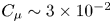 $C_{\mu } \sim 3\times 10^{-2}$ and for forcing at
 $f = 1050~\textrm {Hz}$ and
 $C_{\mu } \sim 3.6\times 10^{-2}$, are not those resulting in the highest base pressure recovery or equivalently lowest base drag. Indeed, for forcing conditions around the saturation (
 $\,f = 1050~\textrm {Hz}$ and
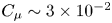 $C_{\mu } \sim 3\times 10^{-2}$), even if the deflection angle is less important at the end of the region of interest, the separatrix exhibits greater curvature in the vicinity of the curved surface. This is further assessed through the tangential evolution of the curvature term of the normal pressure gradient
 $\kappa \overline {U_s}^{2}$ in figure 14(c).
Streamwise evolution along the separating streamline of the normal pressure gradient  ${\partial p}/{\partial n}$ related to curvature obtained from (5.1).
 $(a)$ Example of an ensemble of five streamlines originating at approximately
 $z \sim G+H+\theta$ used for averaging the curvature
 $\kappa$ and the normal pressure gradient
 ${\partial p}/{\partial n}$ estimation.
 $(b)$ Separating streamlines originating from the same point for unforced and various forced cases. The colours are defined the same as in
 $(c)$.
 $(c)$ Streamwise evolution of the normal pressure gradient estimated from the curvature part of (5.1) for forcing at
 $f = 350~\textrm {Hz}$ and
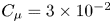 $C_{\mu } = 3\times 10^{-2}$, and at
 $f = 1050~\textrm {Hz}$ and
 $C_{\mu } = \{1.9, 2.5, 3, 3.6\}$. The unforced case is additionally shown in black in the first graph. Thin vertical grey lines indicate the streamwise extent of the curved surface.

When forcing is applied, an important peak in the term can be seen around the end of the curved surface at  $x/H \sim 0.04$, corresponding to a local curvature inversion due to the presence of an inflection point in the separatrix. Such a curvature inversion is interpreted through (5.1) as a local inversion of the normal pressure gradient across the separatrix and thus as leading to a recompression inside the recirculating wake region and base pressure recovery. Around the saturation in base pressure recovery at
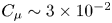 $C_{\mu } \sim 3\times 10^{-2}$ the peak in curvature is notably higher at
 $f = 1050~\textrm {Hz}$ than at
 $f = 350~\textrm {Hz}$, approximately
 $30\,\%$ more, which explains the observed difference in base pressure recovery. Conversely at
 $f = 1050~\textrm {Hz}$, the peak of curvature is seen to increase monotonically with
 $C_{\mu }$ until the saturation in base pressure is reached before this amplitude collapses, being thus in line with the measured base pressure changes. The maxima of the curvature term
 $\max _s(\kappa \overline {U_s}^{2})$ and the averaged curvature over the region where curvature is reversed
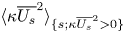 $\langle \kappa \overline {U_s}^{2} \rangle _{\{s;\kappa \overline {U_s}^{2} > 0\}}$ for the different forcing conditions are gathered in table 5 to confirm our reasoning. These curvature changes implied by the induced velocity effects discussed previously are therefore the supplemental mechanism behind the unsteady Coanda effect allowing for further base pressure recovery. These peculiar curvature inversion changes complement the other known effect of wake thinning seen from the inward deviation of the separatrix in the base pressure recovery mechanism.
Quantitative characteristics of the curvature inversion. Extreme values of  $\kappa \overline {U_s}^{2}$ and spatial average value
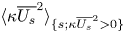 $\langle \kappa \overline {U_s}^{2} \rangle _{\{s;\kappa \overline {U_s}^{2} > 0\}}$ where the sign of the quantity is reversed corresponding to the curvature inversion region.

To further augment and confirm our curvature analysis from the use of (5.1), we show in figures 15 and 16 the pressure fields obtained by direct integration of the momentum equations from the PIV velocity fields. The method is briefly described and carefully validated in appendix B. The effect of forcing frequency at 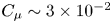 $C_{\mu } \sim 3\times 10^{-2}$ around saturation is first exposed in figure 15. Two main observations can be made for both forcings based on these
 $\overline {C_p}$ fields:
(a) A region of strong depression is formed around the trailing edge due to the local acceleration of the flow, which extends over the curved surface, thus penalizing the aerodynamic drag reduction, as confirmed by the pressure measurements on the curved surface.
(b) A global recompression takes place in the wake, which extends by continuity to the pressure at the base of the model.
Mean pressure coefficient  $\overline {C_p}$ obtained by integration of the momentum equations in the
 $(x,z)$ plane.
 $(a)$ The
 $\overline {C_p}$ fields for unforced, and
 $f = 350$ and
 $1050~\textrm {Hz}$ at similar forcing amplitude
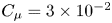 $C_{\mu } = 3\times 10^{-2}$ around the saturation in base pressure recovery at
 $Re_H = 5\times 10^{5}$ with the
 $r/h = 9$ curved surfaces. The blue shades colour map allows for scrutinizing the very-low-pressure region near the separating edge when forcing.
 $(b)$ The corresponding
 $\overline {C_p}$ vertical profiles at different streamwise locations
 $x/H = \{0.04, 0.1, 0.2, 0.3\}$. The mean separating streamlines are given in grey, and black vertical dashed lines in the first field give the streamwise position of the profiles plotted in
 $(b)$.

Effect of forcing amplitude on the mean pressure coefficient  $\overline {C_p}$ obtained by integration of the momentum equations in the
 $(x,z)$ plane.
 $(a)$ The
 $\overline {C_p}$ fields for
 $f = 1050~\textrm {Hz}$ at
 $C_{\mu } = \{2.5,3,3.6\}\times 10^{-2}$ around the saturation in base pressure recovery at
 $Re_H = 5\times 10^{5}$ with the
 $r/h = 9$ curved surfaces. The blue shades colour map allows for scrutinizing the very-low-pressure region near the separating edge when forcing.
 $(b)$ The corresponding
 $\overline {C_p}$ vertical profiles at different streamwise locations
 $x/H = \{0.04, 0.1, 0.2, 0.3\}$. The mean separating streamlines are given in grey.

The region of strong depression can be seen to extend farther at  $f = 350~\textrm {Hz}$, which is clearly quantified by the vertical pressure profiles at
 $x/H = 0.04$. This explains the further penalization at these unadapted frequencies for this choice of
 $r/h$ and the advantage given by the unsteady Coanda effect. A low-pressure trace at
 $f = 1050~\textrm {Hz}$ in the flow can be identified, coinciding with the trajectory of the coherent structures I and II formed by the forcing at high frequency, as was also observed by Oxlade et al. (Reference Oxlade, Morrison, Qubain and Rigas2015). On the wake side of the separatrix, locally around the end of the curved surface, the recompression in the flow is more important at
 $f = 1050~\textrm {Hz}$. This is visible in particular from the vertical profile at
 $x/H = 0.04$ at the end of the curved surface in figure 15(b), where very locally below the separatrix the pressure is further increased to its highest value and by continuity spreading in the wake then. This location coincides with the location of the peak in curvature presented in figure 14, which confirms the peculiar effect of flow curvature in the unsteady Coanda effect for obtaining further drag decrease. Finally, when looking at high forcing frequency
 $f = 1050~\textrm {Hz}$ for increasing
 $C_{\mu }$ in figure 16, the depression around the trailing edge can be seen to increase monotonically with
 $C_{\mu }$ whereas the recompression on the wake side saturates for
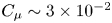 $C_{\mu } \sim 3\times 10^{-2}$ to weaken when further increasing the forcing amplitude. This further highlights the advantage of flow curvature resulting from the unsteady Coanda effect in producing a recompression of the wake without important penalties on the contrary of a common inwards flow deviation which induced strong penalization from the low-pressure region extending over the curved surface.
5.3. An inviscid-flow model to evaluate frequency–radius coupling effects
As was stated in the previous section, the flow curvature just after separation is the key mechanism explaining the differences in base drag changes. We thus seek to relate these additional curvature changes to the coherent circulation dynamics previously described. This is done by further developing the inviscid-flow model previously introduced with the aim of taking into account the frequency–radius coupling in the unsteady Coanda effect.
Inspired by the study of Berk & Ganapathisubramani (Reference Berk and Ganapathisubramani2019) about the induced velocity effects of a pulsed jet in a cross-flow using an inviscid-flow model, the model from § 4 is further refined to describe the influence of the coherent circulation dynamics on the wake separatrix. To this purpose, the inviscid-flow model from (4.5), (4.6) and (4.7) is extended to characterize the flow induced by the peculiar coherent structures at high- $St_r$ forcing. Figure 17
 $(a,\!b)$ shows the ingredients of this extended model on one peculiar case, which is chosen to be the forcing at
 $f = 1050~\textrm {Hz}$ (
 $St_r \sim 0.39$) around the saturation where the base drag decrease is maximal. The measured time evolutions of the circulation of structures I and II are fitted with a physical model building on the approach of (4.6) and (4.5) (full lines in figure 17a):
 \begin{equation} \Gamma_{\text{I}}(t) = \begin{cases} \dfrac{t}{t_p}\Gamma_{\text{I}_0}\exp\left(-\dfrac{t_p}{\tau_{\text{I}}}\right), & t < t_p, \\ \Gamma_{\text{I}_0}\exp\left(-\dfrac{t}{\tau_{\text{I}}}\right), & t>t_p, \end{cases} \end{equation}
and
 \begin{equation} \Gamma_{{\text{II}}}(t) = \begin{cases} 0, & t < t_{{\textit{min}}_{{\text{II}}}}, \\ \dfrac{t-t_{{min}_{{\text{II}}}}}{t_{{\textit{max}}_{{\text{II}}}}-t_{{\textit{min}}_{{\text{II}}}}}\Gamma_{{\text{II}}_0}\exp\left(-\dfrac{t_{{\textit{max}}_{{\text{II}}}}}{\tau_{{\text{II}}}}\right), & t_{{\textit{min}}_{{\text{II}}}} < t < t_{{\textit{max}}_{{\text{II}}}},\\ \Gamma_{{\text{II}}_0}\exp\left(-\dfrac{t}{\tau_{{\text{II}}}}\right), & t>t_{{\textit{max}}_{{\text{II}}}}. \end{cases} \end{equation}
Here  $t_{{min}_{{\text {II}}}} = \min _t\{t;V_j(t)>U_f\}$,
 $t_{{max}_{{\text {II}}}} = \max _t\{t;V_j(t)>U_f\}$ and
 $\Gamma _{\text {I}_0}$ (
 ${<}0$),
 $\tau _{\text {I}}$,
 $\Gamma _{{\text {II}}_0}$ (
 ${>}0$) and
 $\tau _{{\text {II}}}$ are the fitting parameters of the model. Each time evolution of the circulation is based on a linear increase of
 $\Gamma$ during the formation period, followed by an exponential decay primarily dictated by the dissipation of the coherent structures. If assuming a constant
 $t_p/T$ in concordance with our HWA measurements on the pulsed jets,
 $t_{{min}_{{\text {II}}}}/T$ and
 $t_{{max}_{{\text {II}}}}/T$ are also constant and it allows for a forcing frequency parametrization of the model with a circulation
 $\Gamma$ scaling as
 $T$.
Inviscid model for the velocity induced by the identified coherent structures.  $(a)$ Fitting of the temporal evolution of the circulation
 $\Gamma$ of counter-rotating coherent structures I and II for the case of optimal base pressure recovery at
 $f = 1050~\textrm {Hz}$ (
 $St_r \sim 0.39$) and
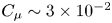 $C_{\mu } \sim 3\times 10^{-2}$. Squares are experimental results, and full lines the fit to these points from (5.2) and (5.3).
 $(b)$ Fitting of the spatial evolution of the spanwise vorticity
 $\omega _y$ of counter-rotating coherent structures I and II. Squares are experimental results, and full lines the fit to these points from (5.4) describing a Lamb–Oseen vortex.
 $(c)$ Example of spanwise vorticity
 $\omega _y$ (top) and induced vertical velocity
 $u_z^{{ind}}$ (bottom) fields at a given time instant of the forcing cycle obtained from the inviscid model. The vorticity field includes the vorticity images inside the curved surface.

In a similar way, the evolution of the position of the centre of the coherent structures  $\boldsymbol {x_{\text {I}}}$ and
 $\boldsymbol {x_{{\text {II}}}}$ is fitted with linear time evolutions as appeared from the constant convection velocities estimated in figure 20. Using the modelled circulation, the associated spatial distribution of vorticity is accurately approximated by that of a Gaussian or Lamb–Oseen vortex, which gives for structure I, for instance,
 \begin{equation} \omega_{y_\text{I}}(\boldsymbol{x},t) = \frac{\Gamma_{\text{I}}(t)}{{\rm \pi} |\boldsymbol{x}-\boldsymbol{x}_{\text{I}}|^{2}} \exp \left(-\frac{|\boldsymbol{x}-\boldsymbol{x}_{\text{I}}|^{2}}{r_{\text{I}}(t)^{2}}\right). \end{equation}
Here  $r_{\text {I}}$ is the radius of structure I given as a fitting parameter from the measurements whose evolution during time can be approximated as constant and of the order of
 $h$ (thereby justifying the exponential decay of circulation completely dominated by dissipation over diffusion). An example of the experimentally measured vorticity compared with the model of (5.4) for one time instant is given in figure 17(c) confirming the pertinence of the model. The total vorticity field
 $\omega _y(\boldsymbol {x},t)$ of the train of coherent structures identified is then the sum of the vorticity distribution from all structures I and II and their equivalent from previous forcing periods.
In order to satisfy the no-penetration condition on the curved surface, for each external vorticity source at a location  $\boldsymbol {x}_S$, an image vortex of equal but opposite circulation is located at the inverse square point
 $\boldsymbol {x}_S'$ defined as
 $(\boldsymbol {x}_S-\boldsymbol {x}_C) \boldsymbol {\cdot } (\boldsymbol {x}_S'-\boldsymbol {x}_C) = r^{2}$, where
 $\boldsymbol {x}_C$ is the centre of the circle defining the curved surface. Finally, a vortex of equal circulation to each of the external vorticity source is located at
 $\boldsymbol {x_C}$ to cancel the total circulation of the internal vorticity sources of the images (Saffman Reference Saffman1992; Pitt Ford & Babinsky Reference Pitt Ford and Babinsky2013). An example of the total vorticity field obtained at a given time instant is provided in figure 17(c).
As discussed by Berk & Ganapathisubramani (Reference Berk and Ganapathisubramani2019), the associated induced velocity field is then obtained by application of the Biot–Savart law
 \begin{equation} \boldsymbol{u}{}^{{ind}}(\boldsymbol{x},t) = \iint \frac{\omega_y(x',z',t)}{2{\rm \pi}\max(|\boldsymbol{x}'-\boldsymbol{x}|,r_R)} \frac{\boldsymbol{e}_y\times(\boldsymbol{x}'-\boldsymbol{x})} {|\boldsymbol{x}'-\boldsymbol{x}|}\,\textrm{d}x'\,\textrm{d}z' . \end{equation}
Here the summation is performed over the vorticity contributions from each location  $(\textrm {d}x',\textrm {d}z')$ of the field; and
 $r_R$ is an equivalent Rankine vortex radius used to keep a finite velocity everywhere in the field and which is empirically chosen as
 $\sqrt {(0.5\,\textrm {d}x')^{2}+(0.5\,\textrm {d}z')^{2}}$ related to the field pitch. An example of the induced velocity field
 $\boldsymbol {u}^{{ind}}(\boldsymbol {x},t)$ thus computed is given in figure 17
 $(c)$.
It should be noted here that the proposed model is also implicitly parametrized in forcing frequency through the time dependence in relations (5.2) and (5.3). Indeed, the peak in circulations  $|\Gamma _{\text {I}}|$ and
 $|\Gamma _{{\text {II}}}|$ will by definition theoretically scale with
 $1/f$ (Shariff & Leonard Reference Shariff and Leonard1992; Berk & Ganapathisubramani Reference Berk and Ganapathisubramani2019). In addition, as all the formation time parameters in relations (5.2) and (5.3) are expressed relative to the forcing period duration
 $T$, the assumption is then that the time evolution of circulation is homothetic when frequency is varied in the model. This is in line with the properties of our pulsed jets discussed in § 2.5. Indeed, the time evolution of the pulsed jet velocity is close to homothetic at the investigated forcing frequencies, with constant duty cycle used, and near-constant non-dimensional peaking time
 $t_p/T$. As a consequence, the inviscid-flow model discussed herein and built on the experimental results of the optimal base drag decrease (
 $\,f = 1050~\textrm {Hz}$ and
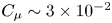 $C_{\mu } \sim 3\times 10^{-2}$) can be reasonably used to at least qualitatively investigate the forcing frequency effects on the velocity induced by the coherent structures.
To analyse the influence of these coherent structures on the mean flow in the vicinity of the curved surface, we examine the mean vertical induced velocity  $\overline {u_z^{{ind}}}$ in figure 18. The
 $\overline {u_z^{{ind}}}$ field at
 $f = 1050~\textrm {Hz}$ (
 $St_r = 0.39$) exhibits two distinct zones with opposite velocities: a region near the slit and the curved surface with positive
 $\overline {u_z^{{ind}}}$, followed by a region with negative
 $\overline {u_z^{{ind}}}$. The latter region contributes to the flow deviation and to the curvature of the wake separatrix that lead to an additional base pressure recovery. To quantify the importance of this influence, the induced vertical velocity is approximately one-fifth of the vertical velocity measured by the PIV in the same region. This mean negative vertical induced velocity only appears farther downstream (
 $x/r > 2$) when forcing at
 $f = 350~\textrm {Hz}$ (
 $St_r = 0.13$) and the vicinity of the curved surface is characterized by the presence of positive vertical induced velocity.
Inviscid model for the velocity induced by the identified coherent structures.  $(a)$ Time-averaged vertical induced velocity
 $\overline {u_z^{{ind}}}$ for the nominal case
 $St_r = 0.39$ and for lower (
 $St_r = 0.13$) and higher (
 $St_r = 0.78$ and
 $St_r = 1.17$) frequencies.
 $(b)$ Time-averaged induced vertical velocity
 $\overline {u_z^{{ind}}}$ on a line originating at the trailing edge and following the mean direction of convection of the coherent structures (depicted in
 $(a)$) for various forcing frequencies
 $St_r = \{0.04, 0.13, 0.26, 0.39, 0.78, 1.17, 1.95, 3.9\}$. Colour map appears in logarithmic scale.
 $(c)$ Evolution with
 $St_r$ of the time-averaged induced vertical velocity
 $\langle \overline {u_z^{{ind}}} \rangle$ averaged over the zone
 $(x,z)\in [0.03,0.1]\times [1.14,1.175]$ (depicted in
 $(a)$) around the peak in flow curvature and where flow curvature is inverted in figure 14.

The effect of forcing frequency variation is further scrutinized in the profiles of  $\overline {u_z^{{ind}}}$ on a line following the mean direction of convection of the coherent structures in figure 18
 $(b)$. These forcing frequency variations show that
 $St_r \sim 0.5$ appears as an optimum to maximize the negative induced vertical velocity just at the end of the curved surface for the peculiar
 $r = 9h$ dimension. Indeed, forcing frequencies one order of magnitude below lead to the vanishing of the induced velocity effects. Similarly, forcing frequencies one order of magnitude above lead to a reduced peak of negative induced velocity displaced towards the trailing edge and a progressive vanishing of the velocity towards the end of the curved surface. To quantify this optimality, the evolution with
 $St_r$ of the mean induced vertical velocity
 $\langle \overline {u_z^{{ind}}} \rangle$ averaged over the zone
 $(x,z)\in [0.03,0.1]\times [1.14,1.175]$ is shown in figure 18
 $(c)$. This zone corresponds to the location of the peak in flow curvature and its vicinity where flow curvature is inverted as shown in figure 14. The induced velocity effect is only downwards for sufficiently high
 $St_r$, and an optimum in the downwards induced velocity occurs at approximately
 $St_r \sim 0.5$. The present model shows unambiguously the strong coupling effect existing between the size of the curved surface used and the forcing frequency in the additional induced velocity effect in base pressure recovery, and provides a scaling of this coupling through
 $St_r$.
6. Concluding remarks and further discussions
The impact of periodic forcing coupled to small-scale surfaces on the wake and aerodynamic drag of a canonical blunt body is investigated. Pulsed jets with variable frequency  $f$ and amplitude
 $C_{\mu }$ are blown at the edges of the base over flush-mounted curved surfaces with characteristic radius of curvature one order of magnitude greater than the pulsed jet size
 $h$. Complementary drag and pressure measurements as well as highly spatially resolved PIV help to reveal the main mechanisms and draw fundamental scaling models of the unsteady Coanda effect allowing for up to 12 % reduction of the pressure drag of the body.
Our study highlights the relatively different base pressure recovery mechanisms involved in the forcing depending on the relation between the time scale of the periodic forcing and the convective time scale over the curved surface  $r/U_0$. For any forcing time scale above the natural wake time scales investigated, the flow reattachment over the curved surfaces results in a deviation of the separatrix associated with a thinning of the wake, leading to drag reductions of the order of
 $10\,\%$. Experimental results show that when the time scale of the forcing is of the same order as the convective time scale
 $r/U_0$, an additional
 $6\,\%$ in base pressure recovery and
 $5\,\%$ in drag decrease are observed compared with a forcing with a time scale one order of magnitude greater than the convective time scale for the same forcing amplitude
 $C_{\mu }$. Although the two forced wakes present similar qualitative features (length, width, form) at a global scale, differences at the local scale in the vicinity of the curved surface explain the drag difference.
Local pressure gradients across the separatrix are found to behave radically differently, highlighting two different mechanisms for base pressure recovery. A conventional inwards flow deviation and wake thinning are observed for all forcing time scales, very similar to the effect of a boat-tail. Nevertheless, at the forcing time scale of  $r/U_0$, additional flow curvature effects take place and the flow curvature inversion in the vicinity of the end of the curved surface leads to pressure gradient inversion and local recompression on the wake side of the separatrix, explaining the additional drag decrease. This curvature mechanisms is not only observed to provide additional drag decrease, but also it prevents the drag penalization from the low-pressure region extending over the curved surfaces when the base pressure recovery is mainly achieved by flow deviation. Furthermore, it allows for important drag reduction with only very small geometric additions of order
 $r/H$ at high free-stream velocities. This is rather important, as the performance of simple high-frequency forcing (Oxlade et al. Reference Oxlade, Morrison, Qubain and Rigas2015; Barros et al. Reference Barros, Borée, Noack, Spohn and Ruiz2016) was found to deteriorate significantly with increasing free-stream velocity.
The fundamentally different evolution in the drag changes with  $C_{\mu }$ and
 $U_0$ between the two different periodic forcing time scales accounts for the difference in mechanisms governing the base pressure recovery. Whereas the base pressure recovery satisfactorily scales with the injected momentum by the pulsed jets at the lower forcing frequency, this scaling fails for the forcing frequency of order
 $U_0/r$. In addition, for the latter, a saturation in the base pressure recovery occurs (with a recovery of
 $22\,\%$ and an associated drag decrease of
 $12\,\%$) for a
 $C_{\mu }$ depending on the free-stream velocity
 $U_0$ with a subsequent degradation in the drag decrease at higher amplitudes.
A theoretical inviscid-flow model is developed in order to scale the drag changes and the saturation mechanism based on the tracking and characterization of the peculiar pair of counter-rotating coherent structures resulting from the forcing. The first coherent structure with circulation of the same sign as the surrounding shear layer is formed by the pinch-off and subsequent roll-up of the vorticity sheet originating from the boundary layer of the body during the peaking phase of the pulsed jet. The second structure of opposite-sign circulation is formed by the interaction roll-up of the pulsed jet when its velocity exceeds the velocity of the surrounding flow. The model is able to satisfactorily scale the saturation in base pressure recovery with the ratio between the velocity induced by the second structure on the first one and the free-stream velocity. This highlights the mechanism of outwards flow entrainment operated by the second structure after saturation. Finally, an extension of the model parametrized with the forcing frequency allows for the identification of the velocity induced by these transient coherent structures as the mechanism leading to additional flow curvature effects for drag reduction. The model also shows the optimality of the forcing time scale of order  $O(r/U_0)$ in the induced flow curvature effect. Further variations of the curved surface radius
 $r$ confirm the strong coupling between
 $r$ and the forcing time scale in the efficiency of the unsteady Coanda effect in drag reduction, pointing to the need for careful combination between forcing frequency and size of the curved surfaces to achieve all the potential of the unsteady Coanda effect in drag reduction.
A simplified description of the observed unsteady Coanda effect is given in figure 19. Two fundamental time scales are at the origin of the unsteady Coanda effect mechanisms.
(i) A time scale
$1/f$ is associated with the periodicity of the forcing, and accounts for the following:
(a) The unsteady interaction between the coherent structures formed by the periodic forcing, the curved surface and the outer potential flow. Providing the time scale is of the order of
$r/U_0$, this results in an optimality of the interaction between coherent structures and flow separation to produce flow curvature leading to further drag decrease.(b) An adaptation of the unsteadiness of the flow separation from the curved surface when the time scale is of the order of
$r/U_0$ resulting in a reduced unsteadiness of the separation and reattachment dynamics.
(ii) Another time scale is associated with the peaking time
$t_p$ of the forcing, which grants importance to the velocity profile of the forcing. This time scale quantifies the acceleration effects of the forcing and allows for the following:
(c) Attachment or not of the pulsed jet to the curved surface to promote or not a base pressure recovery through a Coanda effect. This results in a conventional thinning of the wake, resulting in lower flow momentum deficit in the wake and thus to a recompression in the near wake.
(d) The possible formation of the negative coherent structure I from the roll-up of the separating boundary layer leading to additional flow curvature effects and drag reduction.


Simplified description of the unsteady Coanda effect.  $(a)$ Time scales involved in the unsteady Coanda effect. A fast time scale (in brown) corresponding to the pulsed jet peaking time governs the attachment of the pulsed jet over the curved surface (and the possibility of having or not an efficient base pressure recovery) and the formation of coherent structures involved in the unsteady Coanda effect. The corresponding non-dimensional scaling is
 $t_a({U_0}/{r})$. A slower time scale (in blue) corresponding to the pulsed jet period governs the interaction between the coherent structures created by the pulsed jet and the curved surface for the appearance or not of the induced velocity effect on the curvature of the separatrix, and pilots the unsteadiness of the separation from the curved surface. The corresponding non-dimensional scaling is
 $f({r}/{U_0})$. The negative structure formed by the roll-up of the separating boundary layer induces flow curvature effects leading to further drag reduction. The positive structure scales with the pulsed jet velocity excess from the local flow velocity and pilots the saturation of the unsteady Coanda effect.
 $(b)$ Base pressure recovery/pressure drag decrease mechanism. Regular wake thinning is a consequence of the flow deviation by a conventional Coanda effect, and additional induced curvature effects stemming from the unsteady Coanda effect.

Even if in the current study we performed all the analyses on a given form of curved surface with constant curvature, an interesting aspect would be to extend and confront the present mechanisms and scalings involved in the unsteady Coanda effect to straight surfaces as flaps which have been widely used for the flow control of blunt bodies (Chaligné Reference Chaligné2013; Schmidt et al. Reference Schmidt, Woszidlo, Nayeri and Paschereit2015). Furthermore, the acceleration effects related to  $t_a$ are highly forcing-apparatus-dependent. Here we tried to investigate quite a canonical forcing velocity profile with a triangular shape in order to introduce the
 $t_a$ time scale. However, the formation process of the coherent structures and pulsed jet attachment over the curved surface may depend on the forcing velocity profile. The extension of the present results to other canonical jet velocity profiles (such as a step function with finite acceleration) would be of great interest.
The unsteady Coanda effect analysed in this study and its scaling laws and models identified provide both an efficient drag reduction mechanism for blunt bodies and a framework for adapting the strategy at real-world scales or on fundamentally different fluid mechanics problems involving flow separation. In particular, the unsteady dynamics involved in the unsteady Coanda effect discussed here is very reminiscent of the optimal dynamics of separation and reattachment over a forced flap at a higher spatial scale studied by Amitay & Glezer (Reference Amitay and Glezer2002) or Darabi & Wygnanski (Reference Darabi and Wygnanski2004a,Reference Darabi and Wygnanskib) for the control of stalled airfoils.
The peculiarity of the phenomenon involving small-scale pulsed jets and a curved surface makes it a promising strategy to be applied on road vehicles and heavy trucks where strong geometric constraints are imposed in the design and only minor geometric modifications are allowed. The generalization to square-back geometries has been assessed by our group on a more complex geometry representative of lorries similar to the one used by Castelain et al. (Reference Castelain, Michard, Szmigiel, Chacaton and Juvé2018) with inverted aspect ratio  $H/W > 1$ and different shapes of flush-mounted surfaces. These results suggest that a generalization to real vehicles with simple square-back shape (lorries, utility vehicles, vans) is quite plausible. For more complex geometries such as real cars, the generalization is less straightforward. Different aspects such as the roof slant or the natural curvature of the edges complicate the flow conditions at separation and may considerably alter the three-dimensional wake organization. In this regard, the authors are currently pursuing the test of the drag reduction strategy on more realistic car geometries.
The unsteady Coanda effect involving a strong interaction between high-frequency forcing and small-scale curved surfaces produces a strong cross-flow momentum. It is thus also currently being investigated as an active fluidic flap device in order to act on the asymmetries of the Ahmed body by controlling the shear layer interaction mechanism described by Haffner et al. (Reference Haffner, Borée, Spohn and Castelain2020) and extend and generalize the recent findings about yaw asymmetries control of Li et al. (Reference Li, Borée, Noack, Cordier and Harambat2019).
Acknowledgments
The authors would like to warmly thank J.-M. Breux for invaluable support during the experiments, as well as F. Paillé, P. Braud and R. Bellanger for assistance with the aerodynamic balance and the PIV system, and P. Sujar-Garrido and M. Michard for insightful discussions. We are indebted to the French Agence Nationale pour la Recherche (ANR) through the ANR project Activ_ROAD (ID ANR-15-CE22-0002) and the CPER Feder programme Transport for financial support and would like to thank our project academic partners from Laboratoire Ampère at INSA Lyon and industrial partners PSA Group and Volvo Trucks.
Declaration of interests
The authors report no conflict of interest.
Appendix A. Scaling of coherent structures and pulsed jet model
Further details are given on the modelling of the coherent structures produced by the interaction of the pulsed jets with the wake flow and their induced effects introduced in § 4.
A.1. Convection of the coherent structures
The strength  $\Gamma$ and the streamwise position of the tracked coherent structures I and II are shown in figure 20 for the forced cases at
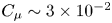 $C_{\mu } \sim 3\times 10^{-2}$ around the saturation in base pressure recovery for both forcing frequencies. The tracking highlights the formation of a train of vortices at high frequency
 $f = 1050~\textrm {Hz}$, which increases the presence density of coherent structures in the vicinity of the curved surface during the whole forcing period. There is hence an important interaction between these structures and the flow near the curved surfaces, which is absent when forcing at
 $f = 350~\textrm {Hz}$, where structures are only present in the vicinity of the curved surface for a reduced amount of time (approximately a quarter of a forcing period). This confirms the strong coupling between forcing frequency and radius of curvature discussed in § 3. The convection velocity of the coherent structures can also be evaluated based on their tracking. Interestingly, when comparing similar pulsed jet velocity forcing conditions at
 $f = 1050~\textrm {Hz}$ at different Reynolds numbers
 $Re_H = 5$ and
 $7\times 10^{5}$ in figure 20
 $(b,\!c)$, the convection velocity
 $U_c$ can be seen to remain globally constant during the forcing period but with quite different values depending on
 $Re_H$ varying from
 $0.8U_0$ to
 $0.6U_0$ at increasing
 $Re_H$. As the convection velocity is globally set by the mean velocity around the structure, this informs us that coherent structures are not positioned in the same way relative to the mean separatrix of the wake depending on
 $C_{\mu }$. Indeed, as discussed from figure 13
 $(b)$, the wake gets narrower with increasing
 $C_{\mu }$ as the mean separatrix is deflected inwards by the interaction with the curved surfaces. As a consequence, the coherent structures that are formed at a constant vertical position are evolving in a different surrounding flow: a high velocity close to or exceeding
 $U_0$ for high
 $C_{\mu }$ when the flow is importantly deviated, and a lower velocity close to the shear layer velocity
 $U_0/2$ for low
 $C_{\mu }$ when the flow is less importantly deviated. This convection velocity
 $U_c$ could be used as a further refinement in the definition of the local Strouhal number introduced in relation (3.6), as it represents the actual velocity governing the interaction of the coherent structures with the flow above the curved surface.
Streamwise convection and evolution of the circulation  $\Gamma$ of the two counter-rotating coherent structures I and II identified in figure 8 when forcing at
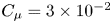 $C_{\mu } = 3\times 10^{-2}$ at
 $(a)$
 $f = 350~\textrm {Hz}$ and
 $(b)$
 $f = 1050~\textrm {Hz}$ at
 $Re_H = 5\times 10^{5}$ and at
 $(c)$
 $f = 1050~\textrm {Hz}$ at
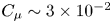 $C_{\mu } \sim 3\times 10^{-2}$ and
 $Re_H = 7\times 10^{5}$ for
 $r/h = 9$. Each marker is coloured according to the circulation
 $\Gamma$ of the coherent structure. Black lines indicate an estimation of the mean convection velocity of coherent structure I.

A.2. Formation of structure II
The formation velocity  $U_f$ in the vicinity of the slit defined and used in (4.5) to describe the formation of structure I depends on the relative position between the structure and the wake separatrix, which is highly influenced by the flow reattachment over the curved surface and the flow deviation dictated by the curved surface (similarly as discussed previously for
 $U_c$). As such, it is highly unlikely that this local flow velocity is directly the reference free-stream velocity
 $U_0$. Rather,
 $U_f$ will depend more on a combination of both
 $U_0$ fixing the velocity farther from the separating edge and the ratio
 $V_{j_{{max}}}/U_0$ dictating the flow deviation over the curved surface and the flow acceleration when circumventing the salient edge. Therefore, a pertinent, albeit gross, approximation of this complex formation process is to set the velocity
 $U_f$ involved in the formation process of structure II as a constant. To partially support this approximation, we can turn back to the convection velocity
 $U_c$ of the coherent structures analysed in figure 20, which is also a local mean flow velocity over the curved surface where the structures are transported. The convection velocity
 $U_c$ of these structures was found to vary from
 $0.8U_0$ at
 $Re_H = 5\times 10^{5}$ to
 $0.6U_0$ at
 $Re_H = 7\times 10^{5}$ for the same forcing conditions at high frequency. Nevertheless, these two convection velocities represent approximately the same dimensional velocity. The local formation velocity is set at a constant of
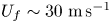 $U_f \sim 30~\textrm {m}\,\textrm {s}^{-1}$ as a gross approximation in our analysis based on a fit of the theoretical circulation
 $\Gamma _{{\text {II}}}$ to the measured circulation in figure 10
 $(b)$.
A.3. Formation of structure I
The other possible origin of structure I would be circulation produced directly by the pulsed jet similarly to the creation of II, but this hypothesis is rejected by the pulsed jet-based estimation of circulation on figure 10 $(b)$. Analogously to relation (4.5), a pulsed jet origin of the circulation contained in I would be captured by a relation
 \begin{equation} \Gamma ={-}\frac{1}{2}\int_0^{T_f} V_j(t)^{2}\,\textrm{d}t, \end{equation}
where  $T_f$ could be either the time horizon for which
 $V_j$ reaches
 $U_f$ (on similar grounds as those given for II) or
 $t_p$. Both estimations are inadequate to capture either the order of magnitude or the trend in the evolution of
 $\Gamma _{\text {I}}$ with
 $C_{\mu }$ on figure 10
 $(b)$.
Appendix B. Pressure field reconstruction validation
The method used in this study to reconstruct the mean pressure field  $\overline {C_p}$ from the PIV measurements is similar to the one used by Oxlade (Reference Oxlade2013) with adjustments on the integration algorithm to improve the efficiency of the method.
Direct integration of the mean two-dimensional momentum equations is performed where we neglect the viscous terms as we focus on a high-Reynolds-number turbulent wake flow. Hence the two-dimensional equations used for mean pressure coefficient  $\overline {C_p}$ integration are
 \begin{equation} -\frac{1}{\rho}\frac{\partial {\bar{p}}}{\partial {x}} = \overline{U_x}\frac{\partial {\overline{U_x}}}{\partial {x}} + \overline{U_z}\frac{\partial {\overline{U_z}}}{\partial {z}}+ \frac{\partial {\overline{u_x'u_x'}}}{\partial {x}} + \frac{\partial {\overline{u_x'u_z'}}}{\partial {z}} \end{equation}
and
 \begin{equation} -\frac{1}{\rho}\frac{\partial {\bar{p}}}{\partial {z}} = \overline{U_x}\frac{\partial {\overline{U_z}}}{\partial {x}} + \overline{U_z}\frac{\partial {\overline{U_z}}}{\partial {z}} + \frac{\partial {\overline{u_x'u_z'}}}{\partial {x}} + \frac{\partial {\overline{u_z'u_z'}}}{\partial {z}}. \end{equation}
The direct integration procedure is described as follows:
(i) A point
$N_k = (i,j)$ is randomly chosen in the domain and a random integration path $m_k$ is generated from this origin. Every point in the domain is given an order corresponding to its place in the path. The pressure coefficient is initialized at the origin of the path $\overline {C_p}(m_k^{0}) = \langle \overline {C_p}(m_k^{0}) \rangle _{k-1}$ by the mean pressure estimated over the first $k-1$ integration paths.(ii) The pressure is integrated to the next point in the path
$m_k^{n+1}$ according to the order given by the previously generated path and using a trapezoidal rule:
(B 3)\begin{align} \overline{C_p}(m_k^{n+1}) &= \overline{C_p}(m_k^{n}) + \frac{{\rm \Delta} x}{2}\left(\frac{\partial {\overline{C_p}}}{\partial {x}}(m_k^{n+1})+\frac{\partial {\overline{C_p}}}{\partial {x}}(m_k^{n})\right)\nonumber\\ & \quad + \frac{{\rm \Delta} y}{2}\left(\frac{\partial {\overline{C_p}}}{\partial {y}}(m_k^{n+1}) +\frac{\partial {\overline{C_p}}}{\partial {y}}(m_k^{n})\right). \end{align}(iii) The following point in the path is taken and steps 2 and 3 are repeated until all the domain is solved.
(iv) Step 1 and the rest of the procedure is repeated with a different origin and different path until statistical convergence is reached for the estimation of
$\overline {C_p}$.





The convergence criterion used is based on the residual average pressure in the domain and approximately 1500 iterations are necessary to reach satisfactory convergence.
Finally, the integration constant  $C$ is determined from using as a boundary condition Bernoulli's law on a streamline located in the potential flow region outside the wake where hypotheses linked to Bernoulli's law are satisfied:
 \begin{equation} C = (\overline{\boldsymbol{u}}_{{BC}}^{2} -1 ) + \overline{C_p}_{{BC}} \end{equation}
Examples of systematic comparison between pressure measurements on the base and reconstructed pressure field are presented in figure 21 for both unforced and forced conditions. The relative difference between the reconstructed pressure fields and the pressure measurements is  ${<}2\,\%$ (respectively,
 $5\,\%$) at maximum at a single location for taps on the curved surface. The higher discrepancy over the curved surface is attributed to the difficulty of completely properly resolving the flow with PIV near the surface due to residual laser light reflections and to the absence of seeding in the pulsed jets.
Validation of the mean pressure field  $\overline {C_p}$ reconstruction over the small FOV under different forcing conditions.
 $(a)$ Streamwise evolution on the line
 $z/H = 1.06$. Circles are pressure measurements at the base, lines the reconstructed pressure field.
 $(b)$ Comparison of pressure measurements (grey circles) and reconstructed pressure (light violet circles) over the curved surface
 $r/h = 9$.