1 Introduction
Instabilities and flow characteristics in the wake of a circular cylinder have been classical topics in fluid mechanics owing to their fundamental and practical significance. It is commonly known (e.g. Vorobieff, Georgiev & Ingber Reference Vorobieff, Georgiev and Ingber2002, Kumar & Mittal Reference Kumar and Mittal2012) that the primary (Kármán) vortex street in the near wake would transition into a two-layered vortex street in the intermediate wake (referred to as the first transition hereafter), followed by a transition from the two-layered vortices to a secondary vortex street in the far wake (referred to as the second transition hereafter). The wake transition to the secondary vortex street was first reported in an early experimental study by Taneda (Reference Taneda1959), who found that the secondary vortices had a larger spatial scale than the primary ones.
The physical mechanism for the first transition was investigated by Durgin & Karlsson (Reference Durgin and Karlsson1971), Karasudani & Funakoshi (Reference Karasudani and Funakoshi1994) and Dynnikova, Dynnikov & Guvernyuk (Reference Dynnikova, Dynnikov and Guvernyuk2016). Durgin & Karlsson (Reference Durgin and Karlsson1971) and Karasudani & Funakoshi (Reference Karasudani and Funakoshi1994) suggested that the breakdown of the primary vortex street was a result of the convection of vorticity within a vortex by the other vortices of the street. Dynnikova et al. (Reference Dynnikova, Dynnikov and Guvernyuk2016) found that the breakdown region coincides with the region of extreme dipole moment density that arises from the instability of the vortex street to the varicose disturbance of the street, including local varicose disturbance. The local varicose disturbance expands and turns into a dipole cluster that destroys the primary vortex street.
The physical mechanism for the second transition was attributed to the hydrodynamic instability of the mean wake flow in Cimbala, Nagib & Roshko (Reference Cimbala, Nagib and Roshko1988) and Williamson & Prasad (Reference Williamson and Prasad1993), and further characterised as the convective instability of the mean wake flow in Kumar & Mittal (Reference Kumar and Mittal2012). It is worth noting that these conclusions were primarily drawn from investigations of the flow at moderate Reynolds numbers (
 $Re$
) of approximately 150, where
 $Re~(=UD/\unicode[STIX]{x1D708})$
is defined based on the free-stream velocity
 $U$
, the cylinder diameter
 $D$
and the kinematic viscosity
 $\unicode[STIX]{x1D708}$
. At
 $Re=150$
, Cimbala et al. (Reference Cimbala, Nagib and Roshko1988) observed experimentally that the secondary vortex street developed well beyond 100
 $D$
downstream of the cylinder, where the frequency signal of the primary vortex street almost disappeared. As such, the secondary vortex street was not developed from amalgamation of the primary vortices. Similar results were observed in Kumar & Mittal (Reference Kumar and Mittal2012) through direct numerical simulations (DNS) at
 $Re=150$
, where the secondary vortex street was not observed in the fully developed flow up to a wake domain length of 300
 $D$
, while the frequency signal of the primary vortex street decayed to extremely small values at approximately
 $185D$
downstream of the cylinder. In contrast, an experimental study by Matsui & Okude (Reference Matsui, Okude, Dumas and Fulachier1983) at
 $Re<160$
found that the secondary vortex street was formed due to the merging of the primary vortices. Cimbala et al. (Reference Cimbala, Nagib and Roshko1988) suspected that the merging behaviour observed in Matsui & Okude (Reference Matsui, Okude, Dumas and Fulachier1983) may be due to residual smoke patterns that contained information integrated all the way back to its point of release upstream of the cylinder.
The experimental results by Williamson & Prasad (Reference Williamson and Prasad1993) at
 $Re<170$
showed that the far-wake flow was extremely sensitive to free-stream disturbances. A very small spectral peak in the free stream would lead to obvious spectral peaks at (i) the free-stream forcing frequency and (ii) the difference between the primary vortex shedding frequency and the free-stream forcing frequency. In the absence of free-stream spectral peaks, the far wake would not resonate at a specific frequency, but would exhibit a broad frequency response, and no clear structure was observed in the far wake. The effect of free-stream forcing on the far-wake flow as reported in Williamson & Prasad (Reference Williamson and Prasad1993) was confirmed numerically by Kumar & Mittal (Reference Kumar and Mittal2012) at
 $Re=150$
. The free-stream forcing effect was observed in Kumar & Mittal (Reference Kumar and Mittal2012) when the artificial excitation amplitude imposed at the free stream increased from
 $1\times 10^{-6}\,U$
to
 $2\times 10^{-5}\,U$
.
The streamwise location for the second transition has been examined by Inoue & Yamazaki (Reference Inoue and Yamazaki1999) and Vorobieff et al. (Reference Vorobieff, Georgiev and Ingber2002) through two-dimensional numerical and soap-film experimental studies for
 $Re$
up to 1000. Inoue & Yamazaki (Reference Inoue and Yamazaki1999) and Vorobieff et al. (Reference Vorobieff, Georgiev and Ingber2002) showed that the streamwise location for the second transition moved upstream with increasing
 $Re$
. Vorobieff et al. (Reference Vorobieff, Georgiev and Ingber2002) suggested that the transition location was proportional to
 $Re^{-1/2}$
.
It is noted that in most of the studies the streamwise locations for the two transitions were determined through visualisation of the instantaneous flow or vorticity field (e.g. Karasudani & Funakoshi Reference Karasudani and Funakoshi1994; Inoue & Yamazaki Reference Inoue and Yamazaki1999; Vorobieff et al. Reference Vorobieff, Georgiev and Ingber2002). Vorobieff et al. (Reference Vorobieff, Georgiev and Ingber2002) also suggested that the location for the second transition was approximately revealed by a local maximum in the relationship between the local maxima of vorticity (i.e. vorticity at vortex centres) and the streamwise distance. However, since the location for the second transition may move back and forth in time (Kumar & Mittal Reference Kumar and Mittal2012) and the vortex centres may appear at different streamwise locations for different phases, the location identified from an arbitrary vorticity field may not represent the entire time period of the flow. Hence a new method for the determination of the two transition locations is proposed in the present study (which is based on the time-averaged transverse velocity field).
In addition, the present study will investigate the intermediate- and far-wake flows of a circular cylinder for
 $Re=150$
–1000, in an attempt to complement the flow characteristics and physical mechanisms reported in the literature that focused mainly at
 $Re\sim 150$
(for which the secondary vortex street may not even appear in the domain; e.g. Kumar & Mittal Reference Kumar and Mittal2012). For
 $Re\sim 150$
, Cimbala et al. (Reference Cimbala, Nagib and Roshko1988), Williamson & Prasad (Reference Williamson and Prasad1993) and Kumar & Mittal (Reference Kumar and Mittal2012) found that the second transition in the wake of a circular cylinder was due to hydrodynamic instability of the mean flow rather than vortex merging. The second transition happened well beyond
 $100D$
downstream of the cylinder, where the frequency signal of the primary vortices was extremely weak (Cimbala et al.
Reference Cimbala, Nagib and Roshko1988; Kumar & Mittal Reference Kumar and Mittal2012). In contrast, Thompson et al. (Reference Thompson, Radi, Rao, Sheridan and Hourigan2014) found that at
 $Re=150$
the secondary vortices in the wake of an elliptical cylinder (with an aspect ratio of 0.25) were formed from merging of the two-layered vortices. The merging process happened at approximately
 $20D$
downstream of the cylinder, where individual two-layered vortices still existed. Since the second transition in the wake of a circular cylinder moves closer to the cylinder with increasing
 $Re$
(Inoue & Yamazaki Reference Inoue and Yamazaki1999; Vorobieff et al.
Reference Vorobieff, Georgiev and Ingber2002), it is speculated that the physical mechanism for the second transition may change from hydrodynamic instability of the mean flow to vortex merging (at streamwise locations where individual two-layered vortices still exist). Whether there are one or two mechanisms for the second transition of a circular cylinder warrants a further investigation. It will be shown in this study that for
 $Re=200$
–1000 the second transition in the wake of a circular cylinder is indeed due to vortex merging.
Although naturally the flow in the wake of a circular cylinder would transition to three-dimensional states for
 $Re\gtrsim 200$
(Williamson Reference Williamson1996), two-dimensional DNS in this study is justified on the following basis:
(i) Two-dimensional DNS can be used to produce laminar wake flows up to at least
 $Re=1000$
(Jiang & Cheng Reference Jiang and Cheng2017). By eliminating turbulence, the flow characteristics, variation trends and physical mechanisms identified over
$Re=200$
–1000 help to better understand the laminar flows at
$Re\sim 200$
. For example, as the vortex merging process becomes increasingly regular with time with increasing
$Re$
, the flow characteristics can be analysed more quantitatively at higher
$Re$
values and the physical mechanisms can be better understood.
(ii) The general conclusions drawn from the laminar flow results of a circular cylinder at higher
$Re$
values, including the flow characteristics, physical mechanisms and variation trends with
$Re$
, are applicable to some other laminar bluff-body flows at moderate
$Re$
values below the onset of three-dimensionality, where vortex merging is observed for the second transition at streamwise locations
${\lesssim}50D$
downstream of the cylinder (similar to the circular cylinder case at higher
$Re$
values but much smaller than the circular cylinder case at moderate
$Re$
values of 150 and 200), such as an elliptical cylinder (Thompson et al.
Reference Thompson, Radi, Rao, Sheridan and Hourigan2014), a rectangular cylinder, a flat plate and some multi-cylinder arrangements (e.g. two circular cylinders in tandem reported by Wang et al. (Reference Wang, Tian, Jia, Lu and Yin2010)). For example, it will be shown in this study that vortex merging would result in flow irregularity and frequencies other than the primary vortex shedding frequency in the two-layered and secondary vortex streets, which also holds for other bluff-body flows mentioned above.


The remainder of this paper is organised in the following manner. The governing equations and the numerical model are presented in § 2. Two typical cases at
 $Re=600$
and 300 are examined in §§ 3 and 4, respectively, followed by a summary of the variation trends with
 $Re$
in § 5. Major conclusions are drawn in § 6.
2 Numerical model
2.1 Numerical method
DNS have been carried out in this study. The governing equations are the continuity and incompressible Navier–Stokes equations:
 $$\begin{eqnarray}\displaystyle & \displaystyle \frac{\unicode[STIX]{x2202}u_{i}}{\unicode[STIX]{x2202}x_{i}}=0, & \displaystyle\end{eqnarray}$$
 $$\begin{eqnarray}\displaystyle & \displaystyle \frac{\unicode[STIX]{x2202}u_{i}}{\unicode[STIX]{x2202}t}+u_{j}\frac{\unicode[STIX]{x2202}u_{i}}{\unicode[STIX]{x2202}x_{j}}=-\frac{1}{\unicode[STIX]{x1D70C}}\frac{\unicode[STIX]{x2202}p}{\unicode[STIX]{x2202}x_{i}}+v\frac{\unicode[STIX]{x2202}^{2}u_{i}}{\unicode[STIX]{x2202}x_{j}\unicode[STIX]{x2202}x_{j}}, & \displaystyle\end{eqnarray}$$
where
 $(x_{1},x_{2})=(x,y)$
are Cartesian coordinates,
 $u_{i}$
is the velocity component in the direction
 $x_{i}$
,
 $t$
is time,
 $\unicode[STIX]{x1D70C}$
is fluid density,
 $p$
is pressure and
 $\unicode[STIX]{x1D708}$
is kinematic viscosity. The DNS are carried out with the spectral/hp element method by using an open-source code
 $\text{Nektar}++$
(Cantwell Reference Cantwell2015). The embedded unsteady Navier–Stokes solver is selected, together with a second-order implicit–explicit (IMEX) time-integration scheme, a velocity correction scheme and a continuous Galerkin projection. Hereafter, the streamwise and transverse velocities are respectively denoted as
 $u_{x}$
and
 $u_{y}$
, which are normalised with the free-stream velocity
 $U$
already.
2.2 Computational domain and mesh
The numerical simulations adopt a rectangular computational domain with the centre of the cylinder located at
 $(x,y)=(0,0)$
. The computational domain size is
 $-60\leqslant x/D\leqslant 420$
in the streamwise direction and
 $-60\leqslant y/D\leqslant 60$
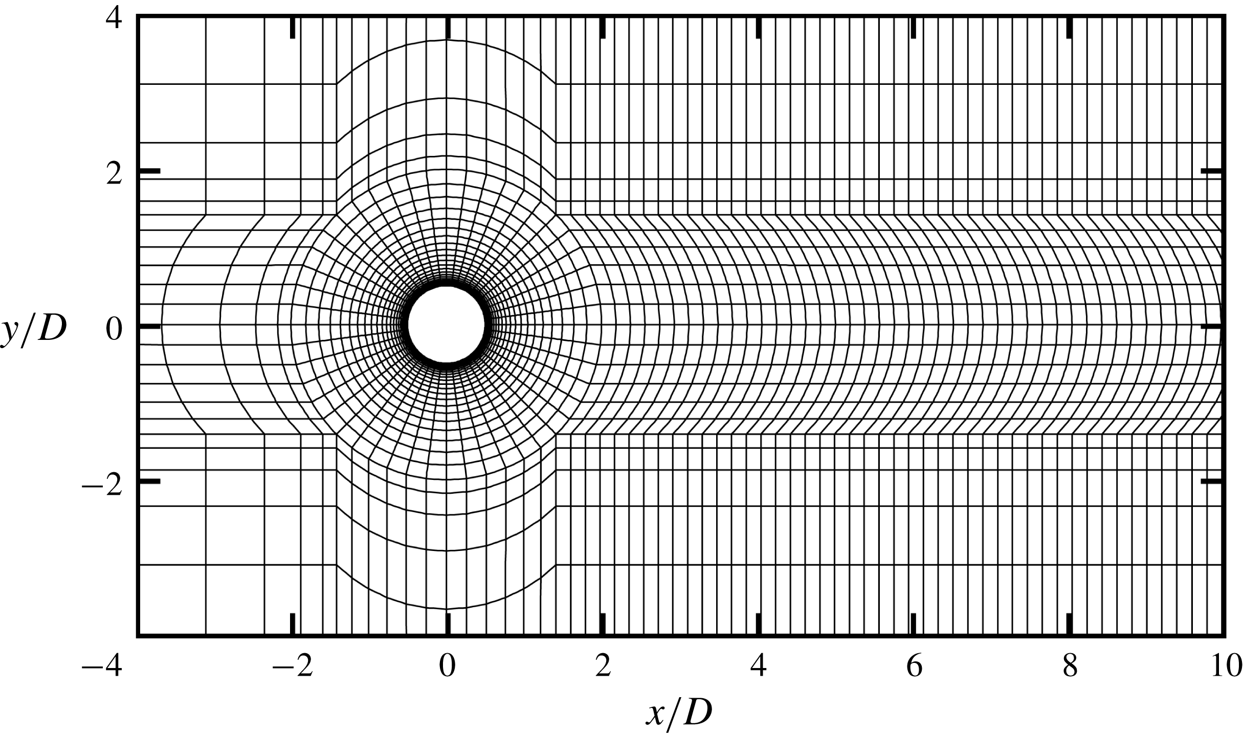
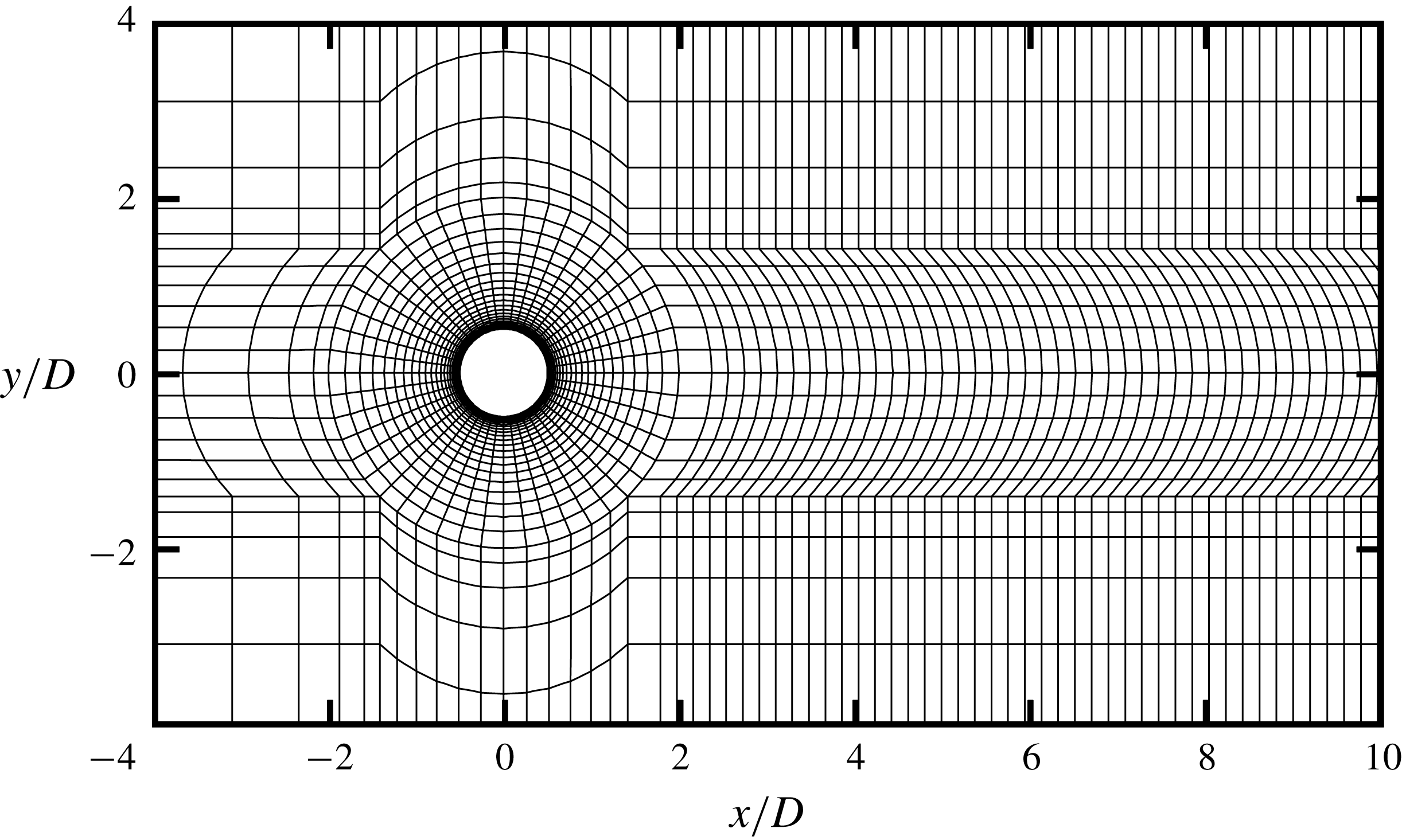
in the transverse direction. Figure 1 shows the macro-elements of the computational mesh near the cylinder. The macro-elements are further subdivided using fifth-order Lagrange polynomials (
 $N_{p}=5$
) on the Gauss–Lobatto–Legendre points for the quadrilateral expansions. In figure 1, the cylinder perimeter is discretised with 48 macro-elements, and the radial size of the first layer of macro-elements next to the cylinder is
 $0.0055D$
. To capture detailed near-wake and far-wake flow structures, a relatively high mesh resolution is used in the wake region by specifying the streamwise size of the macro-elements at the wake centreline (
 $y=0$
) varying linearly from
 $0.1875D$
at
 $x/D=2$
to
 $2.5\times 0.1875D$
at
 $x/D=400$
. The computational mesh consists of a total of 46 091 macro-elements, of which approximately 44 000 macro-elements are placed in the region of
 $x/D>2$
because the transition to the secondary vortex street (especially at low
 $Re$
values such as
 $Re=200$
) is extremely disturbance-dependent (Thompson et al.
Reference Thompson, Radi, Rao, Sheridan and Hourigan2014) and therefore mesh-dependent. A detailed mesh independence check is reported in Appendix A.
Macro-elements of the computational mesh near the cylinder.

The boundary conditions are specified as follows. At the inlet and transverse sides, a uniform velocity (
 $U$
, 0) is specified. At the outlet, the Neumann boundary condition (i.e. a zero normal gradient) is applied for the velocity. At the cylinder surface, the no-slip condition is imposed for the velocity. The pressure at the outlet is specified as a reference value of zero, while the pressure at all other boundaries uses a high-order Neumann boundary condition.
The internal flow follows an impulsive start at the beginning of the simulation. The time step size is chosen based on the criterion that the Courant–Friedrichs–Lewy (CFL) number is kept below 0.5.
With a focus on the near-wake primary vortex street, Henderson (Reference Henderson1997) found that the two-dimensional flow in the wake of a circular cylinder is perfectly time-periodic for
 $Re$
up to at least 1000. However, as will be shown in § 3.4, the flow starts to become slightly aperiodic when the primary vortex street is about to break down to form the two-layered vortices. In the present study, each case is first calculated for at least 1800 non-dimensional time units (defined as
 $t^{\ast }=tU/D$
) to ensure that the entire wake flow has become fully developed. Since the intermediate- and far-wake flows are aperiodic, each case is run for at least another 900 non-dimensional time units (i.e. at least 200 primary vortex shedding cycles) to achieve meaningful results that are statistically stationary.
3 Results at
$Re=600$

The flow characteristics in the wake of a circular cylinder are examined for
 $Re=150$
–1000. Apart from the case of
 $Re=150$
where the secondary vortex street is not observed within
 $x/D\leqslant 400$
, two different development processes of the secondary vortices are observed for
 $Re=200$
–300 and 400–1000, which are illustrated with two typical cases
 $Re=300$
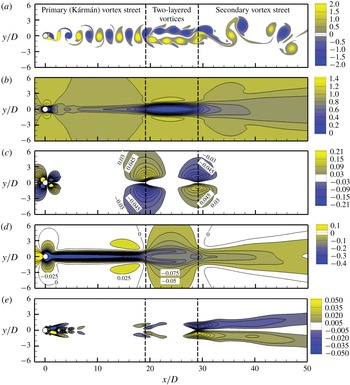
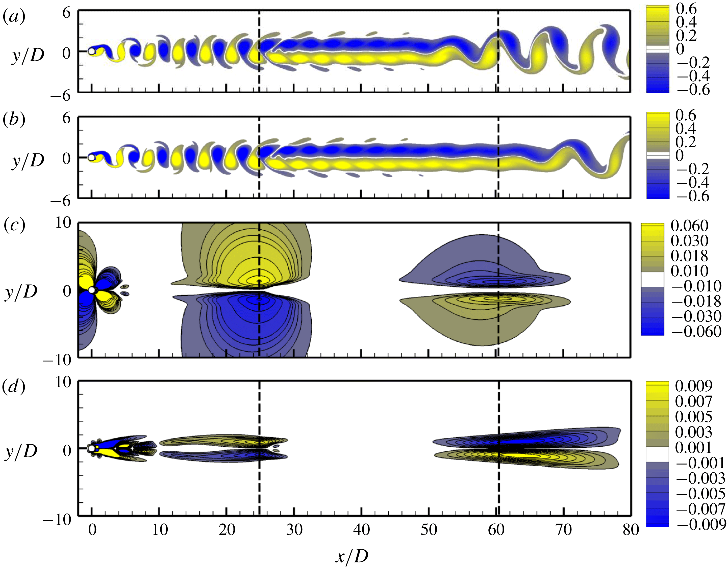
and 600 in §§ 4 and 3, respectively. Figure 2(a) shows the instantaneous vorticity field for
 $Re=600$
at a non-dimensional time instant
 $t^{\ast }=2800$
, where the entire wake flow is fully developed. The wake flow can be separated into three regimes, namely the primary (Kármán) vortex street, the two-layered vortices and the secondary vortex street.
Flow characteristics for
 $Re=600$
: (a) instantaneous vorticity field at
 $t^{\ast }=2800$
, (b) time-averaged streamwise velocity field, (c) time-averaged transverse velocity field, (d) time-averaged pressure field, and (e) time-averaged Reynolds stress field. The two transition locations are marked by the vertical dashed lines.

3.1 Time-averaged flow
Figure 2(b–e) shows some flow characteristics for
 $Re=600$
that are averaged over 950 non-dimensional time units. The time-averaged contours are generally symmetric about the wake centreline, which suggests that the statistical range is sufficient. Very slight asymmetries about the wake centreline are observed in figure 2(b,d,e) at
 $x/D\gtrsim 38$
, which is because the secondary vortex street in the far wake is highly spatially irregular (figure 2
a) and therefore a perfectly symmetric time-averaged flow would require a significant amount of statistical time period. Since the exact symmetry of the secondary vortex street is not the main focus of the study, a further increase in the statistical range is not attempted. Dynnikova et al. (Reference Dynnikova, Dynnikov and Guvernyuk2016) also presented similar patterns of the time-averaged velocity fields for
 $Re=600$
.
In the present study, the streamwise locations for the first and second transitions are determined by the time-averaged
 $u_{y}$
field shown in figure 2(c). Two pairs of local maxima are observed in figure 2(c) at
 $x/D=19.1$
and 29.1 (as marked by two vertical dashed lines). The positive and negative maxima in each pair are symmetric about the wake centreline. The first location
 $x/D=19.1$
corresponds to the first transition (see figure 2
a), where the flow is diverted away from the wake centreline. Hence a positive maximum in the
 $u_{y}$
field is observed above the wake centreline while a negative maximum is observed below the wake centreline (figure 2
c). The second location
 $x/D=29.1$
corresponds to the second transition (see figure 2
a), where the flow starts to reoccupy the wake centreline. Hence a negative maximum in the
 $u_{y}$
field is observed above the wake centreline while a positive maximum is observed below the wake centreline (figure 2
c). The local maxima in the
 $u_{y}$
field are the locations where the flow diversions are most pronounced, and therefore these locations are defined as the transition locations.
The transition locations are marked in all the time-averaged flow fields shown in figure 2. Distinct features at the transition locations are observed in each of the panels. For the time-averaged Reynolds stress
 $(u_{x}^{\prime }u_{y}^{\prime })$
field shown in figure 2(e), local maxima also appear at the transition locations, where the flow shearing is the strongest. The
 $u_{x}^{\prime }$
and
 $u_{y}^{\prime }$
values are defined as
 $$\begin{eqnarray}\displaystyle & \displaystyle u_{x}^{\prime }=\sqrt{\frac{1}{N}\mathop{\sum }_{i=1}^{N}(u_{x,i}-\bar{u}_{x})^{2}}, & \displaystyle\end{eqnarray}$$
 $$\begin{eqnarray}\displaystyle & \displaystyle u_{y}^{\prime }=\sqrt{\frac{1}{N}\mathop{\sum }_{i=1}^{N}(u_{y,i}-\bar{u}_{y})^{2}}, & \displaystyle\end{eqnarray}$$
where
 $N$
is the number of values in the time history, and the overbar denotes the time-averaged value. For the time-averaged
 $u_{x}$
field shown in figure 2(b), large gradients in
 $u_{x}$
are observed at the wake centreline at approximately the two transition locations, which is due to the flow diversion in the transverse direction. Between the two transition locations (where the two-layered vortices take place), the streamwise velocity near the wake centreline decreases to extremely small values, as indicated by the blue area in figure 2(b). This area was called the ‘calm region’ in Durgin & Karlsson (Reference Durgin and Karlsson1971). The flow and vortices largely travel around this calm region rather than through it. Consistently, a rapid recovery (reduction) of the negative pressure at the location of the first transition is observed in figure 2(d).
3.2 Frequencies in the wake
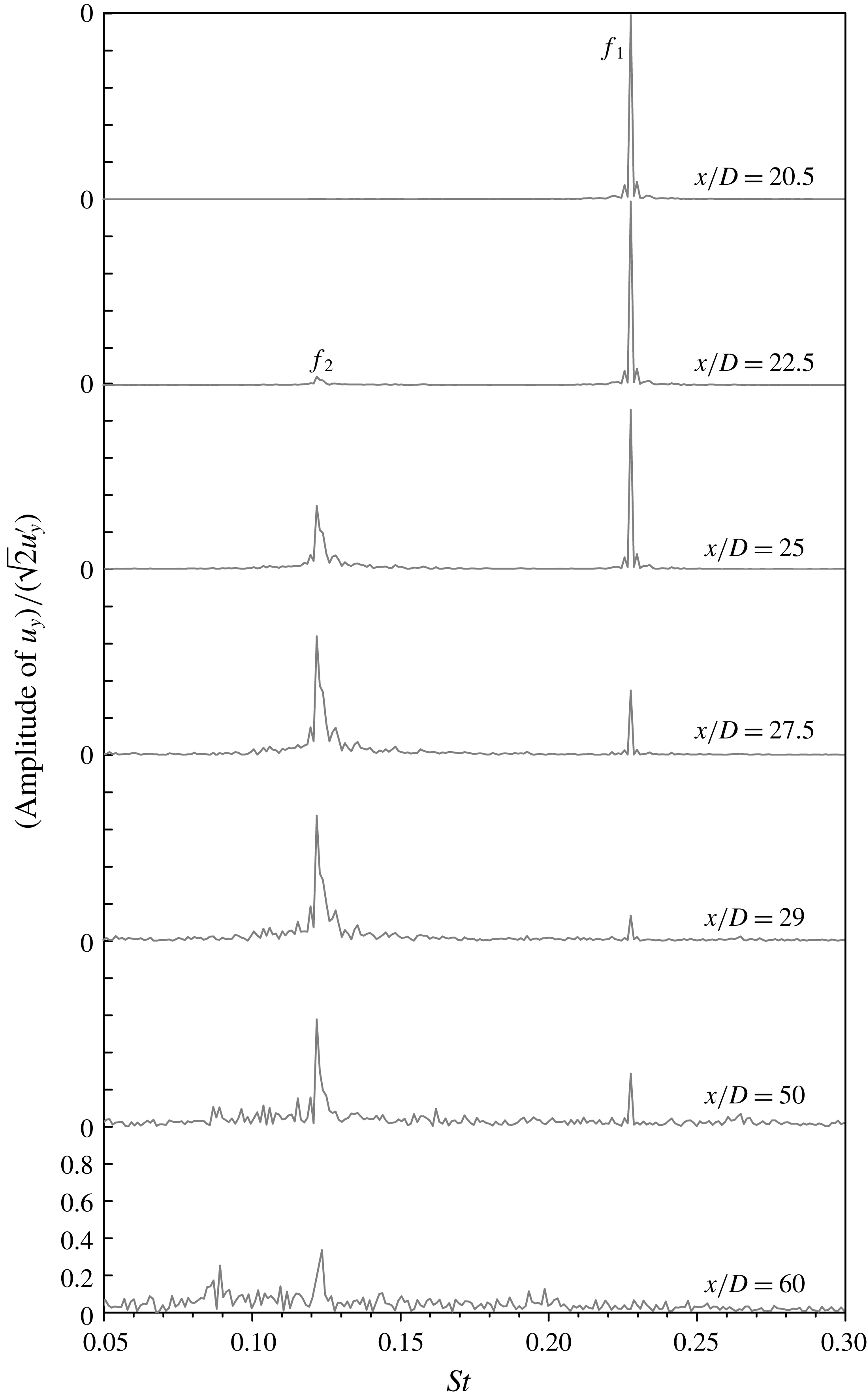
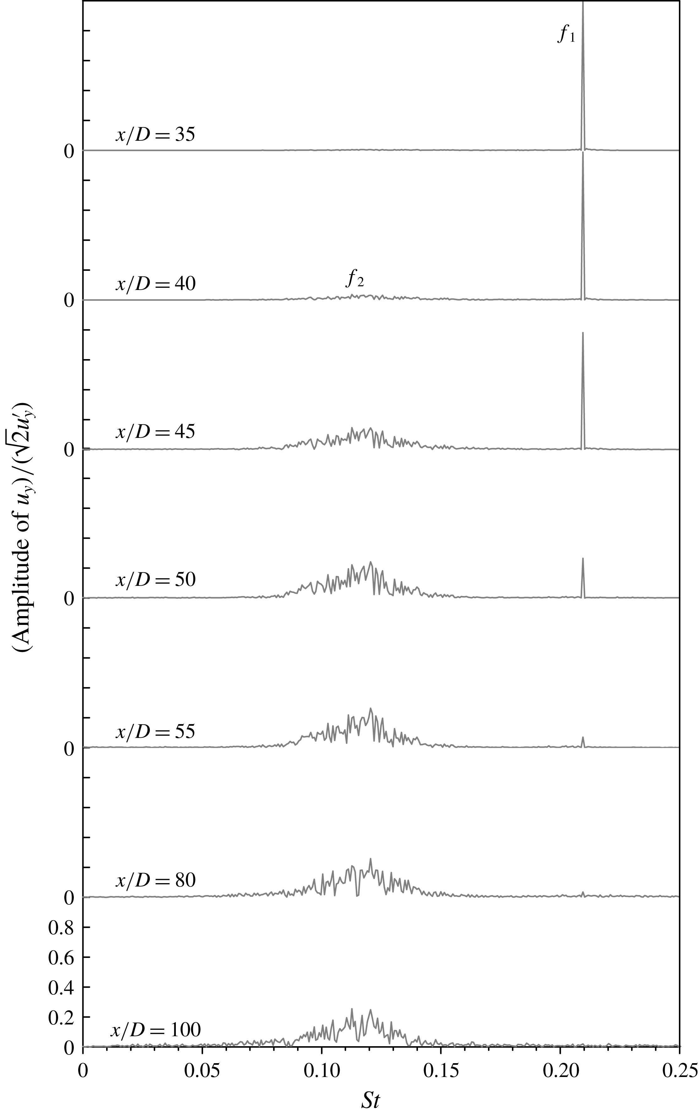
Figure 3 shows the frequency spectra of the time histories of
 $u_{y}$
sampled at
 $y=0$
and various streamwise locations. The frequency spectra are calculated from the fast Fourier transform (FFT) of the time history of
 $u_{y}$
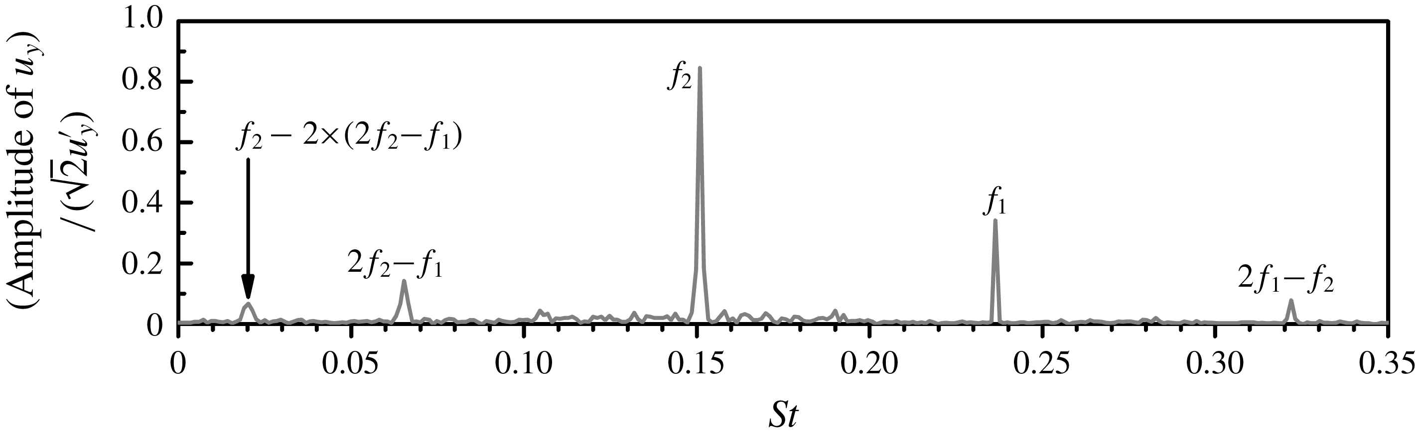
over a period of 215 primary vortex shedding periods. Two sharp peaks
 $f_{1}$
and
 $f_{2}$
are observed in the frequency spectra shown in figure 3. The first peak
 $f_{1}$
, which contains only a single frequency value, represents the primary vortex shedding frequency. The second peak
 $f_{2}$
, which consists of a sharp peak together with small-scale broad-band frequencies at the two sides of the peak, is associated with the development of the secondary vortex street.
Frequency spectra of
 $u_{y}$
for
 $Re=600$
. The time histories of
 $u_{y}$
are sampled at
 $y=0$
and various streamwise locations. The frequency spectra are calculated from the FFT of the time history of
 $u_{y}$
over a period of 215 primary vortex shedding cycles.

In figure 3, the amplitude of
 $u_{y}$
is normalised by
 $1/(\sqrt{2}u_{y}^{\prime })$
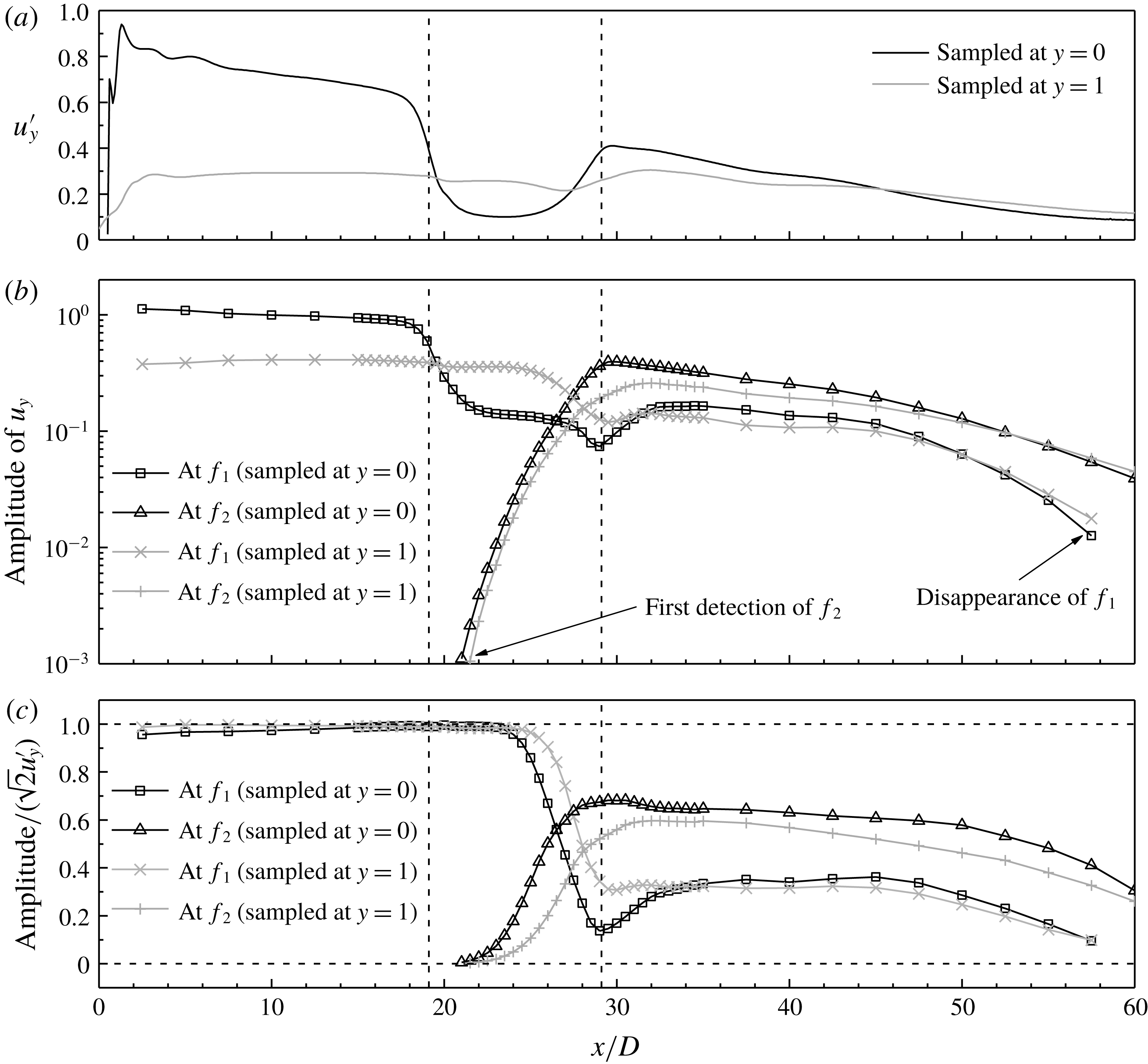
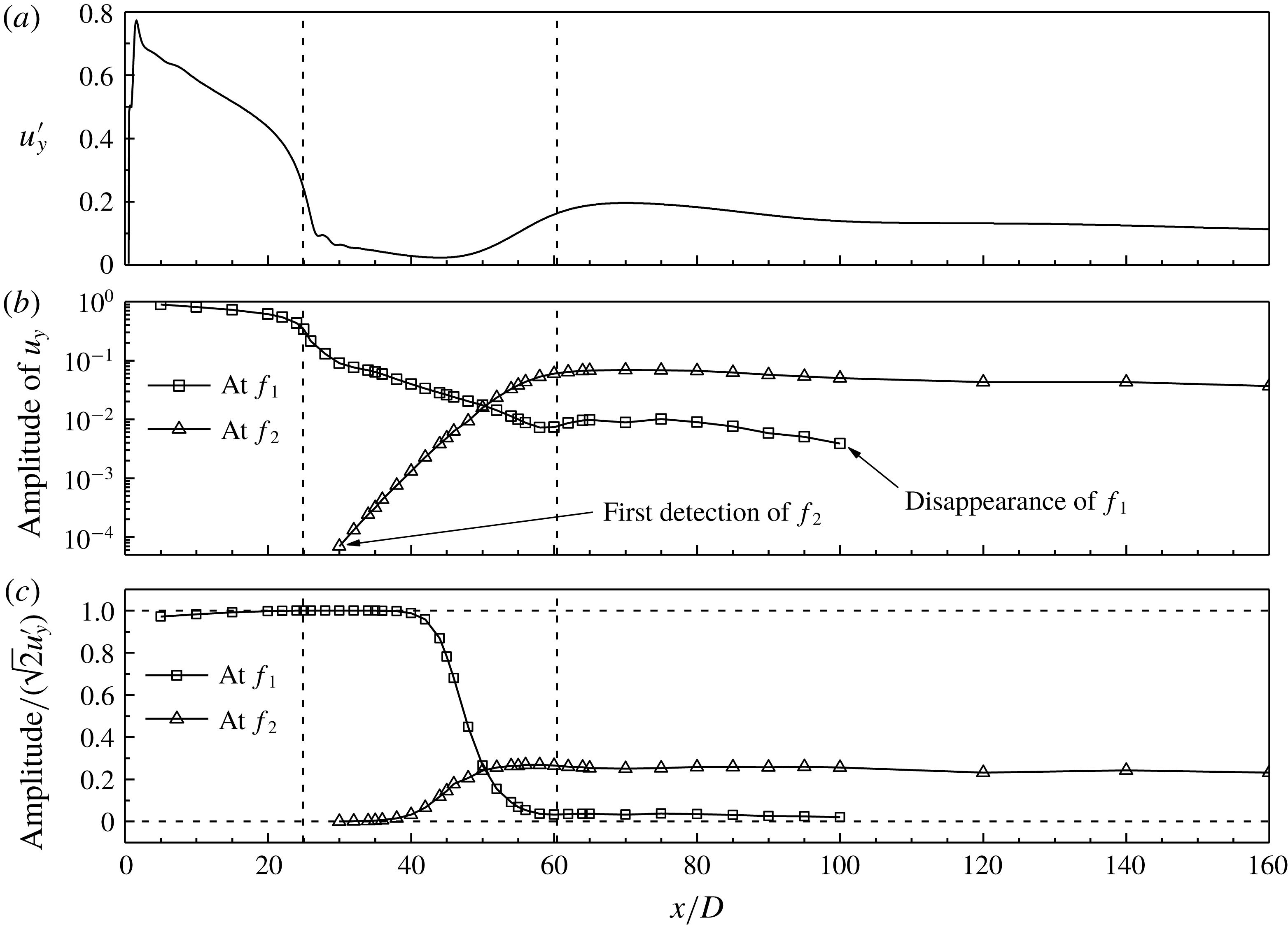
. Figure 4(c) shows the normalised peak amplitude of
 $u_{y}$
at each of the two frequencies
 $f_{1}$
and
 $f_{2}$
as a function of the streamwise location. The reason for the normalisation is explained with the results before normalisation in figure 4(b). The amplitude of
 $u_{y}$
shown in figure 4(b) is controlled by two aspects. One is the fluctuation amplitude of the
 $u_{y}$
signal, and the other is the relative strengths of the two frequencies. The fluctuation amplitude of the
 $u_{y}$
signal can be quantified by the
 $u_{y}^{\prime }$
value shown in figure 4(a). The
 $u_{y}^{\prime }$
curve sampled at
 $y=0$
displays an obvious trough over the calm region, while the
 $u_{y}^{\prime }$
curve sampled at
 $y=1$
(out of the calm region) is much steadier. Different features in the
 $u_{y}^{\prime }$
versus
 $x/D$
relationship (figure 4
a) would influence the amplitude of
 $u_{y}$
versus
 $x/D$
relationship shown in figure 4(b) significantly. For example, the rapid drop in the amplitude of
 $u_{y}$
at
 $f_{1}$
over
 $x/D\sim 18$
–22 (along
 $y=0$
) is completely due to a corresponding drop in the
 $u_{y}^{\prime }$
value over the same range of
 $x/D$
. To eliminate such an influence, the amplitude of
 $u_{y}$
is normalised by
 $1/(\sqrt{2}u_{y}^{\prime })$
in figure 4(c). After normalisation, the normalised amplitude becomes 1.0 if the time history of
 $u_{y}$
is perfectly sinusoidal (with an arbitrary amplitude and frequency).
Variation of the amplitude of
 $u_{y}$
with the streamwise location for
 $Re=600$
. The amplitude of
 $u_{y}$
is examined with (a) root-mean-square of
 $u_{y}$
, (b) amplitude of
 $u_{y}$
at the two frequencies
 $f_{1}$
and
 $f_{2}$
, and (c) normalised amplitude of
 $u_{y}$
at the two frequencies
 $f_{1}$
and
 $f_{2}$
. The two transition locations are marked by the vertical dashed lines.

As shown in figure 4(c), the normalised amplitude at
 $f_{1}$
(sampled at
 $y=0$
) is very close to 1.0 for the range of
 $x/D\lesssim 22$
. This is because for
 $x/D\lesssim 22$
the frequency spectra of
 $u_{y}$
are dominated by a single frequency value
 $f_{1}$
(figure 3). The small deviation from 1.0 is because the time history of
 $u_{y}$
is not perfectly sinusoidal. It is also seen in figure 4(c) that
 $f_{2}$
emerges at
 $x/D=21$
, which is slightly after the transition to the two-layered vortices. For
 $x/D$
from the first detection of
 $f_{2}$
to the onset of the secondary vortex street, there is a gradual increase in the normalised amplitude at
 $f_{2}$
. Correspondingly, there is a gradual decrease in the normalised amplitude at
 $f_{1}$
, since the fluctuation amplitude of the
 $u_{y}$
signal is increasingly contributed by
 $f_{2}$
rather than
 $f_{1}$
. After normalisation, similar variation trends are observed in figure 4(c) for the results sampled at
 $y=0$
and 1.
After the development of the secondary vortices over a short streamwise distance, the normalised amplitudes at
 $f_{1}$
and
 $f_{2}$
decay with distance downstream at
 $x/D\gtrsim 45$
. The two peaks at
 $f_{1}$
and
 $f_{2}$
would eventually disappear into the noise level. For example, figure 3 shows that
 $f_{1}$
is no longer observed at
 $x/D\sim 60$
.
3.3 Time evolution of the vortices
Figure 5 shows a typical sequence of the instantaneous vorticity fields for
 $Re=600$
(see also the supplementary movie ‘Movie1.mp4’ available online at https://doi.org/10.1017/jfm.2019.167). The vorticity fields are shown at
 $t^{\ast }=1860+nT_{1}$
, where
 $T_{1}~(=1/f_{1})$
is the primary vortex shedding period, and
 $n=1$
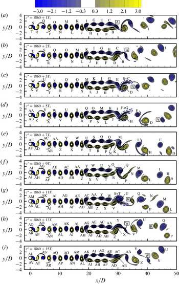
, 2, 3 and odd integers up to 15. To facilitate tracing of the time evolution of the vortices, the same vortices that appear in different snapshots are labelled with the same letters.
A sequence of the instantaneous vorticity fields at
 $Re=600$
. The vorticity contours are shown from
 $-3$
to 3 with an interval of 0.3. The same vortices that appear in different snapshots are labelled with the same letters. The single vortices are marked by a rectangular frame around the vortex letter. The time evolution of the vorticity field can also be seen from the online supplementary movie ‘Movie1.mp4’ accompanying this article.

Based on flow visualisation, it is seen in figure 5 that the vorticity fields are highly repeatable for
 $x/D<24$
. In particular, the first transition at
 $x/D=19.1$
is a highly repeatable alternate rearrangement of the positive and negative vortices into two rows of vortices with the same sign. For
 $21<x/D<24$
, although
 $f_{2}$
is detected, its amplitude is still at least approximately one order of magnitude lower than that at
 $f_{1}$
(figure 4
b), such that its influence is expected to be rather small. The flow becomes visually irregular when the normalised amplitudes at
 $f_{1}$
and
 $f_{2}$
exhibit obvious decrease (from 1.0) and increase (from 0), respectively (figure 4
c).
The vortices start to become irregular when they start to rearrange themselves for the second transition. The second transition at
 $x/D=29.1$
is an irregular pairing and merging process. A typical pairing and merging cycle, as illustrated in figure 5(b,c), takes a period of approximately
 $2T_{1}$
. It starts with the pairing of a positive vortex B and a negative vortex C in figure 5(b). The two vortices become stretched after encountering each other. Meanwhile, two vortices D and E are located at the two sides of the B
 $+$
C pair. The pairing of B
 $+$
C blocks the path for the subsequent pairing of D and E. Hence instead of pairing, D and E further squeeze the B
 $+$
C pair into a highly stretched pattern, as shown by the dashed blue line in figure 5(c). The B
 $+$
C pair is then dismembered through the following processes:
(i) With the rotation of D and E, B is partly merged into D while C is partly merged into E. The merging starts from the lower left end of the B
$+$
C pair. The positive and negative vortices may not merge simultaneously. For example, the merging of the positive vortices happens earlier in the three pairing and merging cycles shown in figure 5(c–e).(ii) During the above process, B and C may partly cancel each other.
(iii) The remaining part may form a shear layer (e.g. the shear layer between vortices D and E in figure 5 d).

Eventually, vortices B and C disappear while vortices D and E remain in the far wake.
The second and third pairing and merging cycles shown in figure 5(d,e) are similar to the first cycle shown in figure 5(b,c), while the fourth cycle in figure 5(f) is slightly different. Through examining a number of phases of the four cycles (see the online supplementary movie ‘Movie1.mp4’), it is found that with the evolution of the cycles there is a gradually enhanced spatial mismatch of the two vortices at pairing. The positive vortex becomes increasingly downstream of the negative one. For the fourth cycle, there is an obvious mismatch of the pairing of vortices N and O. Consequently, the positive vortex N is barely merged into vortex P, while the negative vortex O is largely merged into vortex Q. The majority of vortex N becomes an obvious shear layer (or even a vortex) in the far wake (figure 5 g).
The mismatch at the pairing becomes more significant in the fifth cycle shown in figure 5(g). Since vortex R is increasingly downstream of vortex S (figure 5 f), it becomes a single vortex (without being paired) at the formation of the secondary vortex street (figure 5 g). The single vortices shown in figure 5 are marked by a rectangular frame around the vortex letter. Vortex S is then paired with vortex T, and this vortex pair is subsequently merged into vortices U and V (figure 5 g).
The mismatch at the pairing that results in a single vortex would induce a subsequent mismatch that leads to another single vortex with the opposite sign. For the sixth cycle shown in figure 5(h), a negative single vortex W is observed prior to the pairing of X and Y. In addition, Y is slightly downstream of X, such that Y is barely merged into AA, while X is largely merged into Z. The majority of Y becomes an obvious vortex in the far wake (figure 5 i). It is worth noting that the formation mechanisms for vortices W and Y are different. Vortex W is a single vortex originated from the mismatch at the point of pairing and merging, while vortex Y is a remaining part after the pairing and merging of vortices X, Y, Z and AA.
For the seventh cycle shown in figure 5(i), there is no mismatch over the pairing of AB and AC. This cycle is similar to the first three cycles shown in figure 5(b–e).
The time evolution of the vortices is further visualised for a period of 501 non-dimensional time units. This time period is equal to both
 $114T_{1}$
and
 $61T_{2}$
(where
 $T_{2}=1/f_{2}$
). The starting point of the time period is the pairing of B and C in the first cycle shown in figure 5(b). In other words, the time period covers
 $t^{\ast }=1860+2T_{1}$
to
 $1860+116T_{1}$
. Over this time period, a total of 53 pairing and merging cycles are observed, together with the emergence of an extra eight positive and eight negative single vortices due to the mismatch (e.g. vortices R and W in figure 5). In total, the two-layered vortices, which contain 114 positive and 114 negative vortices, are paired and merged into 61 (
 $=53+8$
) positive and 61 negative vortices, which is identical to
 $61T_{2}$
for this time period.
In addition to flow visualisation, the time evolution of the vortices can also be quantified by the time histories of
 $u_{y}$
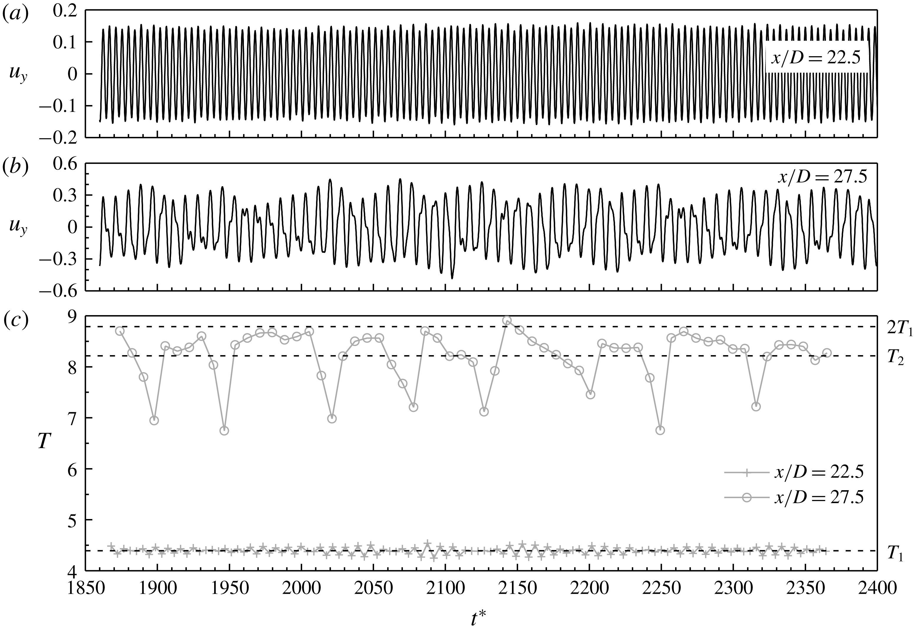
sampled in the wake. Figure 6(a,b) shows the time histories of
 $u_{y}$
sampled along
 $y=0$
at
 $x/D=22.5$
and 27.5. Figure 6(c) shows the period
 $T$
of each cycle of the time histories shown in figure 6(a,b) over a range of
 $1860+2T_{1}$
to
 $1860+116T_{1}$
. At
 $x/D=22.5$
, the two-layered vortices are stably formed (figure 5). The flow is dominated by the primary vortex shedding frequency
 $f_{1}$
, while the influence of
 $f_{2}$
is negligibly small (see figure 3). As shown in figure 6(c), there are 114 cycles for the time history of
 $u_{y}$
sampled at
 $x/D=22.5$
, and their periods are all very close to
 $T_{1}$
, such that a single frequency peak
 $f_{1}$
is observed in figure 3.
At
 $x/D=27.5$
, the two-layered vortices are about to pair and merge and no longer in a parallel pattern (figure 5). The time history of
 $u_{y}$
shown in figure 6(b) is modulated by
 $f_{2}$
significantly, and the corresponding frequency spectrum shown in figure 3 is dominated by
 $f_{2}$
rather than
 $f_{1}$
. As shown in figure 6(c), there are 61 cycles for the time history of
 $u_{y}$
sampled at
 $x/D=27.5$
, which is consistent with the visualisation of 61 positive and 61 negative vortices at the pairing and merging process. The variation of
 $T$
for the time history of
 $u_{y}$
sampled at
 $x/D=27.5$
is larger than that sampled at
 $x/D=22.5$
. Hence the frequency range of
 $f_{2}$
is wider than that of
 $f_{1}$
(figure 3). The peak frequency
 $f_{2}$
corresponds to the period
 $T_{2}$
shown in figure 6(c). It is also noted that
 $T_{2}~(=8.21)$
is very close to the averaged period of 8.19. For an ideal condition where the pairing and merging process does not generate mismatched single vortices, one would expect
 $T_{2}=2T_{1}$
(i.e.
 $2f_{2}=f_{1}$
). As shown in figure 6(c), the periods for the time history of
 $u_{y}$
sampled at
 $x/D=27.5$
are capped at approximately
 $2T_{1}$
. Owing to the frequent generation of the single vortices, the periods are reduced from
 $2T_{1}$
. In particular, eight obvious troughs are observed in the time history of
 $T$
, which is consistent with the visualisation of eight positive and eight negative single vortices. It is also noticed from the time history of
 $T$
that the single vortices are generated every few pairing and merging cycles, but this process is not exactly regular.
Time histories of
 $u_{y}$
sampled at
 $y=0$
and
 $x/D=22.5$
(a) and 27.5 (b). In addition, panel (c) shows the period
 $T$
of each cycle of the time histories over a range of
 $1860+2T_{1}$
to
 $1860+116T_{1}$
.

3.4 Irregularity of the flow
As mentioned in § 3.3, the instantaneous vorticity fields shown in figure 5 become visually irregular at
 $x/D>24$
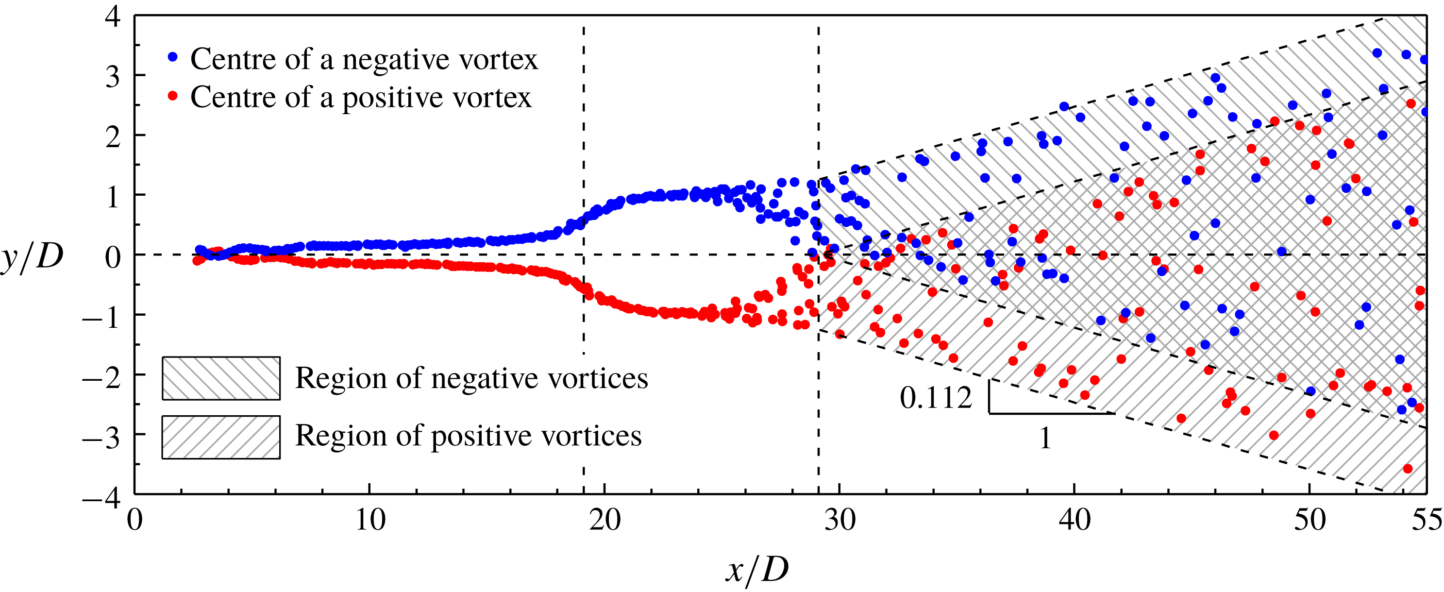
. The irregularity of the flow is further shown in figure 7 by the spatial distribution of the vortex centres. The vortex centres are extracted from 22 snapshots of the vorticity field at different phases (in contrast to figure 5 for the same phase). For
 $x/D<24$
, the centres of positive and negative vortices follow two clear trajectories on the two sides of the wake centreline. The spatial locations of the vortices start to become visually irregular at
 $x/D>24$
when they start to rearrange themselves for the irregular pairing and merging process. After the second transition at
 $x/D=29.1$
, the positive vortex centres may enter the upper half-domain, while the negative vortex centres may enter the lower half-domain. As the vortices propagate along the streamwise direction, the spatial regions of positive and negative vortices (as shaded in figure 7) both expand along the two sides of the transverse direction. The spatial expansion ratio is approximately
 $y:x=0.112$
. Within the two shaded regions for the positive and negative vortices, the spatial distribution of the vortices is irregular.
Spatial distribution of the vortex centres for
 $Re=600$
. The vertical dashed lines mark the two transition locations, while the horizontal dashed line marks the wake centreline.

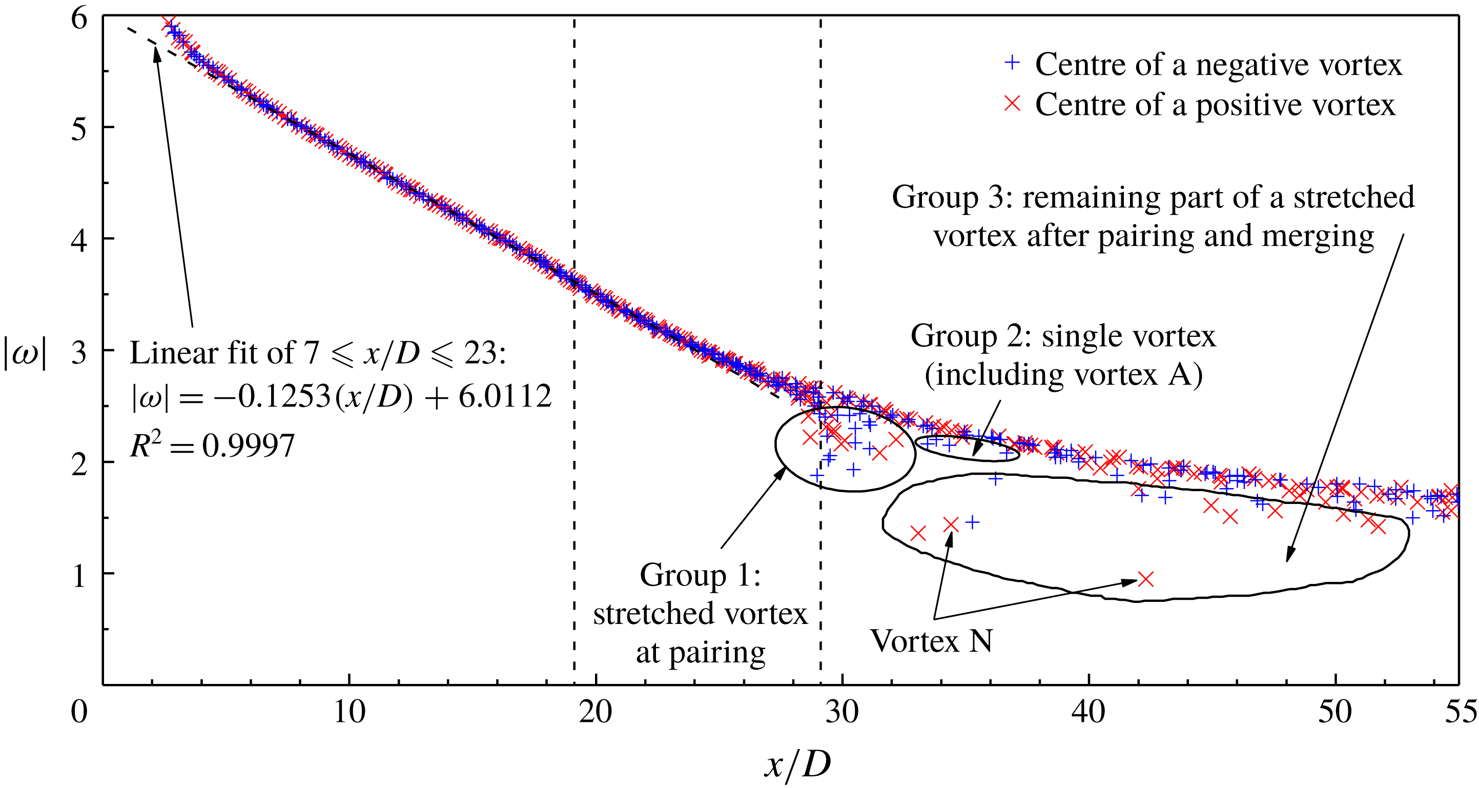
For the vortex centres identified in figure 7, the absolute value of the vorticity at the vortex centre is plotted in figure 8 as a function of the streamwise location. Within the first few cylinder diameters of the near wake, the primary vortices undergo intensive rotation after being shed from the cylinder surface, and a nonlinear drop of the vorticity with
 $x/D$
is observed in figure 8. After that, a linear decay of the vorticity is observed as the vortex propagates in the range of
 $7\leqslant x/D\leqslant 23$
. This range includes the first transition at
 $x/D=19.1$
, which is because at this transition the vortices are not subjected to splitting or merging.
Absolute value of the vorticity at the vortex centre as a function of the streamwise location for
 $Re=600$
. The two transition locations are marked by the vertical dashed lines.

However, after the second transition at
 $x/D=29.1$
, some vorticity values appear to be lower than the main curve, as circled in the three groups in figure 8. Group 1 at around
 $x/D=29.1$
is induced by the stretched vortices at pairing (e.g. vortices B and C in figure 5). The vorticity is decreased because the vortex pair may partly cancel each other over the vortex pairing process, and partly merged into subsequent vortices over the vortex merging process. Group 2 consists of the single vortices (e.g. vortex A in figure 5). The vorticity is slightly smaller because the single vortices are generated without vortex merging. Group 3 consists of the remaining parts of the stretched vortices after the pairing and merging process (e.g. vortex N in figure 5).
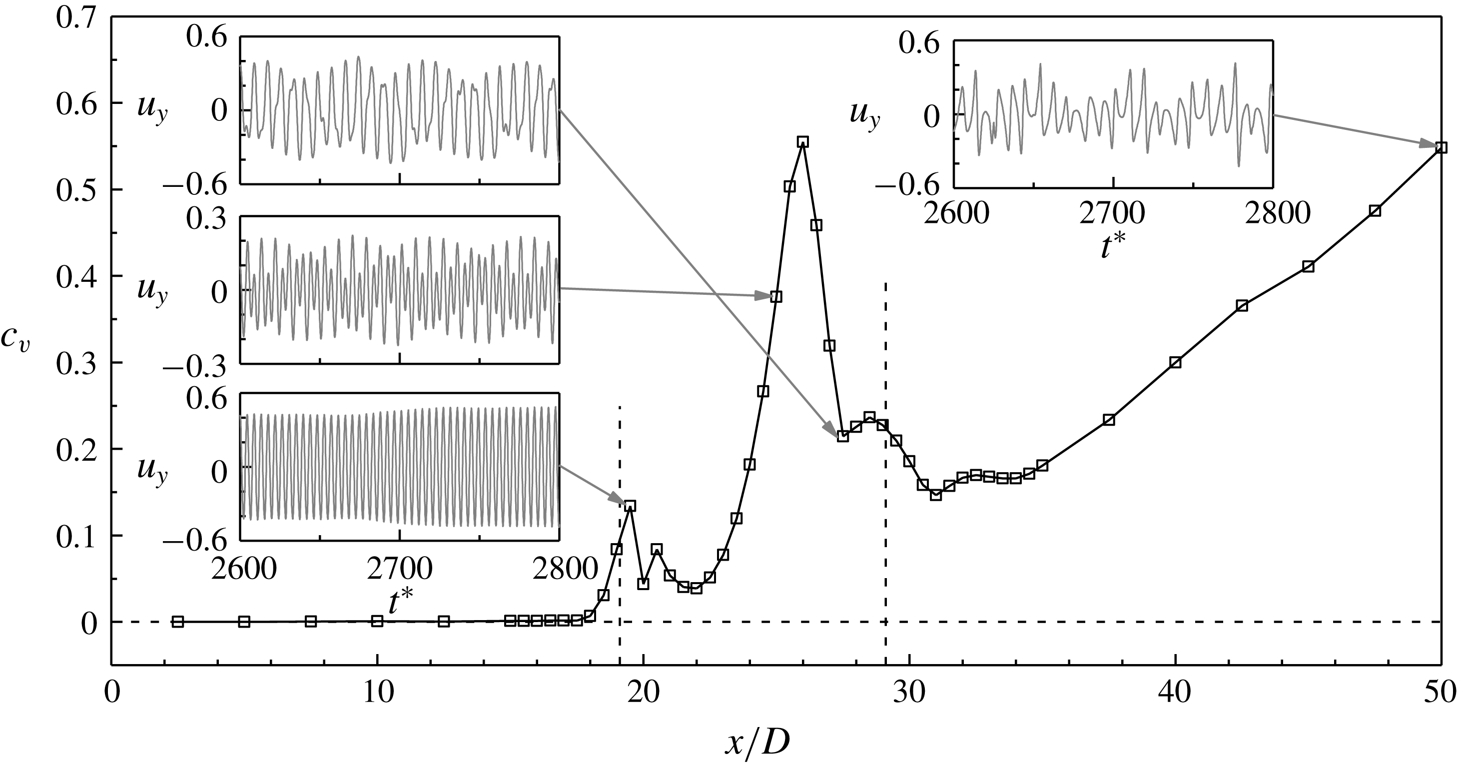
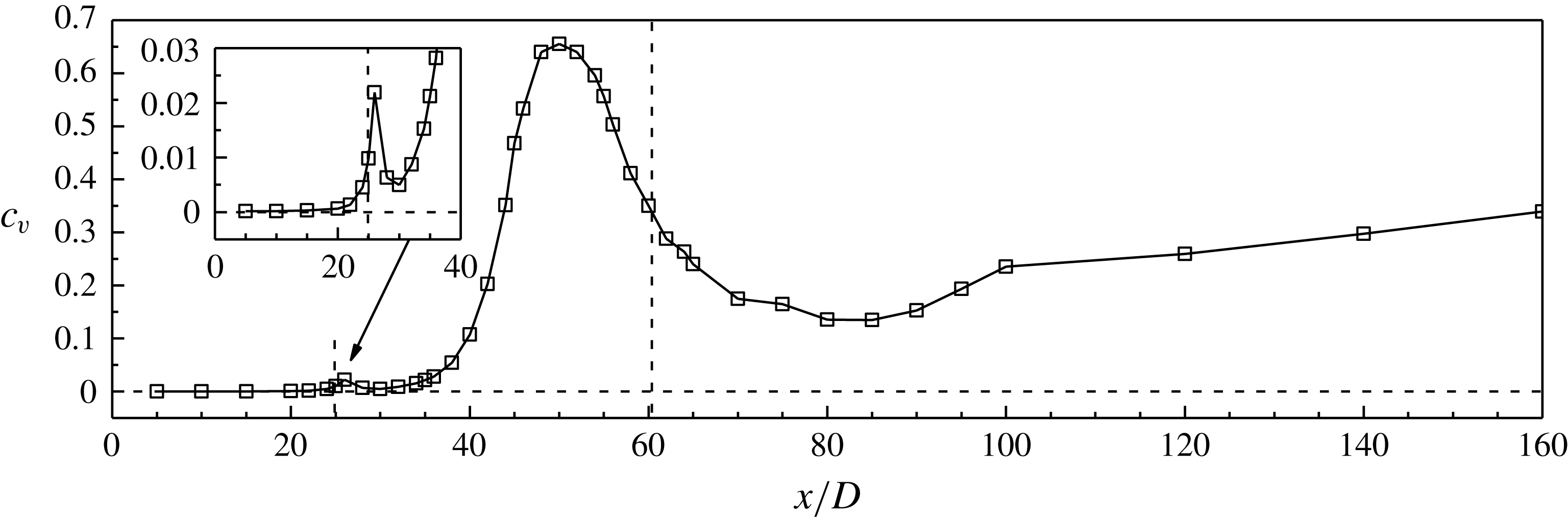
The irregularity of the wake flow is further quantified by the irregularity of the time histories of
 $u_{y}$
sampled at various streamwise locations. The irregularity of a time history can be quantified by the coefficient of variation (
 $c_{v}$
) of the positive and negative peak values extracted from each period of the time history. The positive and negative peak values form two series of data
 $a_{i}$
and
 $b_{i}$
. The coefficient of variation for the positive and negative peaks are calculated as
 $$\begin{eqnarray}\displaystyle & \displaystyle c_{v,positive}=\frac{\sqrt{\displaystyle \frac{1}{N}\mathop{\sum }_{i=1}^{N}(a_{i}-\bar{a})^{2}}}{|\bar{a}-\bar{u}_{y}|}, & \displaystyle\end{eqnarray}$$
 $$\begin{eqnarray}\displaystyle & \displaystyle c_{v,negative}=\frac{\sqrt{\displaystyle \frac{1}{N}\mathop{\sum }_{i=1}^{N}(b_{i}-\bar{b})^{2}}}{|\bar{b}-\bar{u}_{y}|}, & \displaystyle\end{eqnarray}$$
where
 $N$
is the number of values in
 $a_{i}$
and
 $b_{i}$
, and the overbar denotes the averaged value. The coefficient of variation for the time history is determined as
 $$\begin{eqnarray}c_{v}=\frac{c_{v,positive}+c_{v,negative}}{2}.\end{eqnarray}$$
The variation of
 $c_{v}$
of the time history of
 $u_{y}$
(sampled at
 $y=0$
) with the streamwise location is shown in figure 9. The results are sampled at
 $y=0$
because the wake centreline
 $y=0$
goes through the calm region directly and would be most sensitive to the flow transition.
Variation of
 $c_{v}$
of the time history of
 $u_{y}$
(sampled at
 $y=0$
) with the streamwise location for
 $Re=600$
. The two transition locations are marked by the vertical dashed lines. The insets show examples of the time histories sampled at various streamwise locations.

According to (3.3)–(3.5),
 $c_{v}=0$
indicates that the time history is perfectly time-periodic. Figure 9 shows that the time histories of
 $u_{y}$
are perfectly time-periodic (
 $c_{v}<0.001$
) for the near-wake region of
 $x/D\lesssim 15$
, which supports Henderson’s (Reference Henderson1997) argument that the near-wake flow is perfectly time-periodic.
However, the flow field becomes aperiodic (
 $c_{v}$
increases gradually) at the first transition. The bottom inset in figure 9 shows the time history of
 $u_{y}$
sampled at
 $(x/D,y/D)=(19.5,0)$
. The aperiodicity of the flow is solely due to a gradual variation in the velocity amplitude, while the frequency is unchanged. The unchanged frequency is evidenced by the frequency spectra of
 $u_{y}$
shown in figure 3, where a single frequency value, namely the primary vortex shedding frequency
 $f_{1}$
, is observed for
 $x/D\leqslant 20.5$
. The aperiodicity of the flow (i.e. the variation in the velocity amplitude) recovers slightly at
 $x/D\sim 22$
when the two-layered vortices are stably formed. It is worth noting that such a subtle aperiodicity of the flow at the first transition is difficult to identify through pure flow visualisation (e.g. figure 5).
With the emergence and increase in the amplitude of
 $u_{y}$
at
 $f_{2}$
after
 $x/D=21$
, the time history of
 $u_{y}$
is modulated. For example, the middle inset in figure 9 shows the time history of
 $u_{y}$
sampled at
 $(x/D,y/D)=(25,0)$
, where two frequencies
 $f_{1}$
and
 $f_{2}$
are observed in the corresponding frequency spectrum shown in figure 3. At
 $(x/D,y/D)=(25,0)$
, the aperiodicity of the flow is attributed to both the variation in the velocity amplitude (which is similar to the bottom inset in figure 9) and the modulation of an additional frequency
 $f_{2}$
. The existence of two frequencies leads to a pattern of alternate high and low peaks in the time history of
 $u_{y}$
. Such a pattern becomes increasingly pronounced as the amplitude of
 $u_{y}$
at
 $f_{2}$
increases. The growing amplitude at
 $f_{2}$
with increase in the streamwise location from
 $x/D=21$
(figure 4
b) leads to an increasing modulation of the time history of
 $u_{y}$
, and results in a rapid increase in
 $c_{v}$
(figure 9). After
 $f_{2}$
becomes dominant (at
 $x/D>26.5$
), the low peaks become so small that they gradually disappear, resulting in a new pattern of the time history as shown in the upper left inset of figure 9. As the small low peaks are no longer considered in the determination of
 $c_{v}$
, a moderate reduction in
 $c_{v}$
is observed.
After the generation of the secondary vortices, the
 $c_{v}$
value increases with
 $x/D$
for
 $x/D>34$
(figure 9). An example of the time history of
 $u_{y}$
sampled at
 $(x/D,y/D)=(50,0)$
is shown in the upper right inset in figure 9. The increasing irregularity of the time history of
 $u_{y}$
with distance downstream suggests that the secondary vortex street becomes increasingly irregular with distance downstream.
4 Results at
$Re=300$

The flow in the range of
 $Re=200$
–300 is investigated with the case
 $Re=300$
. This is because the far-wake flow characteristics at lower
 $Re$
values (e.g.
 $Re=200$
) may develop at much longer distances downstream and may be too feeble for illustration, while at
 $Re=300$
the far-wake characteristics can be clearly captured within
 $70D$
downstream of the cylinder.
4.1 Time-averaged flow
Figure 10(a,b) shows the instantaneous vorticity field for
 $Re=300$
at
 $t^{\ast }=3150$
and 3250, while figure 10(c,d) shows the
 $u_{y}$
and
 $u_{x}^{\prime }u_{y}^{\prime }$
fields averaged over 1400 non-dimensional time units. Based on the time-averaged
 $u_{y}$
field shown in figure 10(c), the two transition locations are determined at
 $x/D=24.9$
and 60.4.
Flow characteristics for
 $Re=300$
: (a) instantaneous vorticity field at
 $t^{\ast }=3150$
, (b) instantaneous vorticity field at
 $t^{\ast }=3250$
, (c) time-averaged transverse velocity field, and (d) time-averaged Reynolds stress field. The two transition locations are marked by the vertical dashed lines.

Frequency spectra of
 $u_{y}$
for
 $Re=300$
. The time histories of
 $u_{y}$
are sampled at
 $y=0$
and various streamwise locations. The frequency spectra are calculated from the FFT of the time history of
 $u_{y}$
over a period of 292 primary vortex shedding cycles.

Figures 2(e) and 10(d) show that the local maxima of the
 $u_{x}^{\prime }u_{y}^{\prime }$
field match well the first transition location for both
 $Re=300$
and 600, but may not always match the second transition location. For
 $Re=600$
–1000, two local maxima of the
 $u_{x}^{\prime }u_{y}^{\prime }$
field are observed within
 $0.5D$
downstream of the second transition location (e.g. figure 2
e). However, with decreasing
 $Re$
these two local maxima become increasingly downstream of the second transition location (e.g. figure 10
d). In other words, the most intensive velocity fluctuation happens after the secondary vortex street develops for a certain distance. Therefore, the transition locations are determined based on the transverse velocity field rather than the Reynolds stress field.
It is noted that the transition locations of
 $x/D=24.9$
and 60.4 represent time-averaged results. Based on visualisation of the time evolution of the flow, it is found that the first transition location is stationary while the second varies with time (see e.g. figure 10
a,b). Kumar & Mittal (Reference Kumar and Mittal2012) also found that the second transition location for
 $Re=200$
moves back and forth in time. The moving location for the second transition for
 $Re=200$
–300 appears to be a major difference with respect to those of
 $Re=400$
–1000 where both transition locations are stationary. This point will be further investigated in § 4.3.
4.2 Frequencies in the wake
Figure 11 shows the frequency spectra of the time histories of
 $u_{y}$
sampled at
 $y=0$
and various streamwise locations. Besides the single frequency
 $f_{1}$
for the primary vortex shedding, the second frequency region
 $f_{2}$
is broad-band, in the absence of a distinct peak as observed in figure 3 for
 $Re=600$
. The physical mechanism for a broad-band range of
 $f_{2}$
is discussed in § 5.2.
In figure 11, the amplitude of
 $u_{y}$
is normalised by
 $1/(\sqrt{2}u_{y}^{\prime })$
. Figure 12(c) shows the normalised peak amplitude of
 $u_{y}$
at each of the two frequencies
 $f_{1}$
and
 $f_{2}$
as a function of the streamwise location, while figure 12(b) shows the results before normalisation. As shown in figure 12(c), the largest normalised amplitude at
 $f_{2}$
is 0.27, which is much smaller than that of 0.68 for
 $Re=600$
(figure 4
c). This is because at
 $Re=300$
the frequency spectra at
 $f_{2}$
are distributed over a broad-band range.
Variation of the amplitude of
 $u_{y}$
(sampled at
 $y=0$
) with the streamwise location for
 $Re=300$
. The amplitude of
 $u_{y}$
is examined with (a) root-mean-square of
 $u_{y}$
, (b) amplitude of
 $u_{y}$
at the two frequencies
 $f_{1}$
and
 $f_{2}$
, and (c) normalised amplitude of
 $u_{y}$
at the two frequencies
 $f_{1}$
and
 $f_{2}$
. The two transition locations are marked by the vertical dashed lines.

4.3 Time evolution of the vortices
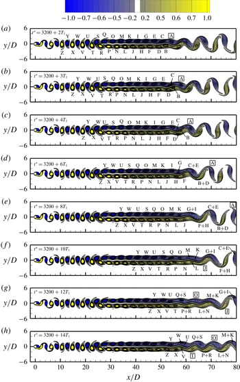
The time evolution of the vortices at
 $Re=300$
is illustrated by a typical sequence of the instantaneous vorticity fields shown in figure 13 (see also the online supplementary movie ‘Movie2.mp4’). The vorticity fields are shown at
 $t^{\ast }=3200+nT_{1}$
, where
 $n=2$
, 3, 4 and even integers up to 14. Based on flow visualisation, it is seen that the vorticity fields are highly repeatable for
 $x/D<45$
, which includes the first transition. Similar to the results of
 $Re=600$
shown in § 3, the range of
 $x/D$
for the highly repeatable flow is that in which the amplitude at
 $f_{2}$
is at least approximately one order of magnitude lower than that at
 $f_{1}$
(figure 12
b), such that the influence of
 $f_{2}$
is too weak to be visually detected.
A sequence of the instantaneous vorticity fields at
 $Re=300$
. The vorticity contours are shown from
 $-1$
to
 $+1$
with an interval of 0.1, plus
 $-0.64$
to
 $-0.56$
as well as 0.56–0.64 with an interval of 0.02 (to highlight the two-layered vortices near merging). The same vortices that appear in different snapshots are labelled with the same letters. The single vortices are marked by a rectangular frame around the vortex letter. The time evolution of the vorticity field can also be seen from the online supplementary movie ‘Movie2.mp4’ accompanying this article.

The vortices start to become irregular when they begin to rearrange themselves for the second transition. The second transition begins with the merging of two same-sign vortices (figure 13), rather than the pairing of two opposite-sign vortices as observed for
 $Re=600$
(figure 5). At
 $Re=300$
, when the two opposite-sign vortices (e.g. vortices B and C in figure 13
b) are about to pair, they are however not strong enough to break the restriction of the shear layer in between. Hence instead of pairing, they are each merged with the subsequent same-sign vortex directly (figure 13
c). Similar to the pairing and merging cycle for
 $Re=600$
, the merging of the same-sign vortices for
 $Re=300$
would also reduce the number of vortices by half. Therefore, a typical merging cycle for
 $Re=300$
also takes a period of approximately
 $2T_{1}$
.
The second merging cycle shown in figure 13(d) is similar to the first cycle shown in figure 13(b,c), while the third cycle shown in figure 13(e,f) is different. As vortices L and N merge together, vortex J is left out to be a single vortex. This phenomenon also happens for the subsequent two merging cycles, where single vortices O and T are observed in figure 13(g,h).
The moving location for the second transition for
 $Re=300$
originates from the moving location for the merging of the same-sign vortices shown in figure 13. In addition, the streamwise length occupied by the vortex merging process is not fixed. Compared with
 $Re=600$
, the flow at
 $Re=300$
is subjected to lower disturbance levels, such that vortex merging may not be triggered at the same streamwise location.
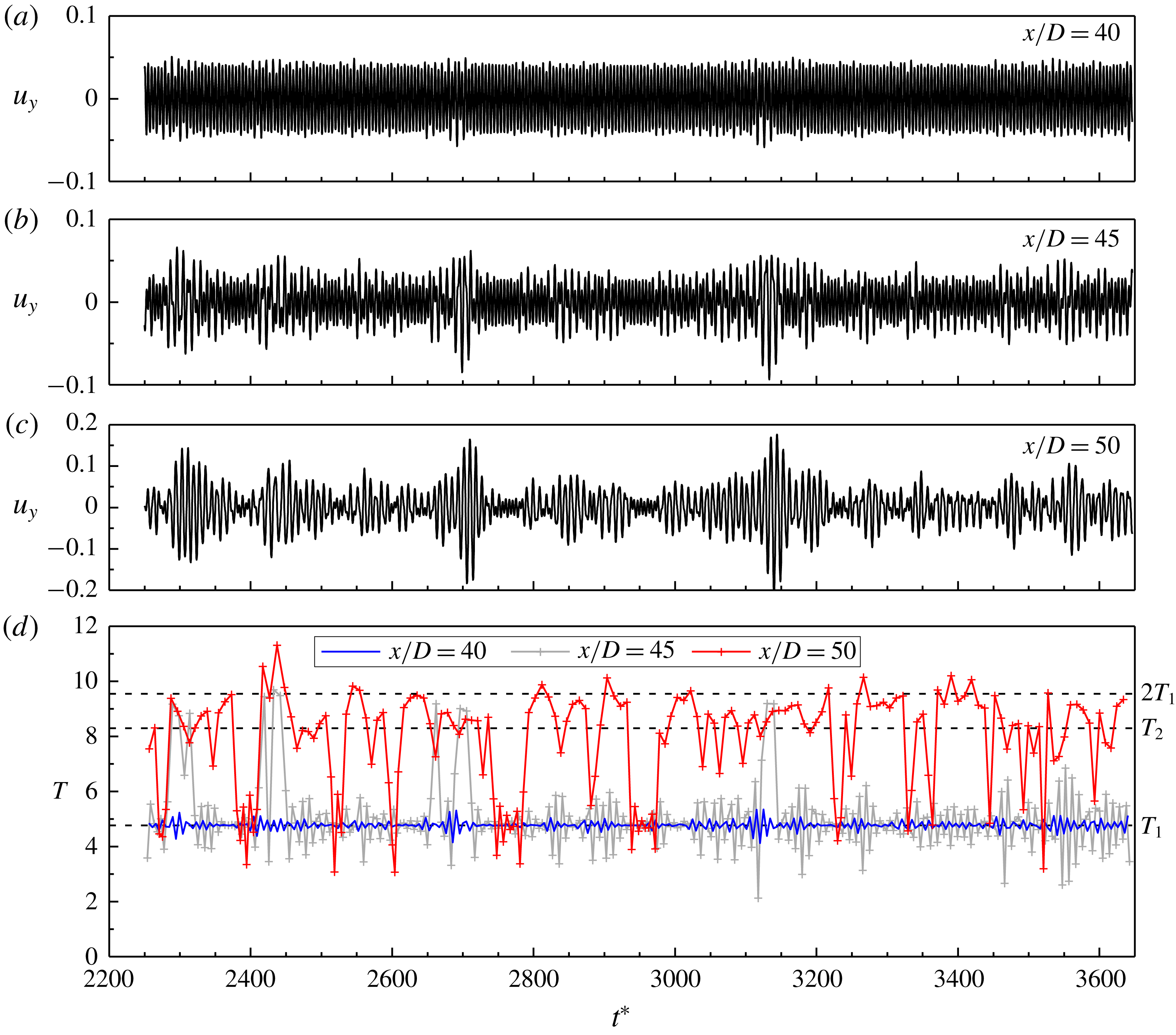
In addition to the flow visualisation in figure 13, the moving location for the vortex merging is also evidenced in figure 14 by the time histories of
 $u_{y}$
sampled in the wake. Figure 14(a–c) shows the time histories of
 $u_{y}$
sampled at
 $y=0$
and three streamwise locations, while figure 14(d) shows the period
 $T$
of each cycle of the time histories shown in figure 14(a–c). At
 $x/D=40$
, the two-layered vortices are highly repeatable with time since the amplitude of
 $u_{y}$
at
 $f_{2}$
is only 3.3 % of that at
 $f_{1}$
(figure 12
b). Therefore, the time history of
 $u_{y}$
shown in figure 14(a) is largely regular with time, and the periods are all very close to
 $T_{1}$
(figure 14
d). At
 $x/D=45$
, the amplitude at
 $f_{2}$
increases to 18.6 % of that at
 $f_{1}$
(figure 12
b). The amplitude at
 $f_{2}$
for the time history shown in figure 14(b) is intensively contributed by some short ranges of time, for example
 $t^{\ast }\sim 2700$
and 3130, rather than generally evenly contributed by the entire range of the time history (as is the case for
 $Re=600$
). For example, the FFT of the time history of
 $u_{y}$
over the short range of
 $t^{\ast }=2650$
–2730 gives the amplitude at
 $f_{1}$
identical to that shown in figure 12(b), but the amplitude at
 $f_{2}$
increased by approximately five times, reaching 93.8 % of that at
 $f_{1}$
. These short ranges of time are clearly identified in figure 14(d), where a drastic increase in the period from approximately
 $T_{1}$
to
 $2T_{1}$
is observed. These are the ranges of time when vortex merging happens closest to the cylinder. At
 $x/D=50$
, the amplitude at
 $f_{2}$
increases to 90.8 % of that at
 $f_{1}$
(figure 12
b), because more periods are increased from approximately
 $T_{1}$
to
 $2T_{1}$
(figure 14
d). Owing to the frequent generation of the single vortices, the periods after vortex merging are generally below
 $2T_{1}$
, which is similar to the results of
 $Re=600$
shown in figure 6(c). The remaining ranges of time, for example
 $t^{\ast }\sim 2770$
and 2960, are the ranges of time when vortex merging happens furthest away from the cylinder.
In contrast, for
 $Re=600$
the vortex pairing and merging process happens at a fixed streamwise location. Hence the time histories of
 $u_{y}$
shown in figure 6(a,b) do not contain sudden changes of the pattern with time. The amplitude of
 $u_{y}$
at
 $f_{2}$
for the time history shown in figure 6(b) is generally evenly contributed by the entire range of the time history rather than some short bursts.
Time histories of
 $u_{y}$
sampled at
 $y=0$
and
 $x/D=40$
(a), 45 (b) and 50 (c). In addition, panel (d) shows the period
 $T$
of each cycle of the time histories.

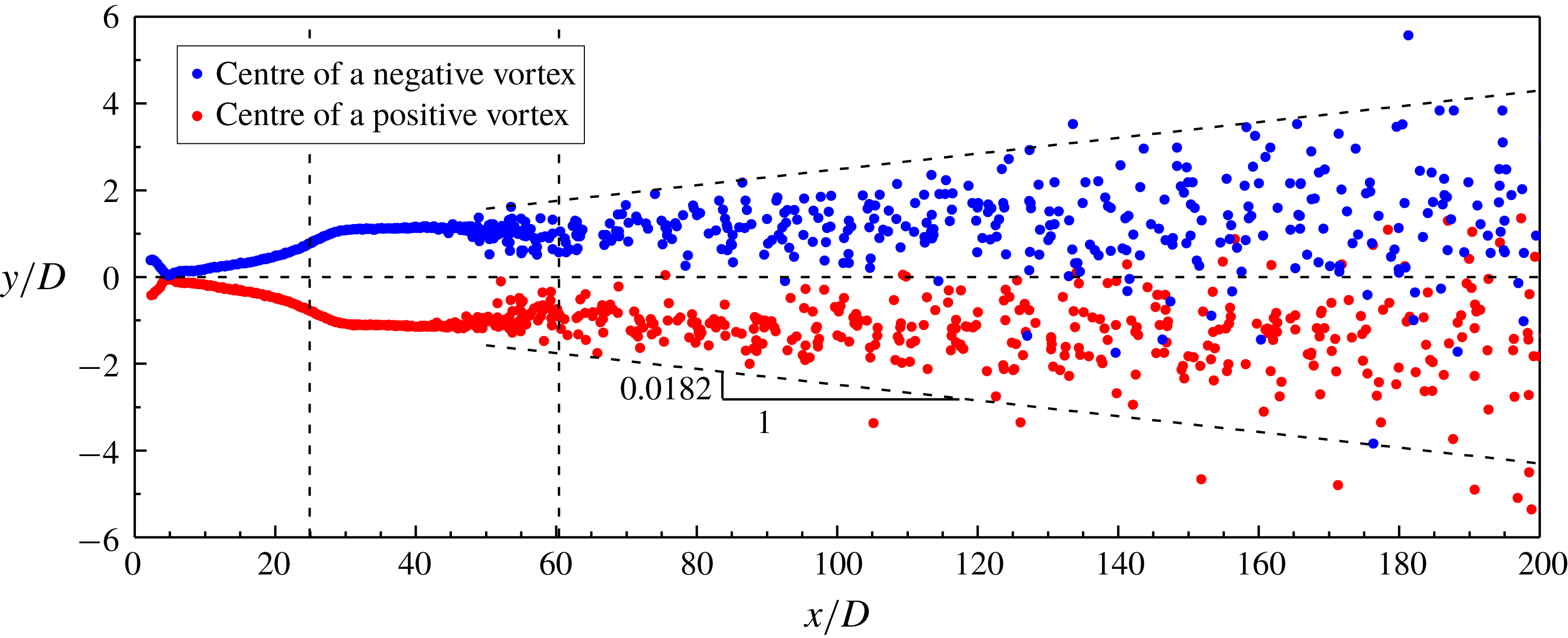
Spatial distribution of the vortex centres for
 $Re=300$
. The vertical dashed lines mark the two transition locations, while the horizontal dashed line marks the wake centreline. The inclined dashed lines mark the upper and lower envelopes for the majority of the vortex centres.

4.4 Irregularity of the flow
Figure 15 shows the spatial distribution of the vortex centres for
 $Re=300$
. The vortex centres are extracted from 19 snapshots of the vorticity field. Two clear trajectories for the centres of positive and negative vortices are observed for
 $x/D<45$
, while irregular spatial distributions of the vortices are observed for
 $x/D>45$
when they start to rearrange themselves for the irregular vortex merging process. The inclined dashed lines in figure 15 mark the upper and lower envelopes for the majority of the vortex centres (while extreme conditions may occur because at
 $Re=300$
the vortex merging process is highly irregular with time). The spatial expansion ratio is approximately
 $y:x=0.0182$
, which is approximately one-sixth of that at
 $Re=600$
(figure 7), since the vortices and vortex interactions are weaker at lower
 $Re$
values. Because of this slow transverse expansion, the positive and negative vortices generally stay in their respective half-domain up to
 $x/D\sim 120$
, which is much further downstream than the second transition location of
 $x/D=60.4$
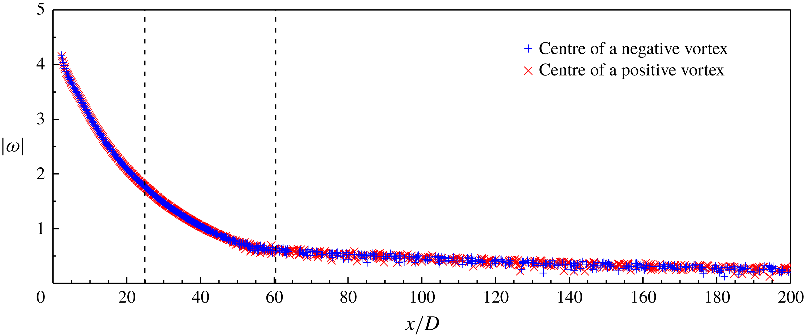
. Figure 16 shows the absolute value of the vorticity for the vortex centres identified in figure 15. As the vortices propagate downstream, the vorticity decays gradually. However, the decay rate is not linear. After the vortex centres display irregularity at
 $x/D>45$
(figure 15), slight scatters in the vorticity are observed in figure 16.
Absolute value of the vorticity at the vortex centre as a function of the streamwise location for
 $Re=300$
. The two transition locations are marked by the vertical dashed lines.

Figure 17 shows the variation of
 $c_{v}$
of the time history of
 $u_{y}$
(sampled at
 $y=0$
) with the streamwise location for
 $Re=300$
. For
 $x/D\leqslant 21$
, the
 $c_{v}$
values are smaller than 0.001, which suggests that the near-wake flow is perfectly time-periodic. A very slight increase in the
 $c_{v}$
value is observed at the first transition location, which suggests that the first transition is slightly aperiodic. The aperiodicity comes from a slight variation in the velocity amplitude, while the frequency is a single value. A major increase in the
 $c_{v}$
value is observed after
 $x/D=30$
, where
 $f_{2}$
emerges and increases in the amplitude with increase in
 $x/D$
. Different from the results at
 $Re=600$
, this major increase in
 $c_{v}$
for
 $Re=300$
is partly due to the moving location for the vortex merging process. For example, the large
 $c_{v}$
values observed at
 $x/D=45$
and 50 are due to a mixing of the pre- and post-merging
 $u_{y}$
signals (figure 14
b,c). With a further increase in the proportion of the post-merging
 $u_{y}$
signals, the
 $c_{v}$
value reduces gradually after
 $x/D=50$
. Eventually, as the secondary vortex street becomes increasingly irregular with distance downstream, an increase in the
 $c_{v}$
value is observed for
 $x/D>85$
.
Compared with flow visualisation, the irregularity of the flow is better detected by the
 $c_{v}$
value. For example, while the flow visualisations in figures 13 and 15 suggest that the flow is highly repeatable up to approximately
 $x/D=45$
, a large
 $c_{v}$
value is observed at
 $x/D=45$
(figure 17). This is partly because the flow irregularity is detected more sensitively by the time histories of the velocity components in the wake (e.g. figure 14) than flow visualisation, and partly because figures 13 and 15 may not always include the short ranges of time when vortex merging happens closest to the cylinder.
Variation of
 $c_{v}$
of the time history of
 $u_{y}$
(sampled at
 $y=0$
) with the streamwise location for
 $Re=300$
. The two transition locations are marked by the vertical dashed lines.

4.5 Results with a truncated wake
It has been indicated in §§ 4.3 and 4.4 that the amplitude of
 $u_{y}$
at
 $f_{2}$
and the flow irregularity in the two-layered vortex street are induced by the vortex merging process. These findings are further supported by an additional case with the computational domain truncated at
 $x/D=50$
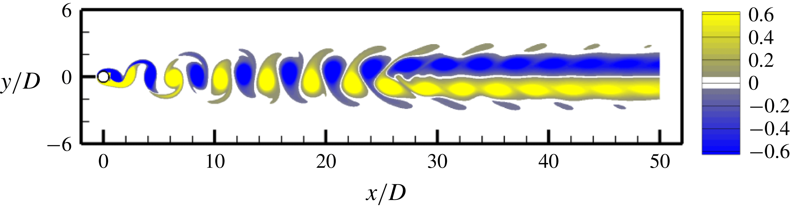
to exclude vortex merging. An instantaneous vorticity field of the fully developed flow is shown in figure 18. For this case, the time histories of
 $u_{y}$
sampled at various streamwise locations along both
 $y=0$
and
 $y=1$
are perfectly time-periodic, with the
 $c_{v}$
values smaller than
 $10^{-4}$
, which indicates that the flow is perfectly time-periodic. In particular, the
 $c_{v}$
value at the location of the first transition remains below
 $10^{-4}$
, which suggests that the slightly aperiodic first transition indicated in figure 17 is also induced by vortex merging.
Instantaneous vorticity field of the fully developed flow for
 $Re=300$
at
 $t^{\ast }=3900$
with the computational domain truncated at
 $x/D=50$
.

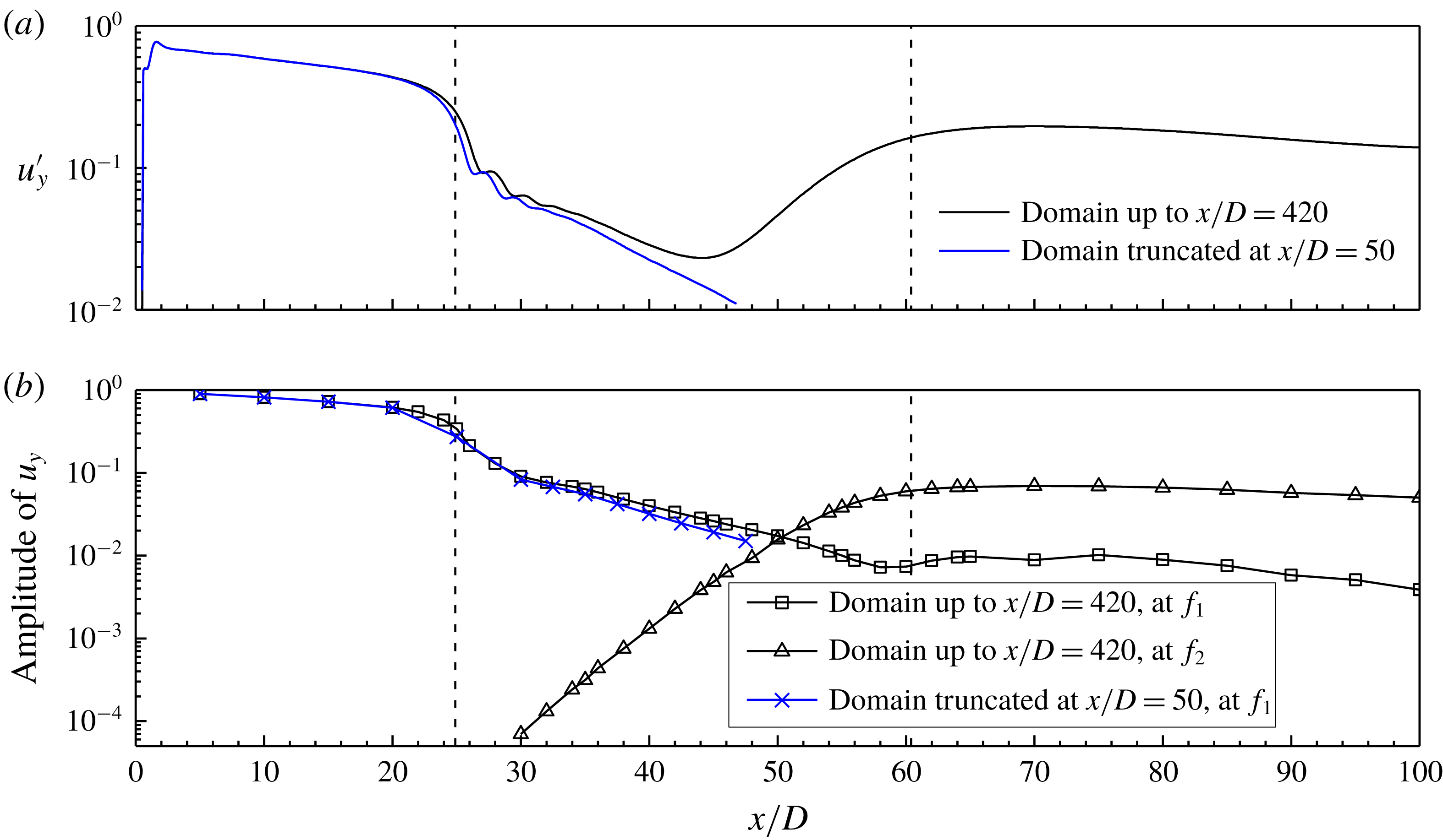
Figure 19 shows the amplitude of
 $u_{y}$
in the wake (sampled at
 $y=0$
) for the case with the truncated domain, together with the results with a sufficiently long domain up to
 $x/D=420$
(with the results adapted from figure 12
a,b). Figure 19(a) shows that without the influence of the second transition an exponential decay of the
 $u_{y}^{\prime }$
value is observed for
 $x/D>34$
for the truncated case. The slightly smaller
 $u_{y}^{\prime }$
values for the truncated case result in slightly smaller amplitudes at
 $f_{1}$
(figure 19
b). For the truncated case, only a single frequency value
 $f_{1}$
is observed in the frequency spectra of
 $u_{y}$
. The absence of
 $f_{2}$
for the truncated case proves that the
 $f_{2}$
signal detected in the two-layered vortex street indeed originates from vortex merging.
Variation of the amplitude of
 $u_{y}$
(sampled at
 $y=0$
) with the streamwise location for
 $Re=300$
. The amplitude of
 $u_{y}$
is examined with (a) root-mean-square of
 $u_{y}$
, and (b) amplitude of
 $u_{y}$
at the two frequencies
 $f_{1}$
and
 $f_{2}$
. The two transition locations are marked by the vertical dashed lines.

5 Results for
$Re=150{-}1000$

5.1 The transition locations
The flow characteristics for
 $Re=150$
–1000 are summarised in this section. The transition locations for
 $Re=150$
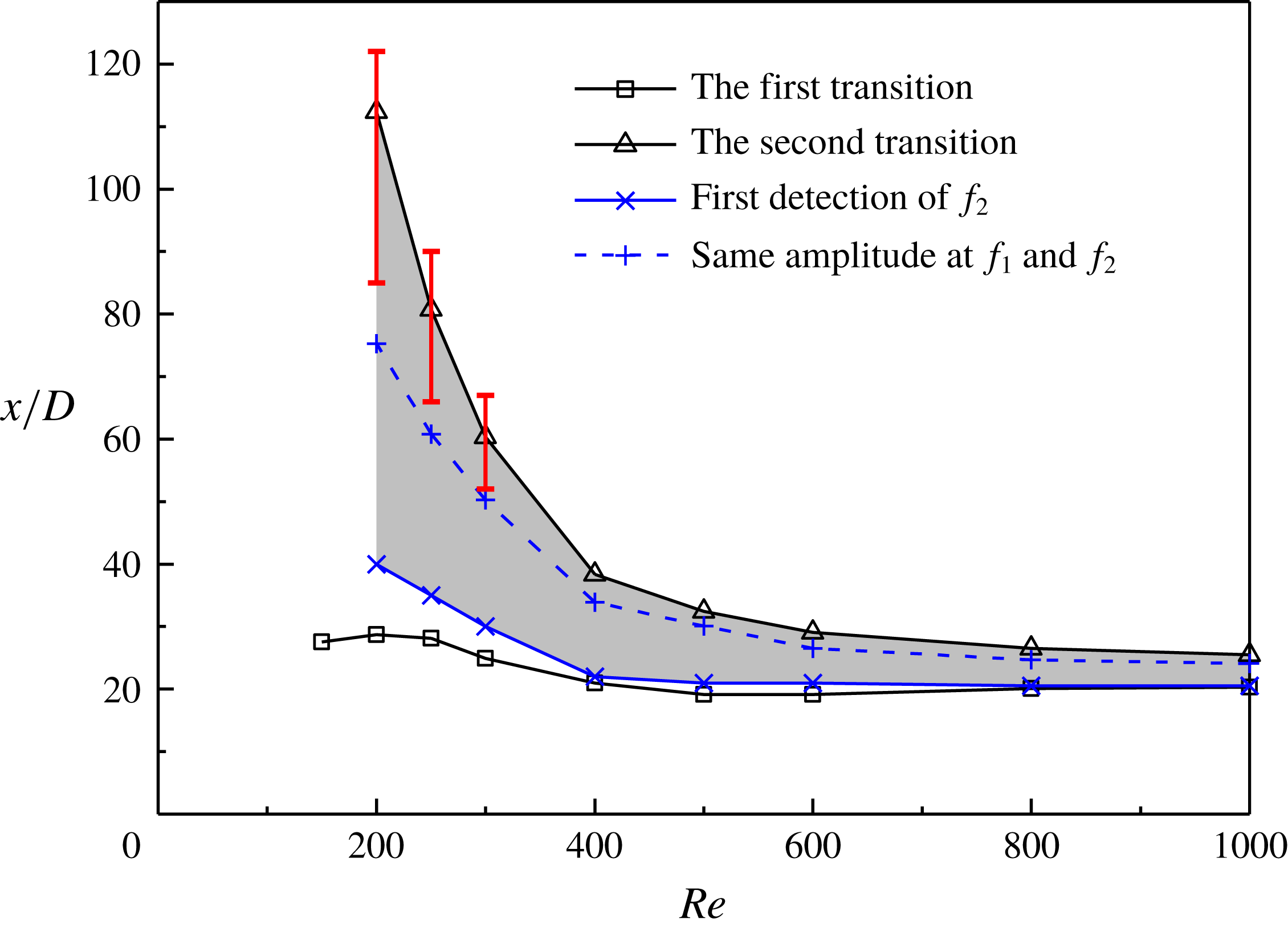
–1000, which are determined based on the time-averaged transverse velocity field, are shown in figure 20. The first transition occurs within a small range of approximately
 $x/D=20$
–30. The second transition moves upstream significantly with increasing
 $Re$
, as is also observed in Inoue & Yamazaki (Reference Inoue and Yamazaki1999) and Vorobieff et al. (Reference Vorobieff, Georgiev and Ingber2002).
Transition locations determined based on the time-averaged transverse velocity field. The red vertical bars indicate approximate ranges for the movement of the second transition location over time.

It is noted that the transition locations shown in figure 20 represent time-averaged results. In addition, the time evolution of the flow is checked through flow visualisation. For
 $Re\geqslant 400$
, both transition locations do not vary with time. For
 $Re\leqslant 300$
, the first transition location is stationary while the second moves back and forth in time. The moving location for the second transition originates from the moving location for the merging of the same-sign vortices and a varying streamwise length occupied by the vortex merging process. The red vertical bars shown in figure 20 indicate approximate ranges for the movement of the second transition location over time. The range of movement increases with decreasing
 $Re$
.
5.2 Frequencies in the wake
As illustrated in figure 4(b,c) for
 $Re=600$
and figure 12(b,c) for
 $Re=300$
, the
 $f_{2}$
signal is first detected in a short streamwise distance after the first transition. Figure 20 summarises the streamwise locations for the first detection of
 $f_{2}$
for
 $Re=200$
–1000. For
 $x/D$
from the first detection of
 $f_{2}$
to the second transition (the shaded range in figure 20), there is a gradual changeover in the normalised amplitude of
 $u_{y}$
from
 $f_{1}$
to
 $f_{2}$
(e.g. figures 4
c and 12
c). The streamwise location for the same amplitude at
 $f_{1}$
and
 $f_{2}$
is also shown in figure 20. The
 $f_{1}$
-dominated range is larger than the
 $f_{2}$
-dominated range. This is because, when
 $f_{2}$
is first detected, its amplitude is only approximately
 $1\times 10^{-4}$
–
 $1\times 10^{-3}$
, and it takes a certain streamwise distance for the amplitude to grow over a few orders of magnitude.
The frequency spectra of
 $f_{2}$
for
 $Re=200$
–1000 are governed by the pairing and merging of the two-layered vortices. With increasing
 $Re$
, the pairing and merging of vortices become increasingly regular with time. At relatively low
 $Re$
of 200–300, the irregular movement of the streamwise location for the vortex merging and the irregular generation of the single vortices lead to large variations in the periods of the time histories of
 $u_{y}$
(e.g. figure 14
d), which result in broad-band frequency spectra of
 $f_{2}$
(e.g. figure 11). In contrast, for
 $Re=400$
–1000 the vortex pairing and merging process happens at a fixed streamwise location. Hence the periods of the time histories of
 $u_{y}$
(e.g. figure 6
c) are mainly concentrated in a relatively small range, and a sharp
 $f_{2}$
peak is observed in the frequency spectra (e.g. figure 3). For
 $Re=400$
–600, the sharp
 $f_{2}$
peak is accompanied by small-scale broad-band frequencies at the two sides of the peak (e.g. figure 3), because the irregular generation of the single vortices would result in irregular local reductions in the periods of the time histories of
 $u_{y}$
(e.g. figure 6
c). For
 $Re=800$
–1000, the generation of the single vortices becomes more regular with time. For example, an examination of the time evolution of the flow at
 $Re=1000$
over 94 primary vortex shedding cycles shows that there are 34 pairing and merging cycles, and each cycle is accompanied by one or two single vortices in the pattern of (i) a positive single vortex, (ii) a negative single vortex, or (iii) positive and negative single vortices. The patterns for each of the 34 pairing and merging cycles are summarised in figure 21. The shaded and clear grids indicate the existence and absence of a single vortex, respectively. The absence of a positive/negative single vortex generally happens every four to five cycles. In addition, figure 21 contains three identical ranges that repeat every nine cycles. The largely regular generation of the single vortices results in a sharp
 $f_{2}$
peak in the frequency spectrum with hardly any broad-band frequencies at the two sides (figure 22). Without the influence of the broad-band frequencies, some harmonics of
 $f_{1}$
and
 $f_{2}$
are also identified.
Single vortex pattern for each of the 34 pairing and merging cycles observed at
 $Re=1000$
.

Frequency spectrum of
 $u_{y}$
sampled at
 $(x/D,y/D)=(26,0)$
for
 $Re=1000$
. The frequency spectrum is calculated from the FFT of the time history of
 $u_{y}$
over a period of 199 primary vortex shedding periods.

Because the merging of the two-layered vortices is accompanied by frequent generation of the single vortices, the peak frequency
 $f_{2}$
for
 $Re=400$
–1000 and the majority of the broad-band range of
 $f_{2}$
for
 $Re=200$
–300 are larger than
 $0.5f_{1}$
. For
 $Re=400$
–1000,
 $f_{2}$
in the frequency spectra is determined by the number of vortices observed in the flow through the following expression:
 $$\begin{eqnarray}\frac{f_{2}}{\,f_{1}\,}=\frac{\text{number of vortices after the merging}}{\text{ number of vortices before the merging }}.\end{eqnarray}$$
For example, table 1 lists the numbers of vortices observed before and after the merging for certain non-dimensional time units for
 $Re=400$
, 600 and 1000. The results shown in table 1 satisfy equation (5.1).
Numbers of vortices observed before and after the merging for certain non-dimensional time units.

6 Conclusions
This study examines the two-dimensional (laminar) flows in the intermediate and far wake of a circular cylinder for
 $Re=150$
–1000. The streamwise locations for the first and second transitions are determined by the time-averaged transverse velocity field. By examining the time evolution of the flow, it is found that the location for the first transition is stationary while the location for the second transition may move with time at relatively low
 $Re$
values. The range of movement increases with decreasing
 $Re$
.
Two processes for the second transition are observed. For relatively large
 $Re=400{-}1000$
, the second transition is an irregular pairing and merging process, which begins with the pairing of two opposite-sign vortices, followed by the merging of the paired vortices into two subsequent vortices. For relatively small
 $Re=200{-}300$
, the second transition begins with the merging of two same-sign vortices, since the opposite-sign vortices are not strong enough to break the restriction of the shear layer in between and to pair. For both conditions, single vortices may be generated between the irregular merging cycles due to mismatch of the vortices.
The location for the second transition moves back and forth in time for
 $Re=200$
–300, which originates from the movement of the location of the vortex merging process (while the streamwise location for the pairing and merging process for
 $Re=400$
–1000 is stationary). Since the flow at lower
 $Re$
is subjected to lower disturbance levels, vortex merging may not be triggered at the same streamwise location.
In addition to the primary vortex shedding frequency
 $f_{1}$
, another frequency peak/range
 $f_{2}$
is detected in a short streamwise distance after the first transition. From the emergence of
 $f_{2}$
to the second transition, there is a gradual increase in the normalised amplitude at
 $f_{2}$
and a corresponding gradual decrease in the normalised amplitude at
 $f_{1}$
. The
 $f_{2}$
signal and the flow irregularity in the two-layered vortex street for
 $Re=200$
–1000 are induced by the irregular pairing and merging of the two-layered vortices. The broad-band frequency spectra of
 $f_{2}$
for
 $Re=200$
–300 are due to the irregular movement of the streamwise location for the vortex merging and the irregular generation of the single vortices. The frequency spectra of
 $f_{2}$
become increasingly sharp-peaked for
 $Re=400$
–1000 because the vortex pairing and merging process happens at a fixed streamwise location, and the generation of the single vortices becomes increasingly regular with increasing
 $Re$
. Owing to the generation of single vortices between the pairing and merging cycles, the peak frequency
 $f_{2}$
is larger than 0.5
 $f_{1}$
. The ratio of
 $f_{2}$
and
 $f_{1}$
is equal to the ratio of the numbers of vortices observed after and before the merging.
Acknowledgements
The authors would like to acknowledge the support from the National Key R&D Program of China (Project ID: 2016YFE0200100) and from the Australian Research Council through LP150100249. The first author would like to acknowledge the support from the Australian Research Council through DECRA Schemes (DE190100870). This work was supported by resources provided by the Pawsey Supercomputing Centre with funding from the Australian Government and the Government of Western Australia.
Supplementary movies
Supplementary movies are available at https://doi.org/10.1017/jfm.2019.167.
Appendix A. Mesh convergence
The streamwise location of the second transition reported in the literature showed large scatters. For example, based on two-dimensional numerical simulations, Vorobieff et al. (Reference Vorobieff, Georgiev and Ingber2002) and Kumar & Mittal (Reference Kumar and Mittal2012) observed the second transition for
 $Re=200$
at approximately
 $x/D=60$
and 100, respectively, while Thompson et al. (Reference Thompson, Radi, Rao, Sheridan and Hourigan2014) did not observe the secondary vortex street at
 $Re=200$
up to a wake domain length of
 $x/D=280$
. The large scatters of the transition location reported in the literature motivate a detailed mesh independence check.
In addition to a variation of the order of polynomial expansions for the macro-element mesh in the framework of
 $\text{Nektar}++$
(where the cases are referred to as, for example, Nektar–
 $N_{p}=5$
), cross-checks are carried out by using another open-source code, OpenFOAM (http://www.openfoam.org), that is based on the finite volume method. In the framework of OpenFOAM, the numerical methodology is the same as that used in Jiang et al. (Reference Jiang, Cheng, Draper, An and Tong2016) and Jiang & Cheng (Reference Jiang and Cheng2017) for the simulations of the near-wake flow of a circular cylinder. Two meshes, which are referred to as OpenFOAM–1 and OpenFOAM–2, are used. OpenFOAM–1 is based on the ‘refined mesh’ used in Jiang & Cheng (Reference Jiang and Cheng2017) for
 $Re$
up to 1000, where the cylinder perimeter is discretised with 240 cells, the radial size of the first layer of mesh next to the cylinder is
 $2.315\times 10^{-4}\,D$
, but the computational domain size is enlarged to be identical to the one used in
 $\text{Nektar}++$
(
 $-60\leqslant x/D\leqslant 420$
and
 $-60\leqslant y/D\leqslant 60$
), and the wake region is refined by specifying the streamwise size of the mesh at the wake centreline varying linearly from
 $0.0375D$
at
 $x/D=2$
to
 $2.5\times 0.0375D$
at
 $x/D=400$
. OpenFOAM–2 is a further refinement of OpenFOAM–1, with a doubled number of cells in both
 $x$
- and
 $y$
-directions, while the general topology remains the same. In particular, the number of cells around the cylinder perimeter is doubled from 240 to 480, the radial size of the first layer of mesh next to the cylinder is halved from
 $2.315\times 10^{-4}\,D$
to
 $1.174\times 10^{-4}\,D$
, and the streamwise size of the mesh at the wake centreline is halved to a linear variation of
 $0.01875D$
at
 $x/D=2$
to
 $2.5\times 0.01875D$
at
 $x/D=400$
.
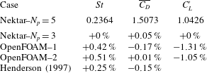
First, table 2 lists the hydrodynamic forces on the cylinder at
 $Re=1000$
(the largest
 $Re$
adopted in this study) calculated with different meshes. The drag and lift coefficients (
 $C_{D}$
and
 $C_{L}$
) and the Strouhal number (
 $St$
) are defined as follows.
 $$\begin{eqnarray}\displaystyle & \displaystyle C_{D}=\frac{F_{D}}{\frac{1}{2}\unicode[STIX]{x1D70C}U^{2}D}, & \displaystyle\end{eqnarray}$$
 $$\begin{eqnarray}\displaystyle & \displaystyle C_{L}=\frac{F_{L}}{\frac{1}{2}\unicode[STIX]{x1D70C}U^{2}D}, & \displaystyle\end{eqnarray}$$
 $$\begin{eqnarray}\displaystyle & \displaystyle St=\frac{F_{L}D}{U}, & \displaystyle\end{eqnarray}$$
where
 $F_{D}$
and
 $F_{L}$
are the drag force and lift force on the cylinder, respectively, and
 $f_{L}$
is the frequency of the fluctuating lift force. The time-averaged drag coefficient
 $(\overline{C_{D}})$
and the root-mean-square lift coefficient
 $(C_{L}^{\prime })$
are calculated as
 $$\begin{eqnarray}\displaystyle & \displaystyle \overline{C_{D}}=\frac{1}{N}\mathop{\sum }_{i=1}^{N}C_{D,i}, & \displaystyle\end{eqnarray}$$
 $$\begin{eqnarray}\displaystyle & \displaystyle C_{L}^{\prime }=\sqrt{\frac{1}{N}\mathop{\sum }_{i=1}^{N}(C_{L,i}-\overline{C_{L}})^{2}}, & \displaystyle\end{eqnarray}$$
where
 $N$
is the number of values in the time history. As shown in table 2, very good agreements in the hydrodynamic forces are observed for all the cases, even when using relatively coarse meshes such as Nektar–
 $N_{p}=3$
and OpenFOAM–1. The mesh convergence of the hydrodynamic forces on the cylinder demonstrates the quality of the mesh close to the cylinder.
Mesh independence check of the hydrodynamic forces on the cylinder at
 $Re=1000$
. The results other than the case Nektar–
 $N_{p}=5$
are shown by the relative differences with respect to those of Nektar–
 $N_{p}=5$
.

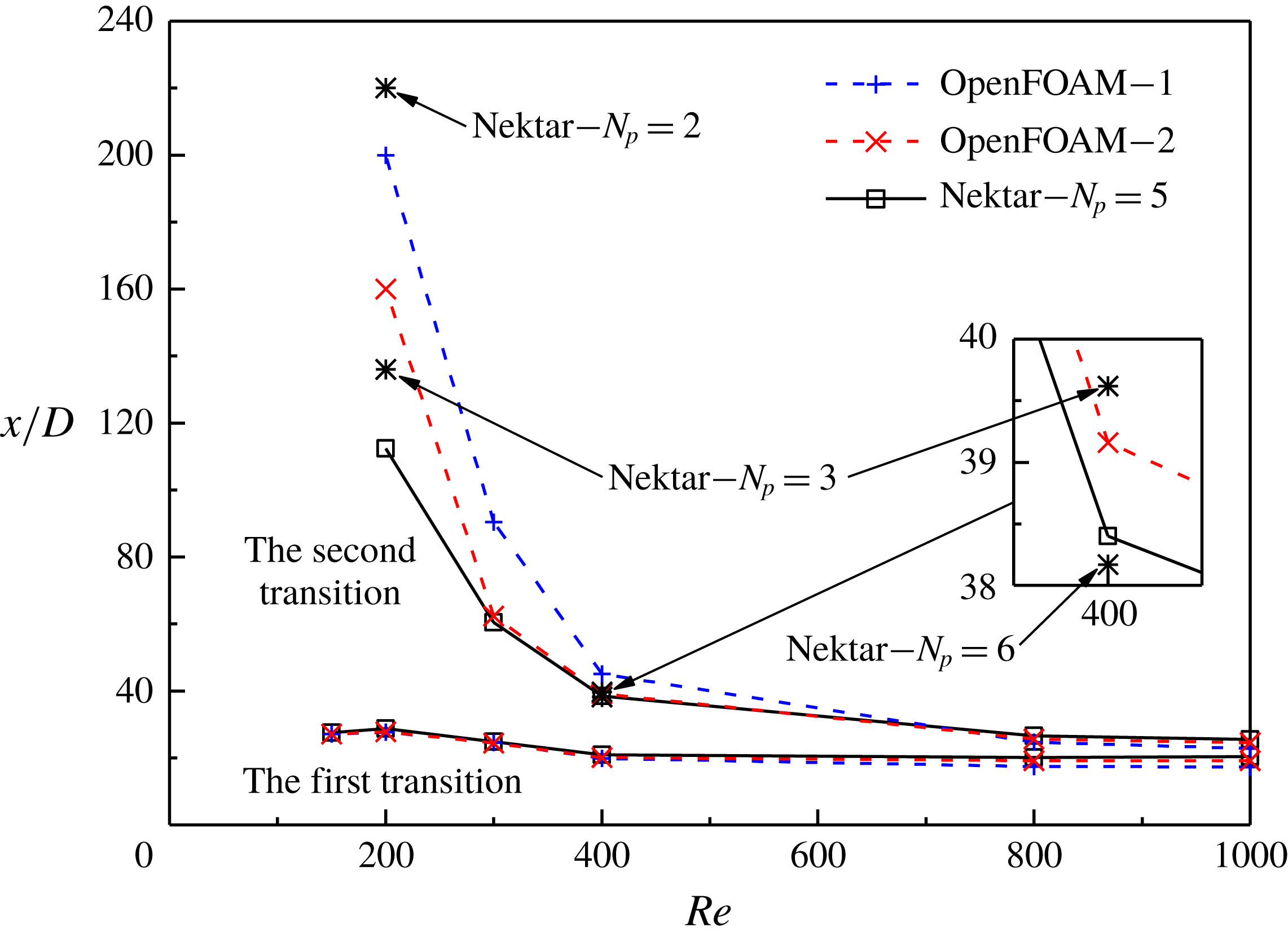
Next, the mesh resolution in the far wake is checked by examining the streamwise location of the second transition (where large scatters exist in the literature). Figure 23 shows the two transition locations for various
 $Re$
values determined by different meshes. The method for the determination of the transition locations is introduced in § 3.1. As shown in figure 23, good agreements are observed at the first transition, while differences exist at the second one, as outlined below.
(i) With a refinement of the mesh resolution from OpenFOAM–1 to OpenFOAM–2, the second transition moves upstream for
$Re=200$
–400 but moves slightly downstream for
$Re=800$
and 1000. This is because the disturbance level at the second transition is influenced by two numerical aspects with opposite effects. The first aspect is the numerical disturbance generated in the computational domain (e.g. at the locations of mesh skewness; see figure 1), which reduces with increasing mesh resolution. The second aspect is the streamwise convection of the numerical disturbance to the far wake, which is less dissipative with increasing mesh resolution. As shown in figure 23, the results at
$Re=200$
–400 are dominated by the dissipation of the disturbance, while the results at
$Re=800$
and 1000 are dominated by the generation of the disturbance.(ii) The results calculated with OpenFOAM–1 and OpenFOAM–2 show that the location of the second transition is most mesh-dependent at the smallest
$Re$
of 200, rather than at the largest
$Re$
of 1000. Further results at
$Re=200$
and 400 calculated with
$\text{Nektar}++$
with different
$N_{p}$
values suggest that an
$N_{p}$
of 5 should be sufficient for the present study.(iii) For
$Re=300$
–1000, excellent agreements are observed for the results calculated with OpenFOAM–2 and Nektar–
$N_{p}=5$
, which suggests that both computational codes produce reliable results.


The two transition locations for various
 $Re$
values determined by different meshes.

Modified macro-element mesh with an additional layer of macro-elements of doubled streamwise size of
 $2\times 0.1875D$
at
 $x/D\sim 2$
.

It is also noticed that the streamwise location for the second transition may be sensitive to large variations in the size of the neighbouring macro-elements near the cylinder. This phenomenon is most pronounced for the most mesh-dependent case of
 $Re=200$
. For example, by using a mesh slightly modified from figure 1 with an additional layer of macro-elements of doubled streamwise size of
 $2\times 0.1875D$
at
 $x/D\sim 2$
(figure 24), the streamwise location for the second transition calculated with
 $N_{p}=3$
is delayed significantly from
 $136D$
downstream of the cylinder to more than
 $250D$
downstream of the cylinder. Such a delay in the second transition is possibly due to an increased numerical dissipation at the sudden expansion of the mesh size. Therefore, care has been taken in the construction of the macro-element mesh shown in figure 1 to ensure a gradual variation in the macro-element size near the cylinder. A well-constructed macro-element mesh would lessen the demand for the order of polynomial expansions.