I. INTRODUCTION
Indentation techniques have become a standard method to assess the mechanical properties of numerous materials.Reference Willems, Celis, Lambrechts, Braem and Vanherle1, Reference Turner, Rho, Takano, Tsui and Pharr2 In recent years, nanoindentation of bone has been used to extract the mechanical behavior at the level of osteons,Reference Hoc, Henry, Verdier, Aubry, Sedel and Meunier3, Reference Zhang, Niebur and Ovaert4 or even lamellae.Reference Hoffler, Guo, Zysset and Goldstein5 Different procedures during the indentation test can be used for different testing purposes. A conventional test provides the hardness of materials by measuring the size of the residual indentation impression. The load and indentation depth can also be recorded to form an indentation curve, which reveals information regarding mechanical properties. There are many material models for bone, reflecting its anisotropic structure.Reference Siegmund, Allen and Burr6 On large scales and small strain levels, bone can be modeled as viscoelastic,Reference Zhang, Niebur and Ovaert4, Reference Hoffler, Guo, Zysset and Goldstein5, Reference Bembey, Oyen, Bushby and Boyde7, Reference Isaksson, Nagao, Małkiewicz, Julkunen, Nowak and Jurvelin8 viscoelastic-plastic,Reference Oyen and Ko9 or elastic-plastic damage.Reference Garcia, Zysset, Charlebois and Curnier10 At reduced (micron) scales, cortical bone consists of osteons embedded in interstitial bone,Reference Hoc, Henry, Verdier, Aubry, Sedel and Meunier3 while trabecular bone consists of structures similar to rods or plates. Continuum models on the micron scale can represent the overall behavior during indentation, regardless of the anisotropic microstructure and interactions within the microstructure. However, at the nanoscale, indentation becomes much more localized, where the structure of interest can be collagen and the mineral crystals that bond it together.Reference Ji11
Under a fluorescent light microscope, tiny microcracks can be observed in cortical bone and breaking of trabeculae can be observed in trabecular bone, which have been implicated in physiological phenomena including stress fractures, bone remodeling, and adaptation.Reference Ramtani and Zidi12 These material discontinuities can also be considered as damage. To account for the damage effect of bone for modeling bone indentation behavior, one needs to differentiate two irreversible processes: damage and plasticity. Mathematically, damage represents the gradual degradation of elastic modulus, while plasticity represents the development of irreversible permanent strains. Physiologically, damage may be caused by the breaking of bonds and plasticity by material dislocations.Reference Souchet13 The concept of dislocations is well accepted for metals; however, this is not the case for bone. From a physical point of view, the breaking of bonds can be due to growths of microdefects such as cracks and voids, while dislocations are due to elementary slippage along interfaces.Reference Souchet13 Damage accumulation in bone is generated through daily mechanical loading, and bone quality is degraded during this process, which is then recovered during to the process of remodeling. Poor bone quality is one cause of osteoporosis, which can lead to bone fractures.Reference Ager, Balooch and Ritchie14 For bone indentation modeling, though pre-existing damage may be omitted in most cases, new damage can also be produced during the process of testing, particularly using sharp-tipped indenters. Thus, damage accumulation should be considered when establishing an indentation bone model, especially in high load (mN-scale) cases, where damage is readily evident.
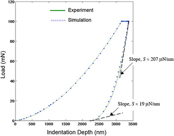
Recently, an Abaqus concrete plastic-damage material model was applied to simulate bone indentation by Zhang et al.Reference Zhang, Michalenko, Kuhl and Ovaert15 A “softening” behavior in the tail region of the unloading curve was observed in a typical load versus indentation depth creep experiment. It was hypothesized that this stiffness reduction in bone is due to damage, rather than thermal drift. The concrete plastic-damage model accurately simulated the characteristic indentation response of bone for the loading, holding, and unloading stages. The result is shown in Fig. 1.
Load versus indentation depth curve (from Zhang et al.15) showing stiffness reduction at the end of unloading and agreement between simulation using Abaqus concrete plastic damage model and bone experimental data.

This plastic-damage model, however, is primarily intended to provide the capability for modeling concrete structures and other quasi-brittle materials. A more detailed mathematical description of the concrete plastic-damage model can be found in the Abaqus Theory Manual.16 The model requires the specification of 13 parameters, including parameters that account for concrete’s tensile properties. Since indentation loading is predominantly a compression event, the parameter set may be simplified somewhat when the tensile strains are small. A further problem using this model is the fact that most of the parameters have not been systematically defined for bone.
The identification of material parameters using a combination of indentation experiments, finite element analysis, and optimization methods has been accomplished by a number of researchers.Reference Liu and Ovaert17–Reference Galli, Fornasiere, Cugnoni and Oyen20 However, even the simplified concrete plastic-damage model is still complex mathematically and does not easily lend itself to optimization methods for parameter determination. The issues have to do with the sensitivities of the optimized objective function to the parameter set (minimization of the error between the experimental and simulated load versus indentation depth curves), the number of parameters, and the initial parameter set values. Finally, treating a hierarchically complex material such as bone, using the mechanics developed for concrete, is a difficult task in itself.
Therefore, the objective of this research is to establish a more general and simplified viscoelastic-plastic damage model that contains fewer material parameters, yet can still successfully capture the characteristics of bone nanoindentation behavior. In what follows, we will describe the mathematical and finite element formulation of the model, applied via Abaqus as a user-defined subroutine (UMAT) in conjunction with the Matlab optimization toolbox. A parametric sensitivity study is also performed to better understand the sensitivity of the indentation response to the parameters in the model. Finally, the model was applied to simulate the indentation creep response of sheep bone samples at baseline and OVX-2 to elucidate the potential difference in damage progression between the two groups.
II. METHODOLOGY
A. Viscoelastic-plastic damage model
A typical nanoindentation creep curve contains loading, holding, and unloading segments. After indentation, the following characteristics can be observed from a load versus indentation depth plot of bone: a residual deformation exists after the load is removed, which implies that bone deforms permanently, and when the load is held constant after first reaching the maximum load, the indentation depth continues to increase, thus, bone is also viscoelastic. Therefore, to establish a damage model that can simulate the indentation behavior of bone, it must also include the constitutive properties of plasticity and viscoelasticity.
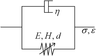
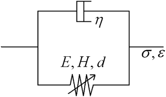
The viscoelastic-plastic damage model that we established via a user-defined material model (UMAT) consists of a damaged elasto-plastic spring in parallel with a linear dashpot, as shown in Fig. 2. Thus, the damage model is the simplest material model that includes the mechanical properties of elasticity (E), viscoelasticity (η), plasticity (H), and damage (d, modeled using the parameters γ and β).
Viscoelastic-plastic damage model used in the finite element simulations.
The stress–strain relationship in the damage model is given as:


where the superscript “s” denotes the spring and “d” denotes the dashpot.
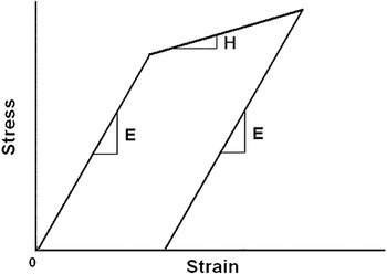
The spring is responsible for the material properties of elasticity and plasticity, having an effective stress–strain curve shown in Fig. 3. In the elastic region, the constitutive law takes the simple linear elastic form as:

Stress–strain curve for elastic-linear hardening material.

where E is Young’s modulus. The three-dimensional (3D) form is given by:

where 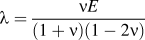 ,
 , and ν is Poisson’s ratio.
To simulate permanent deformation, J2 plasticity is used. In one dimension, it takes the form of a linear hardening model. Thus, we use a single parameter H, the slope of the stress–strain curve (assumed linear, Fig. 3) after yielding, to quantify plasticity. The parameter Y is the yield strength of bone.
In three dimensions, the yield function, plastic strain, and the flow law are defined in the following equations:
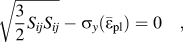
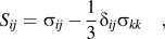
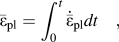
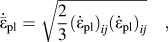
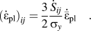
The effective stress  is related to the true stress σ by:

Here the scalar damage parameter, d, is used to specify the effect of damage, and (1 – d) represents the undamaged area fraction. Also, d = 0 defines zero damage and d = 1 defines complete damage. In this case, d satisfies 0 ≤ d ≤ 1.
In general, there are various ways to define the damage evolution equation. Here, we use a simple model that relates the damage parameter solely to the equivalent plastic strain:

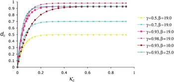
where d is the damage parameter; κ is the equivalent plastic strain; γ specifies the limiting value of damage; and β specifies the damage initiation rate. The model implies that damage initiates after the yield point is reached. With some assumed values of γ and β, the damage evolution equation can be plotted as shown in Fig. 4.
Damage parameter, d c, as a function of the equivalent plastic strain, κ c (where subscript “c” refers to compression), for various values of γ and β (from Zhang et al.Reference Garcia, Zysset, Charlebois and Curnier15).

For the dashpot, the one-dimensional (1D) governing equation is given by:

In three dimensions, the equation can be written in matrix form as:
where the viscosity η is divided into a volumetric part η v and a deviatoric part η d:

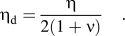
In the Abaqus UMAT, the Jacobian matrix must be provided at the end of each step. In our case, the Jacobian matrix is the sum of the spring and the dashpot stiffness matrices

where the Jacobian matrix itself is defined as:

Thus, the simplified viscoelastic-plastic damage model contains six material parameters E (modulus), H (slope of the plastic stress–strain curve), Y (yield strength), γ (damage-limiting parameter), β (damage initiation parameter), and η (viscosity), with Poisson’s ratio fixed at 0.3 for bone as noted elsewhere.Reference Zhang, Niebur and Ovaert4
B. Experimental
Normal and osteoporotic sheep trabecular bone samples were harvested from the distal femur and tested via nanoindentation. Sample I was baseline, and sample II was 24-month postovariectomy (OVX-2). The nanoindentation was performed using a Hysitron TriboIndenter (Eden Prairie, MN) with a Berkovich indenter on hydrated specimens detailed previously.Reference Wu, Baker, Ovaert and Niebur21 The maximum load was 10 mN, the loading/unloading rate was 2 mN/s, and the hold time was 30 s. Indents were performed on each sample as to obtain averaged properties of the sample (approximately 40 indents per sample). The average Young’s modulus was calculated for each indent using the Oliver–Pharr method. Then for each sample, five distinct indentation curves whose Young’s modulus was closest to the average Young’s modulus of the sample were selected as the representative curves of the sample. The five creep curves were then averaged to obtain a single “experimental” curve representative of the average indentation response of the sample. In addition, the tissue mineral density (TMD) for each sample was obtained using micro-CT following the method of Bouxsein et al. and others,Reference Bouxsein, Boyd, Christiansen, Guldberg, Jepsen and Muller22, Reference Kazakia, Burghardt, Cheung and Majumdar23 as the state of osteoporosis is mainly determined by TMD.
C. Finite element formulation
The viscoelastic-plastic damage model was implemented in Abaqus. The mechanical properties of each sample were obtained by minimizing the error between the simulation indentation curve and averaged experimental curve. The damage evolution equation for each sample was also plotted.
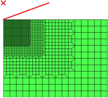
The axisymmetric finite element model is shown in Fig. 5. The diamond Berkovich indenter used in the nanoindentation test was modeled as a 70.3° cone, represented in Fig. 5 in the upper left-hand corner. One thousand seven hundred and forty-three axisymmetric elements (CAX4) were used in meshing the material, as shown in Fig. 5. The mesh size was 30 μm × 40 μm and refined in the upper left corner where the strains are highest.
Axisymmetric finite element mesh, with indenter modeled as a 70.3° cone.

III. RESULTS
A. Investigation of the viscoelastic-plastic damage model parameters
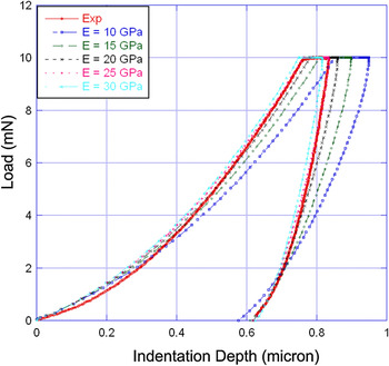
The parameter set P = {E = 25.0 GPa; H = 3.8 GPa; γ = 0.90; β = 20; and η = 3.8 GPa·s} was obtained as satisfactory fit to test data, as shown in Fig. 6. It is necessary, however, to understand how changes in the parameter values affect the load versus indentation depth curve. Figure 6 also shows the effect of changing the parameter E on the nanoindentation creep curve. All other parameters are taken from the set P. As E increases, the slope of the loading and unloading curves increases, as expected.
Effect of changing E (modulus) on the indentation response of bone.

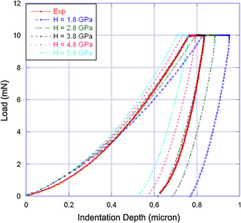
Figure 7 shows the effect of H on the indentation curve. As H increases, one induces a greater “hardening” effect. This hardening effect shifts the curve to the left and does not change the slope of the unloading curve, as expected. Increasing H also decreases the final indentation depth, as expected.
Effect of changing H (slope of linear hardening curve) on the indentation response of bone.

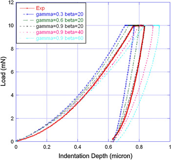
Figure 8 shows the effects of γ and β. As γ and β increase, the slope of the loading curve decreases, and the slope of the unloading curve decreases, with a slight increase in curvature, reproducing the “softening” effect discussed previously.Reference Zhang, Michalenko, Kuhl and Ovaert15
Effect of changing damage parameters γ and β on the indentation response of bone.

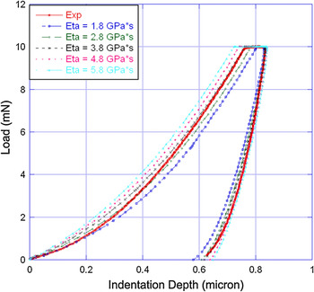
Figure 9 shows the effect of η. As η increases, the creep displacement increases significantly and the slope of the unloading curve increases slightly.
Effect of changing η (viscosity) on the indentation response of bone.

As shown in Figs. 6–9, the parameters in the damage model have very similar effects on the nanoindentation simulation as the corresponding parameter set in the concrete plastic-damage model,Reference Zhang, Michalenko, Kuhl and Ovaert15 however, our UMAT has fewer parameters. This attests to the validity of a damage model for simulating the indentation behavior of bone, and its superiority to the concrete plastic-damage model in terms of its simplicity.
To better understand the simplified indentation model, a more detailed parametric sensitivity study was performed. The sensitivity study can be performed on any number of parameters, thus, we increased the parameters to six by including a change in the yield stress, Y, to determine which parameters have the largest effect on the indentation simulation curve.
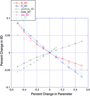
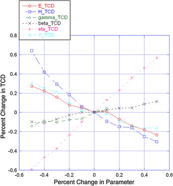
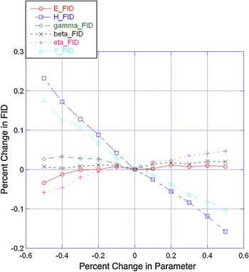
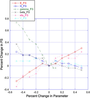
There are various ways to define the characteristics of an indentation curve for a particular interest. A typical option is to look at four key measures: the initial indentation depth (IID) at maximum load, the total creep displacement (TCD) during the holding period, the final indentation depth (FID) at zero load, and the final unloading slope (FS). We examined the parameter sensitivities based on these curve characteristics. The results are shown in Figs. 10–13.
Effect of parameter change on the percent change in initial indentation depth.

Effect of parameter change on the percent change in total creep displacement.

Effect of parameter change on the percent change in final indentation depth.

Effect of parameter change on the percent change in final (unloading) slope.

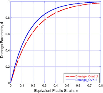
Variation in damage evolution (Eq. 11) for baseline (control) and 2-year postovariectomized ovine bone specimens.

Figure 10 shows the sensitivity of IID to the changes of the six material parameters. It can be seen that IID is almost equally sensitive to all six parameters. Increasing E causes a stiffening response, which will decrease the IID. Increasing H has a similar stiffening effect. Increasing γ increases the limiting value of damage, and a more “damaged” bone decreases the effective stiffness, which will soften the bone and cause the IID to increase. Increasing β increases the amount of damage as well. However, β defines only the damage initiation rate, which has a smaller effect than γ on the amount of damage. Thus, increasing β has a smaller effect than γ on increasing the IID. A larger value of η causes bone to be more viscous. Under the same loading rate (2 mN/s), a more viscous material tends to more strongly resist indenter penetration, which leads to a smaller IID. Increasing Y increases the elastic regime, thus, fewer elements in the finite element mesh have yielded, which causes a stiffening response, thus leading to a smaller IID.
Figure 11 shows the sensitivity of TCD to the material parameters. It can be observed that the TCD is most sensitive to η, as the TCD increases with increasing η. Moreover, the effect of η on TCD is nearly linear. In fact, the creep behavior of bone during the holding period is often solely used to extract the viscoelastic properties of bone. Researchers have used a Burgers model to curve-fit the holding curve during and obtained viscoelastic properties such as the viscosity and time constant.Reference Wu, Baker, Ovaert and Niebur21 The linearity of the effect of η on TCD in the damage model has mathematical benefits, making it easier to determine the viscosity or time constant using the TCD. A second influential parameter on the TCD is H. Decreasing H physically means that the material is increasingly perfectly plastic. Thus, the (decreasing) H curve in Fig. 11 implies that the TCD increases with increased plasticity (decreased H). As viscosity and plasticity both have a large effect on TCD in the damage model, the creep behavior of bone simulated using this model is actually viscoplastic. This feature differentiates our model from the Burgers model, which is purely viscoelastic. The final parameter that influences the TCD to a significant extent is the yield stress, Y. Decreasing Y increases the plastic response and increases the TCD.
Figure 12 shows the sensitivity of the FID to the material parameters. The most influential parameters are the two plasticity-related parameters H and Y. Decreased H represents increased plasticity. A more plastic response results in a deeper FID. The same reasoning applies to Y. The effects of changing the other four parameters on the FID are small. It is noteworthy that for the two damage parameters γ and β, although “damage” and “plasticity” are both irreversible processes, they are different mathematically and physically. In Fig. 12, the fact that changing the amount of damage (γ and β) has little effect on permanent indentation depth also reveals the difference between “damage” and “plasticity” defined in the damage model.
Figure 13 shows the sensitivity of the FS to the material parameters. It can be seen that the effects of the six parameters on FS are all nonlinear, in contrast to the linearity of the previous three figures. However, this does not imply a nonlinearity in the model. In fact, the IID, TCD, and FID are all “length” characteristics, whereas the FS is a characteristic of “force” over “length”. Since “length” is in the denominator, the FS will not be linear. Here, the most influential parameter is the damage parameter γ. As γ increases, the amount of damage increases and FS decreases sharply as shown in Fig. 13. The next influential parameters are E and β. The parameter E, as an elastic parameter, affects the FS as expected. As E increases, the FS increases. The parameter β, as a damage parameter, also affects the FS. However, it has a smaller effect on the FS than γ.
B. Simulation results of baseline and OVX-2 data
As noted above, the damage model contains the parameter set {E, H, Y, η, γ, β}. In multivariate models with more than two or three parameters, it can be very difficult to obtain a unique optimized parameter set, especially when sensitivities to changes in the parameters cause a correspondingly small change in experimental versus simulation curve error. In situations such as these, one can fix the parameters at appropriate values determined experimentally. Thus, in our simulations, E was set as an input value using the average Young’s modulus calculated using the Oliver–Pharr method. Perfect plasticity for bone was assumed,Reference Bayraktar, Morgan, Niebur, Morris, Wong and Keaveny24 thus H = 0. Full damage at the ultimate strain was also assumed, based on previous results,Reference Zhang, Michalenko, Kuhl and Ovaert15 thus γ = 1.0. The results are shown in Table I, with standard deviations shown in parentheses.
Tissue mineral density (TMD), elastic modulus (via Oliver–Pharr), E, Y, η, and β for baseline (control) and 2-year postovariectomized (OVX-2) ovine bone specimens. Standard deviation in parentheses.

The indentation results show that the mean elastic modulus for sample I is greater than that for sample II (using the Oliver–Pharr method). This corresponds to a greater TMD for sample I. The lower TMD value is evidence for osteoporosis in clinical diagnosis of the disease. By fitting the simulation and experimental indentation curves, the yield stress (Y), viscosity (η), and damage initiation rate (β) were also obtained for the samples. The results show that Y for sample I is slightly greater than that for sample II. The value of Y is similar to results in the literature.Reference Burstein, Reilly and Martens25, Reference Hanson, Zioupos, Simpson, Currey and Hynd26
The viscosity, η, for both samples, is similar. The reported values of viscosity for bone differ by orders of magnitude in the literature.Reference Wu, Baker, Ovaert and Niebur21, Reference Lewis and Goldsmith27, Reference Katsamanis and Raftopoulos28 It also appears that the viscosity of bone increases with decreasing strain rate.Reference Zhang, Michalenko, Kuhl and Ovaert15 In a recent study,Reference Wu, Baker, Ovaert and Niebur21 three pure viscoelastic models (standard linear solid, Burgers, and two-dashpot Kelvin) were used in curve fitting to obtain the time constant of bone. It was estimated to be on the order of 1 s. However in this study, the time constant was on the order of 0.1 s, estimated by η / E. The difference in the time constant between the two studies may be due to the different models used. While Wu et al.Reference Wu, Baker, Ovaert and Niebur21 considered the creep period of indentation as a pure viscoelastic process (pure viscoelastic model used), it was considered to be a viscoplastic process in this work, since a viscoplastic damage model was used.
The larger β value for sample II suggests that damage initiates more quickly for OVX-2 bone. Although one may expect the opposite, expecting that bone with a greater TMD would be more brittle (thus more readily damaged via indentation), our results show that damage increases with decreasing TMD, suggesting that osteoporotic bone tends to be less damage-resistant under the same loading conditions. Note that the indentation test serves two purposes here. First, as a method to extract mechanical properties; and second, as a means to induce microdamage. The difference in damage evolution between the two samples can be seen in Fig. 14.
IV. DISCUSSION
As noted above, the viscoelastic-plastic damage model is the simplest material model that contains mechanical properties of elasticity (E), viscoelasticity (η), plasticity (H), and damage (γ and β). For example, plasticity is defined using a linear hardening law and yield stress. Thus, one may wonder if a more precise definition can lead to a better curve-fit result. Under this circumstance, power-law plasticity was then used instead of the linear law to define plasticity in 1D form. Power-law plasticity has the form:
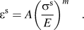
In this case, plasticity is defined using two parameters, A and m, bringing the total number of parameters in the damage model to seven. For a given experimental indentation curve, the damage models using both {E, H, Y, γ, β, η} and {E, A, m, Y, γ, β, η} parameter sets were applied to the simulation. A Matlab optimization program was used to automatically determine the parameters for both cases and to calculate the error between experimental and simulation curves.
The optimization results showed that the difference in the value of the minimized objective function (error between experimental and simulation curves after fit) between the two cases was within 5%. Thus, we could not make a reasonable judgment that one plasticity model was “better” than the other, and it was decided to utilize the linear hardening law since it was simpler from a parameter optimization standpoint.
The scalar damage parameter d, further defined by γ and β, is our selected mathematical definition in this model, which can be seen in Eq. (11). It further quantifies the gradual degradation of the modulus, thus, it affects the stiffness of the material. The scalar damage parameter (d) in the form of Eq. (10) is a widely accepted definition. Thus, the mathematical concept of “damage” in a damage model is different from that in general sense. The permanent indentation depth is mainly a plastic behavior, thus it is not overly sensitive to the changes in γ and β. Additionally, while a decrease in stiffness could markedly increase the permanent indentation depth, previous workReference Zhang, Niebur and Ovaert4 showed that the greatest residual damage was localized to the immediate region beneath the Berkovich tip, while the remaining actual contact area incurs little damage. It is likely that the large “undamaged” area in the contact also acts to inhibit some of the permanent deformation.
Physically, the increased amount of fracture of trabeculae in trabecular bone, and microcracking in cortical bone (which may be viewed as “damage” in a general sense) can lead to both stiffness reduction and increased permanent deformation during indentation. In this sense, fractured trabeculae and microcracks will affect both damage and plasticity parameters in the model.
As a general material model, the viscoelastic-plastic damage model can be used to simulate materials that exhibit quasi-brittle material response. In this sense, Poisson’s ratio (ν) could be included in the parameter set to simulate materials with unknown properties. Thus, the model would then have {E, H, Y, γ, β, η, ν} seven parameters, assuming a linear hardening law.
In the subject of bone mechanical modeling, however, a widely accepted value of 0.3Reference Turner, Rho, Takano, Tsui and Pharr2, Reference Zhang, Niebur and Ovaert4 can be used when treating bone as isotropic, as was the case in this work. Although Poisson’s ratio can vary slightly from sample-to-sample, it is generally not a critical defining parameter. In fact, most contact mechanics simulation results exhibit only a very small sensitivity to changes in the value of Poisson’s ratio, when its value is in the neighborhood of 0.25 to 0.35. If the Poisson’s ratio of bone were extremely high or low values, then it would make more sense to treat it as a viable parameter (i.e., one that could be determined via optimization). Since this is not the case, it was fixed at 0.3.
One limitation of the viscoelastic-plastic damage model is that it ignores the hierarchical structure of bone. The nanostructure of bone starts with tropocollagen molecules that assemble into collagen fibrils in a hydrated environment.Reference Buehler29 The tropocollagen molecules arrange in a quarter-staggered fashion, which leaves periodic gaps between the molecules.Reference Ji and Gao30 Mineralization then occurs within those gaps. The nanometer-sized array of hydroxyapatite crystals is embedded within collagen fibrils. Collagen fibrils range in diameter from 20 to 40 nm.Reference Bartel, Davy and Keaveny31 At the next highest structural level, collagen fibrils arrange in parallel to form a thin sheet called a lamellae, which is several microns thick.
One of the experimental methods used to quantify microdamage in bone is fluorescence microscopy.Reference Zhang, Michalenko, Kuhl and Ovaert15 In the simulations of the baseline and ovariectomized sheep bone nanoindentation data, we used β to quantify damage. This, however, is based on the analysis of the nanoindentation curve. The overall purpose of bone indentation modeling work is to reveal additional mechanical property information (e.g., changes in yield stress, viscosity, damage) from a creep curve, as compared to basic elastic properties and hardness, which is most prevalent in the literature.
Since this damage model is continuum-based, it can only simulate the overall mechanical properties of bone as a continuum material. However, the indentation response of bone actually depends on the properties of the mineral phase, the collagen phase, and the bonding conditions of the two phases. To account for these effects, a multiscale model should be constructed. In addition, establishing the linkage between microdamage obtained from microscopy, to the damage parameters in the damage model, would also be worthwhile. To do this, one must relate microcrack density and distribution, to the degradation of elastic properties on a microscale. Together, these form the basis for future research.
V. CONCLUSIONS
The investigation of bone tissue has always been an important topic due to its relation to human health. Traditional mechanical tests such as torsion and compression provide properties of bone at the macroscale. However, bone microproperties have become increasingly important, and they may be significantly different than their macroscopic counterparts. To obtain the microscopic mechanical properties of bone, nanoindentation is a popular method. To better understand the indentation behavior of bone, numerical modeling and experiments are both necessary.
Viscoelastic-plastic indentation models cannot, in general, be implemented using analytical solutions, especially when plasticity models incorporate linear or nonlinear hardening combined with damage as the basis for explanation of a nonhomogeneous material’s mechanical behavior. This is further complicated when it is desirable to simulate the indenter/substrate geometry and compute stress, strain, and damage fields beneath an actual indenter. Thus, a numerical method (i.e., finite element analysis) is the method of choice when trying to describe complex, but more realistic, bone mechanical behavior. The literature contains an abundance of purely viscoelastic models and applications, however, to the best of our knowledge, viscoelastic-plastic finite element Berkovich indentation models that also incorporate damage parameters are not ubiquitous, and would be the only accurate quantitative choices for a comparison.
In this work, we developed a viscoelastic-plastic damage model for bone indentation simulation, which is the simplest material model that contains mechanical properties of elasticity (E), viscoelasticity (η), plasticity (H), and damage (d). It successfully simulates experimental nanoindentation data from ovine cortical bone.
A sensitivity study was performed to understand the parametric effects in the model. As an improvement to the concrete plastic-damage model used by Zhang et al.,Reference Zhang, Michalenko, Kuhl and Ovaert15 this viscoelastic-plastic damage model has the advantages of generality and simplicity. As a general material model, it may also be used for other materials exhibiting similar quasi-brittle material response.
ACKNOWLEDGMENT
This study was supported by the U.S. National Institutes of Health (ARO52008).