
 MKDN
 MKDN3





1. Introduction
The last two decades have seen the emergence of many offshore wind farms, each of which provides a large amount of green electricity and contribute to a more sustainable future. It is estimated that the whole electricity demand of Europe could be fulfilled with offshore wind farms covering an area of less than one-third of the North Sea (Sørensen & Larsen Reference Sørensen and Larsen2023). To aid such an ambitious development, a theoretical understanding and modelling of wind farm aerodynamics are crucial, but the multiscale nature of the flow makes it a challenging task (Porté-Agel et al. Reference Porté-Agel, Bastankhah and Shamsoddin2020).
The classic approach for modelling wind farm aerodynamics is to model the velocity deficit downstream of each wind turbine, i.e. the ‘wind turbine wake’, with an analytical expression (e.g. Jensen Reference Jensen1983; Bastankhah & Porté-Agel Reference Bastankhah and Porté-Agel2014) and superpose the wakes to obtain the combined wind farm flow (e.g. Katic, Højstrup & Jensen Reference Katic, Højstrup and Jensen1986). Both the wake and superposition models are based on various simplifications to obtain simple analytical forms and do not take into account the response of the atmospheric boundary layer (ABL) to the wind farm. Another classic approach is the ‘top-down models’ (e.g. Frandsen Reference Frandsen1992; Calaf, Meneveau & Meyers Reference Calaf, Meneveau and Meyers2010), which are for very large wind farms, where the flow can be treated as horizontally homogeneous in the interior of the farm and, thus, enables simple modelling of the ABL–wind farm interaction, although without the explicit effect of the turbine layout. A combination of the two above approaches was suggested by Stevens, Gayme & Meneveau (Reference Stevens, Gayme and Meneveau2016), which thereby includes both the effect of turbine layout and the ABL response, but also inherits the empirical assumptions and limitations of the constituent models.
An alternative approach known as the ‘two-scale momentum theory’ was proposed by Nishino & Dunstan (Reference Nishino and Dunstan2020). It is based on the conservation of momentum within the farm region and splits the multiscale flow problem into internal (turbine/array-scale) and external (farm/ABL-scale) subproblems. The internal subproblem is mainly about the turbine–wake interactions, while the external subproblem concerns the farm-scale processes that supply momentum to the farm, and the farm’s interaction with the ABL. By solving the two subproblems together, an estimate for the upper limit of the wind farm performance can be obtained. Furthermore, the power losses in the farm can be classified into turbine-scale (due to wakes impinging downstream turbines) and farm-scale (from the ‘farm-average’ wind speed due to its interaction with the ABL) losses (Kirby, Nishino & Dunstan Reference Kirby, Nishino and Dunstan2022). This classification has later been extended to also include losses due to non-ideal turbine design (Nishino & Smyth Reference Nishino and Smyth2026). Kirby et al. (Reference Kirby, Nishino and Dunstan2022) conducted a suite of 50 large-eddy simulations (LES) of offshore wind farms with varying turbine layouts, which suggested that the farm-scale loss can be more than twice as large as the turbine-scale loss for large wind farms. This has the important implication that there is a limited potential in turbine layout optimisation and that there should be an increased focus on methods that increase wind entrainment into the farm as highlighted by Stevens (Reference Stevens2023).
The two-scale momentum theory has been derived in a general manner, hence, choice of the models for the internal and external subproblems can be varied. In this paper we focus on the external subproblem, which is characterised by the momentum availability factor,
 $M$
, defined as the ratio of momentum transfer into the farm region with and without the turbines present, respectively. The simplest possible model for this quantity is obtained by assuming that there is no interaction between the farm and the ABL, in which case the momentum transfer is equal for the two situations, and therefore,
 $M = 1$
. This simple model was used in the initial study of Nishino (Reference Nishino2016) and by West & Lele (Reference West and Lele2020). More realistically, when the turbines are present, they create a resistance to the ABL, which may enhance the various momentum transport mechanisms (advection, pressure gradient, Coriolis, turbulence and unsteady effects). Hence, it was hypothesised by Nishino & Dunstan (Reference Nishino and Dunstan2020) that the momentum availability should increase approximately linearly as a function of the farm-wind-speed reduction. The proportionality factor of the linear increase of
 $M$
was termed the ‘momentum response factor’ (in later works, it is also called the ‘wind extractability factor’),
 $\zeta$
. Patel, Dunstan & Nishino (Reference Patel, Dunstan and Nishino2021) calculated
 $\zeta$
for a large wind farm in the North Sea using a numerical weather prediction (NWP) simulation and observed it to vary significantly during the day. Using a similar simulation set-up, Kirby et al. (Reference Kirby, Nishino and Dunstan2022) found that
 $\zeta$
is also heavily dependent on the farm size, and later LES confirmed this and showed that it is much less sensitive to the exact turbine layout (Kirby et al. Reference Kirby, Nishino, Lanzilao, Dunstan and Meyers2025).
A more elaborate model of the momentum availability was developed by Kirby, Dunstan & Nishino (Reference Kirby, Dunstan and Nishino2023) through considering each of the momentum transport mechanisms mentioned earlier and modelling each of these independently. By combining the submodels, with some approximations, an analytical model was obtained. A simplified model was also derived from the analytical model using some additional linearisations. Although it was shown that the models appear to perform well, the validity and generality of some underlying assumptions and linearisations could not be confirmed directly at that time as limited LES data was available. In this study we perform an in-depth validation of each contributing mechanism, which is possible with the full three-dimensional (3D) flow fields from the wind farm LES database by Lanzilao & Meyers (Reference Lanzilao and Meyers2024), and with the knowledge obtained from this in-depth validation we propose a new momentum availability model.
An overview of the two-scale momentum theory and the current momentum availability models is given in § 2. The various momentum availability models are then tested against LES data in § 3. In § 4, each momentum availability contribution is evaluated one by one and the validity of the various submodel assumptions are quantified. A new momentum availability model is proposed in § 5, which is based on the ABL Rossby number and can be seen as an extension of the earlier model from Kirby et al. (Reference Kirby, Dunstan and Nishino2023). Finally, conclusions are given in § 6.
2. Theory
2.1. Two-scale momentum theory
The central equation of the two-scale momentum theory (Nishino & Dunstan Reference Nishino and Dunstan2020; Nishino & Smyth Reference Nishino and Smyth2026) is the non-dimensional farm momentum (NDFM) equation
 \begin{equation} C_{\!T}^* \frac {\lambda }{C_{\!f0}} \beta ^2 + \beta ^{\gamma } = M, \end{equation}
where
 $C_T^*$
is the internal farm thrust coefficient,
 $\lambda$
is the array density,
 $C_{\!f0}$
is the surface friction coefficient of the ABL,
 $\beta$
is the wind-speed reduction factor,
 $\gamma$
is the friction exponent and
 $M$
is the momentum availability factor. The exact definitions of these parameters will be given in the summary of the NDFM derivation described below. A typical usage of the equation is to solve for
 $\beta$
, given information or models of the remaining parameters, which can then be used to calculate the farm power efficiency.
The NDFM equation is derived through a control volume (CV) analysis of the streamwise mean momentum equation
 \begin{equation} \frac {\partial \rho U_1}{\partial t} = -\frac {\partial \rho U_1 U_{\!j}}{\partial x_{\!j}} -\frac {\partial\! P}{\partial x_1} + \rho f_c U_2 + \frac {\partial \tau _{1j}}{\partial x_{\!j}} + f_1 \end{equation}
for a volume,
 $V_{{cv}} = \textit{LWH}_{{cv}} = S_{{cv}} H_{{cv}}$
, containing the wind farm. The Reynolds stress tensor is defined as
 $\tau _{ij} \equiv -\rho \overline {u_i u_{\!j}}$
in this work. In the original derivation by Nishino & Dunstan (Reference Nishino and Dunstan2020), the height of the CV was chosen to be similar to the boundary-layer (BL) height,
 $H_{{cv}} \approx \delta _{\textit{ABL}}$
, whereas in later works (e.g. Kirby et al. Reference Kirby, Dunstan and Nishino2023) it has been chosen as
 $H_{{cv}} = H_{\!F}$
(where typically
 $H_{\!F} = 2.5 z_{h}$
is chosen with
 $z_h$
being the turbine hub height, which is also adopted in this work; the sensitivity to
 $H_{\!F}$
is discussed in Appendix A) to model the effects of turbulent entrainment above the wind farm more explicitly than implicitly. For rectangular farm layouts (both aligned and staggered), the length and width of the CV are typically chosen as the number of turbines times inter-spacing, i.e.
 $L = N_x s_x$
and
 $W = N_y s_y$
, where
 $N_i$
and
 $s_i$
are the number of turbines and inter-spacing in the
 $i$
th direction. The NDFM equation will be valid for any choice of CV as long as it encloses the wind farm, but choosing a CV with a size similar to the wind farm is preferred for modelling purposes.
Denoting the volume average over the CV with square brackets (i.e.
 $ [ \boldsymbol{\cdot }] \equiv V_{{cv}}^{-1} \int _{V_{{cv}}} \boldsymbol{\cdot }\text{d}V$
) and using Gauss’s theorem for the advection and turbulent stress terms gives
 \begin{align} \left [\frac { \partial \rho U_1}{\partial t} \right ] &= -\frac {1}{V_{{cv}}}\int _{\varOmega _{{cv}}} \rho U_1 U_{\!j} \text{d}A_{\!j} - \left [ \frac {\partial\! P}{\partial x_1} - \rho f_c U_2 \right ] + \frac {1}{V_{{cv}}} \int _{\varOmega _{{cv}} \setminus \varOmega _w} \tau _{1j} \text{d}A_{\!j} - \frac {S_{{cv}} \tau _w }{V_{{cv}}} - \frac {T}{V_{{cv}}}, \end{align}
where
 $\varOmega _{{cv}}$
is the surface of the CV,
 $\tau _{w} \equiv S_{{cv}}^{-1} \int _{\varOmega _w} \tau _{13} \text{d}A$
is the surface-averaged streamwise component of the wall shear stress (
 $\varOmega _w$
is the wall surface of the CV) and
 $T \equiv - \int _{V_{{cv}}} f_1 \text{d}V$
is the integrated body force stemming from the total turbine thrust forces. Multiplying (2.3) through with the CV and rearranging gives
 \begin{align} T + S_{{cv}} \tau _{w} &= \underbrace {-\int _{\varOmega _{{cv}}} \rho U_1 U_{\!j} \text{d}A_{\!j}}_{X_{{adv}}} \underbrace {- V_{{cv}} \left [ \frac {\partial\! P}{\partial x_1} \right ]}_{X_{\textit{PGF}}} + \underbrace { V_{{cv}} \left [\rho f_c U_2 \right ]}_{X_{\textit{Cor}}} + \underbrace {\int _{\varOmega _{{cv}} \setminus \varOmega _w} \tau _{1j} \text{d}A_{\!j}}_{X_{\textit{turb}}} \underbrace {- V_{{cv}} \left [\frac { \partial \rho U_1}{\partial t} \right ]}_{X_{\textit{uns}}}, \end{align}
where the two terms on the left-hand side are the momentum sinks from the turbine and surface friction drag, respectively, and the terms on the right-hand side are the momentum balancing terms from advection, pressure-gradient forcing, Coriolis, turbulence and unsteadiness. A similar CV analysis can be made for a case without turbines (which has
 $T = 0$
and is denoted with a zero subscript), and this can be used to normalise (2.4), i.e.
 \begin{align} \frac {T + S_{{cv}} \tau _{w}}{S_{{cv}} \tau _{w0}} &= \frac {X_{{adv}} + X_{\textit{PGF}} + X_{\textit{Cor}} + X_{\textit{turb}} + X_{\textit{uns}}}{X_{\textit{adv0}} + X_{\textit{PGF0}} + X_{\textit{Cor0}} + X_{\textit{turb0}} + X_{\textit{uns0}}}. \end{align}
The left-hand side can be rewritten as
 \begin{equation} \frac {T + S_{{cv}} \tau _{w} }{S_{{cv}} \tau _{w0} } = C_{\!T}^* \frac {\lambda }{C_{\!f0}} \beta ^2 + \beta ^{\gamma } \end{equation}
from the definitions
 $C_T^* \equiv T/(({1}/{2}) \rho U_{\!F}^2 N_t A_d)$
,
 $U_{\!F} \equiv [U_1]$
,
 $\lambda \equiv N_t A_d/S_{{cv}}$
,
 $C_{\!f0} \equiv \tau _{w0} / (({1}/{2}) \rho U_{F0}^2)$
,
 $\beta \equiv U_{\!F}/U_{F0}$
and
 $\gamma = \textrm {log}_{\beta } ( {\tau _{w}}/{\tau _{w0}} )$
; hence, (2.5) is, in fact, the NDFM equation (2.1), and the momentum availability factor is
 \begin{equation} M \equiv \frac {X_{\!F}}{X_{\!F0}} = \frac {X_{{adv}} + X_{\textit{PGF}} + X_{\textit{Cor}} + X_{\textit{turb}} + X_{\textit{uns}}}{X_{\textit{adv0}} + X_{\textit{PGF0}} + X_{\textit{Cor0}} + X_{\textit{turb0}} + X_{\textit{uns0}}} . \end{equation}
The contributions of the various physical processes to
 $M$
can conveniently be split into separate parts by rewriting (2.7) as
 \begin{align} M &= 1 + \frac {X_{\!F} - X_{\!F0}}{X_{\!F0}} \\ &= 1 + \underbrace { \frac {X_{{adv}} - X_{\textit{adv0}}}{X_{\!F0}}}_{\Delta M_{{adv}}} + \underbrace { \frac {X_{\textit{PGF}} - X_{\textit{PGF0}}}{X_{\!F0}}}_{\Delta M_{\textit{PGF}}} + \underbrace { \frac {X_{\textit{Cor}} - X_{\textit{Cor0}}}{X_{\!F0}}}_{\Delta M_{\textit{Cor}}} + \underbrace { \frac {X_{\textit{turb}} - X_{\textit{turb0}}}{X_{\!F0}}}_{\Delta M_{\textit{turb}}} + \underbrace { \frac {X_{\textit{uns}} - X_{\textit{uns0}}}{X_{\!F0}}}_{\Delta M_{\textit{uns}}}, \nonumber \end{align}
where one can note that
 $X_{\!F0} = S_{{cv}} \tau _{w0}$
. To solve the NDFM equation, one must model
 $M$
or each individual subpart of it.
2.2. Analytical momentum availability models
The simplest model for
 $M$
is to assume that all
 $\Delta M$
contributions in (2.8) are negligibly small, hence,
 \begin{equation} M_{\textit{constant}} = 1, \end{equation}
which corresponds to assuming that the momentum available to the wind farm is fixed, i.e. there is no ABL response to the farm.
A linear model for
 $M$
was proposed by Nishino & Dunstan (Reference Nishino and Dunstan2020), i.e.
 \begin{equation} M_{\textit{lin}} = 1 + \zeta (1-\beta ), \end{equation}
and further studied by Patel et al. (Reference Patel, Dunstan and Nishino2021) through NWP simulations with a wind farm modelled as an increased surface roughness patch. They concluded that the linear relationship appeared to satisfactorily fit their data with a momentum response parameter
 $\zeta \sim \mathcal{O}(10^1)$
depending on the atmospheric conditions. Using a similar methodology, Kirby et al. (Reference Kirby, Nishino and Dunstan2022) noted that
 $\zeta$
strongly depends on the wind farm size with smaller
 $\zeta$
values being observed for larger wind farms.
A more elaborate model of
 $M$
was developed by Kirby et al. (Reference Kirby, Dunstan and Nishino2023) who considered each term in (2.8) and used various physical arguments to construct submodels of these, which will be discussed in detail in § 4. Their final combined model,
 \begin{equation} M_{\textit{KDN1}} = \frac {1 + \frac {H_{\!F}}{\textit{LC}_{\!f0}} \left ( 1 - \beta ^2 \right ) - \frac { \tau _{t0}}{\tau _{w0}}}{\beta \left (1 -\frac {\tau _{t0}}{\tau _{w0}}\right )}, \end{equation}
was successfully used in conjunction with the NDFM equation to predict the wind farm efficiency for various wind farm LES cases.
Equation (2.11) requires
 $({\tau _{t0}}/{\tau _{w0}})$
, which is often unknown and unavailable as input for prediction of wind farm performance. Kirby et al. (Reference Kirby, Dunstan and Nishino2023) thus suggested to model this ratio as
 $({\tau _{t0}}/{\tau _{w0}}) = 1 - H_{\!F}/h_0$
, which stems from assuming that the (undisturbed) ABL streamwise shear stress is linear from the ground to the ABL height,
 $h_0$
. With this model, one obtains a second simpler version,
 \begin{equation} M_{\textit{KDN}2} = \frac {1 + \frac {h_0}{\textit{LC}_{\!f0}} \left ( 1 - \beta ^2 \right ) }{\beta }, \end{equation}
which, for example, has been used by Nishino & Smyth (Reference Nishino and Smyth2026).
Some further linearisations were given in the appendix of Kirby et al. (Reference Kirby, Dunstan and Nishino2023) to produce a third version, i.e.
 \begin{equation} M_{\textit{KDN}3} = 1 + \underbrace {\left (1.18 + 2.18 \frac {h_0}{\textit{LC}_{\!f0}} \right )}_{\zeta _{\textit{KDN}3}} (1 - \beta ), \end{equation}
which is in a linear form similar to (2.10). The model correctly captures that the momentum response factor,
 $\zeta _{\textit{KDN}3}$
, should decrease with increasing farm size, as discussed earlier, through its dependence on the farm length
 $L$
. Various quasi-one-dimensional (quasi-1D) assumptions were used to obtain (2.11), which is why the farm size is represented by
 $L$
rather than the farm surface area
 $S_{{cv}}$
. A generalisation of
 $M_{\textit{KDN}3}$
to flows with a non-zero inverse ABL Rossby number,
 $\textit{Ro}_{h0}^{-1} \equiv f_c h_0/G$
, named
 $M_{\textit{BNK}}$
, will be developed in § 5.
An overview of the various momentum availability models is given in figure 1, where they are, roughly, categorised according to their accuracy, generality, complexity and the amount of required input. In the next section, these models will be tested using LES data.
Hierarchy of momentum availability models. We propose a new model,
 $M_{\textit{BNK}}$
, in this paper; see § 5. The arrows indicate assumptions to move from one model to another.

3. Validation of momentum availability models with LES data
The momentum availability models presented in the previous section can be tested directly against the true value from LES data. In such a test, the ground truth,
 $M_{\textit{exact}}$
, is obtained by evaluating (2.8) from the time-averaged 3D flow fields in the CV surrounding the wind farm. Hence, full 3D fields of time-averaged velocity, pressure and Reynolds stresses are necessary for such a test.
Contours at hub height of the time-averaged (a–f) streamwise velocity and (g–l) pressure perturbation (subtracted by inlet value). All cases have
 $N_t = 160$
turbines, except the double-spacing and half-farm cases, which have
 $N_t = 40$
and
 $N_t = 80$
, respectively. The inter-spacing is
 $s_x/D = s_y/D = 5$
, except in the double-spacing case. A staggered arrangement is used for all cases, except the aligned case. The farm width (
 $W \equiv N_y s_y$
) is the same for all cases, while the farm length (
 $L \equiv N_x s_x$
) is reduced for the half-farm case. This results in an array density of
 $\lambda = N_t A_d/S_{{cv}} = 0.0314$
for all cases, except the double-spacing case, which has
 $\lambda = 0.00785$
.

Test of existing momentum availability models with LES data.

In this study we consider six cases from the LES database by Lanzilao & Meyers (Reference Lanzilao and Meyers2024). Three cases with the same farm layout but varying ABL heights and three cases with the same ABL height but different wind farm layouts are selected. A precursor-successor methodology was used by Lanzilao & Meyers (Reference Lanzilao and Meyers2024) to simulate the wind farms in conventionally neutral boundary layers (CNBLs). The considered CNBLs are initialised with capping inversion strength
 $\Delta \theta = 5\,{\mathrm{K}}$
and free lapse rate
 $\varGamma = 4\,\mathrm{K\,(km)}^{-1}$
(denoted with suffix ‘C5-G4’ in the database), and three different initial BL heights
 $H=\{300,500,1000\}\,\mathrm{m}$
. A case with
 $H=150\,\mathrm{m}$
also exists in the database, but is not included in the following (see summary of results from this case in Appendix B). All cases have geostrophic velocity
 $G = 10$
m s−1, Coriolis frequency
 $f_c = 1.14 \times 10^{-4}$
s
 $^{-1}$
and aerodynamic roughness length
 $z_0 = 1 \times 10^{-4}$
m. Each wind turbine was modelled as an actuator disk with rotor diameter
 $D = 198$
m, hub height
 $z_h = 119$
m and a uniformly distributed thrust with thrust coefficient
 $C_T'=1.94$
(based on the disk-averaged velocity). After the main simulation had spun up and the flow had reached a quasi-stationary state, the flow statistics were gathered over a time period to obtain first- and second-order statistics of the flow variables throughout the domain. As an example, the time-averaged flow fields at hub height for the six cases are shown in figure 2, from which it is clear that both the ABL height and layout have a large influence on the wind farm flow. For more details about the LES set-up, we refer the reader to Lanzilao & Meyers (Reference Lanzilao and Meyers2024).
Figure 3 shows the test of the various momentum availability models described in the previous section. The highest fidelity model
 $M_{\textit{KDN1}}$
is within
 $\pm 5\,\%$
of
 $M_{\textit{exact}}$
for five of the six cases, but also requires the most input parameters. The simpler
 $M_{\textit{KDN}2}$
and
 $M_{\textit{KDN}3}$
models perform moderately with predictions ranging from
 $-5\,\%$
to
 $25\,\%$
relative to
 $M_{\textit{exact}}$
for four of the six cases, but with a large overprediction for the half-farm and, most severely, for the H1000 case. In general, the
 $M_{\textit{KDN}}$
models appear to decrease in accuracy for increasing ABL heights. The
 $M_{\textit{BNK}}$
model (a new model to be discussed in § 5) does not notably deteriorate in performance for tall ABLs. For completeness, the empirical linear model (2.10) with
 $\zeta = 10$
(the typical order of magnitude; cf. Patel et al. Reference Patel, Dunstan and Nishino2021) and the no-response model ((2.9), i.e.
 $M = 1$
) are also included, but are clearly not performing well and should be avoided. In the next section we quantify the contributions of the various momentum mechanisms to
 $M$
and test the submodels that constitute the
 $M_{\textit{KDN}}$
models.
4. Test of submodels in the
 $M_{\textit{KDN}}$
models

To understand the performance of the
 $M_{\textit{KDN}}$
models, we directly evaluate each constituent part of
 $M$
in this section, i.e. each term in (2.8), from the LES data. It was identified in the previous section that the accuracy of all three versions of the
 $M_{\textit{KDN}}$
model decreases for increasing ABL height, thus, we limit the investigations in this section to the H300, H500 and H1000 cases. The accuracy of the models also decreases for smaller wind farms (see ‘half-farm’ case in figure 3) due to the inherent large-scale wind farm assumptions of the models, but given that offshore wind farms are becoming increasingly larger, we have chosen to not investigate the ‘half-farm’ case further in the current work.
4.1. General observations relevant for the two-scale momentum theory
Some integral quantities of the LES relevant for the two-scale momentum theory are shown in tables 1 and 2. The BL height
 $h_0$
and concavity
 $p_0$
have been estimated through a fit of the normalised total shear stress to
 $|\tau |_0/|\tau |_{w0} = (1 - z/h_0)^{p_0}$
, where
 $|\tau | \equiv \sqrt {\tau _{13}^2 + \tau _{23}^2}$
and the ‘0’ subscript denotes the undisturbed ABL. A discussion about the shape of the ABL shear stress profiles and its relevance for the two-scale momentum theory will be given in § 5. The values of the friction coefficient
 $C_{\!f0}$
are within the typical expected range for offshore wind farms.
Integral quantities for the LES precursor simulations. The quantities are the ABL height
 $h_0$
, concavity of the total shear stress profile
 $p_0$
, normalised mean streamwise velocity in the CV without turbines
 $U_{F0}/G$
, friction coefficient
 $C_{\!f0}$
and the ratio of streamwise shear stress at the top of the CV to streamwise wall shear stress
 $\tau _{t0}/\tau _{w0}$
.

Table 1. Long description
A table comparing integral quantities for LES precursor simulations. The table has four rows and six columns. The column headers are h0 (m), p0, UF0/G, CF0, and τf0/τw0. The row labels are H300, H500, and H1000. Row 1: h0 (m), 360; p0, 1.18; UF0/G, 0.95; CF0, 0.00181; τf0/τw0, 0.099. Row 2: h0 (m), 555; p0, 1.29; UF0/G, 0.94; CF0, 0.00185; τf0/τw0, 0.324. Row 3: h0 (m), 1100; p0, 1.94; UF0/G, 0.92; CF0, 0.00187; τf0/τw0, 0.417.
Integral quantities for the LES wind farm simulations. The quantities are the wind-speed reduction factor
 $\beta$
, the local wind-speed reduction factor at the start of the farm
 $\beta _{\textit{local}}(0)$
, the local wind-speed reduction factor at the end of the farm
 $\beta _{\textit{local}}(L)$
, the friction exponent
 $\gamma$
, the internal thrust coefficient
 $C_T^*$
and the normalised perturbation pressure jump over the farm
 $\Delta P^*/(\rho G^2)$
.

Table 2. Long description
A table comparing integral quantities for wind farm simulations. The table has three rows and seven columns. The columns are labeled Beta, Beta local at start, Beta local at end, Gamma, C T star, and Delta P star over rho G squared. The rows are labeled H 300, H 500, and H 1000. Row 1: Beta, 0.71; Beta local at start, 0.85; Beta local at end, 0.70; Gamma, 1.26; C T star, 1.04; Delta P star over rho G squared, -0.178. Row 2: Beta, 0.74; Beta local at start, 0.88; Beta local at end, 0.74; Gamma, 1.13; C T star, 1.03; Delta P star over rho G squared, -0.180. Row 3: Beta, 0.76; Beta local at start, 0.94; Beta local at end, 0.71; Gamma, 1.05; C T star, 1.03; Delta P star over rho G squared, -0.123.
In earlier studies, it has generally been assumed that the surface friction exponent,
 $\gamma$
, is around 1.7–1.8 (e.g. Kirby et al. Reference Kirby, Nishino and Dunstan2022), but the current LES, see table 2, show that it can be significantly smaller, i.e. around 1.0–1.3. A smaller value of
 $\gamma$
means that the wall friction contribution, i.e.
 $\beta ^\gamma = \tau _w/\tau _{w0}$
, in the NDFM equation (2.1), becomes larger (because
 $0 \lt \beta \lt 1$
). Nevertheless, as shown in figure 4, the farm thrust term, i.e.
 $C_{\!T}^*({\lambda }/{C_{\!f0}}) \beta ^2 = T/(S_{{cv}} \tau _{w0})$
, is still the dominant momentum sink on the left-hand side of the NDFM equation for all cases. This is an important observation because it implies that the modelling of
 $\gamma$
is not critical to the prediction of
 $\beta$
. One can therefore, in many cases, assume that
 $\gamma = 2$
to simplify the NDFM equation without incurring any significant error, even if the true value of
 $\gamma$
is closer to one. On the other hand, the modelling of the internal thrust coefficient,
 $C_T^*$
, is more important for obtaining good predictions of
 $\beta$
with the NDFM equation. Regarding
 $C_T^*$
, table 2 shows that it is nearly constant for all three simulations, which is consistent with the fundamental two-scale assumption in the sense that it is mainly an ‘internal’ parameter of the wind farm (i.e. depends mainly on turbine layout and turbine operating conditions) and, therefore, is not expected to be sensitive to the ABL height, which is an ‘external’ parameter (Kirby et al. Reference Kirby, Nishino, Lanzilao, Dunstan and Meyers2025). The modelling of
 $C_T^*$
was investigated by Kirby et al. (Reference Kirby, Nishino and Dunstan2022) and Nishino & Smyth (Reference Nishino and Smyth2026) and will not be further discussed in this paper.

The development of the local wind-speed reduction factor
 $\beta _{\textit{local}} \equiv (H_{\!F} {\textit{WU}}_{F0})^{-1} \int _0^{H_{\!F}} \int _0^{\textit{W}} \,U_{1}\text{d}y \,\text{d}z$
and the perturbation pressure
 $P^* \equiv P - P_\infty$
(where
 $P_\infty$
is the background pressure, which is linearly decreasing in the horizontal direction according to the driving pressure gradient force (PGF),
 $\partial\! P_\infty /\partial x_i$
, of the simulation) are shown in figure 5. The small ‘high-frequency’ fluctuations in the farm region are from the individual turbines, whereas the larger fluctuations, which are also present in farm wakes (Lanzilao & Meyers Reference Lanzilao and Meyers2025), are from farm-induced gravity waves. Gravity waves are also clearly visible in figure 2 and have been studied in detail by Lanzilao & Meyers (Reference Lanzilao and Meyers2024) among others. They are generally stronger for lower ABL heights and it is also seen in figure 5(b) that a lower ABL height induces a larger pressure perturbation drop,
 $\Delta P^*$
, over the farm region, which is favourable for farm power production. The pressure perturbation,
 $P^*$
, should go to the same constant value,
 $P_{\textit{inlet}}^*$
, far upstream and downstream of the farm, but it does not despite the fact that a large domain was used for the LES, which suggests that an even longer domain should ideally have been used. An error can be expected from this in the PGF term of the momentum availability factor, but this is not expected to change the main conclusions of the following analysis.
(a) Local wind-speed reduction factor, and (b) normalised perturbation pressure (subtracted by inlet value) spanwise averaged over the width
 $y=[y_{\textit{centre}}-W/2,y_{\textit{centre}}+W/2]$
and height
 $z=[0,H_{\!F}]$
of the CV. The CV region enclosing the wind farm is marked in grey.

(a) Contributions from CV surfaces to the advection term for LES (full) and the model (dashed). A positive sign means advection of
 $U_1$
into the CV. Note that the north and south contributions are almost identical. (b) Total advection contribution and error of the model.

4.2. Advection
Streamwise momentum is advected in and out of the CV, and its contribution,
 $\Delta M_{{adv}}$
, to the momentum availability factor is defined in (2.8). For our current cases, the expression for the advection part simplifies to
 \begin{align} \Delta M_{{adv}} &= \frac {X_{{adv}}}{X_{\!F0}} = \frac {-\int _{\varOmega _{{cv}}} \rho U_1 U_{\!j} \text{d}A_{\!j}}{X_{\!F0}}, \end{align}
because
 $X_{\textit{adv}0} = 0$
due to the horizontal homogeneity of the precursor simulations (the front/rear and north/south advection cancel due to periodicity and the top/bottom advection are zero because
 $U_3 = 0$
). There is also no flow through the bottom surface in the main simulation, hence, only the front/rear, north/south and top surfaces of the CV contribute to the integral, which are calculated directly from the LES flow field data and displayed in figure 6(a). In the advection submodel of Kirby et al. (Reference Kirby, Dunstan and Nishino2023) it was assumed that the north/south contributions were zero, but as shown in figure 6(a), both of these are in fact negative for the current cases (meaning there is advection out of the CV at these surfaces) due to the flow through the farm diverting horizontally spanwise. However, in comparison with the other contributions, the north/south contributions are indeed small and it is therefore a reasonable approximation to neglect them. The front/rear contributions used in their submodel are exact, as they can be rewritten as
 \begin{equation} - \frac {1}{X_{\!F0}} \int _{\varOmega _{\textit{front}}} \rho U_1 U_{\!j} \text{d}A_{\!j} = \frac {2 \beta _{\textit{local}}(0)^2 H_{\!F}}{\textit{LC}_{\!f0}}, \end{equation}
 \begin{equation} - \frac {1}{X_{\!F0}} \int _{\varOmega _{\textit{rear}}} \rho U_1 U_{\!j} \text{d}A_{\!j} = - \frac {2 \beta _{\textit{local}}(L)^2 H_{\!F} }{\textit{LC}_{\!f0}} . \end{equation}
The sign change on the former is because the vectors
 $U_{\!j}$
and
 $\text{d}A_{\!j}$
have opposite directions on the front face. Finally, for the top surface Kirby et al. (Reference Kirby, Dunstan and Nishino2023) used a simple quasi-1D mass flux analysis to estimate its contribution as
 \begin{align} - \frac {1}{X_{\!F0}} \int _{\varOmega _{\textit{top}}} \rho U_1 U_{\!j} \text{d}A_{\!j} &= \frac {H_{\!F} \left ( \beta _{\textit{local}}(L)^2 - \beta _{\textit{local}}(0)^2 \right )}{\textit{LC}_{\!f0}} . \end{align}
In all cases,
 $\beta _{\textit{local}}(L) \lt \beta _{\textit{local}}(0)$
, hence, the model always predicts advection out of the top surface (i.e. a negative contribution). The LES data in figure 6(a) however show that there is advection into the CV (i.e. a positive contribution) for the lowest ABL height case, H300, which can occur due to the strong gravity waves present in this case. The model for the top surface advection (4.4) overpredicts the advection out of the top surface in all cases, which in effect compensates for the neglected advection out of the north/south surfaces. The overall advection submodel of Kirby et al. (Reference Kirby, Dunstan and Nishino2023) is the sum of (4.2)–(4.4), i.e.
 \begin{equation} \Delta M_{{adv}} = \frac { H_{\!F}}{\textit{LC}_{\!f0}} \big ( \beta _{\textit{local}}(0)^2 - \beta _{\textit{local}}(L)^2 \big), \end{equation}
and figure 6(b) shows it is within approximately
 $\pm 10\,\%$
of the LES data. As it depends on
 $\beta _{\textit{local}}(0)$
and
 $\beta _{\textit{local}}(L)$
, which are in general unknown, it is by itself not a very practical analytical model and it will therefore be further simplified in § 4.4.
4.3. Pressure gradient forcing
The CNBLs used in the current cases are driven by a horizontal pressure gradient forcing,
 $(\partial\! P_\infty /\partial x_1,\partial\! P_\infty /\partial x_2)$
, which is constant throughout the domain, i.e. it is a barotropic ABL, and, as shown in figure 5(b), a perturbation PGF,
 $\partial\! P^*/\partial x_1$
, develops in the CV region due to the presence of the wind farm (recall that
 $P^* \equiv P - P_\infty$
is defined as the pressure perturbation from the linearly decreasing background pressure
 $P_\infty$
that drives the flow). The contribution from the pressure gradient to the momentum availability is defined in (2.8) and the expression for the PGF part can be rewritten with the perturbation pressure as
 \begin{align} \Delta M_{\textit{PGF}} &= -\frac {V_{{cv}}}{X_{\!F0}} \left [ \frac {\partial\! P^*}{\partial x_1}\right ] = - \frac {H_{\!F}}{L \tau _{w0}} \underbrace {\left ( P_{\textit{rear}}^* - P_{\textit{front}}^* \right )}_{\equiv \Delta P^*}, \end{align}
where
 $P_{\textit{rear}}^*$
and
 $P_{\textit{front}}^*$
are the rear and front surface-averaged values, respectively. Equation (4.6) is exact and was the starting point for Kirby et al. (Reference Kirby, Dunstan and Nishino2023), who used Bernoulli’s equation to estimate the front perturbation pressure as
 \begin{equation} P_{\textit{front}}^* - P_{\textit{inlet}}^* = \frac {1}{2} \rho U_{F0}^2 \big ( 1 - \beta _{\textit{local}}(0)^2\big ), \end{equation}
where
 $P_{\textit{inlet}}^*$
is the far upstream value. The second assumption of their PGF model is that the rear perturbation pressure is simply the negative value of the above, i.e.
 \begin{equation} P_{\textit{rear}}^* - P_{\textit{inlet}}^* = -\big(P_{\textit{front}}^* - P_{\textit{inlet}}^* \big), \end{equation}
which corresponds to assuming that
 $P^* - P_{\textit{inlet}}^*$
is anti-symmetric around the centre of the farm. Combining (4.8) with (4.6) and (4.7) gives the final submodel of Kirby et al. (Reference Kirby, Dunstan and Nishino2023):
 \begin{equation} \Delta M_{\textit{PGF}} = 2 \frac {H_{\!F}}{\textit{LC}_{\!f0}} \big (1 - \beta _{\textit{local}}(0)^2 \big ). \end{equation}
(a) Contributions from the front and rear surfaces to the PGF term for LES (full) and the model (dashed). (b) Total PGF contribution and error of the model.

The two assumptions, i.e. (4.7) and (4.8), are checked with the LES data in figure 7(a), which shows that the simple Bernoulli estimate fairly well captures the trend of the front pressure, whereas the rear assumption is less consistent. Regarding the latter, it can indeed be observed in figure 5(b) that the perturbation pressure is not perfectly anti-symmetric around the centre of the farm. The H500 case is closest to being anti-symmetric, which is consistent with the fact that this is the case with the best rear prediction. As discussed at the end of § 4.1, the LES domain length is possibly too short to simulate the pressure field around the farm accurately, although it is not clear how large the impact of the LES domain length is and if a longer inlet fetch would improve the agreement between the LES and model.
The difference between the two dashed lines (or full lines) in figure 7(a) is the pressure perturbation jump,
 $\Delta P^*$
, over the farm, which per (4.6) determines the PGF contribution to
 $M$
. It can be seen that the pressure jump is overestimated by the model for the H300 and H500 cases, which is why
 $\Delta M_{\textit{PGF}}$
is overestimated for these two cases; see figure 7(b). Nevertheless, the model correctly captures that the PGF contribution tends to decrease with increasing ABL height, which is expected because the ABL top acts as a ‘lid’ on the flow and thereby affects the pressure gradient within the farm (a taller ABL height gives a smaller enhancement of the favourable wind farm pressure gradient). The effect of the ABL height on the wind farm pressure field has also been studied in detail by Lanzilao & Meyers (Reference Lanzilao and Meyers2024).
(a) Test of the advection pressure (AP) approximation (red lines) and the underlying assumption (i) (4.13) (blue lines). (b) Combination of the advection and PGF terms of the momentum availability factor. The error percentage indicated is between the model and AP approximation bars.

4.4. The AP approximation
Combining the advection and PGF models ((4.5) and (4.9)) gives
 \begin{align} \Delta M_{{adv}} + \Delta M_{\textit{PGF}} &= \frac {H_{\!F}}{\textit{LC}_{\!f0}} \big ( - \beta _{\textit{local}}(0)^2 - \beta _{\textit{local}}(L)^2 + 2 \big ), \end{align}
which can be simplified to
 \begin{align} \Delta M_{\textrm {adv}} + \Delta M_{\textrm {PGF}} &= \frac {H_{\!F}}{\textit{LC}_{\!f0}} \big ( 1 - \beta ^2 \big ), \end{align}
resulting from the ‘AP approximation’,
 \begin{equation} \beta _{\textit{local}}(0)^2 + \beta _{\textit{local}}(L)^2 \approx 1 + \beta ^2 . \end{equation}
This approximation was proposed by Kirby et al. (Reference Kirby, Dunstan and Nishino2023) by assuming that the decrease of
 $\beta _{\textit{local}}$
from upstream (where it has a value of 1) to the front of the farm is equal to the increase from the farm-averaged value (i.e.
 $\beta$
) to
 $\beta _{\textit{local}}$
at the end of the farm, i.e.
 \begin{equation} 1 - \beta _{\textit{local}}(0) \approx \beta _{\textit{local}}(L) - \beta, \quad \textrm {assumption (i)}, \end{equation}
which when squared and rearranged becomes
 \begin{align} 1 + \beta ^2 &\approx \beta _{\textit{local}}(L)^2 + \beta _{\textit{local}}(0)^2 + 2 \left ( \beta _{\textit{local}}(L) \beta _{\textit{local}}(0) - \beta \right ) . \end{align}
This equation simplifies to (4.12) when the second assumption is invoked:
 \begin{align} 2 \left ( \beta _{\textit{local}}(L) \beta _{\textit{local}}(0) - \beta \right ) \approx 0, \quad \textrm {assumption (ii)} . \end{align}
The data from the LES in figure 8(a) show an absolute error of around 0.1–0.2 for assumption (i) (4.13). The error from this first assumption means that (4.14) is not exactly correct, which together with the error from the second assumption leads to the fact that the AP approximation gives an overestimation of
 $\beta _{\textit{local}}(L)^2 + \beta _{\textit{local}}(0)^2$
by around 10–25 %. In contrast, Kirby et al. (Reference Kirby, Dunstan and Nishino2023) only found an overprediction of around 10 % for the four LES cases they analysed. The overprediction of the AP approximation means that the sum of the advection and PGF terms gets underpredicted by 30–35 %, see figure 8(b), because
 $\beta _{\textit{local}}(0)^2 + \beta _{\textit{local}}(L)^2$
appears with a negative sign in (4.10). These results highlight the difficulty in accurately predicting the advection and PGF terms without using the local flow information (such as
 $\beta _{\textit{local}}$
) as input.
4.5. Coriolis
It was assumed by Kirby et al. (Reference Kirby, Dunstan and Nishino2023) that the contribution from the Coriolis force to the momentum availability factor could be neglected, i.e.
 \begin{equation} \Delta M_{\textit{Cor}} = 0 . \end{equation}
To verify the correctness of this, we evaluate its contribution directly from the LES data using its definition (2.8), which is
 \begin{align} \Delta M_{\textit{Cor}} &= \frac {V_{{cv}} \rho f_c}{X_{\!F0}} \left ( \left [U_2\right ] - \left [U_2\right ]_0\right ) = \frac {2 }{C_{\!f0} \textit{Ro}_{F0}} \left ( \frac {\left [U_2\right ] - \left [U_2\right ]_0 }{U_{F0}}\right ) \!, \end{align}
where
 $\textit{Ro}_{F0} \equiv U_{F0}/(f_c H_{\!F})$
is a Rossby number based on the CV height and no-turbine farm velocity. All three simulations have
 $ {2 }/({C_{\!f0} \textit{Ro}_{F0}}) \approx 4$
(which can be evaluated from the values in table 1), but the change of CV-averaged spanwise velocity from the precursor to main simulation is small,
 $ (( { [U_2 ] - [U_2 ]_0 )}/{U_{F0}} ) = \mathcal{O}(0.01)$
, and therefore
 $\Delta M_{\textit{Cor}}$
is only around
 $0.05$
, see table 3. This is much smaller than the contributions from the advection, PGF and turbulence terms, and the Coriolis term in the momentum equation thus contributes to less than
 $1 \,\%$
of the total
 $M$
. It is therefore a good assumption to neglect the direct Coriolis contribution. However, as shown in § 5, the Coriolis effect still has an important indirect influence on the momentum availability through shear stress veering, which cannot be neglected.
The LES and model predictions of the Coriolis contribution.

Table 3. Long description
A table comparing Coriolis contribution predictions across different simulations. The table has four columns and three rows. The columns are labeled as follows: 2/Cf0RoF0, [Uz]−[U2]0/Uf0, ΔMCor (LES), ΔMCor (model), and ΔMCor/M [%](LES). The rows are labeled as H300, H500, and H1000. Row 1: 2/Cf0RoF0, 3.94; [Uz]−[U2]0/Uf0, 0.02; ΔMCor (LES), 0.08; ΔMCor (model), 0.00; ΔMCor/M [%](LES), 0.8. Row 2: 2/Cf0RoF0, 3.93; [Uz]−[U2]0/Uf0, 0.01; ΔMCor (LES), 0.06; ΔMCor (model), 0.00; ΔMCor/M [%](LES), 0.5. Row 3: 2/Cf0RoF0, 3.97; [Uz]−[U2]0/Uf0, 0.01; ΔMCor (LES), 0.04; ΔMCor (model), 0.00; ΔMCor/M [%](LES), 0.4.
4.6. Unsteadiness
The effect of (farm-scale) unsteadiness on the momentum availability was assumed to be negligible in the model of Kirby et al. (Reference Kirby, Dunstan and Nishino2023), i.e.
 \begin{align} \Delta M_{\textit{uns}} = 0. \end{align}
To validate this, the time history of the flow is necessary, which is not available in the LES database of Lanzilao & Meyers (Reference Lanzilao and Meyers2024). As an alternative, we instead consider the time-averaged and horizontally averaged streamwise momentum budgets to implicitly give an assessment of the stationarity of the flow in the present LES.
The momentum budget for a CNBL precursor simulation is given by
 \begin{align} \left \langle \frac {\partial U_1}{\partial t}\right \rangle = \left \langle - \frac {1}{\rho } \frac {\partial\! P_\infty }{\partial x_1}\right \rangle + \left \langle f_c U_2\right \rangle + \left \langle \frac {1}{\rho } \frac {\partial {\tau _{13}}}{\partial x_3}\right \rangle \!, \end{align}
where
 $\langle \boldsymbol{\cdot }\rangle$
is the horizontal-average operator. The advection term is zero and the stress divergence term is simplified due to the periodic boundary conditions applied in the horizontal directions. A subscript
 $\infty$
is used on the pressure to denote that this is the driving pressure of the ABL. The budgets of the three considered ABLs are shown in figure 9 together with the sum of the terms on the right-hand side of (4.19). In the interior of the ABLs, the sum has a small positive value (meaning that
 $U$
is increasing in time), but it is nevertheless significantly smaller than the other terms, and we thus conclude that the ABLs are close to being stationary (i.e. ‘quasi-stationary’). Previous studies of the CNBL have indicated that around six non-dimensional time units are sufficient for the flow to reach a quasi-stationary state (Pedersen, Gryning & Kelly Reference Pedersen, Gryning and Kelly2014; Liu et al. Reference Liu, Gadde and Stevens2021a
, Reference Liu, Lu and Stevens2024) and Lanzilao & Meyers (Reference Lanzilao and Meyers2024) indeed time-averaged the flow over the non-dimensional time period
 $f_c t = [8.6, 9.2 ]$
.
Momentum budget for CNBL precursor simulations. The grey area marks the CV region.

The momentum budget for a wind farm simulation is given by
 \begin{align} \left \langle \frac {\partial U_1}{\partial t}\right \rangle = \left \langle - \frac {\partial U_1 U_{\!j} }{\partial x_{\!j}}\right \rangle + \left \langle -\frac {1}{\rho } \frac {\partial\! P^* }{\partial x_1}\right \rangle + \left \langle -\frac {1}{\rho } \frac {\partial\! P_\infty }{\partial x_1}\right \rangle + \left \langle f_c U_2\right \rangle + \left \langle \frac {1}{\rho }\frac {\partial \tau _{1j}}{\partial x_{\!j}}\right \rangle + \left \langle \frac {1}{\rho } f_1\right \rangle \!, \end{align}
where the horizontal-average operator
 $\langle \boldsymbol{\cdot }\rangle$
is over the CV surface area,
 $S_{{cv}}$
, only. No body force fields are available in the analysed LES dataset, but the body force term in (4.20) can nevertheless still be obtained, because the total farm thrust,
 $T$
, is known, and because the thrust on each actuator disk is distributed uniformly; hence, similar to the actuator wind farm (AWF) model (van der Laan et al. Reference van der Laan, Baungaard, Meyer Forsting and Réthoré2024), we find that the force is distributed in the vertical direction as
 \begin{equation} q_{{ver}}(z) = \begin{cases} \frac {4}{\pi D} \sqrt {1 - ([z-z_H]/R)^2} &\quad \textrm {if} \quad |(z-z_H)/R| \leqslant 1, \\[7pt] 0 &\quad \textrm {if} \quad |(z - z_H)/R| \gt 1, \\ \end{cases} \end{equation}
and thus, we have
 \begin{align} \left \langle \frac {1}{\rho }f_1\right \rangle = q_{{ver}}\frac {T}{S_{{cv}} \rho } . \end{align}
Figure 10 shows the budgets for the three cases and again the sum of the terms is close to zero at all heights, thus signifying quasi-stationarity of the wind farm flows as well. In summary, we conclude that the transient evolution of the streamwise momentum is small in the present LES and that the contribution of unsteadiness to the momentum availability can be neglected for all three cases.
Momentum budget for wind farm simulations. The grey area marks the CV region.

4.7. BL height
Kirby et al. (Reference Kirby, Dunstan and Nishino2023)’s submodel of the momentum availability contribution from turbulence, to be discussed in § 4.8, depends on the height of the undisturbed ABL
 $h_0 \equiv \delta (x=-\infty )$
and the farm BL
 $h \equiv L^{-1} \int _{x_{wf,\textit{start}}}^{x_{wf,\textit{start}}+L} \delta (x) \,\text{d}x$
. There are several ways to define the BL height,
 $\delta (x)$
, and in this section we define it as the height at which the shear stress,
 $\tau _{13}$
, is equal to 5 % of its ABL surface value
 $\tau _{w0}$
(e.g. Kosović & Curry Reference Kosović and Curry2000). Figure 11 shows the spanwise-averaged streamwise shear stress from the three cases and highlights the contour line corresponding to the BL height. A large shear stress region develops in and above the wind farm in all cases due to the large velocity gradient,
 $\partial U / \partial z$
, induced by the turbines, and this region eventually reaches the capping inversion layer and pushes it upwards until the buoyant destruction from the stable stratification of the free atmosphere is sufficiently large to suppress the turbulence. It is this complex balance that dictates the spatial evolution of
 $\delta (x)$
.
Contours of the spanwise-averaged (over the CV width
 $y=[y_{\textit{centre}}-W/2,y_{\textit{centre}}+W/2]$
) streamwise shear stress. The line styles used denote the BL height
 $\delta (x)$
from LES (
 ) and the model (
 ). The farm region is highlighted with a grey box and the model error,
 $(h^{\textit{model}} - h^{\textit{LES}})/h^{\textit{LES}}$
, is shown.

Kirby et al. (Reference Kirby, Dunstan and Nishino2023) proposed a simple model for the spatial development of the BL height from a quasi-1D continuity analysis
 \begin{equation} \delta (x) = \frac {h_0}{\beta _{\textit{local}}(x)}, \end{equation}
which is shown with dashed lines in figure 11. It can be seen that the model correctly captures an increase of the BL height in the farm region, but that it is less accurate for taller ABLs. In the H1000 case, the BL height first starts to increase after approximately a half farm length, which is in line with the fact that the shear stress region develops at an angle (not directly upwards from the wind farm entrance) and that, for taller ABLs, it thus takes a longer streamwise distance to reach the ABL height. The inability of the model to capture this is due to its quasi-1D assumption and that the model is derived from mass continuity, which implicitly implies that the BL height is directly related to the velocity field, i.e. that
 $\delta (x)$
follows the ‘separating’ streamline between the ABL and the free atmosphere, rather than the shear stress field.
To obtain a model for the farm BL height,
 $h$
, Kirby et al. (Reference Kirby, Dunstan and Nishino2023) used (4.23) in the definition of
 $h$
described in the beginning of the current subsection to obtain
 \begin{equation} h = \frac {1}{L} \int _{x_{wf,\textit{start}}}^{x_{wf,\textit{start}}+L} \delta (x) \text{d}x = \frac {h_0}{L} \int _{x_{wf,\textit{start}}}^{x_{wf,\textit{start}}+L} \frac {1}{\beta _{\textit{local}}} \text{d}x \approx \frac {h_0}{\beta }, \end{equation}
and assumed that the last integral is equal to
 $L/\beta$
, which thereby gives their final BL height displacement model
 \begin{equation} \frac {h_0}{h} = \beta . \end{equation}
The ‘integral assumption’, i.e. the last equality in (4.24), was confirmed by Kirby et al. (Reference Kirby, Dunstan and Nishino2023) with four LES cases from Wu & Porté-Agel (Reference Wu and Porté-Agel2017) to be very good (within 0.5 % of the actual value) and we find the same for the cases studied in this paper. This means that the error of
 $h^{\textit{model}}$
compared with
 $h^{\textit{LES}}$
, which, as shown in figure 11, is of the order of 7–17 %, is almost entirely from (4.23). This overprediction of
 $h$
has a significant influence on the model prediction of
 $\Delta M_{\textit{turb}}$
, which we will return to in the next section.
4.8. Turbulence
The last contributing term to the momentum availability factor is from turbulence,
 $\Delta M_{\textit{turb}}$
, which entrains mean momentum into the wind farm through enhanced mixing. It is defined in (2.8) and it should be noted that it does not include the wall shear stress. Writing out its terms gives
 \begin{align} \Delta M_{\textit{turb}} &= \frac { X_{\textit{turb}} - X_{\textit{turb}0}}{X_{\!F0}} = \frac { \int _{\varOmega _{{cv}}\setminus \varOmega _w} \tau _{1j} \text{d}A_{\!j} - \int _{\varOmega _{\textit{top}}} \tau _{1j,0} \text{d}A_{\!j} }{X_{\!F0}}, \end{align}
where only the top surface contribution from the precursor case is present, because the front/rear and south/north terms cancel in the precursor due to horizontal homogeneity. Equation (4.26) is exact, but to obtain a practical model, Kirby et al. (Reference Kirby, Dunstan and Nishino2023) proceeded without the front/rear and south/north contributions from the farm case. As shown in figure 12, this is a good assumption, except for the rear contribution, which is negative (it entrains momentum out of the CV) with a magnitude of around 10 % of the top surface entrainment (which is positive and entrains momentum into the CV). If one nevertheless neglects the rear contribution, the equation simplifies to
 \begin{equation} \Delta M_{\textit{turb}} = \frac {\tau _t - \tau _{t0} }{\tau _{w0}}, \end{equation}
where we have dropped the subscript ‘13’ and denote the surface-averaged shear stress on the CV top surface as
 $\tau _{t} \equiv S_{{cv}}^{-1} \int _{\varOmega _{\textit{top}}} \tau _{13} \text{d}A$
and used the fact that
 $X_{\!F0} = \tau _{w0} S_{{cv}}$
.
Contributions to
 $\Delta M_{\textit{turb}}$
evaluated from LES data at the various surfaces of the CV.

To model
 $\tau _t$
, Kirby et al. (Reference Kirby, Dunstan and Nishino2023) assumed that the streamwise shear stress profiles of the ABL and farm simulations, see figure 13(a), are self-similar above the top-tip height, i.e.
 \begin{equation} \frac {\tau _0\left (z/h_0\right )}{\tau _{w0}} = \frac {\tau (z/h)}{\tau _{w1}} \quad (\mathrm{for}\,z \gt z_{\textit{hub}} + D/2), \end{equation}
where a second (fictive) wall shear stress is defined as
 $\tau _{w1} \equiv M \tau _{w0}$
. One can interpret
 $\tau _{w1}$
as the wall shear stress one would obtain by extrapolating the
 $\tau (z)$
profile above the top-tip height of the turbines to the ground. Figure 13(b) shows that all profiles do not exactly collapse to a single curve, but that each pair of ABL/farm simulations does, which is the important part because this justifies the use of (4.28).
Streamwise shear stress profiles of the precursor ( ) and farm region of the wind farm simulation (
 ) (a) and test of their self-similarity (b). The fictive wall shear stress
 $\tau _{w1} \equiv M \tau _{w0}$
is directly obtained through LES data of
 $M$
and
 $\tau _{w0}$
. The ABL and farm heights are defined with the 5 % (of
 $\tau _{w0}$
and
 $\tau _{w1}$
, respectively) rule.

Equation (4.28) can be rearranged to
 \begin{align} \tau (z) = \tau _{w1}\frac {\tau _0\left (z \frac {h_0}{h}\right )}{\tau _{w0}}, \end{align}
which is used to obtain the top shear stress
 \begin{align} \tau _t = \tau _{w1}\frac {\tau _0\left (H_{\!F} \frac {h_0}{h}\right )}{\tau _{w0}} . \end{align}
To use this expression one needs
 $\tau _0 (H_{\!F} {h_0}/{h} )$
, which Kirby et al. (Reference Kirby, Dunstan and Nishino2023) obtained by assuming a linear profile of
 $\tau _0(z)$
in the interval
 $z= [0,H_{\!F} ]$
, i.e.
 \begin{align} \tau _0(z) = \tau _{w0} + \frac {\tau _{t0} - \tau _{w0}}{H_{\!F}} z \quad \quad (\mathrm{for}\, 0 \lt z \lt H_{\!F}), \end{align}
leading to
 $\tau _0 (H_{\!F} {h_0}/{h} ) = \tau _{w0} + (\tau _{t0} - \tau _{w0}) ({h_0}/{h})$
. Inserting this expression into (4.30) gives
 \begin{align} \tau _t &= M \left (\tau _{w0} + (\tau _{t0} - \tau _{w0}) \frac {h_0}{h} \right ) \!, \end{align}
which combined with (4.27) results in Kirby et al. (Reference Kirby, Dunstan and Nishino2023)’s submodel for the turbulence contribution to the momentum availability:
 \begin{align} \Delta M_{\textit{turb}} = M + M\left (\frac {\tau _{t0}}{\tau _{w0}} - 1\right ) \frac {h_0}{h} - \frac { \tau _{t0}}{\tau _{w0}} . \end{align}
Unlike the other submodels, this expression is implicit (
 $\Delta M_{\textit{turb}}$
is inside
 $M$
on the right-hand side), but, due to its simple form, inserting (4.33) into (2.8) with the other submodels nevertheless leads to an explicit relation for
 $M$
:
 \begin{equation} M = \frac {1 + \frac {H_{\!F}}{\textit{LC}_{\!f0}} \left ( 1 - \beta ^2 \right ) - \frac { \tau _{t0}}{\tau _{w0}}}{ \left (1 -\frac {\tau _{t0}}{\tau _{w0}}\right ) \frac {h_0}{h}} . \end{equation}
This expression is equal to the first version of the KDN model,
 $ M_{\textit{KDN1}}$
(2.11), when the BL height model
 $h_0/h = \beta$
(4.25) is used.
(a) The BL height ratio
 $h_0/h$
from LES (
 $h$
based on 5 % of
 $\tau _{w1}$
, c.f. figure 13) and the model of
 $h_0/h = \beta$
(4.25). The LES value of
 $h/h_0$
with
 $h$
based on 5 % of
 $\tau _{w0}$
, c.f. figure 11, is also displayed, although it is not the relevant height ratio for the
 $\Delta M_{\textit{turb}}$
model. (b) Model of turbulence contribution to the momentum availability and its error.

To test the
 $\Delta M_{\textit{turb}}$
submodel, as shown in figure 14(b), one first evaluates
 $M$
from (4.34) and subsequently inserts this into (4.33). Hence, the turbulence contribution indirectly depends on the other submodels and the BL height ratio
 $h_0/h$
through (4.34). It should be emphasised that the dependence on the farm BL height
 $h$
originates from the self-similarity assumption (4.28), which as shown in figure 13(b) is based on the height where the streamwise shear stress is equal to 5 % of
 $\tau _{w1}$
. It thus differs from the farm BL height displayed in figure 11, which was based on 5 % of
 $\tau _{w0}$
, and this explains why, counter-intuitively,
 $h_0/h$
can exceed one, e.g. the H1000 case in figure 14(a). As discussed in the previous section, the BL height ratio model (4.25) overpredicts
 $h/h_0$
(based on
 $\tau _{w0}$
) by 7–17 % corresponding to an underprediction of
 $h_0/h$
of about the same amount. However, when comparing the model with
 $h_0/h$
based on
 $\tau _{w1}$
, the underprediction is larger, 19–36 %, which is the main reason for the large overprediction of
 $\Delta M_{\textit{turb}}$
shown in figure 14(b). Other sources of errors are from the no rear-entrainment, linear shear stress profile across the CV height and self-similarity assumptions, but these are found to be secondary. We find that
 $\Delta M_{\textit{turb}}$
is also overpredicted for shallow ABLs (see Appendix B) and the ‘half-farm’ case, which underlines that this term is the most complex term of (2.8) to model.
4.9. Summary of the momentum availability contributions
The findings from the previous sections are summarised in figure 15. Each bar has the same total value as the corresponding one from figure 3(a–c), but the current figure reveals the split between the various momentum contributions to
 $M$
. From this, we conclude that
 $\Delta M_{{adv}}$
,
 $\Delta M_{\textit{PGF}}$
and
 $\Delta M_{\textit{turb}}$
are approximately equally important and that none of these can be neglected. For the
 $M_{\textit{KDN1}}$
model, the advection and PGF contributions are grouped together due to the AP approximation (4.11). The model correctly captures the fact that the turbulence contribution increases with increasing ABL height (this is because the shear stress at the top of the CV increases), although the magnitude is overpredicted as discussed in the previous subsection. Nevertheless, the turbulence overprediction is consistently compensated by the underprediction of the AP approximation, hence, the final model prediction of
 $M_{\textit{KDN1}}$
is within
 $\pm 1$
% of
 $M_{\textit{exact}}$
, which is excellent considering the complexity of the momentum availability. Despite the good total performance of
 $M_{\textit{KDN1}}$
, its practical applicability is limited, since it is nonlinear in
 $\beta$
and a priori requires a value of
 $\tau _{t0}/\tau _{w0}$
, which is the motivation for the
 $M_{\textit{KDN}2}$
and
 $M_{\textit{KDN}3}$
models.
Split of the momentum availability for the LES data (full) and the
 $M_{\textit{KDN1}}$
model (crossed).

4.10. The
$M_{\textit{KDN}2}$
and
$M_{\textit{KDN}3}$
models


The
 $M_{\textit{KDN}2}$
and
 $M_{\textit{KDN}3}$
models are derived from the
 $M_{\textit{KDN1}}$
model as shown in the overview in figure 1. The
 $M_{\textit{KDN}2}$
model is first derived by assuming a linear shear stress profile, which is then further simplified to
 $M_{\textit{KDN}3}$
by two linearisations for the relationship between
 $M$
and
 $\beta$
, but the order in which these simplifications are applied is arbitrary and results in the same linear model,
 $M_{\textit{KDN}3}$
. We have selected the current order of simplifications, because the nonlinear
 $M_{\textit{KDN}2}$
model is a practical model on its own, as, for example, used by Nishino & Smyth (Reference Nishino and Smyth2026).
The assumption required to simplify
 $M_{\textit{KDN1}}$
(2.11) to
 $M_{\textit{KDN}2}$
(2.12) is that
 $\tau _0(z)$
is linear from
 $z=0$
to
 $z=h_0$
, which gives
 \begin{equation} 1 -\frac {\tau _{t0}}{\tau _{w0}} \approx \frac { H_{\!F}}{h_0}. \end{equation}
This assumption is more restrictive compared with (4.31), where
 $\tau _0(z)$
was only assumed to be linear up to
 $z=H_{\!F}$
. Also,
 $h_0$
in this context refers not to the 5 % height but to the full ABL height, i.e. where the streamwise shear stress goes to zero. In the ABL literature (e.g. Berg, Patton & Sullivan Reference Berg, Patton and Sullivan2020; Liu et al. Reference Liu, Gadde and Stevens2021b
),
 $h_0$
is usually defined from the total shear stress
 $|\tau |_0 = \sqrt {\tau _{13,0}^2 + \tau _{23,0}^2}$
, which is preferred due to its frame invariance and because it better represents the actual ABL height, and we therefore choose to use this height as
 $h_0$
(obtained from LES by fitting
 $|\tau |_0/|\tau |_{w0} = (1 - z/h_0)^{p_0}$
; see table 1) in the evaluation of the
 $M_{\textit{KDN}2}$
model and in the rest of the paper. As already presented in figure 3, the LES data show that the
 $M_{\textit{KDN}2}$
model is significantly less accurate than the
 $M_{\textit{KDN1}}$
model, especially for taller ABLs, and we propose a model extension to amend this in § 5.
The
 $M_{\textit{KDN}2}$
model (2.12) can be rearranged to
 \begin{align} M_{\textit{KDN}2} &= \frac {1}{1 - (1 - \beta )} + \frac { \frac {h_0}{\textit{LC}_{\!f0}} \left ( 2\left ( 1 - \beta \right ) - (1 - \beta )^2 \right ) }{1 - (1 - \beta )}, \end{align}
and simplified to
 $M_{\textit{KDN}3}$
(2.13) using the linearisations suggested by Kirby et al. (Reference Kirby, Dunstan and Nishino2023):
 \begin{equation} \frac {1}{1 - (1 - \beta )} \approx 1 + 1.18 (1 - \beta ), \quad \textrm {linearisation (i)}, \end{equation}
 \begin{equation} \frac { 2\left ( 1 - \beta \right ) - (1 - \beta )^2 }{1 - (1 - \beta )} \approx 2.18 (1 - \beta ), \quad \textrm {linearisation (ii)}. \end{equation}
Figure 16 shows the results of applying these two linearisations. Linearisation (i) is applied to the first term in (4.36), which is approximately one order of magnitude smaller than the second term, hence, this linearisation has little impact on the solution. Adding the second linearisation has a larger effect, which, actually, improves the prediction of
 $M$
slightly, making it closer to
 $M_{\textit{KDN1}}$
. Overall, both linearisations, however, have a relatively small effect, compared with the linear shear stress assumption (4.35) used for simplifying
 $M_{\textit{KDN1}}$
to
 $M_{\textit{KDN}2}$
, and therefore, we focus on modifying this assumption in the next section.


5. The ABL Rossby number extension of
$\boldsymbol{M_{\textit{KDN}3}}$

The
 $M_{\textit{KDN}3}$
model (2.13) is easy to use in practical applications as it only requires the ABL height
 $h_0$
, farm length
 $L$
and friction coefficient
 $C_{\!f0}$
, but as shown in figure 3, and in the previous section, it significantly overpredicts
 $M$
for wind farms operating in tall ABLs. In this section we derive a new momentum availability model
 $M_{\textit{BNK}}$
, see figure 1, by including a dependence on the ABL Rossby number
 $\textit{Ro}_{h0} \equiv G/(f_c h_0)$
. The new model reduces to
 $M_{\textit{KDN}3}$
for the special case of
 $\textit{Ro}_{h0}^{-1} = 0$
and can thus also be viewed as an extension of this model.
It was identified in the previous section that the principal error of the
 $M_{\textit{KDN}3}$
model stems from the assumption that
 \begin{equation} 1 -\frac {\tau _{xt0}}{\tau _{xw0}} \approx \frac { H_{\!F}}{{h}_0}, \end{equation}
which comes from assuming a linear profile,
 $\tau _{x0}(z)/\tau _{xw0} = 1 - z/h_0$
and evaluating it at
 $z =H_{\!F}$
to obtain
 $\tau _{xt0} = \tau _{x0}(H_{\!F})$
. Note that a more explicit notation is used in (5.1) and the rest of this section, i.e. a subscript
 $x$
is added to the stresses to denote the direction, compared with in the previous sections (where the subscript
 $x$
was omitted for brevity); table 4 gives a summary of the variables and notation used in the following analysis. The problem with (5.1) is that
 $h_0$
is the ABL height defined based on the total shear stress, which is typically larger than the ABL height defined based on the streamwise shear stress,
 $h_{x0}$
. Secondly, the streamwise shear stress profile is not linear, but slightly concave, which implies that an even smaller height,
 $\tilde {h}_{x0} \lt h_{x0}$
, should be used as sketched in figure 17. We thus propose to replace (5.1) with
 \begin{equation} 1 -\frac {\tau _{xt0}}{\tau _{xw0}} \approx \frac { H_{\!F}}{\tilde {h}_{x0}}, \end{equation}
corresponding to assuming a hypothetical linear profile
 $\tilde {\tau }_{x0}(z)/\tau _{xw0} = 1 - z/\tilde {h}_{x0}$
that gives
 $\tilde {\tau }_{x0}(H_{\!F}) = \tau _{xt0}$
. To use (5.2), a model for
 $\tilde {h}_{x0}$
is needed.
Summary of shear stress and BL height definitions for the undisturbed ABL used in § 5.

Table 4. Long description
The table lists symbols, names, and formulas related to shear stress and BL height definitions. It includes various symbols such as tau subscript r0(z), tau subscript rw0, and tau subscript r10, each with corresponding names and formulas. The formulas involve variables like u1, u2, u3, z, and hx0, and operations such as multiplication, division, and exponentiation. The table provides a structured overview of the relationships and calculations involved in defining shear stress and BL height in the undisturbed atmospheric boundary layer.
Sketch of ABL profiles of total shear stress
 $|\tau |_0(z)$
, streamwise shear stress
 $\tau _{x0}(z)$
and a hypothetical stress
 $\tilde {\tau }_{x0}(z)$
, which is linear and gives
 $\tilde {\tau }_{x0}(H_{\!F}) = \tau _{x0}(H_{\!F}) = \tau _{xt0}$
.

Power function fits of the (a) total and (b) streamwise shear stress ABL profiles.

If the streamwise shear stress profile can be expressed as a power function, i.e.
 \begin{equation} \frac {\tau _{x0}(z)}{\tau _{xw0}} = \left (1 - \frac {z}{h_{x0}}\right )^{p_{x0}}\!, \end{equation}
it is simple mathematical problem to determine
 $\tilde {h}_{x0}$
from
 $(H_{\!F},h_{x0},p_{x0})$
. Evaluating (5.3) at
 $z = H_{\!F}$
to obtain
 $\tau _{xt0}/\tau _{xw0}$
and inserting this into (5.2) yields
 \begin{align} \frac {\tilde {h}_{x0}}{H_{\!F}} = \left (1 - \left (1 - \frac {H_{\!F}}{h_{x0}} \right )^{p_{x0}}\right )^{-1} \!. \end{align}
This expression can, with good accuracy, be linearised to
 \begin{align} \frac {\tilde {h}_{x0}}{H_{\!F}} \approx 1 + p_{x0}^{-1.25} \left ( \frac {h_{x0}}{H_{\!F}} - 1 \right )\!, \end{align}
for relevant values of
 $p_{x0}$
and
 $h_{x0}/H_{\!F}$
(for
 $1 \lt p_{x0} \lt 2$
and
 $1 \lt h_{x0}/H_{\!F} \lt 5$
, the error is around
 $\pm 3\,\%$
).
Figure 18 shows power function fits to the three ABL profiles of
 $|\tau |_0(z)$
and
 $\tau _{x0}(z)$
. Nieuwstadt (Reference Nieuwstadt1984) suggested an exponent of
 $p_0 = 3/2$
for the total shear stress in the stable ABL, which in later works has also been used for the CNBL (e.g. Liu et al. Reference Liu, Gadde and Stevens2021b
; Kirby et al. Reference Kirby, Dunstan and Nishino2023; Baungaard et al. Reference Baungaard, van der Laan, Kelly and Hodgson2024), but the fits in figure 18(a) show that this does not seem to be a universal value for the CNBL. Instead, it appears that the shear stress profile becomes more concave for taller ABLs. Secondly, it is observed that
 $h_{x0} \lt h_0$
and
 $p_{x0} \gt p_0$
with the difference stemming from the veering of the shear stress vector caused by the Coriolis effect (in the special case of no Coriolis,
 $f_c=0$
, they would be identical). Thus, even though it was found in § 4.5 that the Coriolis force itself does not contribute significantly to the momentum availability, i.e.
 $\Delta M_{\textit{Cor}} \approx 0$
, the Coriolis effect does have an indirect influence on
 $M$
through
 $\Delta M_{\textit{turb}}$
from shear stress veering.
The fitted values of
 $h_{x0}/h_0$
and
 $p_{x0}$
are plotted against the inverse ABL Rossby number,
 $\textit{Ro}_{h0}^{-1}$
, in figure 19 along with fits from other CNBL LES from the literature (all data were rotated to align the hub-height wind direction with the
 $x$
axis before fitting; this implicitly makes the hub height a parameter in the model). Despite some scatter of the data, which can be expected due to different numerics, case set-up, integration time and strong dependence on the temperature initialisation (e.g. Allaerts & Meyers Reference Allaerts and Meyers2017), some trends of
 $h_{x0}/h_0$
and
 $p_{x0}$
as a function of
 $\textit{Ro}_{h0}^{-1}$
can be observed. The Heck & Howland (Reference Heck and Howland2025) data appears to have an opposing trend for
 $p_{x0}$
, but nevertheless scatter approximately equally around the trend line. It has also been found by van der Laan et al. (Reference van der Laan, Kelly, Floors and Peña2020) that a Rossby number related to the ABL height (they use a turbulence length scale,
 $\ell _{\textit{max}}$
, which correlates with the ABL height) is a central parameter for capped ABLs. In the limit of zero Coriolis,
 $\textit{Ro}_{h0}^{-1} = 0$
, the data are seen to asymptote towards
 $h_{x0}/h_0 = 1$
and
 $p_{x0} = 1$
as expected.
To analytically predict
 $h_{x0}/h_0$
and
 $p_{x0}$
, we fit super-Gaussian and linear functions, respectively, to the LES data that satisfy the asymptotic behaviour of
 $h_{x0}/h_0$
and
 $p_{x0}$
for
 $\textit{Ro}_{h0}^{-1} = 0$
as
 \begin{align} \frac {h_{x0}}{h_0} = \textrm {exp}\left ( - \left (\frac {\textit{Ro}_{h0}^{-1}}{0.02}\right )^3 \right )\!, \\[-12pt]\nonumber\end{align}
 \begin{align} p_{x0} = 1 + 70 \textit{Ro}_{h0}^{-1}, \end{align}
which are plotted together with the data in figure 19.
Fitted parameters from power function fits in figure 18. Additional data from other CNBL LES (Berg et al. Reference Berg, Patton and Sullivan2020; Baungaard et al. Reference Baungaard, van der Laan, Kelly and Hodgson2024; Liu, Lu & Stevens Reference Liu, Lu and Stevens2024; Heck & Howland Reference Heck and Howland2025) are also included.

To summarise, the new proposed model is
 \begin{equation} M_{\textit{BNK}} = 1 + \underbrace {\left (1.18 + 2.18 \frac {\tilde {h}_{x0}}{\textit{LC}_{\!f0}} \right )}_{\zeta _{\textit{BNK}}} (1 - \beta ), \end{equation}
with
 \begin{equation} \tilde {h}_{x0} = H_{\!F} + \left (1 + 70 \textit{Ro}_{h0}^{-1}\right )^{-1.25} \left ( h_{0} \, \textrm {exp}\left ( - \left (\frac {\textit{Ro}_{h0}^{-1}}{0.02}\right )^3 \right ) - H_{\!F} \right ) \!. \end{equation}
Note that this new model has two additional input parameters,
 $\textit{Ro}_{h0}$
and
 $H_{\!F}$
, compared with the
 $M_{\textit{KDN}3}$
model (2.13), but is still posed in a similar linear form for practicality. For the special case of
 $\textit{Ro}_{h0}^{-1} = 0$
, we obtain
 $\tilde {h}_{x0} = h_0$
from (5.9) and the new model is then identical to the
 $M_{\textit{KDN}3}$
model. The explicit dependence on
 $H_{\!F}$
(which is not present in the
 $M_{\textit{KDN}3}$
model) is physically consistent, because
 $M$
is independent of
 $H_{\!F}$
, whereas
 $\beta$
is dependent on
 $H_{\!F}$
, hence,
 $\zeta$
should be dependent on
 $H_{\!F}$
. The sensitivity on
 $H_{\!F}$
is further discussed in Appendix A.
To test the new model, we first compare the momentum response factor
 \begin{equation} \zeta \equiv \frac {M - 1}{1 - \beta }, \end{equation}
which highlights the principal difference between the proposed
 $M_{\textit{BNK}}$
model and the
 $M_{\textit{KDN}3}$
model from Kirby et al. (Reference Kirby, Dunstan and Nishino2023) (this quantity is only defined for linear models, which is why it was not shown in the comparison in § 3). Figure 20 shows the comparison, where it is most notable that the new model corrects the previously heavily overpredicted
 $\zeta$
for the H1000 case. Overall, the new model improves the prediction of
 $\zeta$
for five out of the six cases.


As a second test, we solve the NDFM equation (2.1), which, for linear momentum availability models, can be rewritten as
 \begin{equation} \left (C_{\!T}^* \frac {\lambda }{C_{\!f0}} + 1\right ) \beta ^2 = 1 + \zeta (1 - \beta ), \end{equation}
where we have further assumed that
 $\gamma = 2$
(the actual
 $\gamma$
values are given in table 2) to simplify the left-hand side. This latter assumption only introduces a small error because the first term in (2.1) is dominating as shown earlier in figure 4, and turns the equation into a quadratic polynomial, which can be solved analytically for
 $\beta$
(the positive root). With the value of
 $\beta$
obtained, one can finally predict the global wind farm power efficiency,
 \begin{equation} C_{\!PG} \equiv \frac {\sum _{i=1}^{N_t} P_i}{\frac {1}{2} \rho N_t A_d U_{F0}^3} = \beta ^3 C_{\!P}^*, \end{equation}
where
 $C_{\!P}^* = ({\sum\nolimits_{i=1}^{N_t} P_i})/({({1}/{2}) \rho N_t A_d U_{F}^3})$
is the internal wind farm power coefficient. Figure 21 shows the comparison of
 $C_{\!PG}$
, where an improved prediction is also observed for five out of the six cases with the new model. Again, the most significant improvement is for the tall ABL case, H1000, which indeed also is the case with the largest
 $\textit{Ro}_{h0}^{-1}$
value and, thus, is most affected by the new Rossby sensitisation.
Model parameters and momentum response factor compared with staggered wind farm LES.

Table 5. Long description
The table compares model parameters and momentum response factors for different wind farm configurations. It has three columns and ten rows, including headers. The columns are labeled with different configurations: Wu & Port-Agel (2017) with 36 times 5 turbines, Wu & Port-Agel (2017) with 20 times 9 turbines, and Allaerts & Meyers (2017) with 20 times 9 turbines. The rows list various parameters and their values for each configuration. Row 1: h 0, 410, 656, 1102. Row 2: R e h 0 superscript negative 1, 0.0049, 0.0078, 0.0092. Row 3: C f 0, 0.0061, 0.0054, 0.0016. Row 4: L, 20.2, 20.2, 15.0. Row 5: H F slash z h, 2.5, 2.5, 2.5. Row 6: beta LES, 0.82, 0.79, 0.80. Row 7: M LES, 2.19, 2.89, 11.50. Row 8: zeta LES minus zeta i n f, 6.5, 9.0, 52.2. Row 9: zeta K D N 3 minus zeta LES, 28.9, 58.6, 94.4. Row 10: zeta LES minus zeta B N K, 8.1, 8.7, 16.2.


Finally, we consider some ‘out-of-sample’ wind farm cases from Wu & Porté-Agel (Reference Wu and Porté-Agel2017) and Allaerts & Meyers (Reference Allaerts and Meyers2017). As in Kirby et al. (Reference Kirby, Dunstan and Nishino2023), we take the hub-height wind speed normalised by the inflow value as a proxy of
 $\beta _{\textit{local}}(x)$
to calculate
 $\beta = L^{-1} \int _0^L \beta _{\textit{local}}(x) \text{d}x$
. The spanwise-averaged total shear stress profile in the centre of the farm is extrapolated to the ground to obtain the fictive
 $\tau _{w1}$
, which can be used to obtain a proxy of the momentum availability as
 $M = \tau _{w1}/\tau _{w0}$
(see figure 13). It is thus possible to estimate the momentum response factor
 $\zeta _{\textit{LES}}$
for these LES (despite the fact that the full 3D flow data are not available), which is compared with
 $\zeta _{\textit{KDN}3}$
and
 $\zeta _{\textit{BNK}}$
in table 5. As in the Lanzilao & Meyers (Reference Lanzilao and Meyers2024) cases, the error of the KDN3 model is larger for taller ABLs (or larger
 $\textit{Ro}_{h0}^{-1}$
) and results are consistently improved with the Rossby number extension. However, there is still an overprediction of
 $\zeta _{\textit{BNK}}$
of 8–16 % compared with
 $\zeta _{\textit{LES}}$
, but in this regard it should be noted that there is likely a significant uncertainty on the latter due to the proxy methods used to obtain
 $M_{\textit{LES}}$
and
 $\beta _{\textit{LES}}$
. Nevertheless, the results still clearly indicate that the new model offers a robust improvement over the KDN3 model from Kirby et al. (Reference Kirby, Dunstan and Nishino2023) with minimal addition of model complexity.
6. Conclusion
The thrust from wind turbines and the ground (or sea-surface) friction drag are resistances to the atmospheric flow through a wind farm region, and these momentum sinks are balanced by a collection of momentum fluxes from various mechanisms (advection, pressure gradient, Coriolis, turbulence and unsteadiness), which together are called the momentum availability. The momentum availability is a key parameter in the two-scale momentum theory of wind farm flows (Nishino & Dunstan Reference Nishino and Dunstan2020), which is a theoretical modelling framework for predicting wind farm efficiency based on separating turbine/array- and farm/ABL-scales. In this study, we have validated the analytical momentum availability model from Kirby et al. (Reference Kirby, Dunstan and Nishino2023) using a LES dataset of wind farm simulations by Lanzilao & Meyers (Reference Lanzilao and Meyers2024) and proposed a new practical extension to improve its generality/accuracy.
There are three versions of Kirby et al. (Reference Kirby, Dunstan and Nishino2023)’s analytical momentum availability model, which we label
 $M_{\textit{KDN1}}$
,
 $M_{\textit{KDN}2}$
and
 $M_{\textit{KDN}3}$
in order of their fidelity/complexity, and test against LES data from six wind farm cases. The six cases consist of three with the same turbine layout but different ABL heights, and three with the same ABL height but different turbine layouts. In comparison with
 $M_{\textit{exact}}$
, the exact value from the LES data, the
 $M_{\textit{KDN1}}$
model has an error between
 $-3$
% to 1 % for five out of the six cases (there is a larger error of
 $22$
% for the half-farm case due to its smaller size, where the inherent large-scale assumption of the model is less valid), which is good given the complexity of the momentum availability. The more practical
 $M_{\textit{KDN}2}$
and
 $M_{\textit{KDN}3}$
models, which are simpler and require fewer input parameters, on the other hand, only agree well with
 $M_{\textit{exact}}$
for the lowest ABL case and have significantly larger errors with up to around 100 % overprediction for the tallest ABL case. In general, we observe that the accuracy of all three versions decreases with increasing ABL heights, and we thus focus on the three LES cases with different ABL heights in the majority of the paper. Offshore wind farms are becoming increasingly large, which explains our motivation for mainly focusing on the different ABL height cases rather than the smaller half-farm case in this work.
To understand the validity of the underlying assumptions of the
 $M_{\textit{KDN}}$
models, each individual contribution to the momentum availability is evaluated from the LES data, which reveals that the advection, pressure gradient and turbulence terms are the main contributors and of similar magnitude, whereas the contributions from the Coriolis force and unsteadiness can safely be neglected. Although, the direct Coriolis contribution is negligible, there is nevertheless still an indirect influence of the Coriolis effect, due to shear stress veering, which cannot be neglected. The advection submodel of Kirby et al. (Reference Kirby, Dunstan and Nishino2023) is found to generally perform well with only small errors coming from the neglected advection out of the lateral sides of the farm and the modelled advection out through the top of the farm. There is a larger error for the pressure gradient submodel, especially for the case with a low ABL height (H300), but the model nevertheless correctly captures that its contribution decreases with increasing ABL height. This phenomenon can be attributed to the induced favourable pressure gradient through the farm region, which gets stronger as the ABL height is decreased (Lanzilao & Meyers Reference Lanzilao and Meyers2024). The turbulence submodel requires the most modelling and it is found to be especially sensitive to the modelling of the farm BL height. Overall, however, the submodels consistently compensate the errors of each other leading to the good overall performance of the
 $M_{\textit{KDN1}}$
model for the comprehensive dataset of Lanzilao & Meyers (Reference Lanzilao and Meyers2024) representing future large offshore wind farms. Whether this compensation of errors has a physical basis is currently unknown to us and could be a topic for future research. Finally, it is also identified from the LES data that the assumption of a linear shear stress profile in the ABL is the root cause of the degradation of accuracy in the
 $M_{\textit{KDN}2}$
model, whereas the two linearisations to obtain
 $M_{\textit{KDN}3}$
are fairly accurate.
A comparison of ABL shear stress profiles from a range of different CNBL studies (Berg et al. Reference Berg, Patton and Sullivan2020; Baungaard et al. Reference Baungaard, van der Laan, Kelly and Hodgson2024; Liu et al. Reference Liu, Lu and Stevens2024; Lanzilao & Meyers Reference Lanzilao and Meyers2024; Heck & Howland Reference Heck and Howland2025) shows that the concavity
 $p_0$
and
 $p_{x0}$
, and ABL height
 $h_0$
and
 $h_{x0}$
, of the total and streamwise shear stress profiles, respectively, vary considerably. Trends of
 $h_{x0}/h_0$
and
 $p_{x0}$
as a function of the inverse ABL Rossby number
 $\textit{Ro}_{h0}^{-1} = f_c h_0/G$
can be identified, for which some simple theoretical models are proposed. Using these models, a nonlinear streamwise stress profile can be predicted analytically, which is the basis for our new momentum availability model
 $M_{\textit{BNK}}$
. This model reduces to
 $M_{\textit{KDN}3}$
for the special case of
 $\textit{Ro}_{h0}^{-1} = 0$
(thus, one can also view it as an extension of
 $M_{\textit{KDN}3}$
) and is similarly in a linear form, which makes the model simple and practical to use in wind farm power prediction. The
 $M_{\textit{BNK}}$
model amends the issues with the
 $M_{\textit{KDN}3}$
model for tall ABL cases. In particular, the error of the two-scale momentum theory prediction of global wind farm power efficiency is reduced from 42 % to 4 % for the case with the tallest ABL height (H1000), while still retaining, or even further improving, its prediction also for lower ABL heights. The
 $M_{\textit{BNK}}$
model depends on the Coriolis frequency
 $f_c$
through
 $\textit{Ro}_{h0}^{-1}$
and it is thus expected to be more generally applicable compared with the
 $M_{\textit{KDN}3}$
model, while still remaining in a simple linear form, which justifies its position in the hierarchy of momentum availability models in figure 1. Its development is based on CNBLs, so its validity in other types of ABLs is not clear, which may limit its application range and could be a topic for future studies. The application of the current model for shallow ABLs with smaller ABL height than the turbine top-tip height may be limited (see Appendix B) and would be an important topic for further investigations due to the trend of larger wind turbines. Another interesting future subject is the modelling of momentum availability for wind farm wakes, which is increasingly becoming more important due to the ever growing number of offshore wind farms.
Acknowledgements
M.B. acknowledges the Carlsberg Foundation for his funding, Linacre College for his fellowship and the Department of Engineering Science at the University of Oxford for hosting him. We thank Luca Lanzilao and Johan Meyers for open sourcing the data from their wind farm LES, which have been instrumental for this paper. We also thank Kirby Heck, Luoqin Liu and their co-authors for sharing relevant CNBL LES data.
Funding
This research has been partly supported by the Carlsberg Foundation (grant no. CF-1002) and the UK Natural Environment Research Council (NERC ECOFlow programme, NE/Z504099/1).
Declaration of interests
The authors report no conflict of interest.
Data availability statement
The LES data that support the findings of this study are openly available in the KU Leuven RDR database at https://doi.org/10.48804/L45LTT, (Lanzilao & Meyers Reference Lanzilao and Meyers2024). Post-processed data and plotting scripts are available at https://github.com/mchba/Validation-and-extension-of-an-analytic-momentum-availability-model.
Author contributions
M.B. post-processed the LES data and produced the figures. T.N. supervised the research. M.B. proposed the ABL Rossby number extension, which builds upon the analytical momentum availability model originally proposed by A.K and T.N. M.B. wrote the paper with corrections from T.N. and A.K.
Appendix A. Sensitivity of momentum response factor to CV height
The momentum availability
 $M$
is independent of the choice of CV height
 $H_{\!F}$
, which follows from the NDFM equation (2.1), because the left-hand side is equal to
 $(T+S_{{cv}} \tau _w)/(\tau _{w0} S_{{cv}})$
(see (2.6)), where
 $T$
,
 $\tau _{w}$
,
 $\tau _{w0}$
and
 $S_{{cv}}$
are all independent of
 $H_{\!F}$
. The wind-speed reduction factor
 $\beta$
, on the other hand, is dependent on
 $H_{\!F}$
. This follows directly from its definition,
 $\beta \equiv U_{\!F}/U_{F0}$
, where both
 $U_{\!F}$
and
 $U_{F0}$
depend on
 $H_{\!F}$
, but in different ways (except for the trivial case, where the turbines are shut off). Combining these observations, one can conclude that the momentum response factor
 $\zeta \equiv (M-1)/(1 - \beta )$
(defined in (5.10)) must be dependent on
 $H_{\!F}$
.
Both the
 $M_{\textit{KDN}3}$
model (2.13) and the proposed
 $M_{\textit{BNK}}$
model (5.8) are of the form
 $M = 1 + \zeta (1 - \beta )$
, but only the latter has a dependence on
 $H_{\!F}$
in its model of
 $\zeta$
(as physically required following the discussion above). To visualise the effect of
 $H_{\!F}$
,
 $\zeta$
has been computed from the LES data of the H300, H500 and H1000 cases with a range of different choices of
 $H_{\!F}$
and compared with the prediction of the two models in figure 22. The LES results show that
 $\zeta$
increases slightly for increasing
 $H_{\!F}$
and a similar behaviour can be seen for the new model due to its explicit dependence on
 $H_{\!F}$
, whereas the KDN3 model predicts constant
 $\zeta$
. As such, the new model is more robust to the choice of
 $H_{\!F}$
, although its value in practice is typically chosen as
 $H_{\!F}/z_h = 2.5$
(Kirby et al. Reference Kirby, Nishino and Dunstan2022, Reference Kirby, Dunstan and Nishino2023).
Momentum response factor sensitivity to CV height. The LES values are calculated as
 $\zeta _{\textit{LES}} = (M_{\textit{LES}} - 1)/(1 - \beta _{\textit{LES}})$
, while
 $\zeta _{\textit{KDN}3}$
and
 $\zeta _{\textit{BNK}}$
are calculated with (2.13) and (5.8), respectively. Nishino & Dunstan (Reference Nishino and Dunstan2020) suggested choosing
 $H_{\!F}$
from the condition
 $ {(\int _0^{H_{\!F}} U_0 dz)}/{H_{\!F}} = {(\int U_0 \text{d}A)}/{A}$
, which for all three cases gives
 $H_{\!F}/z_h \approx 2.3$
, but
 $H_{\!F}/z_h = 2.5$
was nevertheless chosen for the current work following Kirby et al. (Reference Kirby, Nishino and Dunstan2022, Reference Kirby, Dunstan and Nishino2023). The error of the models at this
 $H_{\!F}$
is displayed, which corresponds to the errors in figure 20(a–c).

Appendix B. Results of the shallow ABL ‘H150’ case
The dataset of Lanzilao & Meyers (Reference Lanzilao and Meyers2024) also includes a case with initial BL height
 $H=150\,\mathrm{m}$
, which could have been included in the main text, but was nevertheless omitted because the physics in such a shallow ABL regime likely differs significantly from that in the H300, H500 and H1000 cases. Specifically, the supergeostrophic jet is very close to the top of the turbines,
 $z_h + D/2 = 218\,\mathrm{m}$
, in the H150 case, which has a BL height of
 $h_0 = 241\,\mathrm{m}$
(time averaged in the period
 $t = 21.5$
–
 $22.5\,\mathrm{hr}$
; hence, it differs from
 $H$
). Figure 23(a) shows that the momentum availability is overpredicted by
 $14\,\%$
with the
 $M_{\textit{KDN1}}$
model, which is a significantly larger error than observed in the other ABL cases (figure 3) and indicates a limitation of the model. This is perhaps to be expected, since some of the underlying assumptions of Kirby et al. (Reference Kirby, Dunstan and Nishino2023)’s submodels, e.g. shear stress profile self-similarity, become questionable when the turbine sizes are similar to the ABL height, and figure 23(b), for example, shows that
 $\Delta M_{\textit{turb}} \approx 0$
in the H150 case, which is not captured by the turbulence submodel in
 $M_{\textit{KDN1}}$
. The
 $M_{\textit{BNK}}$
model has a slightly smaller error of
 $-12\,\%$
, but can in general not be expected to be more accurate than the underlying
 $M_{\textit{KDN1}}$
model. When employing the
 $M_{\textit{BNK}}$
in the NDFM equation, one obtains a model prediction error of
 $-9\,\%$
for
 $C_{\!PG}$
.
The shallow ABL regime is becoming increasingly relevant as wind turbines grow in size and, thus, is an important next step for momentum availability modelling, as also outlined in the conclusion in § 6. It might not be possible to model
 $M$
with simple analytical models in this case due to the large gravity waves, supergeostrophic jet, wind turbines protruding the turbulent-laminar ABL interface and other complex flow physics in this regime. A LES dataset similar to that from Lanzilao & Meyers (Reference Lanzilao and Meyers2024), but with larger wind turbines or more shallow ABLs, would be needed to investigate this topic in detail.
Test of existing momentum availability models with LES data for the H150 case.

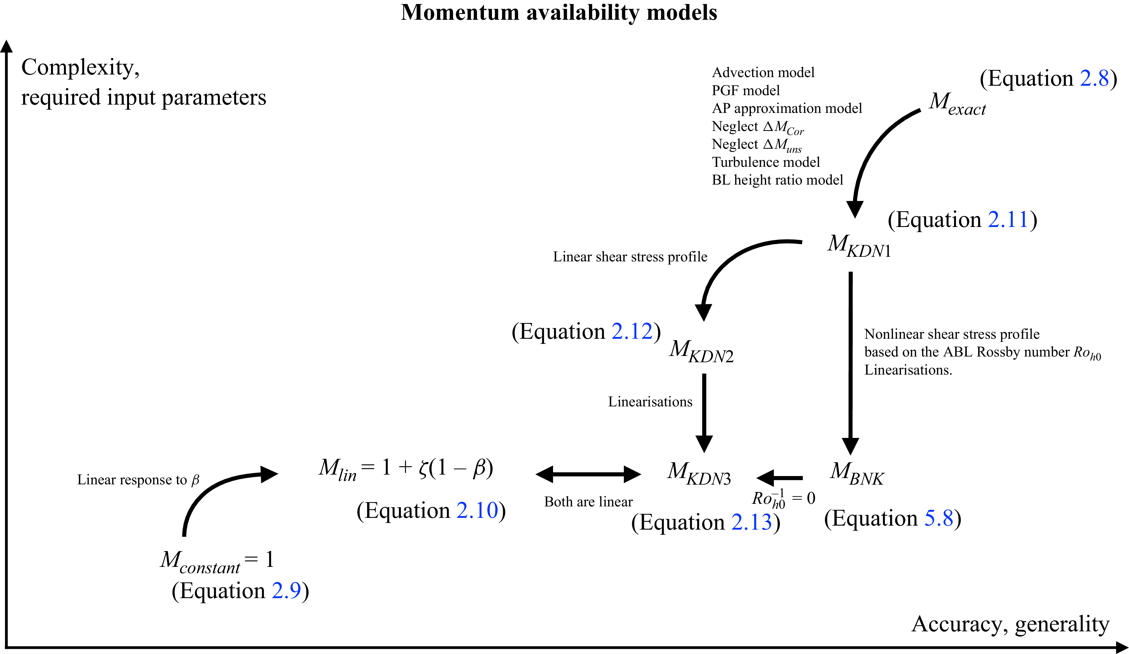
 MBNK

 Nt=160
 Nt=40
 Nt=80
 sx/D=sy/D=5
 W≡Nysy
 L≡Nxsx
 λ=NtAd/Scv=0.0314
 λ=0.00785
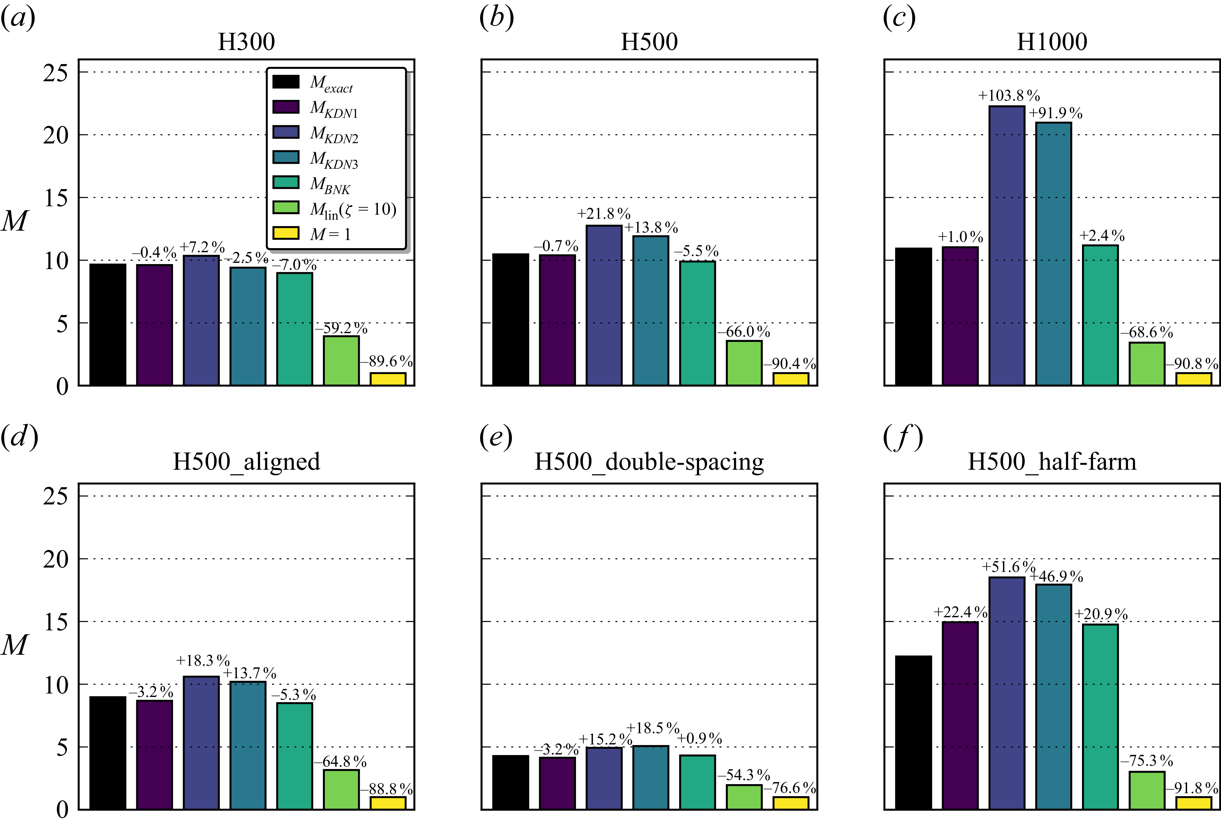
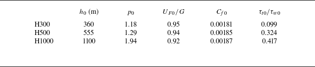
 h0
 p0
 UF0/G
 Cf0
 τt0/τw0
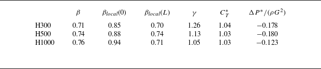
 β
 βlocal(0)
 βlocal(L)
 γ
 CT∗
 ΔP∗/(ρG2)
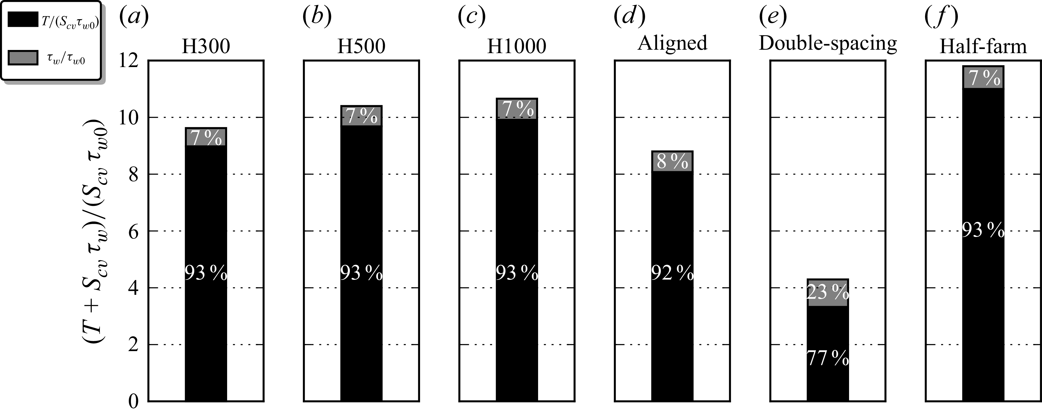

 y=[ycentre−W/2,ycentre+W/2]
 z=[0,HF]

 U1


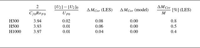
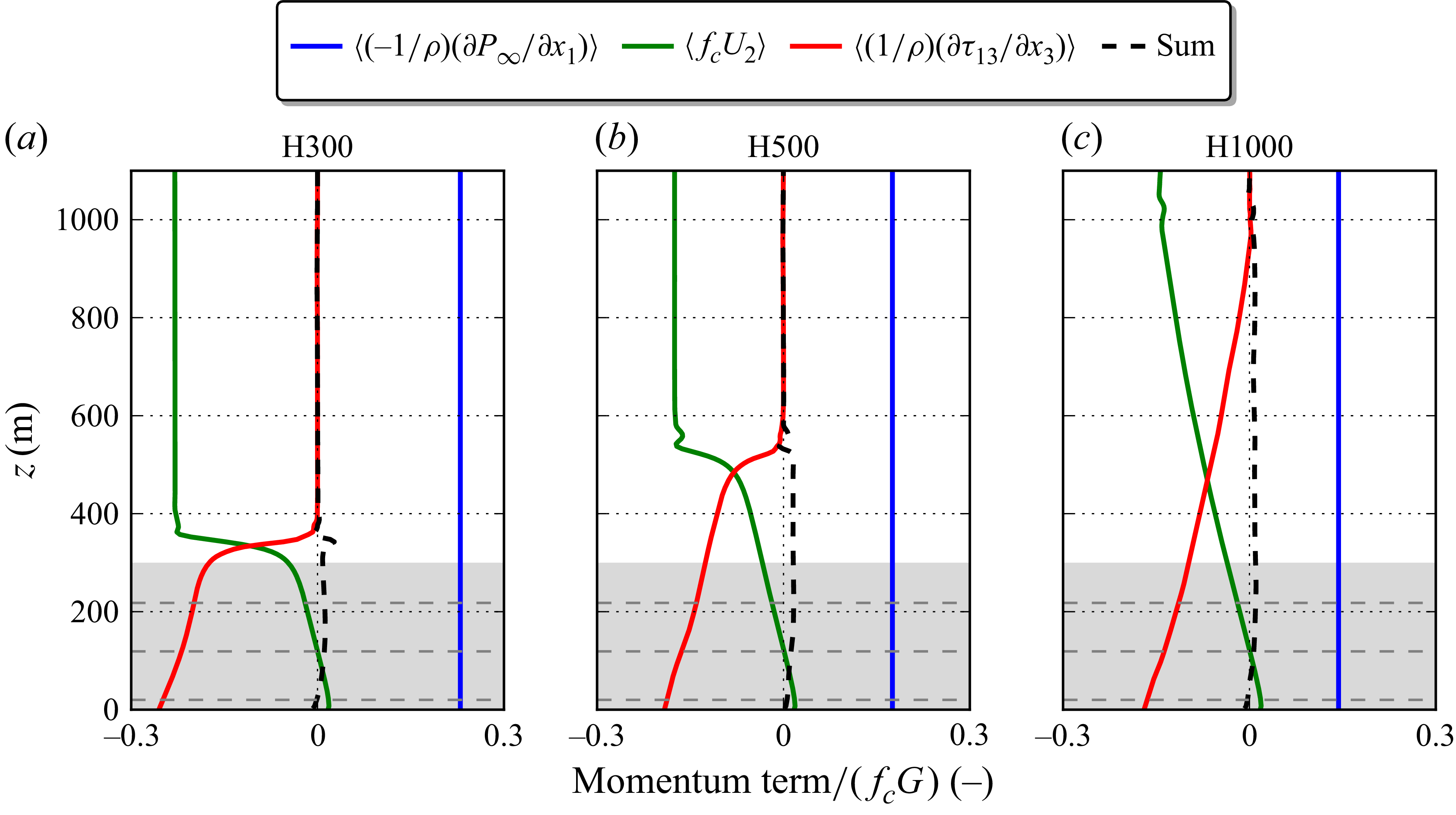


 y=[ycentre−W/2,ycentre+W/2]
 δ(x)
 (hmodel−hLES)/hLES
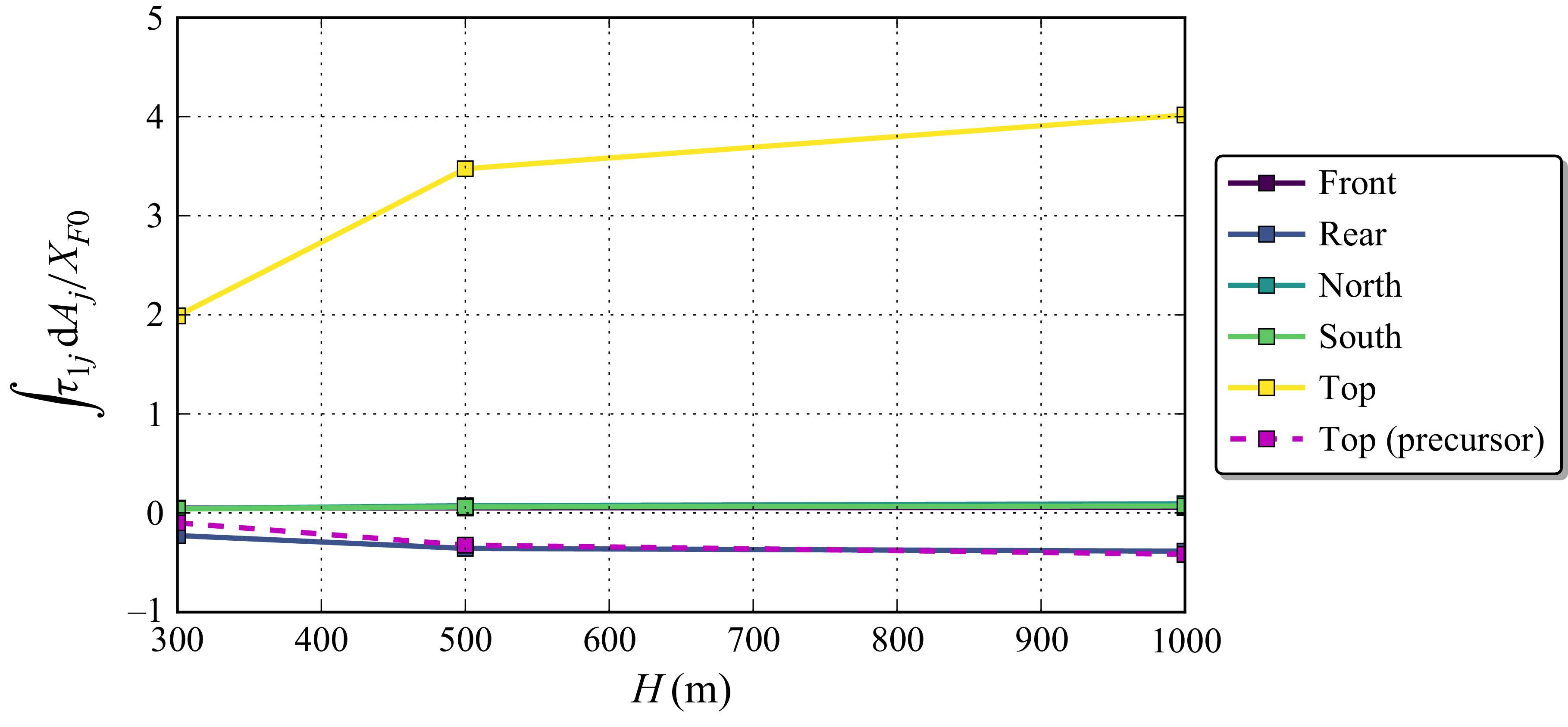
 ΔMturb

 τw1≡Mτw0
 M
 τw0
 τw0
 τw1
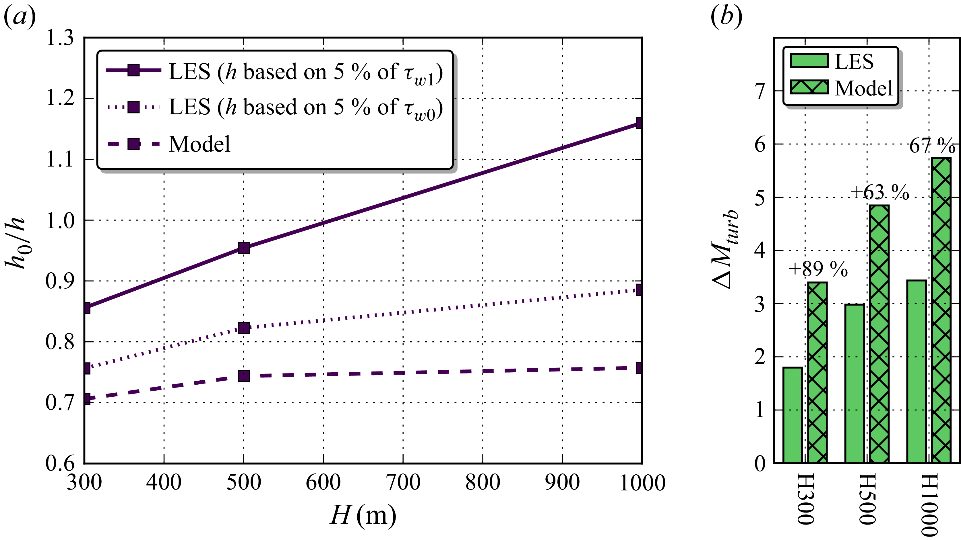
 h0/h
 h
 τw1
 h0/h=β
 h/h0
 h
 τw0
 ΔMturb

 MKDN1
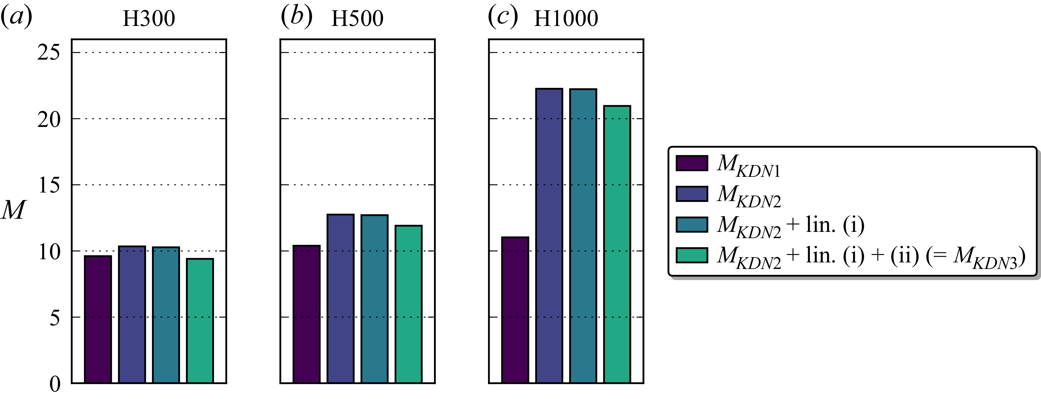
 MKDN2
 MKDN3
 MKDN1
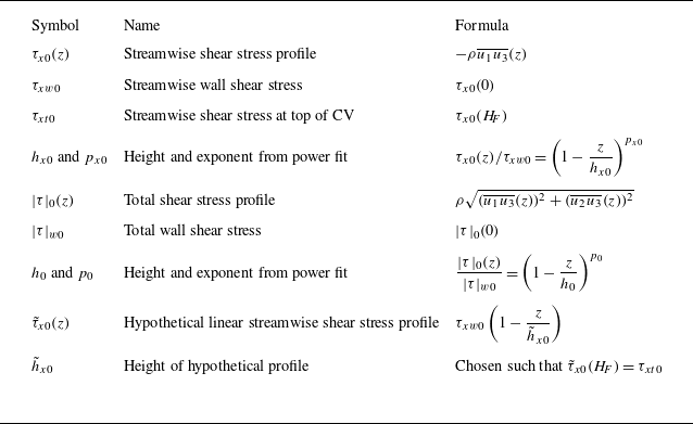
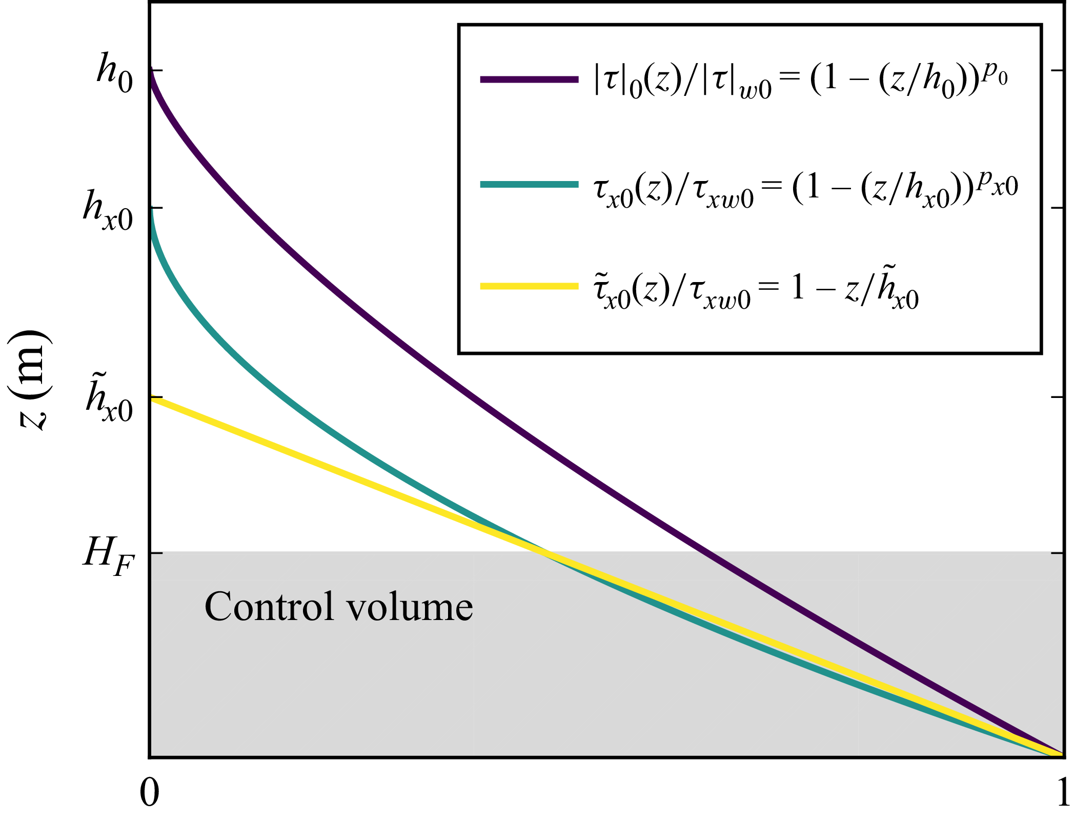
 |τ|0(z)
 τx0(z)
 τ~x0(z)
 τ~x0(HF)=τx0(HF)=τxt0

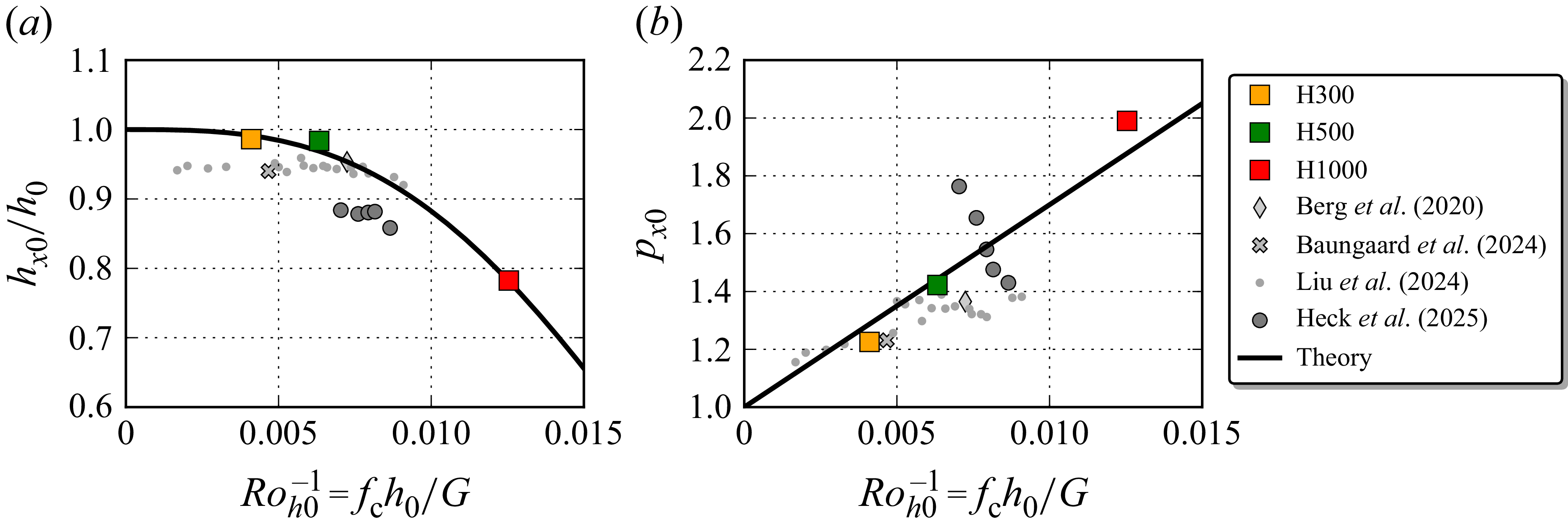
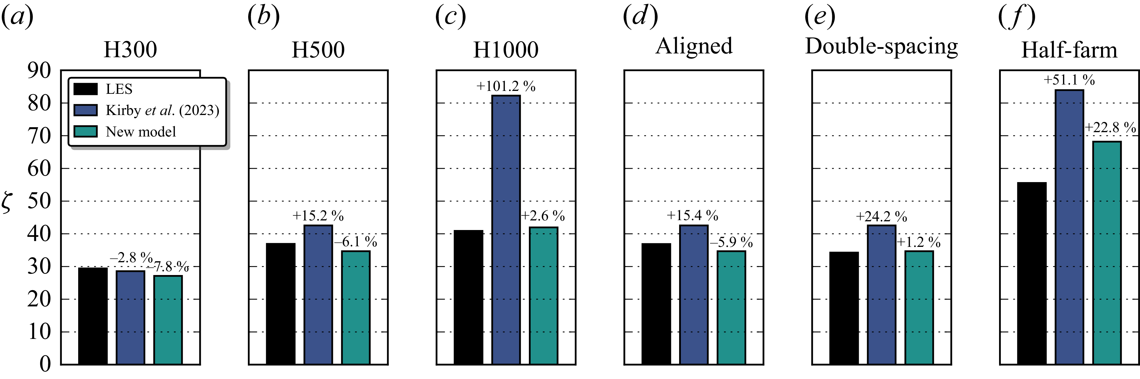
 MKDN3
 MBNK
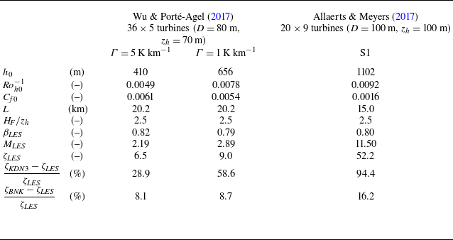
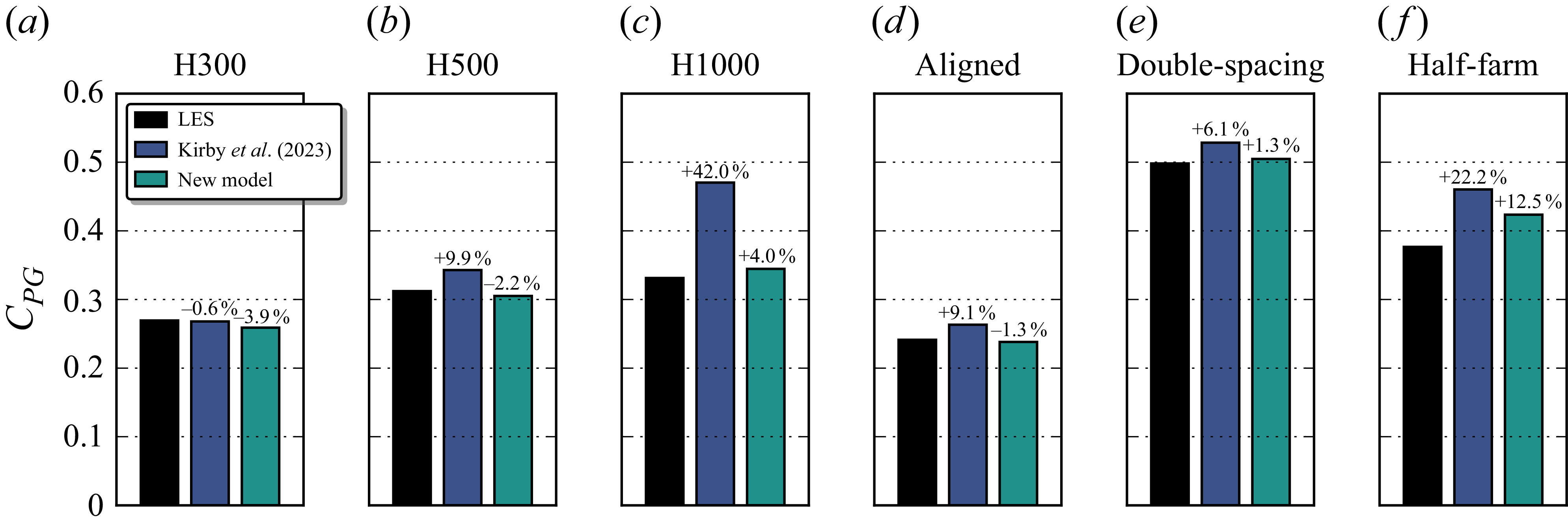
 MKDN3
 MBNK
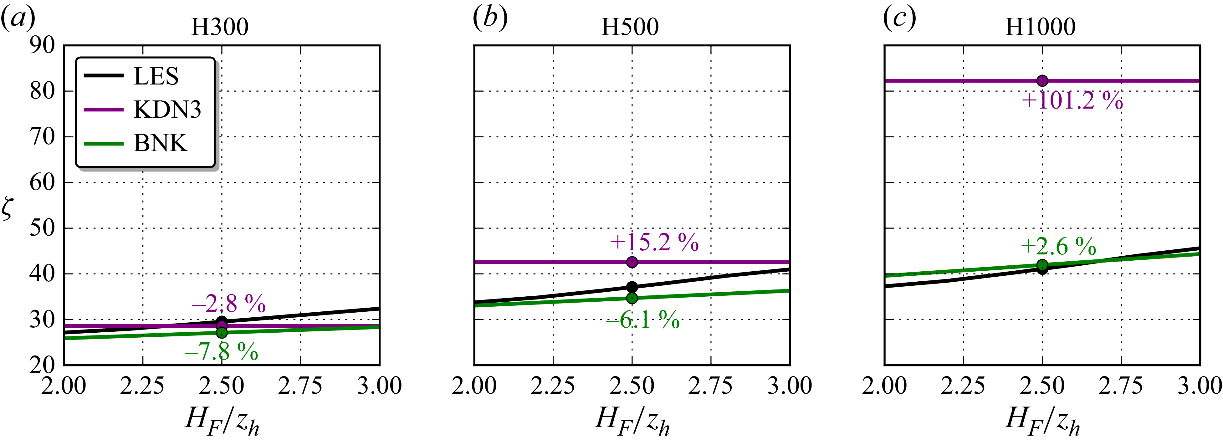
 ζLES=(MLES−1)/(1−βLES)
 ζKDN3
 ζBNK
 HF
 (∫0HFU0dz)/HF=(∫U0dA)/A
 HF/zh≈2.3
 HF/zh=2.5
 HF
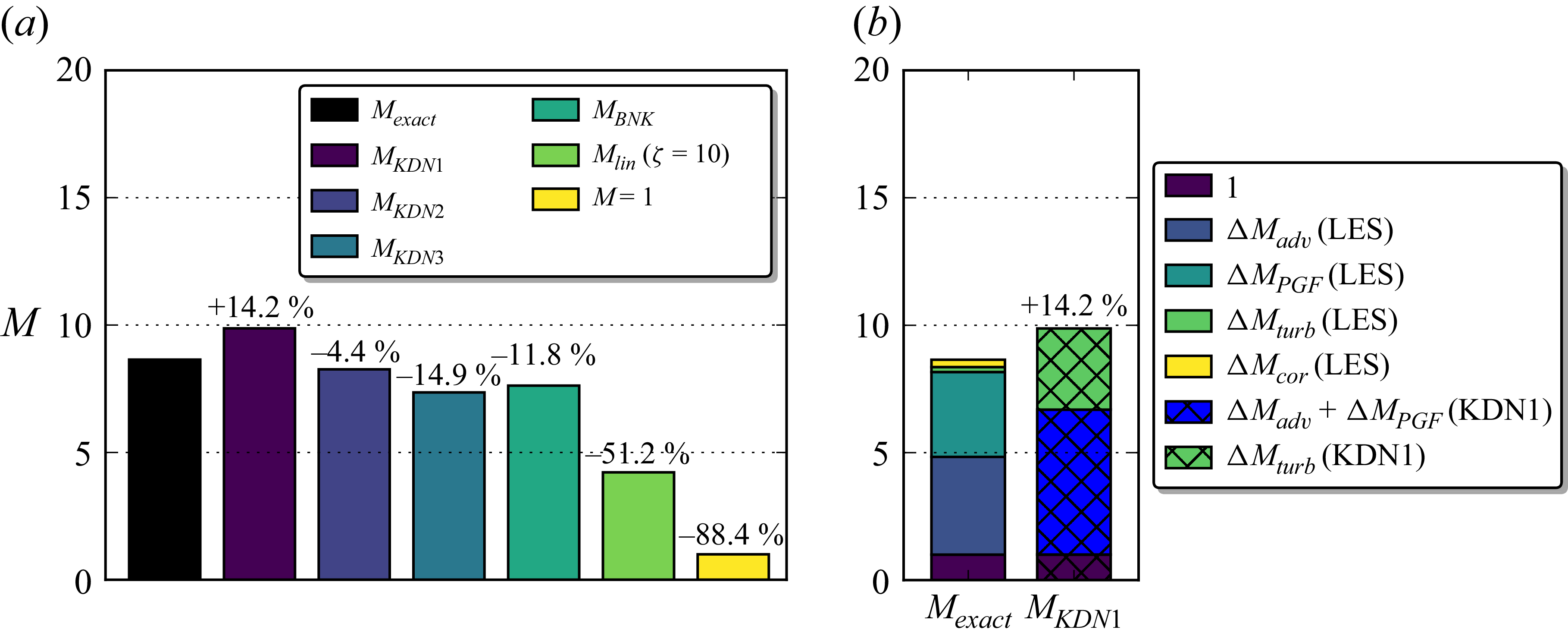

 Open access

