


1 Introduction
Recent studies report that the rate of loss of the grounded ice mass of West Antarctica has increased by
 $70\,\%$
since 2002 (Paolo, Fricker & Padman Reference Paolo, Fricker and Padman2016). A net mass loss from Antarctic ice sheets has contributed to global ocean sea level rise (Cazenave & Llovel Reference Cazenave and Llovel2010; Piecuch & Ponte Reference Piecuch and Ponte2014) and its contribution is expected to become larger in the future. Melting of glacier tongues is also contributing to a stronger fresh water layer over the Weddell Sea and this can result in reduced production of Antarctic Bottom Water, an important component in the global thermohaline circulation (Lavergne et al.
Reference Lavergne, Palter, Galbraith, Bernardello and Marinov2014). Much of the acceleration of ice loss has been attributed to increased flow or warming of circumpolar deep water entering cavities beneath floating ice shelves, where it can cause faster melting, retreat of the grounding line and a speed-up of glacier advance (Jenkins et al.
Reference Jenkins, Dutrieux, Jacobs, McPhail, Perrett, Webb and White2010; Jacobs et al.
Reference Jacobs, Jenkins, Giulivi and Dutrieux2011). The rate of melting has been studied using general circulation models (GCMs) (Beckmann & Goosse Reference Beckmann and Goosse2003; Swingedouw et al.
Reference Swingedouw, Fichefet, Huybrechts, Goosse, Driesschaert and Loutre2008; Spence et al.
Reference Spence, Griffies, England, Hogg, Saenko and Jourdain2014; Snow et al.
Reference Snow, Hogg, Sloyan and Downes2016) and the Regional Ocean Modelling System (ROMS) (Galton-Fenzi et al.
Reference Galton-Fenzi, Hunter, Coleman, Marsland and Warner2012). Modelling of the Pine Island Glacier and its grounding line, for example, has shown a tight coupling between the ice sheet interior and the surrounding ocean water properties and ablation rate (Rydt & Gudmundsson Reference Rydt and Gudmundsson2016). However, the underlying dynamics of ice melting is quite complex and poorly understood. The melting crucially involves the transport of heat and salt through a thin boundary layer at the ice face, whereas the models cited above resolve the flow field only at scales larger than
 $O(100)~\text{m}$
and rely on assumptions and parameterisations in order to invoke the roles of the convection and turbulent processes that control the melt (or ablation) rate. These parameterisations are also not coupled to the grid resolution, thereby exacerbating the uncertainty in the resulting model solutions (Morrison, Hogg & Ward Reference Morrison, Hogg and Ward2011; Gladish et al.
Reference Gladish, Holland, Holland and Price2012). In contrast turbulence-resolving simulations, such as the direct numerical simulations (DNS) recently reported by Gayen, Griffiths & Kerr (Reference Gayen, Griffiths and Kerr2016), along with theoretical modelling, serve as tools to understand the mechanisms governing the melting process. The results from theory and DNS are also likely to provide improved parameterisations for larger-scale models, thus enabling more accurate predictions of future ice-shelf melting rates.
Laboratory experiments with a small ice block, immersed in warm water with a vertical salinity gradient, showed a laminar boundary layer next to the ice face and the formation of double diffusive horizontal intrusions (Huppert & Turner Reference Huppert and Turner1978, Reference Huppert and Turner1980; Carey & Gebhart Reference Carey and Gebhart1982). Experiments on the ablation of a relatively tall (
 $O$
(1 m)) and vertical ice surface in colder and saline (35 ‰) water of uniform far-field conditions (Josberger & Martin Reference Josberger and Martin1981) achieved a turbulent boundary layer. A recent experimental study (Kerr & McConnochie Reference Kerr and Mcconnochie2015) revisited the turbulent ablation of a vertical wall with ambient water temperatures (
 $0{-}6\,^{\circ }\text{C}$
) and salinity (35 ‰) close to those of Antarctic waters, and showed that the melt rate is independent of height. The results also imply that natural convection is driven by the salinity buoyancy. Diffusion of salt to the ice interface lowers the melting temperature, allowing the ice to melt (or dissolve) even when the interface temperature is less than
 $0\,^{\circ }\text{C}$
(Woods Reference Woods1992; Kerr Reference Kerr1994; Wells & Worster Reference Wells and Worster2011; Kerr & McConnochie Reference Kerr and Mcconnochie2015).
Scaling laws for the natural convection boundary layer properties and ablation rate have been proposed for various flow scenarios. For a laminar boundary layer next to a vertical ice interface a balance between vertical advection by mean flow and lateral diffusion of solute leads to an ablation velocity that scales to the
 $-1/4$
power of the height, and the
 $1/4$
power of buoyancy anomaly, the latter predominantly provided by the salinity field (Josberger & Martin Reference Josberger and Martin1981; Carey & Gebhart Reference Carey and Gebhart1982; Nilson Reference Nilson1985; Wells & Worster Reference Wells and Worster2011). For a turbulent boundary layer, on the other hand, a turbulent parameterisation (such as the use of a constant turbulent diffusivity; Josberger & Martin Reference Josberger and Martin1981) is necessary. A recent theoretical model for dissolution (based on an established scaling for turbulent heat transfer for natural convection, Holman Reference Holman2010), predicts that the ablation velocity scales as
 $V\sim \unicode[STIX]{x0394}T_{L}^{4/3}$
, where
 $\unicode[STIX]{x0394}T_{L}=T_{w}-T_{L}$
is the difference between the ambient temperature
 $T_{w}$
and the freezing point at ambient salinity
 $T_{L}$
(Kerr & McConnochie Reference Kerr and Mcconnochie2015). The salinity dependence of
 $T_{L}$
implies that the temperature difference
 $\unicode[STIX]{x0394}T_{L}$
, and therefore the ablation rate, is determined by the transport of solute to the ice interface. The quantity
 $\unicode[STIX]{x0394}T_{L}$
is referred to as the ‘driving temperature difference’ because this temperature difference is the cause of melting and represents the source of the latent heat required for melting. However, it is not to be confused with the source of momentum, which is the solutal buoyancy. Kerr & McConnochie (Reference Kerr and Mcconnochie2015) also show that the theoretical model is consistent with earlier estimation of iceberg melt rate from ocean measurements (Morgan & Budd Reference Morgan, Budd and Husseiny1978; Budd, Jacka & Morgan Reference Budd, Jacka and Morgan1980; Shepherd, Wingham & Rignot Reference Shepherd, Wingham and Rignot2004), as well as with their own laboratory experiments.
In large-scale ice–ocean models the boundary layer turbulence is assumed to be driven by shear instability of an ambient current or buoyant plume. Where a buoyant plume is modelled it represents a contribution of natural convection at the ice–ocean interface due to either melting of the interface or a subglacial discharge of fresh water (Jenkins Reference Jenkins1991; Payne et al. Reference Payne, Holland, Shepherd, Rutt, Jenkins and Joughin2007; Jenkins Reference Jenkins2011). Plume models have used the conservation of momentum and heat (Morton, Taylor & Turner Reference Morton, Taylor and Turner1956; Ellison & Turner Reference Ellison and Turner1959) for a one-dimensional convective plume with ‘top hat’ profiles across the plume, providing a parameterisation of turbulent fluxes to the ice face. The wall plume model is further developed by incorporating the flux equation for salt transport through a solutal boundary layer under a sloping ice interface (Jenkins Reference Jenkins2011; Magorrian & Wells Reference Magorrian and Wells2016; Slater et al. Reference Slater, Goldberg, Nienow and Cowton2016). For a vertical ice face McConnochie & Kerr (Reference McConnochie and Kerr2016) have improved the model through laboratory measurements of entrainment into the turbulent plume. Like the parameterisations for the case of an ambient current, use of the plume model assumes that turbulent fluxes to the ice face are a result of instability of the mean shear in the plume.
Three-dimensional DNS of the dissolution of ice into seawater have to date focussed on natural convection alone, and a vertical planar ice face. For a range of typical Antarctic water temperatures and salinities the computed dissolution rates (Gayen et al.
Reference Gayen, Griffiths and Kerr2016) are in excellent agreement with the laboratory experiments by Josberger & Martin (Reference Josberger and Martin1981) and Kerr & McConnochie (Reference Kerr and Mcconnochie2015) and with the predicted
 $4/3$
power dependence of ablation rate on the difference between the far-field water temperature and the interface melting temperature. The DNS also showed that the ablation rate is independent of height when the boundary layer is turbulent at large values of the Grashof number, which implies that the flow is independent of further increase in the size of the computational domain. Another important result from the DNS is logarithmic profiles in velocity and density fields within the boundary layer. This is associated with production of the eddies by the mean shear at a rate comparable to that from convective instability in this vertical natural convection at the Grashof number achieved.
The focus of this paper is the effects of ice face slope on melting rates. Observations of glacier tongues on the seaward side of the grounding line indicate that the ice–water interface has a wide range of slopes (Jenkins et al. Reference Jenkins, Dutrieux, Jacobs, McPhail, Perrett, Webb and White2010). Melting near the grounding line is of particular interest, as this is where melting is most likely to influence the glacier dynamics and the overall rate of loss of grounded ice, hence sea level rise (Rignot & Jacobs Reference Rignot and Jacobs2002). Under a sloping ice face the flow and melting are expected to be complicated by a component of the buoyancy force orthogonal to the sloping face, leading to a gravitationally stable salinity stratification in the boundary layer. Attempts to describe the melting of a sloping ice boundary (Jenkins Reference Jenkins2011; Magorrian & Wells Reference Magorrian and Wells2016) have used the turbulent buoyant plume theory. However, there are no turbulence-resolving simulations to test the scaling for boundary layer properties and melting rate. The energy pathways for production of turbulence, an important consideration for the formulation of a parameterisation, are also unknown. Here we investigate the effects of slope on the ablation rate and boundary layer properties for ice in contact with uniform and quiescent surrounding seawater using scaling theory and DNS. The simulations show complex boundary layer structures and support a new scaling prediction. The energy pathways to turbulence are also examined.
2 Formulation of the problem and solution techniques
Schematic of the simulation domain. The ice face of length
 $L$
is in contact with the seawater beneath at initial temperature
 $T_{w}$
and salinity
 $S_{w}$
. At the bottom right, the domain has an open boundary condition using a sponge layer. Interface conditions at the ice (
 $T_{int}$
;
 $S_{int}$
and dissolution velocity
 $V$
) are evaluated from heat and salt flux balances at that boundary.

The flow field is solved in a rectangular domain shown in figure 1 with length
 $L$
parallel to the slope, depth
 $W$
normal to the ice face and a width
 $D$
in the spanwise direction (normal to the plane of the schematic). Ice–water interface conditions are applied at one boundary (the ice face) of the computational domain (figure 1). The domain and coordinate system are rotated relative to gravity in order to represent the ice slope. Gravity is always directed downward. The flow field is represented by
 $\tilde{\boldsymbol{u}}=[u_{\unicode[STIX]{x1D702}},v,u_{\unicode[STIX]{x1D701}}]$
, where the wall-normal (
 $\unicode[STIX]{x1D702}$
), spanwise (
 $y$
) and slope-parallel (
 $\unicode[STIX]{x1D701}$
) directions are
 $u_{\unicode[STIX]{x1D702}}$
,
 $v$
and
 $u_{\unicode[STIX]{x1D701}}$
, respectively. The coordinates and velocities are relative to a reference frame fixed at the planar ice–water interface. This is the most convenient reference frame and we make no assumption about the relative speeds of the glacier advance and ablation. We solve the incompressible continuity, Navier–Stokes, heat and salt equations:
 $$\begin{eqnarray}\displaystyle & \displaystyle \unicode[STIX]{x1D735}\boldsymbol{\cdot }\tilde{\boldsymbol{u}}=0, & \displaystyle\end{eqnarray}$$
 $$\begin{eqnarray}\displaystyle & \displaystyle \frac{\unicode[STIX]{x2202}u_{\unicode[STIX]{x1D702}}}{\unicode[STIX]{x2202}t}+(\tilde{\boldsymbol{u}}\boldsymbol{\cdot }\unicode[STIX]{x1D735})u_{\unicode[STIX]{x1D702}}=-\frac{1}{\unicode[STIX]{x1D70C}_{0}}\frac{\unicode[STIX]{x2202}p^{\ast }}{\unicode[STIX]{x2202}\unicode[STIX]{x1D702}}+\unicode[STIX]{x1D708}\unicode[STIX]{x1D6FB}^{2}u_{\unicode[STIX]{x1D702}}+\frac{\unicode[STIX]{x1D70C}^{\ast }}{\unicode[STIX]{x1D70C}_{0}}g\cos \unicode[STIX]{x1D703}, & \displaystyle\end{eqnarray}$$
 $$\begin{eqnarray}\displaystyle & \displaystyle \frac{\unicode[STIX]{x2202}u_{\unicode[STIX]{x1D701}}}{\unicode[STIX]{x2202}t}+(\tilde{\boldsymbol{u}}\boldsymbol{\cdot }\unicode[STIX]{x1D735})u_{\unicode[STIX]{x1D701}}=-\frac{1}{\unicode[STIX]{x1D70C}_{0}}\frac{\unicode[STIX]{x2202}p^{\ast }}{\unicode[STIX]{x2202}\unicode[STIX]{x1D701}}+\unicode[STIX]{x1D708}\unicode[STIX]{x1D6FB}^{2}u_{\unicode[STIX]{x1D701}}-\frac{\unicode[STIX]{x1D70C}^{\ast }}{\unicode[STIX]{x1D70C}_{0}}g\sin \unicode[STIX]{x1D703}, & \displaystyle\end{eqnarray}$$
 $$\begin{eqnarray}\displaystyle & \displaystyle \frac{\unicode[STIX]{x2202}v}{\unicode[STIX]{x2202}t}+(\tilde{\boldsymbol{u}}\boldsymbol{\cdot }\unicode[STIX]{x1D735})v=-\frac{1}{\unicode[STIX]{x1D70C}_{0}}\frac{\unicode[STIX]{x2202}p^{\ast }}{\unicode[STIX]{x2202}y}+\unicode[STIX]{x1D708}\unicode[STIX]{x1D6FB}^{2}v, & \displaystyle\end{eqnarray}$$
 $$\begin{eqnarray}\displaystyle & \displaystyle \frac{\unicode[STIX]{x2202}T^{\ast }}{\unicode[STIX]{x2202}t}+(\tilde{\boldsymbol{u}}\boldsymbol{\cdot }\unicode[STIX]{x1D735})T^{\ast }=\unicode[STIX]{x1D705}_{T}\unicode[STIX]{x1D6FB}^{2}T^{\ast }, & \displaystyle\end{eqnarray}$$
 $$\begin{eqnarray}\displaystyle & \displaystyle \frac{\unicode[STIX]{x2202}S^{\ast }}{\unicode[STIX]{x2202}t}+(\tilde{\boldsymbol{u}}\boldsymbol{\cdot }\unicode[STIX]{x1D735})S^{\ast }=\unicode[STIX]{x1D705}_{S}\unicode[STIX]{x1D6FB}^{2}S^{\ast }. & \displaystyle\end{eqnarray}$$
Here
 $\unicode[STIX]{x1D70C}_{0}$
is the reference density for pure water at
 $0\,^{\circ }$
C and
 $p^{\ast },T^{\ast },S^{\ast }$
and
 $\unicode[STIX]{x1D70C}^{\ast }$
denote the deviation from the ambient hydrostatic pressure
 $(p_{w})$
, temperature
 $(T_{w})$
, salinity
 $(S_{w})$
and density
 $(\unicode[STIX]{x1D70C}_{w})$
. The saline water has kinematic viscosity
 $\unicode[STIX]{x1D708}$
, thermal diffusivity
 $\unicode[STIX]{x1D705}_{T}$
and salinity diffusivity
 $\unicode[STIX]{x1D705}_{S}$
. As the flow involves only a small range of temperatures, the equation of state is closely approximated as linear without significant effects on the solution:
 $$\begin{eqnarray}\displaystyle \unicode[STIX]{x1D70C}^{\ast }=\unicode[STIX]{x1D70C}_{0}(\unicode[STIX]{x1D6FD}S^{\ast }-\unicode[STIX]{x1D6FC}T^{\ast }), & & \displaystyle\end{eqnarray}$$
with coefficient of thermal expansion
 $\unicode[STIX]{x1D6FC}$
and coefficient of haline contraction
 $\unicode[STIX]{x1D6FD}$
. Computational domains of a given length but different slopes have different vertical heights. Thus we compare the flow and melt rate for different slopes at two given values of the global Grashof number (
 $Gr$
, which is the relative strength of buoyancy to viscous force) and one value of the Stefan number (
 $St$
),
 $$\begin{eqnarray}\displaystyle Gr\equiv \frac{g\unicode[STIX]{x1D6FD}\unicode[STIX]{x0394}SL^{3}}{\unicode[STIX]{x1D708}^{2}},\quad St\equiv \frac{\unicode[STIX]{x1D70C}_{s}L_{f}}{\unicode[STIX]{x1D70C}_{w}c_{w}(T_{w}-T_{int})}, & & \displaystyle\end{eqnarray}$$
where, [
 $S_{int},T_{int}$
] are the interface and [
 $S_{w},T_{w}$
] are the far-field salinity and temperature,
 $\unicode[STIX]{x0394}S=(S_{w}-S_{int})$
is the salinity anomaly,
 $c_{w}$
is the specific heat,
 $L_{f}$
is the latent heat of fusion for ice and
 $\unicode[STIX]{x1D70C}_{s}$
is the density of the ice. The values of
 $Gr$
and
 $St$
are independent of slope because the simulations in § 4 show that the interface temperature and salinity are independent of slope. The Prandtl number (
 $Pr=\unicode[STIX]{x1D708}/\unicode[STIX]{x1D705}_{T}$
) and Schmidt number (
 $Sc=\unicode[STIX]{x1D708}/\unicode[STIX]{x1D705}_{S}$
) are fixed.
Three relations are applied at the ice–water interface. The freezing point of saline water is closely approximated by a linear function of salinity and pressure:
 $$\begin{eqnarray}\displaystyle T_{int}=a_{s}S_{int}+bP_{int}\simeq a_{s}S_{int}. & & \displaystyle\end{eqnarray}$$
For the present study the effect on the freezing point of hydrostatic pressure difference within the limited domain size is negligible and the interface temperature is assumed to be solely dependent on interface salinity. The slope of the liquidus line is fixed at a s = -6 × 10⁻² °C ‰-1 (Holland & Jenkins Reference Holland and Jenkins1999).
The second interface relation expresses the balance between latent heat flux
 $Q_{m}^{H}$
of melting and the divergence of conductive heat fluxes at the interface,
 $$\begin{eqnarray}\displaystyle Q_{ice}^{H}-Q_{w}^{H}=Q_{m}^{H}, & & \displaystyle\end{eqnarray}$$
where
 $Q_{ice}^{H}$
and
 $Q_{w}^{H}$
are the heat fluxes to the interface in the ice and water, respectively. The conductive transfer of heat into the ice is very small compared to the total heat being used to melt the ice shelf under typical Antarctic conditions (Holland & Jenkins Reference Holland and Jenkins1999; Kerr & McConnochie Reference Kerr and Mcconnochie2015). We therefore neglect the diffusive heat flux into the ice (setting
 $Q_{ice}^{H}\sim 0$
). It is also assumed that the diffusion of heat in water at the interface is much faster than the advection of heat by the ablation velocity (i.e.
 $\unicode[STIX]{x1D705}_{T}\unicode[STIX]{x2202}^{2}T/\unicode[STIX]{x2202}\unicode[STIX]{x1D702}^{2}\gg V\unicode[STIX]{x2202}T/\unicode[STIX]{x2202}\unicode[STIX]{x1D702}|_{\unicode[STIX]{x1D702}=0}$
, as
 $V\ll \unicode[STIX]{x1D705}_{T}/\unicode[STIX]{x1D6FF}_{T}$
, where
 $\unicode[STIX]{x1D6FF}_{T}$
is the diffusive thermal boundary layer thickness), so that (2.10) becomes
 $$\begin{eqnarray}\displaystyle \left.\unicode[STIX]{x1D70C}_{w}c_{w}\unicode[STIX]{x1D705}_{T}\frac{\unicode[STIX]{x2202}T}{\unicode[STIX]{x2202}\unicode[STIX]{x1D702}}\right|_{\unicode[STIX]{x1D702}=0}=\unicode[STIX]{x1D70C}_{s}VL_{f}, & & \displaystyle\end{eqnarray}$$
where
 $V$
is the ablation velocity. We adopt the convention that positive ablation velocity indicates melting and retreat of the interface in the negative
 $\unicode[STIX]{x1D702}$
-direction (at speed
 $V$
) relative to the ice mass, or equivalently, translation of the ice mass in the positive
 $\unicode[STIX]{x1D702}$
-direction relative to the interface reference frame used here.
An analogous equation is used to describe the salt flux balance at the interface due to fresh water release and salt flux divergence:
 $$\begin{eqnarray}\displaystyle Q_{ice}^{S}-Q_{w}^{S}=Q_{m}^{S}. & & \displaystyle\end{eqnarray}$$
Here
 $Q_{ice}^{S}$
and
 $Q_{w}^{S}$
are the diffusive salt fluxes at the interface on the ice and water sides, respectively, and
 $Q_{m}^{S}$
is the advective fresh water flux associated with melting. The latter can be expressed as
 $Q_{m}^{S}=\unicode[STIX]{x1D70C}_{s}V(S_{ice}-S_{int})$
. The diffusive salt flux in the ice is neglected and (2.12) becomes
 $$\begin{eqnarray}\displaystyle \left.\unicode[STIX]{x1D70C}_{w}\unicode[STIX]{x1D705}_{S}\frac{\unicode[STIX]{x2202}S}{\unicode[STIX]{x2202}\unicode[STIX]{x1D702}}\right|_{\unicode[STIX]{x1D702}=0}=\unicode[STIX]{x1D70C}_{s}V(S_{int}-S_{ice}). & & \displaystyle\end{eqnarray}$$
Thus there is a balance between the diffusive flux of salt toward the ice and the advective flux of salt away from the ice face (due to the fresh water release by melting). This is in contrast to the neglect of the heat advection as discussed above. For the solutions found here we will assume that the ice is free of salt (
 $S_{ice}=0$
).
In the DNS we impose wall-normal velocity
 $u_{\unicode[STIX]{x1D702}}=\unicode[STIX]{x1D70C}_{S}V/\unicode[STIX]{x1D70C}_{w}$
(Wells & Worster Reference Wells and Worster2011) at the ice face. Effects of any mean gradient
 $\text{d}u_{\unicode[STIX]{x1D702}}/\text{d}\unicode[STIX]{x1D701}|_{\unicode[STIX]{x1D702}=0}$
(which occurs in the laminar boundary layer cases, where
 $V$
is dependent on
 $\unicode[STIX]{x1D701}$
) are neglected as justified by Carey & Gebhart (Reference Carey and Gebhart1982). Also neglected are the effects of spatial (in
 $\unicode[STIX]{x1D701}$
and
 $y$
) and temporal variations of
 $u_{\unicode[STIX]{x1D701}}|_{\unicode[STIX]{x1D702}=0}$
associated with the flow fluctuations. It was verified that the DNS solutions are unchanged even when
 $u_{\unicode[STIX]{x1D702}}|_{\unicode[STIX]{x1D702}=0}$
is everywhere set to zero.
The ‘open ocean’ side of the computational domain is maintained as an open boundary by relaxing temperature and salinity back to its background temperature
 $T_{w}$
and salinity
 $S_{w}$
, respectively, through a ‘sponge’ region (Gayen & Sarkar Reference Gayen and Sarkar2011) at
 $0.5W\leqslant \unicode[STIX]{x1D702}\leqslant W$
. The along-slope, spanwise velocities and scalar fields are relaxed towards the background state in the sponge region by adding damping functions
 $-\unicode[STIX]{x1D70E}(\unicode[STIX]{x1D702})u_{i}(\unicode[STIX]{x1D702},y,\unicode[STIX]{x1D701},t)$
(
 $i=2,3$
),
 $-\unicode[STIX]{x1D70E}(\unicode[STIX]{x1D702})T^{\ast }(\unicode[STIX]{x1D702},y,\unicode[STIX]{x1D701},t)$
and
 $-\unicode[STIX]{x1D70E}(\unicode[STIX]{x1D702})S^{\ast }(\unicode[STIX]{x1D702},y,\unicode[STIX]{x1D701},t)$
to the right-hand side of the momentum and scalar equations, respectively, where
 $\unicode[STIX]{x1D70E}(\unicode[STIX]{x1D702})$
is based on the time step
 $\unicode[STIX]{x0394}t$
and changes from 0 at
 $\unicode[STIX]{x1D702}=0.5W$
to
 $1/\unicode[STIX]{x0394}t$
 $\text{s}^{-1}$
at
 $\unicode[STIX]{x1D702}=W$
. At the down-slope and up-slope boundaries of the domain, no-slip conditions are imposed for velocities and no-flux conditions are maintained for the temperature and salinity. Both
 $T_{int}$
and
 $S_{int}$
vary with location and time on the ice interface due to turbulent variations in the local heat and solute transport to the interface.
The solution is obtained using a mixed spectral/finite difference algorithm (Gayen et al.
Reference Gayen, Griffiths and Kerr2016). The wall-normal and slope-parallel spatial derivatives (
 $\unicode[STIX]{x1D702}$
and
 $\unicode[STIX]{x1D701}$
) are computed with second-order finite difference. The spanwise (
 $y$
) direction is considered periodic and derivatives in this direction are treated with a pseudo-spectral method. Time stepping is accomplished with a mixed implicit/explicit strategy with all terms involving viscous contribution being stepped with the alternating direction implicit (ADI) method. All the other terms are treated with a low storage third-order Runge–Kutta method (Gayen Reference Gayen2012).
The physical dimension of the rectangular domain for one set of simulations is
 $W=0.4~\text{m}$
,
 $D=0.05~\text{m}$
and
 $L=1.8~\text{m}$
. Additional simulations with the across-slope width doubled to
 $D=0.1~\text{m}$
, and the same
 $W$
and
 $L$
, show similar boundary layer properties and melt rates. Thus a width of
 $D=0.05~\text{m}$
is used for the remainder of the simulations for the sake of computational efficiency. A second set of solutions in a larger domain used
 $W=4~\text{m}$
,
 $D=0.05~\text{m}$
and
 $L=20~\text{m}$
. In the two domain lengths the grids have
 $256\times 64\times 1150$
and
 $256\times 64\times 1920$
points in the
 $\unicode[STIX]{x1D702}$
,
 $y$
and
 $\unicode[STIX]{x1D701}$
directions, respectively. In order to resolve the salinity boundary layer and turbulent microscales for salinity, grid stretching is used in the
 $\unicode[STIX]{x1D702}$
direction. All solutions satisfy rigorous grid resolution and grid convergence criteria that are reported in detail in Gayen, Griffiths & Hughes (Reference Gayen, Griffiths and Hughes2014), Gayen et al. (Reference Gayen, Griffiths and Kerr2016). Variable time stepping with a fixed Courant–Friedrichs–Lewy (CFL) number of
 $N_{CFL}=0.5$
is used. The time step is calculated to be
 $\unicode[STIX]{x0394}t=(1/N_{CFL})[\unicode[STIX]{x0394}\unicode[STIX]{x1D702}/u_{\unicode[STIX]{x1D702}},\unicode[STIX]{x0394}y/v,\unicode[STIX]{x0394}\unicode[STIX]{x1D701}/u_{\unicode[STIX]{x1D701}}]_{min}$
and varies significantly, from
 $O(10^{-3})~\text{s}$
in the turbulent regime to
 $O(10^{-2})~\text{s}$
in the laminar regime. The fractional step method is used to evaluate dynamic pressure at each time step (Gayen & Sarkar Reference Gayen and Sarkar2011).
The slope angle
 $\unicode[STIX]{x1D703}$
is varied from
 $2^{\circ }$
to
 $90^{\circ }$
. In order to focus on the effect of slope on the melting process, the far-field temperature
 $T_{w}=2.3^{\circ }\text{C}$
and salinity S
w
= 35 ‰ are fixed for all cases. All temperatures are measured with respect to the freezing point of pure water and therefore are quoted in Celsius. We fix
 $g=10~\text{m}~\text{s}^{-2}$
,
 $\unicode[STIX]{x1D705}_{T}=1.285\times 10^{-7}~\text{m}^{2}~\text{s}^{-1}$
,
 $c_{w}=3985~\text{J}~\text{kg}^{-1}~\text{K}^{-1}$
,
 $\unicode[STIX]{x1D708}=1.8\times 10^{-6}~\text{m}^{2}~\text{s}^{-1}$
,
 $\unicode[STIX]{x1D6FC}=6\times 10^{-5}~\text{K}^{-1}$
and 𝛽 = 8 × 10⁻⁴ ‰-1, taken from the physical properties of aqueous NaCl solutions at the far-field temperature and salinity (Washburn Reference Washburn1926; Weast, Astle & Beyer Reference Weast, Astle and Beyer1989). We use
 $\unicode[STIX]{x1D705}_{S}=7.2\times 10^{-10}~\text{m}^{2}~\text{ s}^{-1}$
at
 $0^{\circ }\text{C}$
(Josberger & Martin Reference Josberger and Martin1981) with a resultant
 $Sc=2500$
at grid points adjacent to the interface. In the interior we use
 $\unicode[STIX]{x1D705}_{S}=3.6\times 10^{-9}~\text{m}^{2}~\text{s}^{-1}$
(
 $Sc=500$
, Gayen et al.
Reference Gayen, Griffiths and Kerr2016) in order to make the turbulence simulations feasible. The Prandtl number is fixed at
 $Pr=15$
throughout the domain. The primary solution sets are designed to cover the range of slope angles for both
 $Gr=7.5\times 10^{11}$
(for a domain length of 1.8 m) and
 $Gr=10.28\times 10^{14}$
(domain length of 20 m).
The critical Grashof number for transitions from laminar to turbulent flow on a vertical wall varies from
 $Gr_{c}^{\bot }\sim 10^{9}{-}10^{10}$
(Turner Reference Turner1979; Josberger & Martin Reference Josberger and Martin1981; Holman Reference Holman2010). A first approximation for the critical along-slope distance
 $L_{c}$
beyond which the boundary layer becomes turbulent, based on the critical vertical height
 $L_{c}^{\bot }$
, is
 $$\begin{eqnarray}\displaystyle L_{c}\approx \frac{L_{c}^{\bot }}{\sin \unicode[STIX]{x1D703}}=\frac{1}{\sin \unicode[STIX]{x1D703}}\left(\frac{\unicode[STIX]{x1D708}^{2}Gr_{c}^{\bot }}{g\unicode[STIX]{x1D6FD}\unicode[STIX]{x0394}S}\right)^{1/3}, & & \displaystyle\end{eqnarray}$$
giving a critical Grashof number for the sloping interface as
 $$\begin{eqnarray}\displaystyle Gr_{c}\approx \frac{Gr_{c}^{\bot }}{(\sin \unicode[STIX]{x1D703})^{3}}. & & \displaystyle\end{eqnarray}$$
Based on this assumption we calculated the transition length for various slope angles bounding the previously established critical
 $Gr_{c}^{\bot }$
(figure 2) and plotted the laminar to turbulent transition length (
 $L_{c}$
) given by the DNS, where
 $L_{c}$
is defined as the height where spanwise fluctuations (
 $v_{rms}$
,
 $rms$
 $=$
root mean square) reach 10 % or more of the average up-slope flow. The results show that the along-slope length required to achieve turbulence increases rapidly with decreasing slope angles. Hence we require the longer domain of
 $20$
m in order to simulate turbulent conditions under sloping ice at
 $\unicode[STIX]{x1D703}\leqslant 20^{\circ }$
.
3 Scaling analysis
Ablation of the ice face takes place when it is in contact with saline water with a temperature greater than the melting temperature. The addition of melt water to the saline water results in freshening of a layer adjacent to the ice and gives rise to a buoyant boundary layer plume. Working from the momentum and solute transport equations the plume can be divided into multiple layers (figure 3) based on the dominant balances discussed below. The buoyancy force is important only within a solutal boundary layer at the ice face, of thickness
 $\unicode[STIX]{x1D6FF}_{S}$
, and we refer to this as the ‘inner layer’. Diffusion or turbulent advection of heat in the wall-normal direction is important within a thermal boundary layer of thickness
 $\unicode[STIX]{x1D6FF}_{T}$
. However, the thermal buoyancy is relatively small and does not enter the momentum balance at leading order. In the inner layer, solutal buoyancy and stress are the dominant terms in the momentum equation. Outside the inner boundary layer there is an outer layer, of thickness
 $\unicode[STIX]{x1D6FF}_{0}$
, in which buoyancy forces make a negligible contribution.
When the flow is laminar the whole of the inner layer will be dominated by the balance of buoyancy with molecular viscous stress, and by molecular diffusion of heat and solute toward the ice, as previously described in the context of a vertical ice face (Wells & Worster Reference Wells and Worster2011). The laminar outer layer is governed by an inertia–viscous balance. That analysis is adapted here (§ 3.1) to a sloping ice face. We find that this laminar solution may have geophysical relevance for very small ice slopes, as a consequence of a stabilising density stratification produced by the melting.
Simulated and theoretically predicted (2.14) laminar to turbulent transition length, where the predictions (curves) are based on the critical Grashof number for a vertical wall (
 $Gr_{c}^{\bot }=10^{9}{-}10^{10}$
). The simulated transition length
 $L_{t}$
is calculated based on turbulent statistics from the simulations for
 $L=1.8~\text{m}$
and 20 m, respectively.

Schematic of the theoretical model boundary layer structure, with up-slope velocity and solute concentration profiles in the wall-normal direction, for the case of a turbulent plume (thicknesses not to scale).

When the plume is turbulent, small-scale eddies add significantly to momentum transport in the wall-normal direction within the buoyant inner layer, leaving a much thinner laminar and diffusive sublayer (of thickness
 $\unicode[STIX]{x1D6FF}_{sub}$
) on the ice face. Within the sub-layer eddy transport and turbulent kinetic energy production are negligible. The smallness of the sub-layer thickness is confirmed by the DNS solutions reported here, which show it to be
 $O(10)$
times smaller than the inner layer thickness
 $\unicode[STIX]{x1D6FF}_{S}$
. In the inner layer the dominant momentum balance is between the solutal buoyancy and Reynolds stress. However, scaling indicates that the molecular diffusion of solute toward the ice remains a dominant term in the salt budget. In the outer layer the turbulent plume is dominated by Reynolds stress and turbulent transport of solute, leaving the solute relatively well mixed, which in turn implies a negligible molecular transport of solute. Molecular diffusion of heat can remain important throughout a region of thickness
 $\unicode[STIX]{x1D6FF}_{T}$
, which may overlap the outer inertial layer. Ambient fluid is entrained into the turbulent plume from the edge of the outer layer. The layers defined here are consistent with a model previously proposed for thermal convection at a heated vertical boundary (Wells & Worster Reference Wells and Worster2008). In the following sub-sections the thicknesses of the sloping inner solutal layer and thermal boundary layer, and the ablation rate, are analysed for laminar and turbulent cases.
3.1 Laminar boundary layer flows: viscous–buoyancy balance
Wells & Worster (Reference Wells and Worster2011) derived similarity solutions for melting and dissolving with a laminar boundary layer for a vertical ice face and quiescent far field. (The final form of the similarity solution for the case of dissolution of a solute at a vertical wall was also quoted by Husband & Ozsahin (Reference Husband and Ozsahin1967). Here we summarise their solution for the case of dissolving and extend it to sloping ice faces. However, for brevity we use simple scaling arguments, which also assist in contrasting the dynamics of laminar and turbulent cases.) In the inner layer
 $\unicode[STIX]{x1D6FF}_{S}$
and
 ${\mathcal{L}}$
are the characteristic length scales for the wall-normal and the along-slope directions, respectively, whereas
 $\unicode[STIX]{x1D6FF}_{0}$
and
 ${\mathcal{L}}$
are the characteristic length scales associated with the outer layer. At small Grashof numbers (
 $Gr<Gr_{c}$
) or shallow slopes, the inertia terms inside the diffusive boundary layer are negligible, leaving a balance between viscous drag and buoyancy in the up-slope flow in the momentum equations (2.2)–(2.4). The buoyancy is predominantly supplied by the salinity anomaly (
 $\unicode[STIX]{x0394}S$
) across the diffusive boundary layer:
 $$\begin{eqnarray}\displaystyle \unicode[STIX]{x1D708}\frac{\unicode[STIX]{x2202}^{2}U_{\unicode[STIX]{x1D701}}}{\unicode[STIX]{x2202}\unicode[STIX]{x1D702}^{2}}\sim \unicode[STIX]{x1D708}\frac{U_{\unicode[STIX]{x1D701}}}{\unicode[STIX]{x1D6FF}_{S}^{2}}\sim g\sin \unicode[STIX]{x1D703}\unicode[STIX]{x1D6FD}\unicode[STIX]{x0394}S. & & \displaystyle\end{eqnarray}$$
The scaling of the viscous terms in (3.1) holds for large
 $Sc$
, as the inflection in the up-slope velocity profile must lie outside the buoyancy-driven inner layer. The wall-normal derivatives in the boundary layer are the dominant contributions (i.e.
 $\unicode[STIX]{x2202}/\unicode[STIX]{x2202}\unicode[STIX]{x1D702}\gg \unicode[STIX]{x2202}/\unicode[STIX]{x2202}\unicode[STIX]{x1D701}$
as
 $\unicode[STIX]{x1D6FF}_{S}\ll {\mathcal{L}}$
) to both the viscous drag and the diffusion of solute. Outside the solutal diffusive boundary layer the buoyancy force is neglected and hence the inertia in the outer layer balances the residual viscous drag force generated by the up-slope flow (Nilson Reference Nilson1985). This leads to
 $$\begin{eqnarray}\displaystyle \frac{U_{\unicode[STIX]{x1D701}}^{2}}{{\mathcal{L}}}\sim \unicode[STIX]{x1D708}\frac{U_{\unicode[STIX]{x1D701}}}{\unicode[STIX]{x1D6FF}_{0}^{2}}. & & \displaystyle\end{eqnarray}$$
The convective salt transport by mean flow in (2.6) balances solute diffusion through the inner boundary layer:
 $$\begin{eqnarray}\displaystyle U_{\unicode[STIX]{x1D701}}\frac{\unicode[STIX]{x0394}S}{{\mathcal{L}}}\sim U_{\unicode[STIX]{x1D702}}\frac{\unicode[STIX]{x0394}S}{\unicode[STIX]{x1D6FF}_{S}}\sim \unicode[STIX]{x1D705}_{S}\frac{\unicode[STIX]{x0394}S}{\unicode[STIX]{x1D6FF}_{S}^{2}}. & & \displaystyle\end{eqnarray}$$
Here total velocity
 $u_{i}=U_{i}+u_{i}^{\prime }$
is decomposed into the mean boundary layer flow
 $U_{i}$
and fluctuating velocity component
 $u_{i}^{\prime }$
with the latter assumed to play a negligible role for laminar flow. We also assume that the salinity anomaly in the along-slope direction is equivalent to the salinity difference across the boundary layer. Combining (3.1) and (3.3) leads to the scaling of the thickness of the solutal boundary layer as
 $$\begin{eqnarray}\displaystyle \unicode[STIX]{x1D6FF}_{S}\sim \unicode[STIX]{x1D6FF}_{S0}(\sin \unicode[STIX]{x1D703})^{-(1/4)}, & & \displaystyle\end{eqnarray}$$
where
 $\unicode[STIX]{x1D6FF}_{S0}$
is the salinity boundary layer thickness for the case of a vertical ice face
 $$\begin{eqnarray}\displaystyle \unicode[STIX]{x1D6FF}_{S0}\sim \left(\frac{\unicode[STIX]{x1D708}\unicode[STIX]{x1D705}_{S}{\mathcal{L}}}{g\unicode[STIX]{x1D6FD}\unicode[STIX]{x0394}S}\right)^{1/4}, & & \displaystyle\end{eqnarray}$$
or equivalently,
 $$\begin{eqnarray}\displaystyle \frac{\unicode[STIX]{x1D6FF}_{S0}}{{\mathcal{L}}}\sim Gr_{{\mathcal{L}}}^{-1/4}Sc^{-1/4}, & & \displaystyle\end{eqnarray}$$
with the local Grashof number
 $Gr_{{\mathcal{L}}}=g\unicode[STIX]{x1D6FD}\unicode[STIX]{x0394}S{\mathcal{L}}^{3}/\unicode[STIX]{x1D708}^{2}$
(which is based on the up-slope distance
 ${\mathcal{L}}$
). From (2.13) the ablation rate can be estimated as
 $V\sim (\unicode[STIX]{x1D70C}_{w}\unicode[STIX]{x1D705}_{S}\unicode[STIX]{x0394}S)/(\unicode[STIX]{x1D70C}_{S}S_{int}\unicode[STIX]{x1D6FF}_{S})$
, which gives
 $$\begin{eqnarray}\displaystyle V\sim V_{0}(\sin \unicode[STIX]{x1D703})^{1/4}, & & \displaystyle\end{eqnarray}$$
where
 $V_{0}$
is the ablation rate for a vertical ice face given by
 $$\begin{eqnarray}\displaystyle V_{0}\sim \frac{\unicode[STIX]{x1D70C}_{w}\unicode[STIX]{x0394}S}{\unicode[STIX]{x1D70C}_{S}S_{int}}\left(\frac{g\unicode[STIX]{x1D6FD}\unicode[STIX]{x0394}S\unicode[STIX]{x1D705}_{S}^{3}}{\unicode[STIX]{x1D708}}\right)^{1/4}{\mathcal{L}}^{-1/4}, & & \displaystyle\end{eqnarray}$$
or
 $$\begin{eqnarray}\displaystyle \frac{V_{0}{\mathcal{L}}}{\unicode[STIX]{x1D705}_{S}}\sim \left(\frac{\unicode[STIX]{x1D70C}_{w}\unicode[STIX]{x0394}S}{\unicode[STIX]{x1D70C}_{S}S_{int}}\right)Gr_{{\mathcal{L}}}^{1/4}. & & \displaystyle\end{eqnarray}$$
This scaling predicts that the ablation rate decreases in the up-slope direction as
 $\unicode[STIX]{x1D701}^{-1/4}$
, consistent with dissolution by laminar flow on a vertical ice face (
 $\unicode[STIX]{x1D703}=\unicode[STIX]{x03C0}/2$
) found by Wells & Worster (Reference Wells and Worster2011). It also predicts that ablation rate decreases with slope angle as
 $(\sin \unicode[STIX]{x1D703})^{1/4}$
. Considering the diffusive heat transport in the thermal boundary layer, the ablation rate from (2.11) must satisfy
 $$\begin{eqnarray}\displaystyle V\sim -\frac{\unicode[STIX]{x1D70C}_{w}c_{w}\unicode[STIX]{x1D705}_{T}\unicode[STIX]{x0394}T}{\unicode[STIX]{x1D70C}_{S}L_{f}\unicode[STIX]{x1D6FF}_{T}}. & & \displaystyle\end{eqnarray}$$
Equating (3.10) and (3.7), the thermal boundary layer thickness
 $\unicode[STIX]{x1D6FF}_{T}$
can then be expressed as
 $$\begin{eqnarray}\displaystyle \unicode[STIX]{x1D6FF}_{T}\sim \unicode[STIX]{x1D6FF}_{T0}(\sin \unicode[STIX]{x1D703})^{-(1/4)}, & & \displaystyle\end{eqnarray}$$
where the thermal boundary layer thickness
 $\unicode[STIX]{x1D6FF}_{T0}$
for the case of a vertical ice face is
 $$\begin{eqnarray}\displaystyle \unicode[STIX]{x1D6FF}_{T0}\sim \frac{c_{w}\unicode[STIX]{x1D705}_{T}S_{int}}{\unicode[STIX]{x1D705}_{S}L_{f}}\frac{\unicode[STIX]{x0394}T}{\unicode[STIX]{x0394}S}\left(\frac{\unicode[STIX]{x1D708}\unicode[STIX]{x1D705}_{S}{\mathcal{L}}}{g\unicode[STIX]{x1D6FD}\unicode[STIX]{x0394}S}\right)^{1/4}, & & \displaystyle\end{eqnarray}$$
or in dimensionless form
 $$\begin{eqnarray}\displaystyle \frac{\unicode[STIX]{x1D6FF}_{T0}}{{\mathcal{L}}}\sim \left(\frac{\unicode[STIX]{x1D70C}_{S}}{\unicode[STIX]{x1D70C}_{w}}\frac{S_{int}}{\unicode[STIX]{x0394}S}\right)StLeGr_{{\mathcal{L}}}^{-1/4}Sc^{-1/4}. & & \displaystyle\end{eqnarray}$$
Here
 $Le=\unicode[STIX]{x1D705}_{T}/\unicode[STIX]{x1D705}_{S}$
is the Lewis number. The thermal boundary layer thickness shows a similar dependence on the up-slope distance and slope angle as does the solutal boundary layer (3.5), (3.6). Scaling of the outer inertial layer thickness
 $\unicode[STIX]{x1D6FF}_{0}$
(using (3.2) and (3.5)) becomes
 $$\begin{eqnarray}\displaystyle \frac{\unicode[STIX]{x1D6FF}_{0}}{{\mathcal{L}}}\sim Sc^{1/2}\frac{\unicode[STIX]{x1D6FF}_{S}}{{\mathcal{L}}}\sim Gr_{{\mathcal{L}}}^{-1/4}Sc^{1/4}, & & \displaystyle\end{eqnarray}$$
and this too increases with up-slope distance in the same manner as the inner layer thickness.
3.2 Turbulent boundary layer flows: boundary layer inertia–buoyancy balance
At large
 $Gr$
the boundary layer becomes unstable to both buoyancy- and shear-driven instabilities, leading to small-scale motions (Josberger & Martin Reference Josberger and Martin1981; Holman Reference Holman2010; Gayen et al.
Reference Gayen, Griffiths and Kerr2016). In the outer layer diffusive transport is negligible and there is a balance in (2.6) between advection of solute by the mean flow and turbulent solute transport, leading to
 $$\begin{eqnarray}\displaystyle \frac{U_{\unicode[STIX]{x1D701}}\unicode[STIX]{x0394}S}{{\mathcal{L}}}\sim \frac{\overline{u^{\prime }S^{\prime }}}{\unicode[STIX]{x1D6FF}_{0}}. & & \displaystyle\end{eqnarray}$$
In the inner layer there is potentially a regime, at intermediate
 $Gr$
, in which turbulent transport of solute dominates over molecular transport while viscous stress remains important relative to Reynolds stress. However, here we consider a regime at very large
 $Gr$
, in which Reynolds stresses
 $\overline{u_{i}^{\prime }u_{j}^{\prime }}$
produced by the small-scale motions dominate over the viscous stress and establish a dominant balance with local buoyancy in the inner layer. Thus we assume
 $$\begin{eqnarray}\displaystyle \frac{\unicode[STIX]{x2202}}{\unicode[STIX]{x2202}\unicode[STIX]{x1D702}}\overline{u_{\unicode[STIX]{x1D702}}^{\prime }u_{\unicode[STIX]{x1D701}}^{\prime }}\sim \frac{u_{\unicode[STIX]{x1D702}}^{\prime 2}}{\unicode[STIX]{x1D6FF}_{S}}\sim g\sin \unicode[STIX]{x1D703}\unicode[STIX]{x1D6FD}\unicode[STIX]{x0394}S & & \displaystyle\end{eqnarray}$$
along with local isotropy (
 $u_{\unicode[STIX]{x1D702}}^{\prime }\sim u_{\unicode[STIX]{x1D701}}^{\prime }\sim v^{\prime }$
).
For this turbulent case small-scale fluctuations contribute to solute transport in the inner layer and the mean convective transport in the wall-normal direction becomes relatively small, as indicated by the ratio of terms
 $(\overline{u^{\prime }S^{\prime }}/\unicode[STIX]{x1D6FF}_{S})/(U_{\unicode[STIX]{x1D701}}\unicode[STIX]{x0394}S/{\mathcal{L}})\sim \unicode[STIX]{x1D6FF}_{0}/\unicode[STIX]{x1D6FF}_{S}\gg 1$
(using (3.15)). This is consistent with previous studies of natural thermal convection at a heated vertical boundary (George & Capp Reference George and Capp1979; Tsuji & Nagano Reference Tsuji and Nagano1988; Wells & Worster Reference Wells and Worster2008). The solute transport by fluctuations balances, to leading order, the diffusive transport of salt giving
 $$\begin{eqnarray}\displaystyle \frac{\unicode[STIX]{x2202}\overline{u_{\unicode[STIX]{x1D702}}^{\prime }S^{\prime }}}{\unicode[STIX]{x2202}\unicode[STIX]{x1D702}}+\frac{\unicode[STIX]{x2202}\overline{u_{\unicode[STIX]{x1D701}}^{\prime }S^{\prime }}}{\unicode[STIX]{x2202}\unicode[STIX]{x1D701}}\sim \unicode[STIX]{x1D705}_{S}\frac{\unicode[STIX]{x2202}^{2}S}{\unicode[STIX]{x2202}\unicode[STIX]{x1D702}^{2}}, & & \displaystyle\end{eqnarray}$$
or in scaled form
 $$\begin{eqnarray}\displaystyle \frac{\overline{u_{\unicode[STIX]{x1D702}}^{\prime }S^{\prime }}}{\unicode[STIX]{x1D6FF}_{S}}\sim \unicode[STIX]{x1D705}_{S}\frac{\unicode[STIX]{x0394}S}{\unicode[STIX]{x1D6FF}_{S}^{2}}, & & \displaystyle\end{eqnarray}$$
where
 $S^{\prime }$
is the salinity fluctuation and
 $\unicode[STIX]{x2202}/\unicode[STIX]{x2202}\unicode[STIX]{x1D702}\gg \unicode[STIX]{x2202}/\unicode[STIX]{x2202}\unicode[STIX]{x1D701}$
. For a vertical ice face the fluctuations in the salinity field
 $S^{\prime }$
and density field
 $\unicode[STIX]{x1D70C}^{\prime }$
scale with
 $\unicode[STIX]{x0394}S$
and
 $\unicode[STIX]{x0394}\unicode[STIX]{x1D70C}$
and (3.16), (3.18) lead to the turbulent inner layer thickness and ablation rate:
 $$\begin{eqnarray}\displaystyle \unicode[STIX]{x1D6FF}_{S0}\sim \left(\frac{\unicode[STIX]{x1D705}_{S}^{2}}{g\unicode[STIX]{x1D6FD}\unicode[STIX]{x0394}S}\right)^{1/3}\quad \text{and}\quad V_{0}\sim \frac{\unicode[STIX]{x1D70C}_{w}\unicode[STIX]{x0394}S}{\unicode[STIX]{x1D70C}_{s}S_{int}}(g\unicode[STIX]{x1D6FD}\unicode[STIX]{x0394}S\unicode[STIX]{x1D705}_{S})^{1/3}. & & \displaystyle\end{eqnarray}$$
Kerr & McConnochie (Reference Kerr and Mcconnochie2015) reported scaling for the ablation velocity in this vertical case having this same dependence on buoyancy,
 $V_{0}\sim (g\unicode[STIX]{x1D6FD}\unicode[STIX]{x0394}S)^{1/3}$
, but different molecular dependences,
 $V_{0}\sim (\unicode[STIX]{x1D705}_{S}^{2}/\unicode[STIX]{x1D708})^{1/3}$
. The present theory neglects the effect of viscosity, which is assumed small compared with the Reynolds stress in the inner layer.
When the ice face is inclined, the fresh water flux due to ablation generates stratification, which inhibits the turbulent fluctuations. Hence, salinity fluctuations
 $S^{\prime }$
cannot directly scale with salinity anomaly
 $\unicode[STIX]{x0394}S$
across the boundary layer. Another independent equation is required to solve for
 $S^{\prime }$
. We assume that the mean density gradient in the inner stratified layer scales with
 $\unicode[STIX]{x0394}\unicode[STIX]{x1D70C}/\unicode[STIX]{x1D6FF}_{S}$
and the frequency of turbulent fluctuations (the eddy turnover rate
 $1/\unicode[STIX]{x0394}t$
) scales with the buoyancy frequency
 $N$
. Hence
 $\unicode[STIX]{x0394}t\sim 1/N\sim [\unicode[STIX]{x1D70C}_{0}\unicode[STIX]{x1D6FF}_{S}/g\unicode[STIX]{x0394}\unicode[STIX]{x1D70C}]^{1/2}$
, where
 $N^{2}=-(g/\unicode[STIX]{x1D70C}_{0})\text{d}\unicode[STIX]{x1D70C}/\text{d}z\sim (g/\unicode[STIX]{x1D70C}_{0})\unicode[STIX]{x0394}\unicode[STIX]{x1D70C}/\unicode[STIX]{x1D6FF}_{S}$
. This leads to a simple linearised equation for density fluctuation:
 $$\begin{eqnarray}\displaystyle \frac{\unicode[STIX]{x2202}\unicode[STIX]{x1D70C}^{\prime }}{\unicode[STIX]{x2202}t}\sim u_{\unicode[STIX]{x1D702}}^{\prime }\frac{\unicode[STIX]{x2202}\overline{\unicode[STIX]{x1D70C}}}{\unicode[STIX]{x2202}\unicode[STIX]{x1D702}}\quad \rightarrow \quad \frac{\unicode[STIX]{x1D70C}^{\prime }}{\unicode[STIX]{x0394}t}\sim \frac{u_{\unicode[STIX]{x1D702}}^{\prime }\unicode[STIX]{x0394}\unicode[STIX]{x1D70C}}{\unicode[STIX]{x1D6FF}_{S}}. & & \displaystyle\end{eqnarray}$$
These assumptions may not hold for near-vertical ice faces, where the effect of local stratification becomes negligible. Substituting the time scale in (3.20), the density and salinity fluctuations (
 $S^{\prime }\sim \unicode[STIX]{x1D70C}^{\prime }/\unicode[STIX]{x1D6FD}\unicode[STIX]{x1D70C}_{0}$
) become
 $$\begin{eqnarray}\displaystyle \unicode[STIX]{x1D70C}^{\prime }\sim {u_{\unicode[STIX]{x1D702}}}^{\prime }\sqrt{\frac{\unicode[STIX]{x0394}\unicode[STIX]{x1D70C}\unicode[STIX]{x1D70C}_{0}}{g\unicode[STIX]{x1D6FF}_{S}}},\quad S^{\prime }\sim {u_{\unicode[STIX]{x1D702}}}^{\prime }\sqrt{\frac{\unicode[STIX]{x0394}S}{g\unicode[STIX]{x1D6FD}\unicode[STIX]{x1D6FF}_{S}}}. & & \displaystyle\end{eqnarray}$$
From (3.16), (3.18) and (3.21) the salinity fluctuations scale as
 $$\begin{eqnarray}\displaystyle S^{\prime }\sim \unicode[STIX]{x0394}S(\sin \unicode[STIX]{x1D703})^{1/2} & & \displaystyle\end{eqnarray}$$
and the solutal boundary layer thickness becomes
 $$\begin{eqnarray}\displaystyle \unicode[STIX]{x1D6FF}_{S}\sim \unicode[STIX]{x1D6FF}_{S0}(\sin \unicode[STIX]{x1D703})^{-2/3}, & & \displaystyle\end{eqnarray}$$
where
 $\unicode[STIX]{x1D6FF}_{S0}$
is again the inner solutal layer thickness for the case of a vertical ice face, this time for turbulent convection. In dimensionless form:
 $$\begin{eqnarray}\displaystyle \frac{\unicode[STIX]{x1D6FF}_{S0}}{{\mathcal{L}}}\sim Gr_{{\mathcal{L}}}^{-1/3}Sc^{-2/3}. & & \displaystyle\end{eqnarray}$$
Hence
 $\unicode[STIX]{x1D6FF}_{S0}$
and
 $\unicode[STIX]{x1D6FF}_{S}$
are independent of up-slope distance. From (2.13) the ablation velocity becomes
 $$\begin{eqnarray}\displaystyle V\sim V_{0}(\sin \unicode[STIX]{x1D703})^{2/3}, & & \displaystyle\end{eqnarray}$$
where the ablation velocity (3.19) for a vertical ice face is
 $$\begin{eqnarray}\displaystyle \frac{V_{0}{\mathcal{L}}}{\unicode[STIX]{x1D705}_{S}}\sim \left(\frac{\unicode[STIX]{x1D70C}_{w}\unicode[STIX]{x0394}S}{\unicode[STIX]{x1D70C}_{S}S_{int}}\right)Gr_{{\mathcal{L}}}^{1/3}Sc^{2/3}. & & \displaystyle\end{eqnarray}$$
Thus ablation rates too are predicted to be independent of distance up the slope. Ablation decreases with decreasing slope angle as
 $(\sin \unicode[STIX]{x1D703})^{2/3}$
.
Using (2.11) and (3.25) we solve for the thermal boundary layer thickness
 $$\begin{eqnarray}\displaystyle \unicode[STIX]{x1D6FF}_{T}\sim \unicode[STIX]{x1D6FF}_{T0}(\sin \unicode[STIX]{x1D703})^{-2/3}, & & \displaystyle\end{eqnarray}$$
where for the vertical case
 $$\begin{eqnarray}\displaystyle \unicode[STIX]{x1D6FF}_{T0}\sim \frac{c_{w}\unicode[STIX]{x1D705}_{T}S_{int}}{\unicode[STIX]{x1D705}_{S}L_{f}}\frac{\unicode[STIX]{x0394}T}{\unicode[STIX]{x0394}S}\left(\frac{\unicode[STIX]{x1D705}_{S}^{2}}{g\unicode[STIX]{x1D6FD}\unicode[STIX]{x0394}S}\right)^{1/3}, & & \displaystyle\end{eqnarray}$$
or
 $$\begin{eqnarray}\displaystyle \frac{\unicode[STIX]{x1D6FF}_{T0}}{{\mathcal{L}}}\sim \left(\frac{\unicode[STIX]{x1D70C}_{S}S_{int}}{\unicode[STIX]{x1D70C}_{w}\unicode[STIX]{x0394}S}\right)St^{-1}LeGr_{{\mathcal{L}}}^{-1/3}Sc^{2/3}. & & \displaystyle\end{eqnarray}$$
Like the inner solutal boundary layer, the inner thermal boundary layer has thickness independent of distance up the slope.
The outer layer scaling can be established independently using turbulent entrainment parameterisation. Continuity (2.1) for the mean flow in the outer layer shows
 $$\begin{eqnarray}\displaystyle \frac{U_{\unicode[STIX]{x1D701}}}{{\mathcal{L}}}\sim \frac{U_{\unicode[STIX]{x1D702}}}{\unicode[STIX]{x1D6FF}_{0}}. & & \displaystyle\end{eqnarray}$$
The mean normal velocity
 $U_{\unicode[STIX]{x1D702}}$
is equivalent to the entrainment velocity and is assumed to be linearly proportional to the up-slope velocity,
 $U_{\unicode[STIX]{x1D702}}\sim EU_{\unicode[STIX]{x1D701}}$
, where
 $E$
is the entrainment coefficient (Morton et al.
Reference Morton, Taylor and Turner1956). This leads to
 $$\begin{eqnarray}\displaystyle \unicode[STIX]{x1D6FF}_{0}\sim E{\mathcal{L}}. & & \displaystyle\end{eqnarray}$$
Similar scaling was suggested for the outer layer in the case of natural thermal convection at a heated vertical boundary (Wells & Worster Reference Wells and Worster2008), for turbulent wall plumes driven by a uniformly distributed wall buoyancy flux (Cooper & Hunt Reference Cooper and Hunt2010) and also for the melt boundary layer at a vertical ice wall (Kerr & McConnochie Reference Kerr and Mcconnochie2015; Gayen et al.
Reference Gayen, Griffiths and Kerr2016). Under an inclined ice face
 $E$
is likely to be dependent on the slope angle, potentially following the result of Ellison & Turner (Reference Ellison and Turner1959) for a dense plume flowing down a sloping boundary. For our case of melting of a sloping ice face, the result is an outer layer thickness (the overall region of turbulent flow) that grows linearly with distance up the slope.
4 Results
All simulations are initiated with uniform temperature and salinity. White noise is imposed in the velocity field and concentrated near the interface. The initial ablation rate is large, as shown in figure 4, but it quickly slows down and reaches a statistically steady value. In the steady state, for most of cases, high frequency variations are observed in the ablation rates and the interface temperatures (not shown here), as a result of turbulent fluctuations inside the boundary layer. The time to reach steady state decreased with increasing slope angle (figure 4). For the laminar boundary layer at
 $\unicode[STIX]{x1D703}=2^{\circ }$
temporal variability is absent and the simulation takes significantly longer to reach a steady state. The steady state ablation rate decreases with decreasing slope.
Temporal evolution of ablation rate (
 $\unicode[STIX]{x03BC}\text{m}~\text{s}^{-1}$
) measured at the mid-length for slope angle
 $\unicode[STIX]{x1D703},=2^{\circ }$
,
 $50^{\circ }$
and
 $80^{\circ }$
in the 1.8 m domain.

Snapshots of the up-slope velocity
 $u_{\unicode[STIX]{x1D701}}$
(colour scale in
 $\text{m}~\text{s}^{-1}$
) on a vertical
 $\unicode[STIX]{x1D701}$
–
 $\unicode[STIX]{x1D702}$
plane normal to the ice face for slopes (a)
 $\unicode[STIX]{x1D703}=2^{\circ }$
, (b)
 $50^{\circ }$
and (c)
 $80^{\circ }$
, respectively, with
 $L=1.8~\text{m}$
.

Snapshots of the up-slope velocity for the 1.8 m and 20 m domains are shown in figures 5 and 6, respectively. Snapshots of the temperature and salinity field for a 1.8 m domain are shown in figures 7(a) and 7(b), respectively. Buoyant water with low salinity is released from the interface and forms a very thin boundary layer (figure 7 b) with up-slope flow adjacent to the ice face. At the same time, a cooled outer boundary layer forms with downslope flow extending far beyond the inner salinity boundary layer (figure 7 a). This bi-directional flow was previously predicted for a vertical ice face (Nilson Reference Nilson1985), and was found in laboratory experiments (Josberger & Martin Reference Josberger and Martin1981; Kerr & McConnochie Reference Kerr and Mcconnochie2015) and numerical simulations (Gayen et al. Reference Gayen, Griffiths and Kerr2016). The inner boundary flow accelerates with up-slope distance from the bottom of the domain and at the same time spreads outward due to laminar diffusion and turbulent entrainment of the quiescent ambient fluid. Flow structures inside the boundary layer are similar for turbulent cases at different slope angles.
Similar to figure 5, up-slope velocity
 $u_{\unicode[STIX]{x1D701}}$
(colour scale in
 $\text{m}~\text{s}^{-1}$
) for (a)
 $\unicode[STIX]{x1D703}=5^{\circ }$
, (b)
 $\unicode[STIX]{x1D703}=10^{\circ }$
and (c)
 $\unicode[STIX]{x1D703}=20^{\circ }$
, respectively, for
 $L=20~\text{m}$
. The slope-normal distance
 $\unicode[STIX]{x1D702}$
is enlarged by approximately 10 times relative to the slope-parallel scale in order to more clearly show the structure in the boundary layer.

Snapshots of (a) temperature
 $T$
(
 $^{\circ }\text{C}$
) and (b) salinity
 $S$
(‰) fields for
 $\unicode[STIX]{x1D703}=50^{\circ }$
.

For a given slope length the buoyancy force in the along-slope direction decreases with decreasing boundary slope, resulting in weaker up-slope flow. The wall-normal component of buoyancy keeps the up-slope plume in contact with the wall and tends to separate it from the down-slope flow (as shown in figure 5
b). For the domain length of
 $L=1.8~\text{m}$
with slope angle
 $\unicode[STIX]{x1D703}\leqslant 30^{\circ }$
, the effective Grashof number is smaller than the critical Grashof number (
 $Gr^{\bot }<Gr_{c}^{\bot }$
) and the flow field is expected to be laminar. However, in the 20 m domain the flow is turbulent even for slopes as small as
 $\unicode[STIX]{x1D703}=5^{\circ }$
(figure 6
a).
In figure 8(a) the ablation rates are compared for laminar and turbulent cases in the smaller domain (slopes
 $\unicode[STIX]{x1D703}=30^{\circ }$
and
 $\unicode[STIX]{x1D703}=80^{\circ }$
). For
 $\unicode[STIX]{x1D703}=80^{\circ }$
a maximum ablation rate is observed around
 $\unicode[STIX]{x1D701}=0.05{-}0.075~\text{m}$
from the bottom boundary, which is where transition from laminar to turbulent flow takes place. Above this transition region the turbulent ablation rate becomes statistically invariant with the along-slope distance. Similar observations were reported in laboratory experiments (Josberger & Martin Reference Josberger and Martin1981; Kerr & McConnochie Reference Kerr and Mcconnochie2015) and DNS of the vertical case (Gayen et al.
Reference Gayen, Griffiths and Kerr2016). For
 $\unicode[STIX]{x1D703}=30^{\circ }$
the entire boundary layer is laminar (for
 $L=1.8~\text{m}$
) and the ablation rate decreases with along-slope distance. In order to estimate the power law relation of the ablation rate and along-slope distance, the ablation rates for
 $\unicode[STIX]{x1D703}=2^{\circ },10^{\circ }$
and
 $30^{\circ }$
are plotted as a function of distance up-slope on a logarithmic scale (figure 8
b). Consistent with the theoretical estimation in (3.7), the laminar ablation rates decrease with up-slope distance as
 $\unicode[STIX]{x1D701}^{-1/4}$
.
(a) Along-slope profiles of instantaneous laminar (
 $\unicode[STIX]{x1D703}=30^{\circ }$
) and turbulent (
 $\unicode[STIX]{x1D703}=80^{\circ }$
) dissolution rates. (b) Instantaneous laminar dissolution rates for
 $\unicode[STIX]{x1D703}=2^{\circ }$
,
 $10^{\circ }$
and
 $30^{\circ }$
, respectively, as a function of along-slope distance (in logarithmic scale) for
 $L=1.8~\text{m}$
, along with the theoretical
 $1/4$
scaling (3.7) for laminar ablation rate for an arbitrary slope angle (continuous line). Values are taken after the flow field reaches quasi-steady state.

Time-averaged ablation rates at mid-length as functions of (a) slope angle
 $\unicode[STIX]{x1D703}$
and (b)
 $\sin \unicode[STIX]{x1D703}$
. In (b) scales are logarithmic. Lines show the predicted
 $1/4$
(dashed line) and
 $2/3$
(solid line) power laws as predicted by (3.7) and (3.25). ● Turbulent boundary layer with
 $L=1.8~\text{m}$
; ○ turbulent boundary layer with
 $L=20~\text{m}$
, ▵ laminar boundary layer with
 $L=1.8~\text{m}$
.

Time-averaged ablation rates at mid-length are shown in figure 9(a), where the rates are averaged over 8–10 turnover times
 $\unicode[STIX]{x1D70F}_{b}$
at statistically steady state. Here,
 $\unicode[STIX]{x1D70F}_{b}=[L/g\unicode[STIX]{x1D6FD}\unicode[STIX]{x0394}S]^{1/2}$
is calculated based on the effective domain length
 $L$
and characteristic velocity scale
 $[g\unicode[STIX]{x1D6FD}\unicode[STIX]{x0394}SL]^{1/2}$
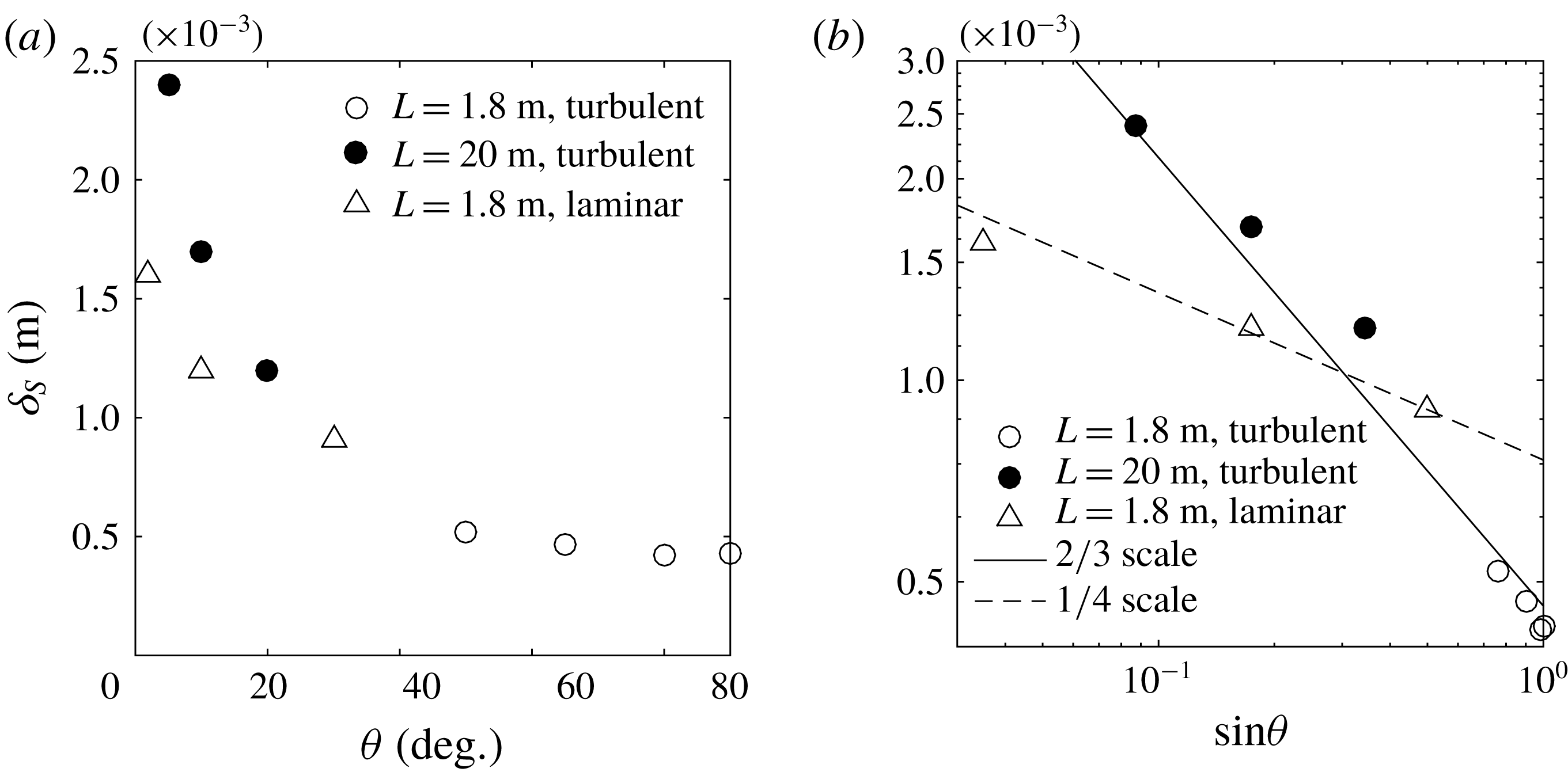
. Both laminar and turbulent ablation rates monotonically increase with the slope angle. The turbulent ablation rates are more sensitive to the ice face inclination than are the laminar rates. The laminar cases show a
 $(\sin \unicode[STIX]{x1D703})^{1/4}$
dependence (3.7), whereas turbulent ablation rates follow a
 $(\sin \unicode[STIX]{x1D703})^{2/3}$
dependence (figure 9
b). Both of these behaviours are predicted by the theoretical scaling in (3.7) and (3.25). In figure 10(a) we plot the thermal boundary layer thickness (
 $\unicode[STIX]{x1D6FF}_{T}$
) as a function of the slope angle, where
 $\unicode[STIX]{x1D6FF}_{T}$
is measured as the temperature e-folding distance from the ice–water interface. The measured boundary layer thickness increases with decreasing slope angle, with trends again depending on whether the boundary layer is laminar or turbulent. The thickness of the thermal boundary layer for laminar flow increases as
 $(\sin \unicode[STIX]{x1D703})^{-1/4}$
(figure 10
b). For turbulent flow the layer thickness is more sensitive to the slope angle and approximately follows
 $(\sin \unicode[STIX]{x1D703})^{-2/3}$
. Both behaviours are again consistent with the theoretical scaling in (3.11) and (3.27). The corresponding thickness of the salinity boundary layer (figure 11) behaves in an identical fashion and is approximately one half of the thermal boundary layer thickness.
Thermal boundary layer thickness
 $\unicode[STIX]{x1D6FF}_{T}$
(m) as a function of (a) slope angle
 $\unicode[STIX]{x1D703}$
and (b)
 $\sin \unicode[STIX]{x1D703}$
(scales are logarithmic). Solid and dotted line show the predicted scaling, (3.11) and (3.27), respectively. Symbols as in figure 9.

Salinity boundary layer thickness
 $\unicode[STIX]{x1D6FF}_{S}$
(m) as function of (a) slope angle
 $\unicode[STIX]{x1D703}$
and (b)
 $\sin \unicode[STIX]{x1D703}$
(scales are logarithmic). Solid and dotted line shows the predicted scaling of (3.4) and (3.23), respectively. Symbols as in figure 9.
(a) Snapshot of slope-normal advective buoyancy flux (sum of mean (
 $U_{\unicode[STIX]{x1D702}}\unicode[STIX]{x1D70C}^{\ast }$
) and turbulent (
 $u_{\unicode[STIX]{x1D702}}^{\prime }\unicode[STIX]{x1D70C}^{\prime }$
) advective fluxes in
 $\text{kg}~\text{s}^{-1}~\text{m}^{-2}$
), for
 $L=1.8~\text{m}$
and
 $\unicode[STIX]{x1D703}=80^{\circ }$
. (b) Absolute value of time- and area-averaged total wall-normal buoyancy flux as a function of
 $\sin \unicode[STIX]{x1D703}$
, where the real values are negative; scales are logarithmic. In (a) the slope-normal distance is enlarged by approximately 10 times relative to the slope-parallel scale in order to show the structure inside the boundary layer. In (b) the dashed line has slope
 $2/3$
. The averaging is over a period
 $\unicode[STIX]{x1D70F}\sim 10\unicode[STIX]{x1D70F}_{b}$
and across the thickness of the boundary layer.

The instantaneous distribution of turbulent kinetic energy,
 $K$
(colour scale in
 $\text{m}^{2}~\text{s}^{-3}$
) in turbulent boundary layers for slope angle (a)
 $\unicode[STIX]{x1D703}=50^{\circ }$
and (b)
 $\unicode[STIX]{x1D703}=90^{\circ }$
for
 $L=1.8~\text{m}$
and (c)
 $\unicode[STIX]{x1D703}=5^{\circ }$
and (d)
 $\unicode[STIX]{x1D703}=20^{\circ }$
for
 $L=20~\text{m}$
. A middle portion of the domain (the actively turbulent region) is shown, and in (c) and (d) the slope-normal distance is enlarged by approximately 10 times relative to the slope-parallel scale in order to more clearly show the turbulent activity in the boundary layer.

The wall-normal advective buoyancy flux (
 $gu_{\unicode[STIX]{x1D702}}\unicode[STIX]{x1D70C}^{\ast }/\unicode[STIX]{x1D70C}_{0}$
) based on wall-normal velocity
 $u_{\unicode[STIX]{x1D702}}$
and density anomaly
 $\unicode[STIX]{x1D70C}^{\ast }$
is shown in figure 12(a). Although the wall-normal buoyancy flux shows significant spatial variability associated with strong turbulent patches, the averaged value is negative. The magnitude of the averaged advective buoyancy flux shows increasing magnitude with the slope angle as
 $(\sin \unicode[STIX]{x1D703})^{2/3}$
(see figure 12
b). The ablation rate is also coupled to the net transport of buoyancy across the boundary layer. Hence the trend in buoyancy flux with slope angle is consistent with the change in ablation rate with slope angle as shown in (3.25). Under the conditions used here, the turbulent advection (
 $g\langle {u_{\unicode[STIX]{x1D702}}}^{\prime }\unicode[STIX]{x1D70C}^{\prime }/\unicode[STIX]{x1D70C}_{0}\rangle$
) accounts for more than
 $80\,\%$
of the total advective buoyancy flux in the wall-normal direction. The scaling (3.25) for transport can be compared with previous experiments for turbulent natural convection beneath a forward facing inclined heated plane (Vliet & Ross Reference Vliet and Ross1975), where uniform heat flux was imposed over the whole plane. In that case, the heat transfer coefficient,
 $Nu$
(the normalised heat transport), varies as the
 $1/4$
power of the flux Grashof number,
 $Gr_{F}^{\ast }$
. This is effectively the
 $1/3$
power of the Grashof number based on the temperature difference
 $\unicode[STIX]{x0394}T$
and modified gravity
 $g^{\ast }=g(\sin \unicode[STIX]{x1D703})^{2}$
(where
 $Gr^{\ast }=g^{\ast }\unicode[STIX]{x1D6FC}\unicode[STIX]{x0394}TL^{3}/\unicode[STIX]{x1D708}^{2}$
and the extra
 $\sin \unicode[STIX]{x1D703}$
dependence is due to stratification). The result therefore suggests the heat transfer coefficient in that thermal convection problem follows
 $Nu\sim (\sin \unicode[STIX]{x1D703})^{2/3}$
, as is observed here for the solutal flux.
The turbulent kinetic energy (
 $K$
), denoted by
 $K=(1/2)u_{i}^{\prime }u_{i}^{\prime }$
with index representing the
 $\unicode[STIX]{x1D702}$
,
 $y$
and
 $\unicode[STIX]{x1D701}$
directions, is the energy associated with the fluctuating motions in the boundary layers. The fluctuating (primed) component
 $u_{i}^{\prime }=u_{i}-U_{i}$
, is calculated using spanwise spatial average
 $U_{i}$
. The turbulent kinetic energy budget can be expressed as
 $$\begin{eqnarray}\displaystyle \frac{\unicode[STIX]{x2202}K}{\unicode[STIX]{x2202}t}+u_{j}\frac{\unicode[STIX]{x2202}K}{\unicode[STIX]{x2202}x_{j}}=P-\unicode[STIX]{x1D700}+B-\frac{\unicode[STIX]{x2202}\unicode[STIX]{x1D6E4}}{\unicode[STIX]{x2202}x_{j}}, & & \displaystyle\end{eqnarray}$$
where
 $P$
is the turbulent shear production
 $$\begin{eqnarray}\displaystyle P=-\overline{u_{i}^{\prime }u_{j}^{\prime }}\frac{\unicode[STIX]{x2202}U_{i}}{\unicode[STIX]{x2202}x_{j}}, & & \displaystyle\end{eqnarray}$$
 $\unicode[STIX]{x1D700}$
is the turbulent dissipation
 $$\begin{eqnarray}\displaystyle \unicode[STIX]{x1D700}=\unicode[STIX]{x1D708}\overline{\frac{\unicode[STIX]{x2202}u_{i}^{\prime }}{\unicode[STIX]{x2202}x_{j}}\frac{\unicode[STIX]{x2202}u_{i}^{\prime }}{\unicode[STIX]{x2202}x_{j}}}, & & \displaystyle\end{eqnarray}$$
 $B$
is the turbulent buoyancy production
 $$\begin{eqnarray}\displaystyle B=-g\overline{\unicode[STIX]{x1D70C}^{\prime }u_{\unicode[STIX]{x1D701}}^{\prime }}\sin \unicode[STIX]{x1D703}+g\overline{\unicode[STIX]{x1D70C}^{\prime }u_{\unicode[STIX]{x1D702}}^{\prime }}\cos \unicode[STIX]{x1D703} & & \displaystyle\end{eqnarray}$$
and the term
 $\unicode[STIX]{x2202}\unicode[STIX]{x1D6E4}/\unicode[STIX]{x2202}x_{j}$
denotes the turbulent advection of
 $K$
,
 $$\begin{eqnarray}\displaystyle \unicode[STIX]{x1D6E4}\equiv p^{\prime }u_{i}^{\prime }+\frac{1}{2}\overline{u_{i}^{\prime }u_{i}^{\prime }u_{j}^{\prime }}-\unicode[STIX]{x1D708}\frac{\unicode[STIX]{x2202}K}{\unicode[STIX]{x2202}x_{j}}, & & \displaystyle\end{eqnarray}$$
containing the pressure transport, turbulent transport and viscous transport.
Snapshot of rates of (a) turbulent shear production,
 $P$
(
 $\text{m}^{2}~\text{s}^{-3}$
), (b) buoyancy production
 $B$
(
 $\text{m}^{2}~\text{s}^{-3}$
) and (c) viscous dissipation,
 $\unicode[STIX]{x1D700}$
(expressed in a logarithmic colour scale) for
 $\unicode[STIX]{x1D703}=90^{\circ }$
in 1.8 m domain.

Snapshot of rates of (a) turbulent shear production
 $P$
(
 $\text{m}^{2}~\text{s}^{-3}$
), (b) buoyancy production
 $B$
(
 $\text{m}^{2}~\text{s}^{-3}$
) and (c) viscous dissipation
 $\unicode[STIX]{x1D700}$
(expressed in logarithmic scale) for
 $\unicode[STIX]{x1D703}=10^{\circ }$
and
 $L=20~\text{m}$
. The slope-normal distance is enlarged by approximately 10 times relative to the slope-parallel scale in order to show the structure inside the boundary layer.

Snapshots of
 $K$
for the shorter and longer domain are shown in figures 13(a), 13(b) and 13(c), 13(d) respectively. For all cases
 $K$
increases in the up-slope direction and the boundary layer thickens. For a given slope length,
 $K$
is larger for the steeper ice faces. For the smaller slope, turbulence develops further along the ice interface (figure 13
c,d).
The instantaneous turbulent shear production rate
 $P$
, buoyancy production rate
 $B$
, and viscous dissipation rate
 $\unicode[STIX]{x1D700}$
are shown in figure 14 for the steepest (
 $\unicode[STIX]{x1D703}=90^{\circ }$
) ice face and in figure 15 for a small slope angle (
 $\unicode[STIX]{x1D703}=10^{\circ }$
). The turbulent dissipation rate is always maximum at the ice face at all distances along the slope. A significant difference in the relative magnitude of turbulent production (compared with other terms in the energy budget) is observed. For the shallower slopes, turbulent shear production is an order of magnitude greater than buoyancy production, whereas for a vertical ice face the shear production is similar to the buoyancy production. The relative contributions of turbulent fluxes in the production of turbulent kinetic energy
 $K$
are plotted in figure 16(b), where the time- and area-averaged
 $K$
, dissipation, shear and buoyancy production are denoted by,
 $\langle K\rangle ,\langle \unicode[STIX]{x1D700}\rangle ,\langle T\rangle$
and
 $\langle B\rangle$
respectively, and are calculated as:
 $$\begin{eqnarray}\displaystyle & \displaystyle \langle K\rangle =\frac{1}{2\unicode[STIX]{x1D70F}A}\int _{A}\int _{\unicode[STIX]{x1D70F}}\overline{u_{i}^{\prime }u_{i}^{\prime }}\,\text{d}t\,\text{d}A, & \displaystyle\end{eqnarray}$$
 $$\begin{eqnarray}\displaystyle & \displaystyle \langle P\rangle =-\frac{1}{\unicode[STIX]{x1D70F}A}\int _{A}\int _{\unicode[STIX]{x1D70F}}\overline{u_{i}^{\prime }u_{j}^{\prime }}\frac{\unicode[STIX]{x2202}U_{i}}{\unicode[STIX]{x2202}x_{j}}\,\text{d}t\,\text{d}A, & \displaystyle\end{eqnarray}$$
 $$\begin{eqnarray}\displaystyle & \displaystyle \langle \unicode[STIX]{x1D700}\rangle =\frac{1}{\unicode[STIX]{x1D70F}A}\int _{A}\int _{\unicode[STIX]{x1D70F}}\unicode[STIX]{x1D708}\overline{\frac{\unicode[STIX]{x2202}u_{i}^{\prime }}{\unicode[STIX]{x2202}x_{j}}\frac{\unicode[STIX]{x2202}u_{i}^{\prime }}{\unicode[STIX]{x2202}x_{j}}}\,\text{d}t\,\text{d}A & \displaystyle\end{eqnarray}$$
and
 $$\begin{eqnarray}\displaystyle \langle B\rangle =\frac{1}{\unicode[STIX]{x1D70F}A}\int _{A}\int _{\unicode[STIX]{x1D70F}}g(-\overline{\unicode[STIX]{x1D70C}^{\prime }u_{\unicode[STIX]{x1D701}}^{\prime }}\sin \unicode[STIX]{x1D703}+\overline{\unicode[STIX]{x1D70C}^{\prime }u_{\unicode[STIX]{x1D702}}^{\prime }}\cos \unicode[STIX]{x1D703})\,\text{d}t\,\text{d}A. & & \displaystyle\end{eqnarray}$$
The averaging time window is
 $\unicode[STIX]{x1D70F}\sim 10\unicode[STIX]{x1D70F}_{b}$
and
 $A$
is the area (in the
 $\unicode[STIX]{x1D701}$
and
 $\unicode[STIX]{x1D702}$
plane) containing the boundary layer in the upper half of the domain length, where the boundary layer is fully turbulent. For steep slopes (figure 16
a)
 $K$
is large and the value of
 $\langle B\rangle$
is comparable or slightly larger than that of
 $\langle P\rangle$
. For small slopes (
 $\unicode[STIX]{x1D703}\leqslant 20^{\circ }$
)
 $\langle P\rangle$
dominates over
 $\langle B\rangle$
.
The production of turbulence, either by velocity shear or buoyancy, is significantly influenced by density stratification and gravity at both limits of ice face inclination. When the slope is steep (
 $\unicode[STIX]{x1D703}\geqslant 80^{\circ }$
), turbulent buoyancy flux (predominantly produced in the plume) is less impacted by the weak vertical (stable) buoyancy gradient produced by the solutal boundary layer. In contrast, the buoyancy production for small angles is reduced significantly by two mechanisms. First there is a large reduction in the buoyancy force in the up-slope direction (
 $g\sin \unicode[STIX]{x1D703}$
), which produces the slope-parallel components of
 $\langle B\rangle$
. In addition the development of stable stratification under the sloping ice face causes the turbulent advection in the wall-normal direction to decrease, resulting in smaller buoyancy production. For small slopes the mean shear is large enough to produce turbulence despite the density stratification (while convection is inhibited) and, as a result, the turbulent shear production becomes the dominant mechanism for maintaining turbulence in the boundary layer.
Normalised time- and area-averaged turbulent statistics as function of slope angle; (a) turbulent kinetic energy
 $\langle K\rangle$
is normalised by characteristic velocity scale
 $U_{c}\sim (g\unicode[STIX]{x1D6FD}\unicode[STIX]{x0394}SL)^{1/2}$
, (b) turbulent dissipation
 $\langle \unicode[STIX]{x1D700}\rangle$
, buoyancy production
 $\langle B\rangle$
, and turbulent shear production
 $\langle P\rangle$
, for 1.8 m domain (filled symbols) and for 20 m domain (open symbols) normalised using the respective domain length
 $L$
and velocity scale
 $U_{c}$
.

5 Discussion and conclusions
This paper presents the first DNS of ice dissolution due to convection under a sloping ice face. We have simulated fully turbulent flow at geophysically relevant slopes (
 $\unicode[STIX]{x1D703}\leqslant 40^{\circ }$
) at temperature and salinities relevant to Antarctic conditions. The typical Grashof number based on the vertical height of the ice–seawater interface is of the order of
 $Gr^{\bot }\sim 10^{17}{-}10^{19}$
, for heights in the range 200–800 m. Although this range is not achievable using DNS with present computational capacity, we have chosen large Grashof numbers (
 $Gr^{\bot }\sim 10^{10}{-}10^{11}$
), which are well above the critical
 $Gr_{c}^{\bot }\sim 10^{9}$
for the transition to turbulent convection on a vertical heated wall. The solutions confirm that these conditions ensure a steady but turbulent mean flow. The boundary layer flow changes significantly with the slope. For steep angles a narrow up-slope flow of relatively fresh buoyant water develops close to the wall. For small slope angles (
 $\unicode[STIX]{x1D703}<20^{\circ }$
), the buoyant up-slope flow is relatively weak due to the reduction of buoyancy force in the along-slope direction. However, the solutions at large Grashof numbers again show a turbulent flow.
Boundary layer properties and ablation rates are dependent on whether the boundary layer is laminar or turbulent. Both the thermal and solutal boundary layer thicknesses increase with decreasing slope angle, resulting in the reduction of heat and salt transport to the interface and consequent reduction of the ablation rate. In the laminar case the ablation rate decreases with along-slope distance as
 $\unicode[STIX]{x1D701}^{-1/4}$
, consistent with theoretical scaling. In contrast the turbulent cases have ablation rates that are nearly uniform along the slope, as previously found for vertical ice faces (Kerr & McConnochie Reference Kerr and Mcconnochie2015; Gayen et al.
Reference Gayen, Griffiths and Kerr2016). We hypothesise that for domain lengths larger than those achieved in the present DNS, and having a Grashof number greater than the critical value, dissolution rate will be given by the asymptotic dynamics of turbulent boundary layer flow, and the present results can be extrapolated to geophysical scales following the scaling presented here. In that case, for a purely convective boundary layer, the ablation of ice faces into the ocean will follow
 $V\simeq (\sin \unicode[STIX]{x1D703})^{2/3}$
. This leads to a simple modification of the previously derived dependence of melt rate on the driving temperature difference (Kerr & McConnochie Reference Kerr and Mcconnochie2015; Gayen et al.
Reference Gayen, Griffiths and Kerr2016), now taking account of the interface slope as:
 $$\begin{eqnarray}\displaystyle V\simeq 8.98\times (\unicode[STIX]{x0394}T_{L})^{4/3}(\sin \unicode[STIX]{x1D703})^{2/3}\;\text{m}~\text{yr}^{-1}. & & \displaystyle\end{eqnarray}$$
An alternative scaling reported by Magorrian & Wells (Reference Magorrian and Wells2016) is based on a buoyant plume model and gives a greater sensitivity of melt rates on
 $\unicode[STIX]{x1D703}$
for small slopes (
 $V\sim (\sin \unicode[STIX]{x1D703})^{3/2}$
) and an inverse dependence on slope angle (
 $V\sim 1/\sin \unicode[STIX]{x1D703}$
) for near-vertical interfaces. Those trends are not reflected in the present DNS results. The discrepancy may result from a different regime of the convective boundary layer. The model of Jenkins (Reference Jenkins1991) and Magorrian & Wells (Reference Magorrian and Wells2016) assumes a regime in which the thickness of the laminar sub-layer near the ice face is controlled primarily by shear instability (Grossmann & Lohse Reference Grossmann and Lohse2000; Wells & Worster Reference Wells and Worster2008) rather than convective instability as found here. The transition to this shear-dominated regime at steep slopes for saline convection was predicted to occur at
 $Gr\sim 10^{20}$
, which occurs for vertical ice heights of hundreds of metres. The present study uses heights/domain lengths where the boundary layer on near-vertical interfaces remains controlled by turbulent convection. Hence it remains to be demonstrated whether the transition can occur. Further discussion of transition between these two regimes can be found in McConnochie & Kerr (Reference McConnochie and Kerr2017b
).
The turbulent kinetic energy budget shows the presence of statistically steady turbulence in the simulated flow fields for slope angles as small as,
 $\unicode[STIX]{x1D703}=5^{\circ }$
. For near-vertical slopes (
 $\unicode[STIX]{x1D703}>80^{\circ }$
) contributions to turbulent kinetic energy from shear production and buoyancy flux are comparable, with a slightly greater contribution from the buoyancy flux. For small slopes the production of turbulent kinetic energy by buoyancy fluxes is significantly smaller than the turbulent shear production. This potentially implies that the shear associated with large-scale ambient geostrophic currents and barotropic tides in the ocean is more likely to contribute to the turbulent transport at the ice face and enhance the melt rate for small slopes.
The present study has focused on the effect of ice face slope on melting that is driven by natural convection. The natural convection on its own can be viewed as a base, or reference, case given that natural convection will always be present irrespective of the magnitude and influence of shear associated with ambient geostrophic currents, internal waves or sub-glacial discharge plumes. The next step will be to include ambient stratification (McConnochie & Kerr Reference McConnochie and Kerr2016b ), subglacial discharge of fresh water (McConnochie & Kerr Reference McConnochie and Kerr2017a ) and ambient shear.
Acknowledgements
Computations were carried out using the Australian National Computational Infrastructure, through the National Computational Merit Allocation Scheme supported by the Australian Government. This work was supported by Australian Research Council grants DP120102772 and DP120102744. B.G. was supported by ARC DECRA Fellowship DE140100089 and an Australian Antarctic Division RJL Hawk Fellowship to B.G. We are also grateful to the reviewers who provided valuable suggestions throughout the review process.



