1. Background

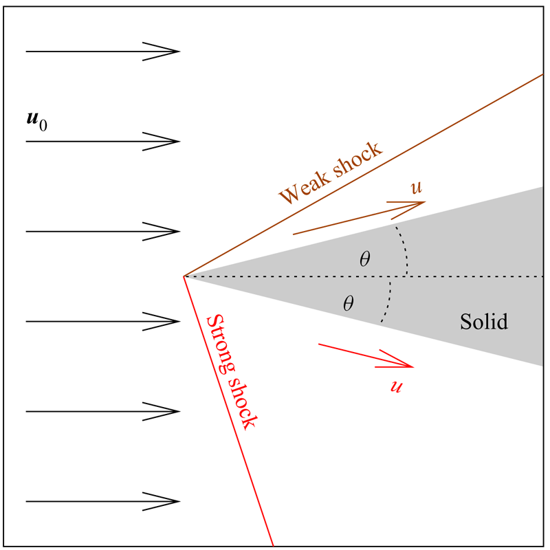
Given a fixed state on the upstream side of an oblique steady shock, the shock polar (figure 1) is the curve of all possible downstream velocities that can be generated by varying the angle of the shock. Polars are useful for flow onto sharp narrow wedges (or blunt ones seen at a distance), which have shocks attached to the leading edge (figure 2). The shock must turn the upstream velocity $\boldsymbol {{ u}}_0$ by a given angle $\theta$ to produce a downstream velocity $\boldsymbol {{ u}}$ parallel to the solid surface. For $\theta$ less than the critical angle the polar (figure 1) shows two shock solutions; the weaker one is commonly observed.

Figure 1.

Shock polar ($f=5$ polytropic, $M_0=2.5$), symmetric across $\boldsymbol {{ u}}_0=(1,0)$ axis.

Figure 2.

Supersonic flow onto wedge (strong shock usually not observed).

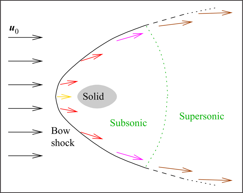
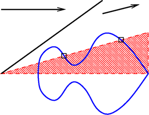
In bow shocks ahead of a blunt body (figure 3) all velocities along the polar are realized, with a normal shock on the symmetry axis and the limit of vanishing shocks at infinity.

Figure 3.

Bow shock ahead of a blunt body in supersonic flow (subsonic regions need not enclose the body).

Shock polars are also important for many other flow patterns with oblique shocks, for example interaction with expansion fans, slip lines and density discontinuities, incident shocks interacting with each other or with solid surfaces, in regular or Mach reflections, etc. (von Neumann Reference von Neumann1943; Ben-Dor Reference Ben-Dor1992; Vasilev & Kraiko Reference Vasilev and Kraiko1999; Hunter & Tesdall Reference Hunter and Tesdall2002; Skews & Ashworth Reference Skews and Ashworth2005; Elling & Liu Reference Elling and Liu2008; Elling Reference Elling2010, Reference Elling2012).

The shock polar depends not only on the upstream state, in particular on its Mach number $M_0$, but also on the fluid. We call a gas ideal (or sometimes ‘perfect’ or ‘thermally perfect’) if the pressure $p$, volume per mass $V=1/\varrho$ and temperature $T$ are related by $p V/ T= R_s$ with constant $R_s$. Then internal energy per mass $e$ is a function of temperature alone. If the function is linear, $e=\frac 12 \,f\kern0.7pt R_s T$ with constant $f$, then we call the gas polytropic (or sometimes ‘calorically perfect’).

For a polytropic gas, exact polar formulas have been known for a long time (Meyer Reference Meyer1908; Busemann Reference Busemann1931; Courant & Friedrichs Reference Courant and Friedrichs1948): for $\boldsymbol {{ u}}_0$ rotated and scaled to $( u^x_0, u^y_0)=(1,0)$,

(1.1a–c)\begin{equation} u^y ={\pm} (1- u^x) \sqrt{\frac{ u^x- u^x_{nor}}{ u^x_{max}- u^x}} ,\quad u^x_{nor} = \frac{1+ f\kern0.7pt M_0^{{-}2}}{ f+1} ,\quad u^x_{max} = 1 + \frac{ f\kern0.7pt M_0^{{-}2}}{ f+1}, \end{equation}

where $u^x_{nor}$ is $u^x$ for a normal shock. Using this formula, it is easily checked that the ‘$+$’ branch of $u^y$ is a strictly concave function of $u^x$ between $u^x_{nor}$ and $u^x_0$, so that the upper half of the polar has exactly one local maximum of the velocity angle, a critical-type shock where the polar is tangent to the $\theta$ ray.

No solutions exist for larger $\theta$; for smaller, there is a weak-type shock where the polar crosses the ray non-tangentially from below to above (as we pass from vanishing to normal shock, see figure 1), with an opposite crossing at the strong-type shock.

Although strong-type reflections can be generated by careful adjustment of the parameters, they are not stable under parameter changes (Teshukov Reference Teshukov1989; Elling & Liu Reference Elling and Liu2006; Elling Reference Elling2009b). More precisely, for problems posed so that their linearization around a weak shock background has unique solutions, the same problem linearized around a strong shock requires one scalar constraint satisfied for existence (Elling Reference Elling2009a). For this reason, the observed shocks are mostly weak type, and for polytropic polars there is only one such shock.

2. Motivation

Polytropic equations of state (e.o.s.) are a rather loose approximation for the most important gases. Define $f=2( c_p/ R_s-1)$ with specific heat at constant pressure $c_p=(\partial h/\partial T)_{ p}$, where subscript $p$ indicates the $p$ coordinate is held constant for taking the $T$ partial derivative; $h= e+ p V$ is enthalpy per mass. A polytropic flow is characterized by constant $f$; $f=3$ is used for monatomic gases, $f=5$ for diatomic ones like oxygen.

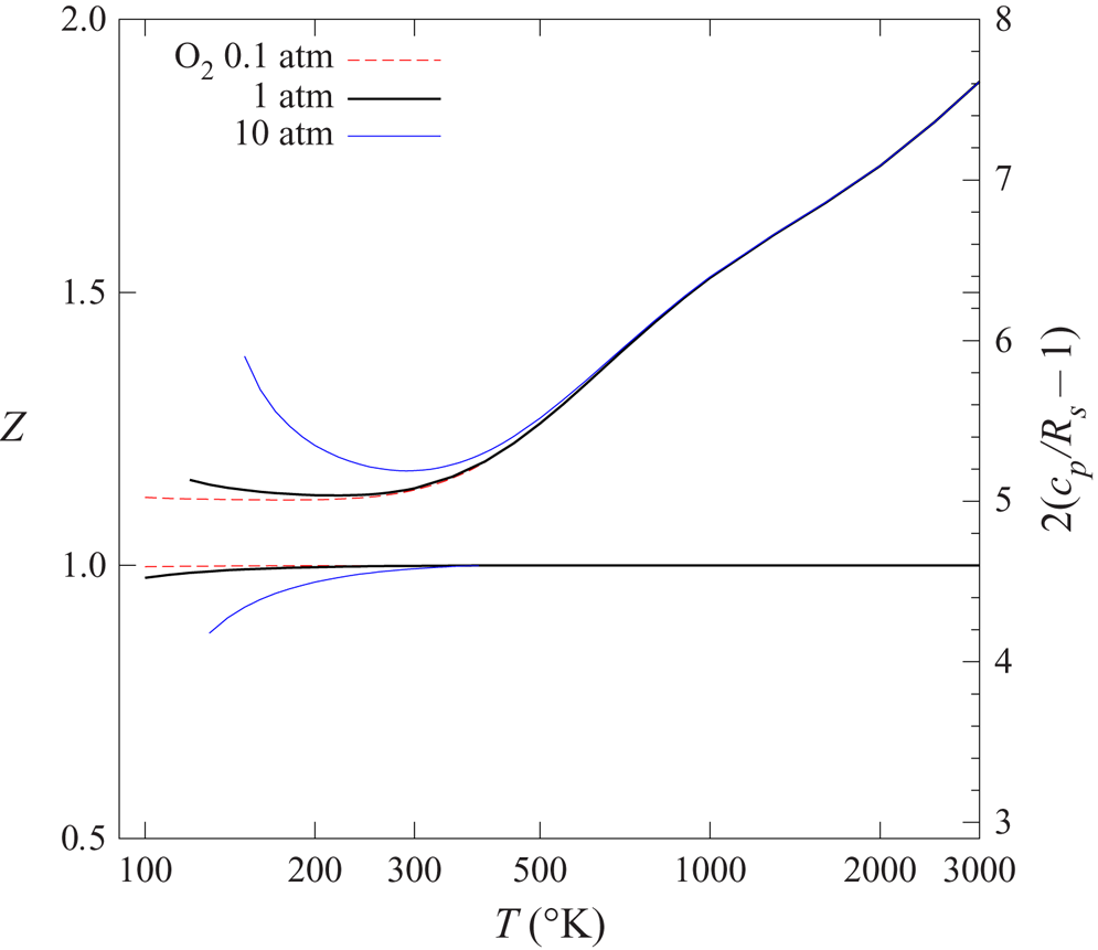
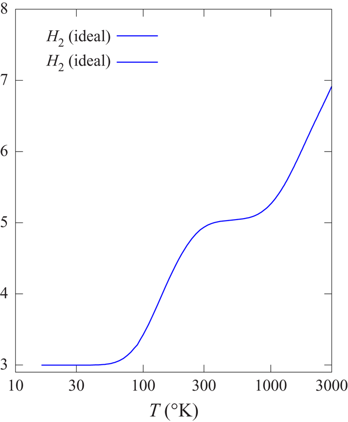
For oxygen at atmospheric pressure, $f$ stays between 5.0 and 5.1 up to room temperature (see figure 4), but crosses above 5.4 already at 500 Kelvin. Similar observations can be made for most other multiatomic gases, including the important cases of nitrogen/air, carbon dioxide and hydrogen (cf. figure 5, see also Woolley, Scott & Brickwedde (Reference Woolley, Scott and Brickwedde1948, figure 3) for experimental/modelled $c_p$ at high temperature).

Figure 4.

Value of $Z$ (lower curves; see (2.1)) and $2( c_p/ R_s-1)$ (upper) for molecular oxygen (Woolley Reference Woolley1953); $Z\approx 1$ indicates ideal behaviour, constant $2( c_p/ R_s-1)$ polytropic.

Figure 5.

Value of $2( c_p/ R_s-1)$ for molecular hydrogen (normal); rotational quanta are large enough for decrease to $3$ at low $T$ (Woolley et al. Reference Woolley, Scott and Brickwedde1948).

Clearly $f$ is near constant only over narrow temperature ranges, which are easily exceeded by many applications, e.g. high-supersonic flight, flow after combustion, ramjet/scramjet inlets or atmospheric entry (Boyd, Candler & Levin Reference Boyd, Candler and Levin1995; Gnoffo Reference Gnoffo1999).

In classical mechanics $f$ represents degrees of freedom per gas particle, three for linear motion of hard-sphere models of atoms, another two for visible rotation axes of rigid-dumbbell models of diatomic molecules, etc., with equal average energy $\frac 12 k_B T$ in each degree (Boltzmann equipartition), and a continuum of possible energies. But energy levels are discrete in quantum-mechanical reality. There, constant integer $f$ are only suitable when the quanta are either much larger than temperature, so that most molecules are in the ground state (degree of freedom effectively absent, as for bond-axis vibration of oxygen or nitrogen at room temperature), or much smaller so that the energy levels resemble a continuum (rotational quanta for most gases, with hydrogen a notable exception, cf. figure 5). At intermediate temperatures, $f$ necessarily rises through fractional values.

Beyond polytropic, the next more accurate model is a non-polytropic ideal gas. But there, we can find examples of $e= e( T)$ that have shock polars with multiple velocity angle maxima (see figure 6, § 5), so that some turning angles $\theta$ have four or more theoretical solutions. In order of increasing strength, the solutions alternate between strong and weak type. Even if we exclude the strong-type half on stability grounds, multiple weak-type shocks remain.

Figure 6.

A $M_0=1.225$ ideal gas polar with multiple velocity angle maxima (b), caused by a cubic spline increase (a) in $e/ T$.

Multiple solutions are a major concern for applications. Regular and Mach reflections are already suspected to coexist for some parameters, with steady flow switching between them in unsteady hysteresis (Hornung, Oertel & Sandeman Reference Hornung, Oertel and Sandeman1979; Chpoun et al. Reference Chpoun, Passerel, Li and Ben-Dor1995; Laguarda et al. Reference Laguarda, Hickel, Schrijer and van Oudsheusden2020). Multiple solutions can cause numerics or experiments to overlook flows that occur in reality. Such mispredictions can have significant effects, persistent such as incorrect stress or heat flow estimates, or spontaneous such as engine unstart, possibly hard to diagnose even in hindsight. Even when all steady flows are detected in advance, spontaneous and unpredictable transitions between them are unacceptable in many applications (consider sudden flow changes or vibrations in engines operating close to their stress/temperature limits).

One route is to look for reasons why one of several weak-type shocks should be preferred. However, considering that the change of $e( T)$ in figure 6 is unusually sharp, we should first look for simple conditions excluding the possibility of multiple weak-type solutions altogether.

They can easily be excluded for any concrete $e( T)$ and $T_0, p_0, M_0$ by numerical calculations. Numerics are commonly used to compute polars or Hugoniot curves in complex non-ideal cases (e.g. Short & Quirk Reference Short and Quirk2018a, figures 6 and 7; Alferez & Touber Reference Alferez and Touber2017, figure 1; Lieberthal, Stewart & Hernandez Reference Lieberthal, Stewart and Hernandez2017, § 6.1; Huete & Vera Reference Huete and Vera2019, figure 1); in such complex cases there is little hope of finding simple analytic formulas for the shock polar. However, numerical plotting has to be repeated for each fluid and each upstream state. Even for an ideal gas, the possible equations of state form an infinite-dimensional parameter space; trying to cover it numerically is slow and error prone.

Nor is it necessary: for ideal gas we show that the allowed $e( T)$ can be characterized precisely by the familiar condition of a convex equation of state (also expressed as the ‘positive fundamental derivative’), namely positive $(\partial ^2 p/\partial V^2)_{ s}$. This is satisfactory since only a few materials are known or claimed to violate the condition, in regions far from ideal behaviour. (Besides, whenever it is violated compressive shocks may be non-admissible, so that the correct flow turning by a particular angle $\theta$ may well be a composite of several waves rather than a single shock (see Vimercati, Kluwick & Guardone Reference Vimercati, Kluwick and Guardone2018, figure 1).) Our other conditions are standard: positive heat capacity, positive speed of sound, etc. (see § 6).

Idealness is a close approximation over large temperature ranges. This is quantified using the compressibility factor

(2.1)\begin{equation} Z = \frac{ p V}{ R_s T}, \end{equation}

with $Z$ near constant considered ideal behaviour. For oxygen at atmospheric pressure $Z\approx 1$ from $100\,\textrm {K}$ to well over $3000\,\textrm {K}$ (figure 4). (As in Woolley (Reference Woolley1953) we use $R_s= R_u/M$, where $M$ is molar mass at a reference state such as standard conditions; as temperature increases $Z$ rises through dissociation of molecular to atomic oxygen from $1$ to a new plateau of $2$, which is again considered ideal.) For most gases, the low end of the ideal temperature range is due to increasing density permitting significant intermolecular forces, usually near the boiling/sublimation point (${\approx }90\,\textrm {K}$ for oxygen at 1 atm) except at high pressures. The high end is usually due to dissociation or ionization, e.g. $\text {O}_\text {2}\rightleftharpoons 2\text {O}$ between $3000$ and $4000\,\textrm {K}$, higher for nitrogen. However, a fully dissociated neutral gas is ideal again. ($p= R_u T n$, with $n$ moles per volume, is also commonly called the ‘ideal gas law’; for chemically reacting mixtures it is not equivalent to $p= R_s T\varrho$. Some of the literature objects to calling dissociation a ‘non-ideal’ effect.)

In any case, the results of this article confirm benign behaviour of shock polars for a much wider range of temperatures.

In § 10 we first argue our results cannot hold for general (non-ideal) gas assuming only a convex e.o.s. So we focus on important special cases like dissociation, e.g. of molecular into atomic oxygen, important in atmospheric entry (Boyd et al. Reference Boyd, Candler and Levin1995; Gnoffo Reference Gnoffo1999). Our numerical experiments suggest a positive fundamental derivative and that the uniqueness of critical-type shocks still holds, except at unrealistically low pressures.

Dissociation is a special case of reversible chemical reactions. In practice, irreversible reactions are important, e.g. in fuel-oxidizer mixtures passing through an engine. But there, cases of non-uniqueness can be found easily, even for normal steady shocks, with one solution a detonation, the other solution a weaker shock that does not ignite the mixture.

3. Outline of the ideal polar argument

Since the precise argument is long, we first outline the core idea by an informal argument based on mass flux. The argument gives a clear intuitive idea why critical-type shocks are generally subsonic.

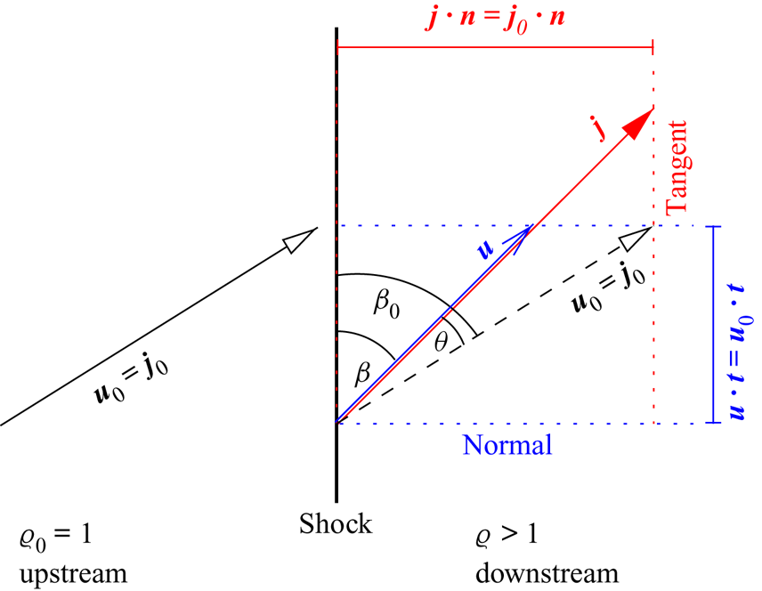
A good coordinate-free representation of the turning angle $\theta$ is to represent it as

(3.1)\begin{equation} \theta = \beta_0-\beta, \end{equation}

where (see figures 7 and 8) subscript $0$ indicates the upstream side, no subscript means downstream and $\beta ,\beta _0$ are the angles between shock and velocity $\boldsymbol {{ u}}$ or $\boldsymbol {{ u}}_0$; the length of $\boldsymbol {{ u}}$ is $u$, etc. Tangential velocity $u^t$ is continuous across the shock, as is the normal part $j^n$ of mass flux $\boldsymbol {j}=\varrho \boldsymbol {{ u}}$, so the formulas

(3.2)\begin{equation} \beta = \arccos\frac{ u^t}{ u} = \arcsin\frac{ j^n}{ j} \end{equation}

are especially convenient since the only ‘unknowns’ in $\theta$ involving the thermodynamics are the downstream speed $u$ and mass flux $j$, the rest are purely geometric from $\beta _0, j_0, u_0$.

Figure 7.

Across shocks, the normal mass flux $\boldsymbol {j}\boldsymbol {\cdot }\boldsymbol {n}$ and tangential velocity $\boldsymbol {{ u}}\boldsymbol {\cdot }\boldsymbol {t}$ are continuous ($\varrho _0=1$ scaling in this figure for clarity).

Figure 8.

With $\theta$ and $\boldsymbol {{ u}}_0=\boldsymbol {j}_0$ held fixed, increasing $\beta _0$ decreases $\boldsymbol {{ u}},\boldsymbol {j}$ ($\varrho _0=1$ in this figure for clarity).

The upper half of the shock polar (figure 1) is the curve of $\boldsymbol {{ u}}$ resulting from increasing $\beta _0$ from the Mach angle $\arcsin (1/ M_0)$ (vanishing shock) to $90^\circ$ (normal shock). At a critical-type shock by definition $\theta$ stagnates; holding $\theta$ and $\boldsymbol {{ u}}_0,\boldsymbol {j}_0$ fixed while increasing $\beta _0$ (see figure 8) decreases both $u$ and $j$.

Immediately, a classical observation of fluid dynamics comes to mind (figure 9): along streamlines, decreasing speed $u$ will decrease mass flux $j$ if and only if the flow is subsonic. This explains clearly why the critical-type shocks are generally on the subsonic part of the polar. The classical result assumes constant per-mass total enthalpy $H$ (true for shocks) and constant entropy $s$ (almost true for small shock strength).

Figure 9.

Mass flux as a function of speed at constant entropy and total enthalpy.

The change of mass flux with speed is quantified by the well-known formula

(3.3)\begin{equation} \frac{\delta\ln j}{\delta\ln u} = 1- M^2. \end{equation}

This suggests how to show the uniqueness of critical-type shocks: downstream Mach number $M$ is usually decreasing from vanishing to normal (all ‘decreases’ and ‘increases’ are in the ‘strict’ sense). Then, the right-hand side of (3.3) would be increasing. So it cannot equal more than once the left-hand side, which is decreasing when specialized to critical-type shocks. The last property is less obvious and requires a detailed calculation, given around (9.7).

This is probably as simple as informal arguments can be made, but clearly there are many loose ends. In the following sections, we will carefully fill in every detail and impose missing assumptions.

4. Shock relations

Let $\boldsymbol {n}$ be a unit normal to the shock, $\varDelta {a}=a-a_0$ be the jump of some quantity $a$ from upstream to downstream, with $\bar {a}=\frac 12(a+a_0)$ the average of both sides. Conservation of mass, momentum and energy for a steady straight shock gives

(4.1)\begin{gather} 0 = \varDelta{ j^n}, \end{gather}

(4.2)\begin{gather}0 = \varDelta\left(\,j^n\boldsymbol{{ u}}\right)+\varDelta\left(p\boldsymbol{n}\right), \end{gather}

(4.3)\begin{gather}0 = \varDelta\left(\,j^n\left( e+\frac{|\boldsymbol{{ u}}|^2}{2}\right)\right)+\varDelta\left( p u^n\right). \end{gather}

Second law of thermodynamics (entropy inequality)

(4.4)\begin{equation} 0 \leq \varDelta\left(\,j^n s\right). \end{equation}

Tangential part of momentum conservation (4.2)

(4.5)\begin{equation} 0 = \varDelta\left(\,j^n u^t\right) \overset{\varDelta{ j^n}=0}= j^n \varDelta{ u^t}, \end{equation}

for shocks $j^n\neq 0$ so that

(4.6)\begin{equation} \varDelta{ u^t}=0 , \end{equation}

so $\varDelta {\boldsymbol {{ u}}}$ is normal to the shock. On the other hand, $\varDelta {\boldsymbol {j}}$ is tangential to the shock, by mass conservation (4.1). We orient shock normals so that $j^n>0$, then the entropy inequality (4.4) reduces to

(4.7)\begin{equation} 0 \leq \varDelta{ s}. \end{equation}

Normal part of momentum conservation (4.2)

(4.8)\begin{align} 0 &= j^n\varDelta{\mathord{\overbrace{\mathop{ u^n}}^{= V\varrho u^n= V j^n}}}+\varDelta{ p} \end{align}

(4.9)\begin{align} &= (\,j^n)^2\varDelta{ V}+\varDelta{ p} \quad\Rightarrow\quad \frac{\varDelta{ p}}{-\varDelta{ V}} = (\,j^n)^2 . \end{align}

From this we can also derive the useful

(4.10) \begin{equation} |\varDelta{\boldsymbol{{ u}}}|^2 \overset{\varDelta{ u^t}=0}= (\varDelta{ u^n})^2 = (\varDelta( V\mathord{\underbrace{\mathop{\varrho u^n}}_{=j^n}}))^2 = (\,j^n\varDelta{ V})^2 \overset{(4.9)}={-}\varDelta{ V}\varDelta{ p}. \end{equation}

Using that $\varDelta {\boldsymbol {{ u}}}$ is a shock normal we may obtain a unit normal $\boldsymbol {n}=\varDelta {\boldsymbol {{ u}}}/|\varDelta {\boldsymbol {{ u}}}|$, so

(4.11)\begin{equation} - \varDelta{ p} \overset{(4.8)}= j^n_0 \varDelta{ u^n} = \varrho_0\boldsymbol{{ u}}_0\boldsymbol{\cdot}\boldsymbol{n} \varDelta{\boldsymbol{{ u}}}\boldsymbol{\cdot}\boldsymbol{n} = \varrho_0\boldsymbol{{ u}}_0\boldsymbol{\cdot}\varDelta{\boldsymbol{{ u}}} , \end{equation}

so if the coordinates are chosen to let $\boldsymbol {{ u}}_0$ point horizontal right, then

(4.12)\begin{equation} p = p_0 + \varrho_0 u_0 ( u_0- u^x) . \end{equation}

Hence, pressure can serve as a horizontal coordinate in the $\boldsymbol {{ u}}$ shock polar plane.

For the energy, in (4.3) we use $p u^n= p V\varrho u^n$ to get

(4.13) \begin{equation} 0 = j^n\varDelta\bigg(\mathord{\mathop{\underbrace{\mathord{\overbrace{\mathop{ p V+ e}}^{= h}}+\frac{|\boldsymbol{{ u}}|^2}{2}}}_{=H}}\bigg) \quad\Rightarrow\quad \varDelta{ H} = 0, \end{equation}

with $H$ the total enthalpy per mass. The shock relations can be reduced further to a single scalar relation: applying $\varDelta \left (a^2\right )=2\bar {a}\varDelta {a}$ to $a= V$,

(4.14)\begin{align} 0 &\overset{(4.13)}{\underset{\varDelta{ u^t}=0}=} \varDelta{ h}+\varDelta\left(\frac{ V^2(\varrho u^n)^2}{2}\right) = \varDelta{ h}+(\,j^n)^2\varDelta\left(\frac{ V^2}{2}\right) \end{align}

(4.15)\begin{align} &= \varDelta{ h} + (\,j^n)^2 \bar{ V} \varDelta{ V} \overset{(4.9)}= \varDelta{ h} - \bar{ V} \varDelta{ p}. \end{align}

This Hugoniot relation involves no (macroscopic) velocities, only thermodynamic quantities. Using $h= e+ p V$ and applying $\varDelta \left (ab\right )=\bar {a}\varDelta {b}+\bar {b}\varDelta {a}$ to $a= p$, $b= V$ shows

(4.16)\begin{equation} 0 = \varDelta{ e} + \bar{ p}\varDelta{ V}, \end{equation}

a common alternate form.

5. Ideal polar

Until § 10.2 we choose units so that $R_s=1$, to simplify calculations. The resulting ideal gas law $V= T/ p$ can be used in the Hugoniot relation (4.16)

(5.1)\begin{equation} 0 = 2\varDelta{ e} + ( p+ p_0)\varDelta{\frac{ T}{ p}}, \end{equation}

this is essentially a quadratic equation for $p$, with solution

(5.2)\begin{equation} \frac{ p}{ p_0} = \frac{\varDelta\left( e+ T/2\right)}{ T_0} + \sqrt{\left(\frac{\varDelta\left( e+ T/2\right)}{ T_0}\right)^2+\frac{ T}{ T_0}} , \end{equation}

where we may ignore the $-\sqrt {\cdot }$ second solution (assuming positive temperatures and pressures). From this we also see

(5.3)\begin{equation} \frac{ V_0}{ V} = \frac{ p}{ p_0} \frac{ T_0}{ T} = \frac{\varDelta\left( e+ T/2\right)}{ T} + \sqrt{\left(\frac{\varDelta\left( e+ T/2\right)}{ T}\right)^2+\frac{ T_0}{ T}} . \end{equation}

As noted in (4.11), there is a linear relationship between $\varDelta { p}$ and $\varDelta { u^x}$, if we rotate $\boldsymbol {{ u}}_0$ to be horizontal pointing right, and having obtained $p$ and $V$, we can use (4.10) $|\varDelta {\boldsymbol {{ u}}}|^2=\varDelta { p}\varDelta \left (- V\right )$ and then

(5.4)\begin{equation} u^y=\varDelta{ u^y}={\pm}\sqrt{|\varDelta{\boldsymbol{{ u}}}|^2-|\varDelta{ u^x}|^2} \end{equation}

to calculate all of $\boldsymbol {{ u}}$. So the steps from (5.2) provide a semi-explicit formula for the shock polar, with $T$ as parameter instead of $u^x$. Unlike the polytropic case, there is no explicit formula for $T$ as a function of $u^x$, except perhaps for special choices of $e= e( T)$.

Although some of our results can be obtained directly from (5.2), etc., this would be cumbersome, since taking derivatives quickly produces unwieldy expressions whose components do not have an obvious physical meaning. But some quick insights are already possible.

Figure 6 shows an example with an artificial $e( T)$ so that $2 e/ R_s T$ increases from 3 to 5 over some temperature interval. The corresponding shock polar is non-convex, with a dent sufficiently strong that some velocity turning angles $\theta$ permit four rather than two solutions. By adding more intervals of increase more dents could be created, allowing any number of solutions.

In physical fluids, the increase is generally not as sharp as in figure 6(a) (cf. figure 5). We will find that for an ideal gas the increase that permits more than two solutions is characterized precisely by the familiar condition of a convex equation of state.

6. Assumptions

6.1. General gas

We consider fluid in thermal equilibrium described by an e.o.s.

(6.1)\begin{equation} e = e( V, s), \end{equation}

with $e$ the internal energy per mass, $V=1/\varrho$ the volume per mass and $s$ the entropy per mass. We assume $e$ is differentiable as often as needed for our purposes. As always

(6.2)\begin{equation} \textrm{d} e = T \,\textrm{d} s - p \,\textrm{d} V , \end{equation}

where $p$ is pressure and $T$ is temperature. Equivalently,

(6.3)\begin{equation} \textrm{d} h = T\,\textrm{d} s + V\,\textrm{d} p \end{equation}

for enthalpy per mass $h= e+ p V$.

Here, $e$ has ‘standard’ coordinates $V, s$, and for $h$ they are $p, s$. Subscript notation $e_ s$ indicates partial derivatives with the other standard coordinate held fixed (e.g. $(\partial e/\partial s)_{ V}$, not $(\partial e/\partial s)_{ p}$).

We make the following assumptions:

1. (i) $T= e_ s>0$ and $p=- e_ V>0$.

2. (ii) Thermodynamic stability: the matrix $e''$ of second derivatives is positive definite. That is equivalent (e.g. Landau & Lifshitz Reference Landau and Lifshitz1980, p. 64) to the three conditions

   (6.4)\begin{equation} c^2 = \left(\frac{\partial p}{\partial\varrho}\right)_{ s} ={-} V^2 \left(\frac{\partial p}{\partial V}\right)_{ s} = V^2 e^{}_{ V V} > 0, \end{equation}
   so that the sound speed $c$ is well defined and positive, and
   (6.5)\begin{equation} c_v = \left(\frac{\partial e}{\partial T}\right)_{ V} = \left.\left(\frac{\partial e}{\partial s}\right)_{ V} \right/ \left(\frac{\partial T}{\partial s}\right)_{ V} = e^{}_ s / e^{}_{ s s} > 0, \end{equation}
   and finally
   (6.6)\begin{equation} c_p=\left(\frac{\partial h}{\partial T}\right)_{ p}> c_v . \end{equation}

3. (iii) Convex e.o.s.

   (6.7)\begin{equation} \left(\frac{\partial^2 p}{\partial V^2}\right)_{ s} > 0 \end{equation}
   (the left-hand side divided by $2\varrho ^3 c^2$ is sometimes called the fundamental derivative). Equivalent forms (see also Thompson Reference Thompson1971): via $(\partial p/\partial V)_{ s}=-\varrho ^2 c^2$
   (6.8)\begin{equation} \left(\frac{\partial\ln(\varrho c)}{\partial\ln\varrho}\right)_{ s} > 0, \end{equation}
   often also written
   (6.9)\begin{equation} \left(\frac{\partial\ln c}{\partial\ln\varrho}\right)_{ s} >{-}1. \end{equation}
   Using $(\partial p/\partial V)_{ s}=-(\varrho c)^2<0$, (6.7) is equivalent to
   (6.10)\begin{equation} \left(\frac{\partial^2 V}{\partial p^2}\right)_{ s} > 0 \end{equation}
   (if $p$ is a convex decreasing function of $V$, then $V$ is a convex decreasing function of $p$, which is also easy to represent graphically). Using $V= h_ p$ we obtain the last equivalent form
   (6.11)\begin{equation} h_{ p p p} > 0. \end{equation}

To our knowledge, any fluid fairly described as an ‘ideal gas’ also satisfies the assumptions above. Some assumptions may be violated by a few examples of more or less realistic non-ideal materials, at certain temperatures and pressures; see Ivanov & Novikov (Reference Ivanov and Novikov1961), Lambrakis & Thompson (Reference Lambrakis and Thompson1972) and Zamfirescu, Guardone & Colonna (Reference Zamfirescu, Guardone and Colonna2008) regarding non-convex e.o.s.

6.2. Ideal gas

We specialize the assumptions to an ideal gas, $T= p V$. First,

(6.12)\begin{equation} e_{ V} ={-} p ={-} T/ V ,\quad e_{ s} = T \quad\Rightarrow\quad 0= V e_{ V}+ e_{ s}. \end{equation}

This partial differential equation is easily solved by the method of characteristics

(6.13)\begin{equation} e = \hat e( s-\ln V) \quad\Rightarrow\quad T = e_{ s} = \hat e'( s-\ln V) \end{equation}

for an arbitrary function $\hat e$. By assumption $\hat e'= T>0$, and besides $e_{ s s}>0$ shows $\hat e''>0$, so $\hat e$ and $\hat e'$ are both increasing and therefore invertible. We may write either $e= e( T)$ or $T= T( e)$. This is Joule's second law that energy is a function of temperature alone. For functions of $T$ alone, such as $e$, we may use subscript notation $e^{}_ T$ without ambiguity.

We assume $e$ is defined in some interval $( T_{min}, T_{max})$, and differentiable as often as we need (non-smoothness mostly occurs near phase transitions where the gas is far from ideal).

For an ideal gas the entropy has a semi-explicit formula

(6.14)\begin{equation} \textrm{d} e \overset{(6.13)}= \mathord{\underbrace{\mathop{\hat e'( s-\ln V)}}_{= T}}d( s-\ln V) \quad\Rightarrow\quad s = \ln V + \int \frac1{ T( e)}\,\textrm{d} e , \end{equation}

or analogously for $h$ replacing $e$,

(6.15)\begin{equation} s ={-} \ln p + \int \frac1{ T}\,\textrm{d} h. \end{equation}

Note $h= e+ p V= e+ T$, so $h$ is also a function of temperature alone; $h_ T= e_ T+1>1>0$, so it may also be used as coordinate.

Now simpler equivalent conditions to our assumptions can be derived: $c_v= e_ T$, $c_p= h_ T= e_ T+1$ and

(6.16)\begin{equation} c^2 = \left(\frac{\partial p}{\partial\varrho}\right)_{ s} = \left(\frac{\partial p}{\partial\varrho}\right)_{ e} + \left(\frac{\partial p}{\partial e}\right)_{\varrho} \left(\frac{\partial e}{\partial\varrho}\right)_{ s} \overset{ p= T\varrho}{\underset{ T= T( e)}=} T + T_ e\rho \frac{ p}{\rho^2} = T( T_ e+1), \end{equation}

so $T_ e>0$ already forces $e''$ to be positive definite; no additional assumptions are required.

After some calculation using (6.16), the convex equation of state (6.8) is seen to be equivalent to

(6.17)\begin{equation} \frac{ T e^{}_{ T T}}{ e^{}_ T} < (1+ e^{}_ T)(1+2 e^{}_ T). \end{equation}

This is an upper bound on the growth of the heat capacity $e_ T$ as temperature rises.

Finally, we note that our assumptions, in particular the ideal gas law, are only needed in a neighbourhood of the Hugoniot curve associated with the shock polar at hand.

7. Monotonicities for ideal normal shocks

Constructing a set of solutions $( p, s)$ of the Hugoniot relation generally requires additional assumptions and long discussion for a non-ideal gas (Bethe Reference Bethe1942; Weyl Reference Weyl1949; Menikoff & Plohr Reference Menikoff and Plohr1989). Proving the set is a curve without disconnected additional subsets of ‘exotic’ shocks is not trivial, with inaccuracies in past work pointed out by Henderson & Menikoff (Reference Henderson and Menikoff1998). But in the ideal case, we already have a Hugoniot curve in the form (5.2)

(7.1)\begin{equation} \frac{ p}{ p_0} \overset{(5.2)}= \frac{\varDelta\left( e+ T/2\right)}{ T_0} + \sqrt{\left(\frac{\varDelta\left( e+ T/2\right)}{ T_0}\right)^2+\frac{ T}{ T_0}} . \end{equation}

Here, $e_ T>0$, so $p$ is clearly increasing in $T\in ( T_{min}, T_{max})$, with a value range $( p_{min}, p_{max})$. Now that we have the assumptions, monotonicity for some other variables is also true.

Let us focus on the $\varDelta { T}>0$ ‘forward’ branch of the Hugoniot curve. Since $e_ T>0$, necessarily $\varDelta { e}>0$, and by the $e$ form (4.16) of the Hugoniot relation that requires

(7.2)\begin{equation} \varDelta{ V}<0 . \end{equation}

We need to show that $s$ is increasing. To simplify the notation we use $p, s$ as standard coordinates for $K$ below, the same as for $h$, and use subscripts to denote partial derivatives. We parametrize the Hugoniot curve as $s=S( p)$. Consider its defining equation

(7.3)\begin{equation} 0 = K( p,S( p)) \overset{(4.15)}= h - h_0 - \frac{ V + V_0}{2} ( p- p_0) . \end{equation}

Taking $\textrm {d}/\textrm {d} p$ derivatives we find by the multidimensional chain rule that

(7.4)\begin{equation} 0 = K_ p( p,S( p)) + K_ s( p,S( p)) S_ p( p). \end{equation}

Another derivative shows (with $( p,S( p))$ arguments omitted)

(7.5)\begin{equation} 0 = K_{ p p} + (2 K_{ p s}+ K_{ s s}S_ p) S_ p + K_ s S_{ p p}. \end{equation}

A third derivative yields (with ‘$\cdots$’ coefficients that will not matter)

(7.6)\begin{equation} 0 = K_{ p p p} + \cdots S_ p + \cdots S_{ p p} + K_ s S_{ p p p}. \end{equation}

Now we calculate the $K$ derivatives, starting with

(7.7)\begin{equation} K_ s = h_ s + \cdots\varDelta{ p} \overset{ p= p_0}= T, \end{equation}

which is positive. In the ideal case $K_ s$ is in fact positive for any $p, s$:

(7.8)\begin{align} \left(\frac{\partial K}{\partial s}\right)_{ p} = \left(\frac{\partial K}{\partial T}\right)_{ p} ~\left(\frac{\partial T}{\partial s}\right)_{ p} \underset{ V= T/ p}{\overset{(7.3)}=} ( h_ T - \frac{\varDelta{ p}}{2 p}) / \left(\frac{\partial s}{\partial T}\right)_{ p} \nonumber\\ \overset{(6.15)}= (\mathord{\underbrace{\mathop{ h_ T}}_{{>}1}}-\frac12+\frac{ p_0}{2 p}) / \left(\frac{ h_ T}{ T}\right) > 0 . \end{align}

Now, consider $K_ p$, which is more delicate:

(7.9)\begin{align} K_ p &\overset{(7.3)}= \mathord{\underbrace{\mathop{ h_{ p}}}_{= V}} - \bar{ V} - \frac12 \mathord{\underbrace{\mathop{\left(\frac{\partial V}{\partial p}\right)_{ s}}}_{={-}1/(\varrho c)^2}} \varDelta{ p} \nonumber\\ & = \frac12 \varDelta{ V} + \frac1{2(\varrho c)^2} \mathord{\underbrace{\mathop{\varDelta{ p}}}_{={-}(\,j^n)^2\varDelta{ V}}} \end{align}

(7.10)\begin{align} &\overset{ M^n= u^n/ c}= \frac12 \left( 1 - ( M^n)^2\right) \mathord{\underbrace{\mathop{\varDelta{ V}}}_{{<}0}}. \end{align}

This is zero at vanishing, i.e. $p= p_0$ and $s= s_0$, so that $V= V_0$; hence, by (7.4), $S_ p=0$ there as well. So we take another derivative

(7.11)\begin{equation} K_{ p p} \overset{(7.9)}= \mathord{\underbrace{\mathop{ h_{ p p} -2\frac{(\partial V/\partial p)_{ s}}{2} }}_{{=}0}}-\frac12 \left(\frac{\partial^2 V}{\partial p^2}\right)_{ s} \varDelta{ p} ={-} \frac12 \mathord{\underbrace{\mathop{ h_{ p p p}}}_{{>}0}}\varDelta{ p} , \end{equation}

which is also zero at vanishing, so that by (7.5) $S_{pp}=0$ there. On the other hand, (7.11) also shows that $K_{ p p}$ is negative for any $p> p_0$, regardless of $s$, due to the convex e.o.s. $h_{ p p p}>0$ (6.11). Accordingly

(7.12)\begin{equation} K_{ p p p} \overset{(7.11)}={-} \frac12 \mathord{\underbrace{\mathop{ h_{ p p p}}}_{{>}0}} - h_{ p p p p}\varDelta{ p} \end{equation}

is negative at vanishing, where we have already shown $S_{ p}=S_{ p p}=0$, so (7.6) shows $S_{ p p p}>0$ there. So we find $S_{ p}>0$ for $p$ near to but larger than $p_0$.

Assume that $S_{ p}$ returns to $0$ at some larger $p_1$, which we can take as minimal, so that $S_{ p}$ returns to $0$ from above, meaning $S_{ p p}\leq 0$ in $p_1$. But this contradicts (7.5) which shows

(7.13)\begin{equation} S_{ p p} ={-} \mathord{\underbrace{\mathop{ \frac1{ K_{ s}} }}_{{>}0}} ( \cdots\mathord{\underbrace{\mathop{S_{ p}}}_{{=}0}} + \mathord{\underbrace{\mathop{ K_{ p p}}}_{{<}0}} ) > 0 \quad\text{at } p_1, \end{equation}

where we use that $S_{ p}=0$ at $p_1$ and we have already shown $K_{ p p}<0$ and $K_{ s}>0$ for any $p> p_0$. So such a $p_1$ cannot exist. Therefore $S_{ p}>0$ for all $p> p_0$, in other words

(7.14)\begin{equation} s\text{ is increasing on the entire forward Hugoniot.} \end{equation}

Moreover, $0 < S_{ p}=- K_ p/ K_ s$ (7.4) with $K_ s>0$ shows $K_{ p}<0$, so (7.10) shows $M^n<1$ along the forward Hugoniot – as expected.

Analogously, we find $M^n>1$ along the backward Hugoniot curve. Since the Hugoniot relation is symmetric under exchanging the downstream and upstream states, $M^n>1$ on backward curves means $M^n_0>1$ on forward curves. So

(7.15)\begin{equation} \text{normal velocities are subsonic downstream and supersonic upstream.} \end{equation}

Henceforth, let $\delta$ denote infinitesimal change along the Hugoniot curve $\{K=0\}$. We need a formula relating $\delta s$ to $\delta j^n$: consider

(7.16)\begin{gather} 0 \overset{(4.9)}= \varDelta{ p} + (\,j^n)^2\varDelta{ V} , \end{gather}

(7.17)\begin{gather}0 \overset{(4.14)}= \varDelta{ h} + (\,j^n)^2\varDelta\left(\frac{ V^2}{2}\right) . \end{gather}

Differentials $\delta$ along the Hugoniot curve

(7.18)\begin{gather} 0 = \delta p + \delta\left((\,j^n)^2\right)\varDelta{ V} + (\,j^n)^2\delta V , \end{gather}

(7.19)\begin{gather}0 = \mathord{\underbrace{\mathop{\delta h}}_{= V\delta p+ T\delta s}} + \delta\left((\,j^n)^2\right)\mathord{\underbrace{\mathop{\varDelta{\frac{ V^2}{2}}}}_{=\bar{ V}\varDelta{ V}}} + (\,j^n)^2 V \delta V . \end{gather}

First times $V$ subtracted from second

(7.20)\begin{equation} \left. \begin{gathered} 0 = T \delta s - \frac12 (\varDelta{ V})^2 \delta((\,j^n)^2) \\ \quad\Rightarrow\quad \delta s = \frac{(\varDelta{ V})^2}{ T} j^n\delta j^n = \frac{-\varDelta{ p}\varDelta{ V}}{ p V}\frac{\delta j^n}{ j^n}. \end{gathered} \right\} \end{equation}

We have shown $p$ is increasing, so $\varDelta { p}>0$, while $\varDelta { V}<0$ (7.2), so (7.20) shows

(7.21)\begin{equation} \operatorname{sign} \delta s = \operatorname{sign} \delta j^n (= \operatorname{sign}\delta j^n_0), \end{equation}

regardless of shock strength.

Finally, $\varrho _0 u^n_0= j^n_0$ means $\operatorname {sign}\delta u^n_0=\operatorname {sign}\delta j^n_0$, and then $M^n_0= u^n_0/ c_0$ shows $\operatorname {sign}\delta M^n_0=\operatorname {sign}\delta u^n_0$.

All combined: along Hugoniot curves for an ideal convex e.o.s.,

(7.22)\begin{equation} e, h,\varrho u^n, T, s, p, u^n_0, M^n_0\text{ are increasing} \end{equation}

(under the assumptions in § 6).

Many other variables are not monotone. The corresponding calculation for $\varrho c$ is also needed for our main result, so we treat it first.

Note $1/(\varrho c)^2=- h_{ p p}$; we use $h_ s= T= p V= p h_ p$ to calculate

(7.23)\begin{equation} h_{ p p s} = ( p h_ p)_{ p p} = p h_{ p p p} + 2 h_{ p p}, \end{equation}

so that

(7.24)\begin{equation} \delta( h_{ p p}) = h_{ p p p}\delta p + h_{ p p s}\delta s = h_{ p p p}(\delta p+ p\delta s) + 2 h_{ p p}\delta s. \end{equation}

Although $h_{ p p p}>0$, the last term has the wrong sign due to $h_{ p p}=-1/(\varrho c)^2<0$. We can construct an e.o.s. where $h_{ p p p}$ suddenly drops to near zero, by choosing an $e_{ T T}$ near the limit allowed by the inequality (6.17) equivalent to a convex e.o.s., without much initial change to the second and lower derivatives of $h$ determining $\delta s/\delta p$ (see (7.4), (7.8) and (7.10)). Then, the right-hand side of (7.24) is negative. So $\varrho c$ can sometimes decrease, although it ‘usually’ increases.

Next, $M^n=1$ in the vanishing limit, but $M^n<1$ for admissible shocks under our assumptions, so clearly $M^n$ is decreasing somewhere. But

(7.25)\begin{equation} \varrho c = \frac{\varrho u^n}{ M^n} \end{equation}

and we have already argued that mass flux $\varrho u^n$ is increasing, so if $M^n$ was always decreasing, then $\varrho c$ would always increase – we have shown it does not. So $M^n$ need not be monotone.

For the sound speed $c$ itself we note that, in the limit of vanishing shocks,

(7.26)\begin{equation} \frac{\delta c}{\delta p} = \left(\frac{\partial c}{\partial p}\right)_{ s} + \left(\frac{\partial c}{\partial s}\right)_{ p} \frac{\delta s}{\delta p} = \left.\left(\frac{\partial c}{\partial\varrho}\right)_{ s} \right/ \mathord{\underbrace{\mathop{\left(\frac{\partial p}{\partial\varrho}\right)_{ s}}}_{= c^2>0}} + \left(\frac{\partial c}{\partial s}\right)_{ p} \mathord{\underbrace{\mathop{\frac{\delta s}{\delta p}}}_{\rightarrow 0}} , \end{equation}

but (6.8) permits either sign of $(\partial c/\partial \varrho )_{ s}$, so that $c$ can be increasing or decreasing even for weak shocks.

To discuss $V$ we consider the compression ratio $V_0/ V$. For a polytropic e.o.s., i.e. $e_{ T}= f/2$ constant, it is well known that $V$ converges to a constant in the limit of infinitely strong shocks. For an ideal gas, if $f$ is constant on a sufficiently wide $T$ interval, so that $e/ T\rightarrow f/2$, and $T_0/ T\rightarrow 0$ as well as $e_0/ e\rightarrow 0$, then (5.3) shows

(7.27)\begin{equation} \frac{ V_0}{ V} \rightarrow \frac{ f+1}{2} + \sqrt{ \left(\frac{ f+1}{2}\right)^2 + 0 } = f+1 , \end{equation}

which is familiar. However, in the ideal case we are flexible in using several wide intervals, changing $f$ between them. The convex e.o.s. (6.17) permits decrease and increase of $e_ T$, limiting only the rate of the latter; thermodynamic stability only requires $e_ T>0$. So we can choose some non-monotone sequence of $f+1$, making intervals wide enough to let $V_0/ V$ come arbitrarily close to each value so that it cannot be monotone either.

Finally, the normal downstream velocity $u^n= j^n V$ is not monotone even for (say) $\gamma =7/5$ polytropic, as some simple explicit calculations show; $u^n$ is decreasing for weak but increasing for strong shocks.

8. Monotonicities along the shock polar

For the shock polar upstream $V_0, s_0$ are fixed, so the Hugoniot curve determines $V, s$ along the polar. The Hugoniot also determines $u^n_0= V_0 j^n_0$ by $(\,j^n_0)^2=-\varDelta { p}/\varDelta { V}$. The Hugoniot only describes normal shocks, but for the polar $u_0$ is fixed, and so is $u^t= u^t_0=\pm \sqrt { u_0^2-( u^n_0)^2}$ (choosing the sign chooses one half of the polar).

For normal shocks

(8.1)\begin{equation} h + \frac12 ( u^n)^2 \overset{(4.13)}{\underset{ u^t= u^t_0}=} h_0 + \frac12 ( u^n_0)^2 \end{equation}

does not necessarily yield monotone $u^n$, since $u^n_0$ also varies. In contrast $u_0$ is fixed for the polar so that

(8.2)\begin{equation} h + \frac12 u^2 = h_0 + \frac12 u_0 ^2, \end{equation}

with $h$ increasing (from vanishing to normal) shows

(8.3)\begin{equation} u\text{ is decreasing.} \end{equation}

We also need mass flux $j$ monotonicity. First, we re-prove the classical result on mass flux change with speed

(8.4)\begin{equation} \left. \begin{gathered} \textrm{d} H - u \,\textrm{d} u = \textrm{d} h ,\\ \textrm{d} h = T\,\textrm{d} s + V \,\textrm{d} p , \\ \textrm{d} p = \mathord{\underbrace{\mathop{\left(\frac{\partial p}{\partial\varrho}\right)_{ s}}}_{= c^2}}\,\textrm{d}\varrho + \left(\frac{\partial p}{\partial s}\right)_{\varrho}\,\textrm{d} s , \end{gathered} \right\} \end{equation}

so setting $\textrm {d} H=0=\textrm {d} s$ we find

(8.5)\begin{equation} \frac1{\varrho} \left(\frac{\partial\varrho}{\partial u}\right)_{ s, H} ={-} c^{{-}2} u , \end{equation}

so that we obtain the familiar

(8.6)\begin{equation} \left(\frac{\partial(\varrho u)}{\partial u}\right)_{ s, H} = \varrho(1- M^2) . \end{equation}

Now, across shocks total enthalpy $H$ is still constant (4.13); although entropy $s$ is not, we have shown it is increasing along the Hugoniot curve. This allows us to modify the argument to

(8.7)\begin{align} \delta(\varrho u) &= \left(\frac{\partial(\varrho u)}{\partial u}\right)_{ s, H} \delta u + \left(\frac{\partial(\varrho u)}{\partial s}\right)_{ u, H} \delta s\nonumber\\ &\overset{(8.6)}= \varrho (1- M^2) \delta u + u \left(\frac{\partial\varrho}{\partial s}\right)_{ h} \delta s . \end{align}

Consider the last term. For an ideal gas $0=\textrm {d} h$ means, by $h= h( T)$ with $h_ T>1$, that $0=\textrm {d} T$, so with (6.14) $\textrm {d}s=\textrm {d}\ln V+ e_ T \textrm {d} T/ T$ we find

(8.8)\begin{equation} \left(\frac{\partial\varrho}{\partial s}\right)_{ h} ={-}\varrho. \end{equation}

Substitute that into (8.7) and solve for

(8.9)\begin{equation} 1- M^2 = \frac{\delta\ln j + \delta s}{\delta\ln u} . \end{equation}

Consider $M\leq 1$; $s$ is increasing while $u$ is decreasing, so

(8.10)\begin{equation} \text{mass flux } j\text{ is decreasing along the }{\rm subsonic\text{--}sonic\ part\ of\ the\ polar} \end{equation}

(from vanishing to normal). On the supersonic part $j$ need not be monotone.

As we discussed earlier, $c$ or $\varrho c$ or $M^n$ is not necessarily monotone. But, fortunately, the total Mach number $M$ is decreasing once it is $\leq 1$, i.e. on sonic–subsonic segments of the polar, as we show now. Starting from

(8.11)\begin{equation} 1- M^2 = 1-\frac{(\varrho u)^2}{(\varrho c)^2} = 1 + h_{pp} j^2 \end{equation}

we calculate

(8.12)\begin{align} \delta(1- M^2) &= j^2 \left( \delta( h_{ p p}) + 2 h_{ p p} \frac{\delta j}{ j} \right)\nonumber\\ &\overset{(7.24)}= j^2 \left( h_{ p p p}(\delta p+ p\delta s) + 2 h_{ p p} \left( \delta s + \frac{\delta j}{ j} \right) \right). \end{align}

But for the last parenthesis we can use (8.9)

(8.13)\begin{equation} \delta(1- M^2) = \mathord{\underbrace{\mathop{ j^2}}_{{>}0}} \left( \mathord{\underbrace{\mathop{ h_{ p p p}}}_{{>}0}}(\delta p+\mathord{\underbrace{\mathop{ p}}_{{>}0}}\delta s) + 2\mathord{\underbrace{\mathop{ h_{ p p}}}_{{<}0}} (1- M^2) \frac{\delta u}{ u} \right). \end{equation}

We already know $p$ and $s$ are increasing, $u$ is decreasing, so whenever $1- M^2$ is non-negative (8.13) shows it is also increasing. So

(8.14)\begin{equation} M\text{ is decreasing in subsonic--sonic points of the polar.} \end{equation}

At the vanishing limit $M\approx M_0>1$, but at the normal shock $M= M^n<1$ (7.15), so there must be some point in between where $M=1$. Take the first such point from vanishing; there cannot be another one as we just found $M$ is decreasing from there onward, i.e. sonic points are unique:

(8.15)\begin{equation} \text{each polar half splits into one subsonic and one supersonic segment.} \end{equation}

9. Mass flux argument details

Returning to § 3 we can finally make the details of the argument precise:

(9.1)\begin{equation} \beta = \arcsin\frac{ j^n}{ j} ,\quad j^n= j^n_0= j_0\sin\beta_0 , \end{equation}

as $\beta _0$ increases $j^n$ also increases and by (8.10) $j$ is decreasing if $M\leq 1$. So

(9.2)\begin{equation} \beta\text{ is increasing on the {sonic--subsonic} part of the upper half polar} \end{equation}

(in the direction towards the normal shock). Like $\beta _0$ it increases from Mach angle $\arcsin (1/ M_0)$ at vanishing to $90\,^\circ$ at normal shocks, but of course in between values may differ.

Formulas for $\delta j/\delta u$ can be obtained in generality, but we only need them at critical-type shocks where $\delta \theta =0$, i.e. $\delta \beta =\delta \beta _0$ (cf. figures 7 and 8):

(9.3)\begin{equation} j^n = j \sin\beta \quad\Rightarrow\quad \delta\ln j^n = \delta\ln j + \cot\beta \delta\beta, \end{equation}

and similarly

(9.4)\begin{equation} \delta\ln\mathord{\underbrace{\mathop{ j^n_0}}_{= j^n}} = \mathord{\underbrace{\mathop{\delta\ln j_0}}_{{=}0}} + \cot\beta_0 \mathord{\underbrace{\mathop{\delta\beta_0}}_{=\delta\beta}} , \end{equation}

so that last minus second last equation produces

(9.5)\begin{equation} (\cot\beta_0-\cot\beta) \delta\beta_0 \overset{\delta\theta=0}= \delta\ln j . \end{equation}

Similarly $u\cos \beta = u^t= u^t_0= u_0\cos \beta _0$, yielding

(9.6)\begin{equation} (\tan\beta-\tan\beta_0) \delta\beta_0 \overset{\delta\theta=0}= \delta\ln u . \end{equation}

Divide (9.5) by (9.6):

(9.7)\begin{equation} \frac{\delta\ln j}{\delta\ln u} \overset{\delta\theta=0}= \cot\beta_0 \cot\beta . \end{equation}

Besides, using (9.4) to eliminate $\delta \beta$ in (9.3) yields

(9.8)\begin{equation} \delta\ln j \overset{\delta\theta=0}= \delta\ln j^n \left( 1 - \frac{\cot\beta}{\cot\beta_0} \right) . \end{equation}

Divide $u^t= u\cos \beta$ by $u^n= u\sin \beta$ to see $\cot \beta = u^t/ u^n$ and likewise $\cot \beta _0= u^t_0/ u^n_0$, then use $u^t= u^t_0$ to get $\cot \beta /\cot \beta _0= u^n_0/ u^n= V_0/ V$, so

(9.9)\begin{equation} \delta\ln j \overset{\delta\theta=0}= \delta\ln j^n \frac{\varDelta{ V}}{ V} . \end{equation}

This we use in

(9.10)\begin{equation} \delta s \overset{(7.20)}={-} \frac{\varDelta{ p}}{ p}~ \frac{\varDelta{ V}}{ V} \delta\ln j^n \overset{\delta\theta=0}={-}\frac{\varDelta{p}}{p} \delta\ln j. \end{equation}

Substitute this and then (9.7) into (8.9) to get

(9.11)\begin{equation} 1- M^2 \overset{\delta\theta=0}= \frac{ p_0}{ p} \cot\beta \cot\beta_0 . \end{equation}

Right away we note that the right-hand side is positive, so

(9.12)\begin{equation} \text{critical-type shocks of ideal polars are transonic} \end{equation}

(under the assumptions of § 6). On the right-hand side of (9.11), as $\beta _0$ increases $1/ p$ is decreasing (7.22); $\beta$ is increasing on the subsonic segments (9.2), so both $\cot$ are decreasing, and so is the entire right-hand side. On the other hand, the left-hand side is clearly increasing on the subsonic part where $M$ is decreasing (8.14). Hence, the equation cannot hold in more than one $\beta _0$, showing that

(9.13)\begin{equation} \text{critical-type shocks of ideal polars are unique} \end{equation}

(on each half of the polar, under the assumptions of § 6).

10. Non-ideal polars

10.1. Towards general theorems

We immediately note that the uniqueness of critical-type shocks cannot be generalized to non-ideal polars if only the fundamental assumptions in § 6 are imposed. The right-hand side of (9.11) is a function of coordinates $p, s$ and up to first derivatives of $h( p, s)$, via $(\,j^n)^2=[ p]/[- V]$, $V=(\partial h/\partial p)_{ s}$, etc. But the left-hand side

(10.1)\begin{equation} 1- M^2 = 1-\frac{(\varrho u)^2}{(\varrho c)^2} = 1+ h_{ p p} j^2 \end{equation}

involves a second derivative $h_{ p p}$. So monotonicity of the right-hand side involves at most second derivatives, while the left-hand side requires some third ones, namely those in

(10.2)\begin{equation} \delta( h_{ p p}) = h_{ p p p} \delta p + h_{ p p s} \delta s . \end{equation}

Here, $h_{ p p p}$ is constrained by a convex equation of state (6.11), but $h_{ p p s}$ is free. It is possible to modify any $m$th partial derivative of a smooth function in an arbitrarily small region by an arbitrarily large amount in either direction, while making arbitrarily small changes to the other $m$th and lower derivatives. So we can add strong oscillation to the left-hand side of (10.1) without changing the right-hand side much, so that they equal each other any number of times. (In the ideal case $p h_ p= p V= T= h_ s$ prevents changing third derivatives individually.)

On the other hand, the non-ideal polars observed in many concrete applications are usually still convex in the $u^x, u^y$ plane, and are otherwise well behaved.

Some prior works (Teshukov Reference Teshukov1986; Henderson & Menikoff Reference Henderson and Menikoff1998, appendix B who also attribute some results to Fowles Reference Fowles1981) have given various equivalent or sufficient conditions for subsonicness or uniqueness of critical-type shocks; these conditions are implicit in the sense that additional verification of non-obvious properties is needed, for example verifying monotonicity of $h+\frac 12 c^2$ or comparison of $\varDelta { p}/ p$ to $c^2/ p V$ and $(\partial p/\partial s)_{ V}$ along the Hugoniot curve. These conditions cannot be trivial; e.g. we have already seen $c$ monotonicity need not hold even for an ideal gas, while various inequalities for the Grüneisen coefficient

(10.3)\begin{equation} \mathcal{G} = \left(\frac{\partial\ln T}{\partial\ln\varrho}\right)_{ s} ={-} \frac{ h_ p h_{ p s} }{ h_ s h_{ p p}} \end{equation}

imposed in these articles only constrain up to second derivatives of $h$, not $h_{ p p s}$ (or $h_{ p s s}, h_{ s s s}$).

The only route for progress is to focus on particular classes of realistic gases, trying to find reasonable conditions that rule out pathological behaviour. We focus on the most important case of dissociation of diatomic gases; it spans a much wider temperature range than the often narrow non-ideal regimes near sublimation/condensation, whose behaviours are also too varied for a brief discussion (to say nothing of the liquid phase). After nearly full dissociation the gas is ideal again over a wide range, which is a strong motivation for trying to straddle the transition zone.

10.2. Dissociation

We consider an ideal mixture with chemical reaction $\text {A}_2\leftrightharpoons 2\text {A}$, using oxygen as an example; it dissociates at far lower temperatures than the famously stable nitrogen molecule. We neglect the problem of slow relaxation to chemical equilibrium which is important in some applications, focusing only on sufficiently large length and time scales here. Nor do we consider the question of shock stability here (see Huete et al. (Reference Huete, Cobos-Campos, Abdikamalov and Bouquet2020) for related discussions).

For simplicity, we model each component as polytropic, with $f_1=3$ for the atoms and $f_2=5$ for the molecules, i.e. diatomic with rotation but no vibration. This is an acceptable but not overly accurate approximation at lower temperatures, which we are most concerned about, but at higher temperatures dissociation points are a few per cent off, which could be corrected by more detailed partition function modelling.

The gas is treated as an ideal mixture. At $T^\circ =298.15\,\text {K}$, $p^\circ =1\ \text {bar}$ we use standard enthalpy of formation 249 kJ per mol of $\text {O}_1$, standard entropy $S_1^\circ =161.059\ \text {J}\,\text {K}^{-1}\,\text {mol}^{-1}$, $S_2^\circ =205.15\ \text {J}\,\text {K}^{-1}\,\text {mol}^{-1}$, molar mass $M_{\text {O}}=16\ \textrm {g}\,\textrm {mol}^{-1}$.

The partial pressures are linked by

(10.4)\begin{equation} p = p_1 + p_2 ,\quad \frac{ p_1^2}{ p_2} = K_{ p}( T) \end{equation}

with equilibrium constant

(10.5)\begin{equation} K_{ p} = p_c\left(\frac{ T}{ T_c}\right)^{ f_1- f_2/2+1}e^{- T_c/ T}, \end{equation}

for some characteristic pressure $p_c$ and temperature $T_c$. Here, $K_{ p}\ll p$ means the mixture is mostly $\text O_2$, $K_{ p}\gg p$ means mostly $\text O$; dissociation occurs at $K_{ p}\approx p$ (see figure 10). The change of $K_{ p}$ is algebraic for $T\gg T_c$ and exponential for $T\ll T_c$, so small temperatures are most likely to permit the sharpest transitions and anomalous behaviours we seek.

Figure 10.

Modelled dissociation of molecular into atomic oxygen (dashed lines O1 mol% contours; other reactions/ionization not shown or modelled) is rapid along isobars (horizontal lines), but slower along Hugoniot curves (thick solid, black square indicates $( T_0, p_0)$) and especially isentropes (thin solid).

Numerical calculations show that the mixture has positive fundamental derivative for pressures above approximately $10^{-90}\ \textrm {Pa}$, but the fundamental derivative does turn negative at lower pressures near the transition region (indicated by the 3 %, 50 % and 97 % curves in figure 10). At such low pressures, the mean free time of particles exceeds the age of the universe by many orders of magnitudes, so we cannot speak of a ‘gas’ in thermal equilibrium. Thus, for any practical purpose, we may assume a positive fundamental derivative.

The cause appears to be that Hugoniot curves, and even more so isentropes, do not cross the dissociation region sharply (see figure 10); rather, they undergo a sharp rise in pressure while moving almost tangentially to the narrow dissociation region. This delays dissociation considerably, so only at very low pressures is the transition sudden enough to cause a negative fundamental derivative.

Similarly, the numerical search found shock polars with non-unique critical-type shocks, but only for pressures below $10^{-90}\ \textrm {Pa}$ on at least one side of the shock. Again, this is irrelevant for practical purposes.

Repeating the numerics with other values for $f_2$, or for hydrogen, nitrogen or other important chemical species, changed the magnitude of the numbers, with anomalous behaviours found below pressures as different as $10^{-50}$ or $10^{-160}\ \textrm {Pa}$, but no combination came close to realistic $p$. In all cases we found a positive fundamental derivative and uniqueness of critical-type shocks for all but exceedingly low pressures.

Our experimental finding suggests that some general statement is true, but even formulating it (not to mention the necessary calculations) is difficult due to the boundless variety of possible mixtures and chemical equilibrium reactions.