INTRODUCTION
Intense electron beam accelerator (IEBA) based on pulse forming line (PFL) and high voltage pulse transformer (HVPT) is usually used to generate high voltage pulse with duration of hundreds of nanosecond (Friedman et al., Reference Friedman, Limpaecher and Sirchis1988; Katsuki et al., Reference Katsuki, Takano, Namihira and Akiyama2001; Kumar et al., Reference Kumar, Novac, Sarkar, Simith and Greenwood2008; Liu et al., Reference Liu, Cheng, Qian, Ge, Zhang and Wang2009), and which is widely used in a great variety of applications such as in lasers (Sethian et al., Reference Sethian, Myers, Smith, Carboni, Kishi, Morton, Pearce, Bowen, Schlitt, Barr and Webster2000; Apruzese et al., Reference Apruzese, Giuliani, Wolford, Sethian, Petrov, Hinshelwood, Myers and Ponce2006), high power microwave generators (HPMG) (Clark et al., Reference Clark, Mardar and Bacon1988; He et al., Reference He, Cao, Zhang, Wang and Ling2011), and X-ray generation (Coogan et al., Reference Coogan, Davanloo and Collins1990; Tarasenko et al., Reference Tarasenko, Shunailov, Shpak and Kostyrya2005; Kuai et al., Reference Kuai, Wu, Qiu, Wang, Cong and Wang2009) and so on. So in the past years, PFL and HVPT are widely researched, and which focus on improving the pulse duration, amplitude of the output voltage, and quality of the output voltage waveform.
To improve the pulse duration, spiral type PFL is usually used instead of traditional PFL (Korovin et al., Reference Korovin, Gubanov, Gunin, Pegel and Stepchenko2001; Liu et al., Reference Liu, Cheng, Qian, Ge, Zhang and Wang2009), and which could make the PFL very compact. Meanwhile, to improve the amplitude of the output voltage, Blumlein pulse forming line (BPFL) that consists of two simple PFL is usually used instead of single PFL. Because single PFL provides rectangular voltage pulses with amplitude half of the charging voltage. However, the amplitude of output voltage of BPFL is equal to that of charging voltage. So the amplitude of the output voltage of BPFL is twice as high as that of a single PFL (Pai & Zhang, Reference Pai and Zhang1995). Meanwhile, the electrical insulation of PFL and HVPT should be improved, especially the HVPT. Because the most common problem encountered in HVPT is insulation breakdown between windings (Suthar & Laghari, Reference Suthar and Laghari1991). The quality of the output voltage waveform also should be taken into account, because it affects the quality and characteristic of the output beam current of IEBA. So in the past years, effort had been made to improve the quality of the output voltage of IEBA (Cheng et al., Reference Cheng, Liu, Zhang, Qian and Feng2009a, Reference Cheng, Liu, Zhang, Feng and Qian2010; Zhang et al., Reference Zhang, Liu, Wang, Fan, Zhang and Feng2011).
On the other hand, the load also has a great effect on the operating characteristics of IEBA based on PFL and HVPT, which may make the HVPT operation to malfunction. For example, when the load resistance approximates to zero, an oscillating voltage would be added on the output terminal of HVPT. This makes it easier for surface flashover along the insulation materials to form and to decrease the lifetime of the HVPT (Cheng et al., Reference Cheng, Liu, Qian, Zhang and Zhang2009b). So, in this paper, the characteristics of output voltage of IEBA based on BPFL and HVPT, and characteristics of the output voltage at the output terminal of HVPT are discussed at different load conditions, including load matching, load short, load open, and surface flashover in the vacuum chamber. Section 2 presents the structure of the IEBA and briefly introduces the different load conditions. The operating characteristics of IEBA at different conditions are discussed in Section 3, including the load voltage of IEBA, voltage at the output terminal of HVPT. Finally, Section 4 summarizes the conclusions of this paper.
2. IEBA STRUCTURE
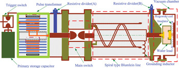
Figure 1 shows the schematic of the IEBA, which was capable of generating a quasi-square wave with voltage of 100–600kV by adjusting the gas pressure of the main switch, and full width at half maximum (FWHM) of 180 ns when connected to impedance-matched load of 10 Ω. The IEBA consisted of a 50 kV, 12 µF primary storage capacitor, a 50 kV field distortion trigger switch, a spiral strip type pulsed transformer (Liu et al., Reference Liu, Zhan, Zhang, Liu, Feng, Shu, Zhang and Wang2007) with output voltage up to 600 kV, main switch with sulfur-hexafluoride (SF6) used as insulating medium, strip spiral type BPFL with impedance of about 10 Ω, vacuum chamber which was pumped by the combination of mechanical and molecular pumps to keep the vacuum degree up to 10−3 Pa, voltage and current diagnostic system. To generate the electron beam, a field-emission diode is usually used. However, to test the operating characteristics of IEBA, a high power water load is usually used (Han et al., Reference Han, Kim, Park, Yoon and Park2009), and the “water” is a solution of CuSO4 of a concentration that is adjusted to match the impedance of the BPFL.
(Color online) Schematic of the intense electron beam accelerator based on strip spiral type Blumlein line.

Just as shown in Figure 1, a resistive divider (A), which is placed between the output terminal of the pulse transformer and main switch, was used to measure the charging voltage of the BPFL, and resistive divider (B) was also placed on the output terminal of the BPFL to measure the load voltage. A Rogowski coil was used to measure the load current.
The operating process of the IEBA was as follow. When the charging voltage of the primary storage capacitor reached a certain value, the field distortion trigger switch was triggered and closed, and then the primary storage capacitor discharged to the primary winding of the transformer consequently, the transformer started to charge the BPFL. Once the charging voltage of the BPFL reached the breakdown value of the main switch, the BPFL discharged to the load, and a quasi-square wave with a rise time approximately 30 ns and FWHM of 180 ns was formed. The amplitude of the quasi-square wave could be adjusted from 100 kV to 600 kV by changing the gas pressure (Pm = 0–0.50 MPa) of the main switch, so the output peak power could be up to 30 gigawatt.
Obviously, to investigate the operating characteristics of IEBA, the impedance of the water load should be adjusted. In this paper, four typically load conditions are discussed, load matching, load short, load open, and surface flashover in the vacuum chamber. Load matching, it means that the impedance of the load is equal to that of the BPFL, and IEBA is usually operated at this kind of conditions. Load short, the impedance of the load is less than 1 Ω. Load open; there is no load in the IEBA. In other words, the impedance of the load is infinite. As we know, the vacuum chamber in Figure 1 is used to assemble the load, and the surface flashover may occur along the insulator, also, if water load is used, the surface flashover may also occur along the water load (Cheng et al., Reference Cheng, Liu, Zhang, Hong and Qian2011), so this kind of condition will also be discussed. Load sort, load open and surface flashover in the vacuum chamber, which mean that the IEBA operates at abnormal conditions, and the effect of these abnormal conditions on the operating characteristics of IEBA.
3. DISCUSSION ON THE OPERATING CHARACTERISTICS
3.1. Load Matching
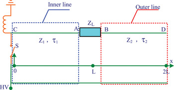
The Blumlein PFL consists of three coaxial cylindrical lines filled with de-ionized water as dielectric. The PFL formed by the inner conductor and the middle conductor are usually called the inner line. If the PFL is formed by the middle conductor and the outer conductor, it is called the outer line. The wave impedances of the inner line and outer line are Z 1 and Z 2, respectively. So during the Blumlein line discharge into the load, the equivalent circuit of the Blumlein line is shown in Figure 2. Where S is the main switch, CA is the inner line, BD is the outer line, and ZL is the load. Also, the voltage measured by the resistive divider (A) in Figure 1 is just the output voltage of the HVPT. The voltage at point D in Figure 2 is also just the voltage at the output terminal of HVPT. In order to get the voltage at the output terminal of HVPT, the voltage at point D need to be solved, so a coordinate system is built in Figure 2; the main switch is the zero point. When PFL is charged to a voltage U(U < 0), once the main switch S is closed, the PFL can not stay in equilibrium since the PFL elementary capacitors adjacent to the load Z L start discharging. So the voltages at the inner line and outer line satisfied the equations
(Color online) Equivalent circuit of the BPFL discharge into the load.

 $$\left\{\matrix{ - \displaystyle{{\partial u_1 \lpar x\comma \; t\rpar \over \partial x}} = L_i \displaystyle{{\partial i_1 \lpar x\comma \; t\rpar \over \partial t}} \cr - \displaystyle{{\partial i_1 \lpar x\comma \; t\rpar \over \partial x}} = C_i \displaystyle{{\partial u_1 \lpar x\comma \; t\rpar \over \partial t}} } \right. \;\left\{\matrix{ - \displaystyle{{\partial u_2 \lpar x\comma \; t\rpar \over \partial x}} = L_o \displaystyle{{\partial i_2 \lpar x\comma \; t\rpar \over \partial t}} \cr - \displaystyle{{\partial i_2 \lpar x\comma \; t\rpar \over \partial x}} = C_o \displaystyle{{\partial u_2 \lpar x\comma \; t\rpar \over \partial t}} } \right. \cdot$$
In the above equations, L i, C i, u 1(x, t), i 1(x, t) and L o, C o, u 2(x, t), i 2(x, t)are inductances of per unit, capacitances of per unit, voltages, and currents of the inner line and outer line, respectively. And the transmission time and impedance of inner and outer line is
 $$\left\{\matrix{{\rm \tau} _1 = L\sqrt {L_i C_i } \cr Z_1 = \sqrt {L_i /C_i } } \right. \;\left\{\matrix{{\rm \tau} _2 = L\sqrt {L_o C_o } \cr Z_2 = \sqrt {L_o /C_o } } \right.\; \cdot$$
One should note that if the middle conductor is replaced by a spiral strip middle cylinder, τ 1 is usually not equal to τ 2. Here, τ 1 is usually equal to τ 2, and it is assumed that
 $${\rm \tau} _1 = {\rm \tau} _2 \equiv {\rm \tau} \cdot$$
When t = 0, the initial conditions of Eq. (1) are
 $$\left\{\matrix{u_1 \lpar x\comma \; 0\rpar = u_2 \;\lpar x\comma \; 0\rpar = U \cr i_1 \lpar x\comma \; 0\rpar = i_2 \;\lpar x\comma \; 0\rpar = 0 } \right. \cdot$$
And for the characteristic of the PFL, the boundary conditions are
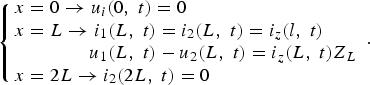 $$\left\{\matrix{x = 0 \to u_i \lpar 0\comma \; t\rpar = 0 \cr x = L \to i_1 \lpar L\comma \; t\rpar = i_2 \lpar L\comma \; t\rpar = i_z \lpar l\comma \; t\rpar \cr \quad \quad \quad \quad u_1 \lpar L\comma \; t\rpar - u_2 \lpar L\comma \; t\rpar = i_z \lpar L\comma \; t\rpar Z_L \cr x = 2L \to i_2 \lpar 2L\comma \; t\rpar = 0 } \right. \cdot$$
So, the load voltage could be solved by Eqs. (1)–(5)
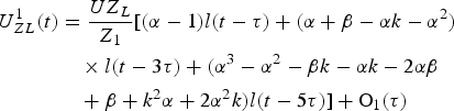 $$\eqalign{U_{ZL}^1 \lpar t\rpar &= \displaystyle{{UZ_L } \over {Z_1 }}\lsqb \lpar {\rm \alpha} - 1\rpar l\lpar t - {\rm \tau} \rpar + \lpar {\rm \alpha} + {\rm \beta} - {\rm \alpha} k - {\rm \alpha} ^2 \rpar \cr &\quad \times l\lpar t - 3{\rm \tau} \rpar + \lpar {\rm \alpha} ^3 - {\rm \alpha} ^2 - {\rm \beta} k - {\rm \alpha} k - 2{\rm \alpha} {\rm \beta} \cr &\quad + {\rm \beta} + k^2 {\rm \alpha} + 2{\rm \alpha} ^2 k\rpar l\lpar t - 5{\rm \tau} \rpar \rsqb + {\rm O}_1 \lpar {\rm \tau} \rpar}$$
Where  ${\rm \alpha} = \displaystyle{{Z_2 + Z_L - Z_1 } \over {Z_2 + Z_1 + Z_L }}\comma \; {\rm \beta} =\displaystyle{{Z_2 + Z_1 - Z_L } \over {Z_2 + Z_1 + Z_L }}\comma \; - k =$
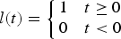
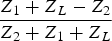 $ \displaystyle{{Z_1 + Z_L - Z_2 } \over {Z_2 + Z_1 + Z_L }}$, and O1 (τ) stands for the remainder, when t < 7τ, O1 (τ) ≡ 0. l(t) is the step function, and it is defined as
 $$l\lpar t\rpar = \left\{\matrix{1 &t \geq 0 \cr 0 &t \lt 0 } \right.$$
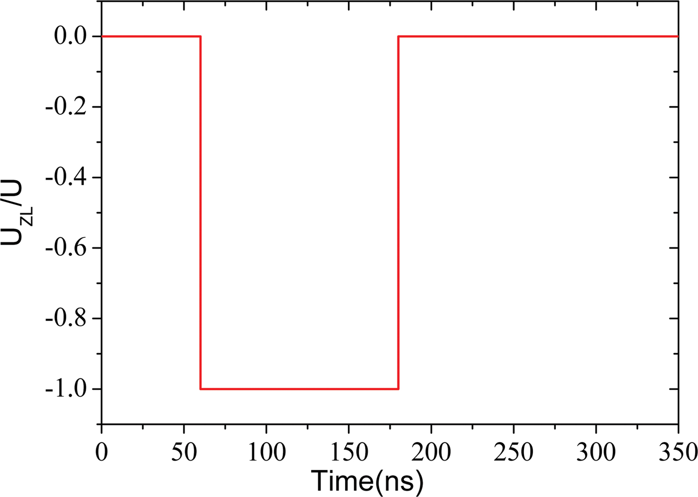
When the BPFL is designed as Z 1 = Z 2 and the load is matched with the BPFL (Z L = Z L + Z 2), the waveform of load voltage could be obtained by Eq. (6), which is shown in Figure 3.
(Color online) Load voltage when the impedance of load is matched with BPFL (τ = 60 ns).
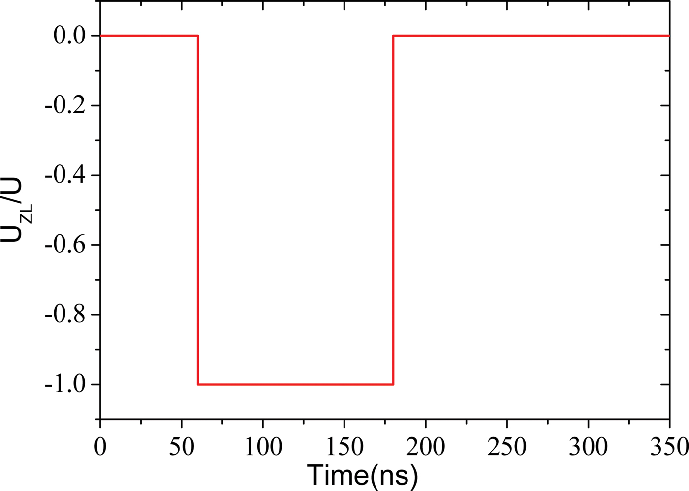
In Figure 3, it is obtained that when the impedance of load is matched with BPFL, the output voltage waveform of IEBA is a square wave, and the amplitude of output voltage is equal to that of charging voltage. Meanwhile, at this kind of condition, once the main switch is closed, according to Eqs. (1)–(5), the voltage at the output terminal of HVPT is
 $$U_C^1 \lpar t\rpar = U\lsqb 1 - l\lpar t - 2{\rm \tau} \rpar \rsqb.$$
Obviously, when the load is matched with the BPFL, once the main switch is closed, the the voltage at the output terminal of HVPT turns to zero.
3.2. Load Short
When the load is short, the impedance of load is very small, even zero. Obviously, the load voltage is zero. However, the voltage at the output terminal of HVPT should be recalculated. First, we discuss Z 1 = Z 2 and τ1 = τ1 = τ2 ≡ τ. if Z L ≠ Z 1 + Z 2, as the same method, from Eqs. (1)–(4) leads to (Cheng et al., Reference Cheng, Liu, Qian, Zhang and Zhang2009b)
 $$U_C^2 \lpar t\rpar = U\lcub 1 - {\rm \gamma} \sum\limits_{n = 0}^\infty {{\rm \zeta} ^n } l\lsqb t - \lpar 4n + 2\rpar {\rm \tau} \rsqb \rcub.$$
Where  ${\rm \zeta} = \displaystyle{{Z_L - Z_1 - Z_2 } \over {Z_2 + Z_1 + Z_L }}, {\rm \gamma} = \displaystyle{{4Z_2 } \over {Z_1 + Z_2 + Z_L }}$. So the voltage at the output terminal of HVPT is a damped bipolar oscillation wave, and the peak voltage is determined by ζ and γ. When Z L→0, γ→2, ζ→ − 1, the amplitude of oscillation is much bigger and the damping of the bipolar oscillating voltage is smaller. If Z L = 0, this provide a short circuit for the Blumlein line, so ζ = −1, γ = 2, ζ = − 1, γ = 2, the voltage at the output terminal of HVPT is
 $$U_C^3 \lpar t\rpar = U\lcub 1 - 2\sum\limits_{n = 0}^\infty {\lpar - 1\rpar ^n } l\lsqb t - \lpar 4n + 2\rpar {\rm \tau} \rsqb \rcub.$$
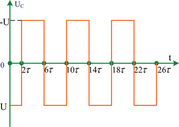
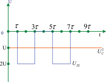
Figure 4 is the waveform of the voltage at the output terminal of HVPT when the load is short. It clearly shows that the voltage at the output terminal of HVPT is a bipolar rectangular wave with a period of 8τ and duty ratio of 50%. It is obtained that the oscillation frequency is determined by the duration of the BPFL.
(Color online) The voltage at the output terminal of HVPT when Z 1 = Z 2, Z L = 0.

So at Z L → 0, there will be a bipolar oscillating voltage at the output terminal of HVPT, which is disadvantageous for the operation of the HVPT, because surface flashover occurred unexpectedly at low fields under the bipolar oscillating voltage, Miller et al. (Reference Miller, Prestwich, Poukey, Epstein, Freeman, Sharpe, Tucker and Shope1981) and Adler et al. (Reference Adler, Miller, Prestwich and Smith1983) found this phenomenon. Also the critical flashover voltage decreases with the increment of the angle frequency of the oscillating voltage, and for the same critical flashover voltage, the flashover distance increases with the increment of the applied voltage (Pai & Zhang, Reference Pai and Zhang1995). When the impedance of load becomes small or zero, this makes it easier for surface flashover along the insulation materials to form and decrease the lifetime of the HVPT. Hence, in order to avoid the surface flashover, the insulation materials of the HVPT need to be improved and the impedance of load should not be too small.
Also, if Z 1 ≠ Z 2, Z L ≠ Z 1 + Z 2. The voltage at the output terminal of HVPT could be obtained from Eqs. (1)–(4)
 $$U_C^{\rm 4} \lpar t\rpar = U\lcub 1 - {\rm \gamma} \sum\limits_{n = 0}^{\infty} \sum\limits_{\,j = 0}^m \displaystyle{{\lpar n - j\rpar ! \over \,j!\lpar n - 2j\rpar !}} {\rm \xi}^{n - 2j} {\rm \zeta}^j\, {\bf \cdot} l\lsqb t - \lpar 2n + 2\rpar {\rm \tau} \rsqb \rcub.$$
In Eq. (11), m = n/2 for n being an even number and m = (n − 1)/2 for n being an odd number. 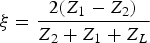 ${\rm \xi} = \displaystyle{{2\lpar Z_1 - Z_2 \rpar } \over {Z_2 + Z_1 + Z_L }}$. Obviously, when Z L → 0, the voltage at the output terminal of HVPT is still a damped bipolar oscillation wave, but there may be γ > 2, so the amplitude of oscillation is much bigger and the damping of the bipolar oscillating voltage is smaller.
3.3. Load Open
When the load is open, the impedance of load is infinite. In other words, the impedance of load is much larger than the impedance of BPFL. We just discussed the ideal equivalent circuit of the BPFL discharge into the load (see Fig. 3). Once the main switch is closed, the load voltage and the voltage at the output terminal of HVPT could be obtained from Eq. (6) and Eq. (8), respectively, when τ1 = τ2 ≡ τ, Z 1 = Z 2Z L ≫ Z 1 + Z 2.
The ideal load voltage and the voltage at the output terminal of HVPT are shown in Figure 5, it is obtained that the voltage at the output terminal of HVPT is a constant valve, and which is just the charging voltage. Meanwhile, the load voltage is a periodic rectangular wave with a period of 4τ and duty ratio of 50%, and the amplitude of the load voltage is twice the charging voltage.
(Color online) Ideal load voltage and voltage at the output terminal of HVPT when τ1 = τ2 ≡ τ, Z 1 = Z 2Z L ≫ Z 1 + Z 2.

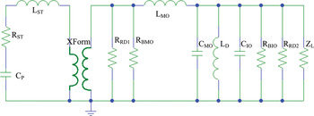
However, when the load is open, grounding inductor and resistor of the resistive divider (B) in Figure 1 has a great effect on the load voltage and the voltage at the output terminal of HVPT. Once the main switch (ideal switch) is closed, the actual discharging circuit of IEBA is shown in Figure 6.
(Color online) After the main switch is closed, the discharging circuit of IEBA when the load is open.

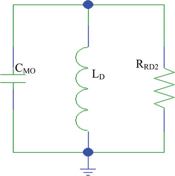
As shown in Figure 6, CP is the primary energy-storage capacitance, and RST and LST are the resistance and inductance of primary winding circuit, HVPT are modeled by XForm2 in the circuit, RRD1 (tens of kilohm) is the resistance of resistive divider (A) in Figure 1, RBMO (megohm level) is the bleeder resistance of outer line, LMO (less than microhenry) and CMO is the inductance and capacitance of outer line, respectively, LD is the grounding inductor, CIO and RBIO is capacitance and bleeder resistance of the output pulse forming line, respectively, and CIO is much less than CMO, RRD2 (about 2 kilohm) is the resistance of resistive divider (B) in Figure 1, ZL is the load of IEBA, when the load is open, ZL is about megohm level. So according to the circuit and value of the parameters, the discharging circuit could be simplified as Figure 7.
(Color online) Simplified discharging circuit of IEBA when the load is open.

In Figure 7, C MO = τ2/Z 2 and considering that 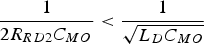 $\displaystyle{1 \over {2R_{RD2} C_{MO} }} \lt \displaystyle{1 \over {\sqrt {L_D C_{MO} } }}$, the voltage at the output terminal of HVPT is
 $$U_C^4 \lpar t\rpar = \displaystyle{U \over {\rm \omega} } \times e^{ - {\rm \delta} t} \lsqb {\rm \omega} Cos\lpar {\rm \omega} t\rpar - {\rm \delta} Sin\lpar {\rm \omega} t\rpar \rsqb.$$
Where  ${\rm \omega} = \sqrt {{\rm \omega} _0^2 - {\rm \delta} ^2 } \comma \; {\rm \omega} _0 = \displaystyle{1 \over {\sqrt {L_D C_{MO} } }}\comma \; {\rm \delta} = \displaystyle{1 \over {2R_{RD2} C_{MO} }}$. In Eq. (12), it is obvious that the voltage at the output terminal of HVPT is not a constant value when the load is open. The voltage at the output terminal of HVPT is a damped bipolar oscillation wave, and the oscillation frequency is decided by the parameter of outer line, grounding inductor, and resistance of resistive divider (B). Then, submitting these parameters into Eq. (12), the voltage at the output terminal of HVPT and its oscillation frequency could be obtained. Of course, the load voltage will be changed with the voltage at the output terminal of HVPT, and the load voltage is
 $$U_{ZL}^2 \lpar t\rpar = R_{RD2} \times i_{R_{RD2} } \lpar t\rpar = L_D \displaystyle{{di_{L_D } \lpar t\rpar } \over {dt}}.$$
Where  $i_{R_{RD2} } \lpar t\rpar$ is the current of resistive divider (B),
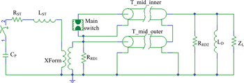
 $i_{L_D } \lpar t\rpar$ is the current of grounding inductor. Then to clearly shown the effect of the grounding inductor on the voltage at the output terminal of HVPT and load voltage, PSPICE circuit analysis was used to simulate the accelerator based on HVPT and BPFL when the load is open. Figure 8 shows schematically the full circuit model. The whole circuit is connected to components built in PSPICE component storage or modeled by the authors according to the performance of the device.
(Color online) PSPICE circuit schematic used to model the IEBA.

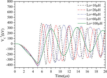
In Figure 8, T_mid_inner and T_mid_outer are connected in parallel to simulate the BPFL. And in the simulation, supposing τ1 = τ 2 ≡ 60 ns, Z 1 = Z 2 = 6 Ω and Z L = 100 MΩ, The output voltage of the HVPT can be obtained at different grounding inductor. Figure 9 shows the simulation results.
(Color online) The voltage at the output terminal of HVPT for different grounding inductor when the load is open.

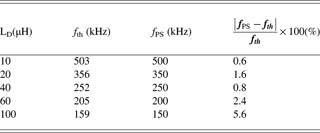
It is shown that the main switch is closed at time of 5 µs, and then the voltage at the output terminal of HVPT is a damped bipolar oscillation wave. At different grounding inductor, the oscillation wave is difference. Also, according to Figure 9, the oscillation frequency of the voltage at the output terminal of HVPT could be obtained by Fourier analysis. Meanwhile, submitting the parameters that are used in the PSPICE simulation to Eq. (12), the oscillation frequency also could be calculated theoretically.
In Table 1, as the increment of the inductance of the grounding inductor, the oscillation frequency is decreased. Also, the theoretical results are almost the same as that of PSPICE simulation. So, the grounding inductor has a great effect on the load voltage and the voltage at the output terminal of HVPT when the load is open. Obviously, once the main switch is closed, the load voltage is twice the charging voltage of BPFL. However, as the oscillation of the voltage at the output terminal of HVPT, the load voltage would be an oscillation waveform.
Theoretical calculated and PSPICE simulated oscillation frequency of the voltage at the output terminal of HVPT
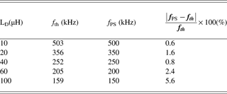
Figure 10 shows the typical load voltage at load open, it clearly shows that once the main switch is closed, the amplitude of the load voltage is twice the charging voltage of BPFL, which is similar with that in Figure 5. Subsequently, the voltage at the output terminal of HVPT is decreased, which causes the amplitude of the load voltage to be reduced. The amplitude of the load voltage is changed with the oscillation of the voltage at the output terminal of HVPT.
(Color online) PSPICE simulated load voltage and voltage at the output terminal of HVPT for load open when L D is 60 µH.

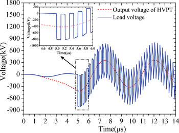
To further verify the correctness of the theoretically results, an experiment was performed on an IEBA based on spiral type Blumlein line, the transmission time and impedance of inner line are 70 ns and 6.4 Ω, the outer line are 76 ns and 4 Ω. The experimental waveform of load voltage and the voltage at the output terminal of HVPT are shown in Figure 11.
(Color online) Experimental load voltage and voltage at the output terminal of HVPT for load open when L D is 60 µH.

In Figure 11, the voltage at the output terminal of HVPT is still an oscillation wave, which is similar with that in Figure 10. Also, the amplitude of the first main pulse of load voltage is about twice that of the voltage at the output terminal of HVPT. Meanwhile, the amplitude of the load voltage is also changed with the oscillation of the voltage at the output terminal of HVPT. However, there is a little difference on the characteristics of load voltage. Comparing with the waveform in Figure 10, the amplitude of load voltage in Figure 11 is damped quickly. In fact, the main switch is not an ideal switch, so during the experiments, the resistance of the switch channel can not be ignored, and energy may be dissipated in the main switch. Then, adding the resistance of the switch channel into Figure 8, the waveform of load voltage can be recalculated in Figure 12.
(Color online) PSPICE simulated load voltage at difference resistance of main switch when load open.

In Figure 12, it is obtained that the load voltage at difference resistance of switch channel is difference. For ideal condition, R S = 0.001 Ω the amplitude of the load voltage is damped very slowly, which is similar with that in Figure 10. However, when the resistance of switch channel is up to 0.1 Ω, even to 0.5 Ω, the amplitude of the load voltage is damped quickly, and the waveform is similar with that in Figure 11.
One should note that the voltage at the output terminal of HVPT is oscillation waver when the load is short and open, but the oscillation frequency is difference. For example, the period of the oscillation wave is about 8τ (480 ns) and 5 µs when the load is short and open, respectively. Of course, the effect on the HVPT is also difference, and the output voltage has a greater effect on the HVPT when the load is short.
3.4. Surface Flashover in the Vacuum Chamber
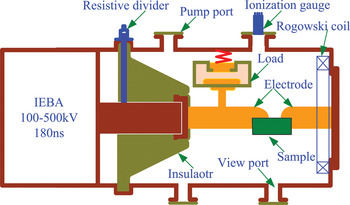
Vacuum chamber is one of the important parts of IEBA, and it is used to place the load. However, if surface flashover occurs along the insulator that is used to support the inner cylinder of the BPFL, the operating characteristics of IEBA could be changed. So, the operating characteristics of the IEBA should be investigated when the surface flashover occurs in the vacuum chamber. In most conditions, the surface flashover does not occur, because of that the insulator is designed to avoid surface flashover occur. So to research the operating characteristics of IEBA when the surface flashover occurs, a sample should be used to simulate the surface flashover that occurs along the insulator, as shown in Figure 13.
(Color online) Schematic of the vacuum chamber.

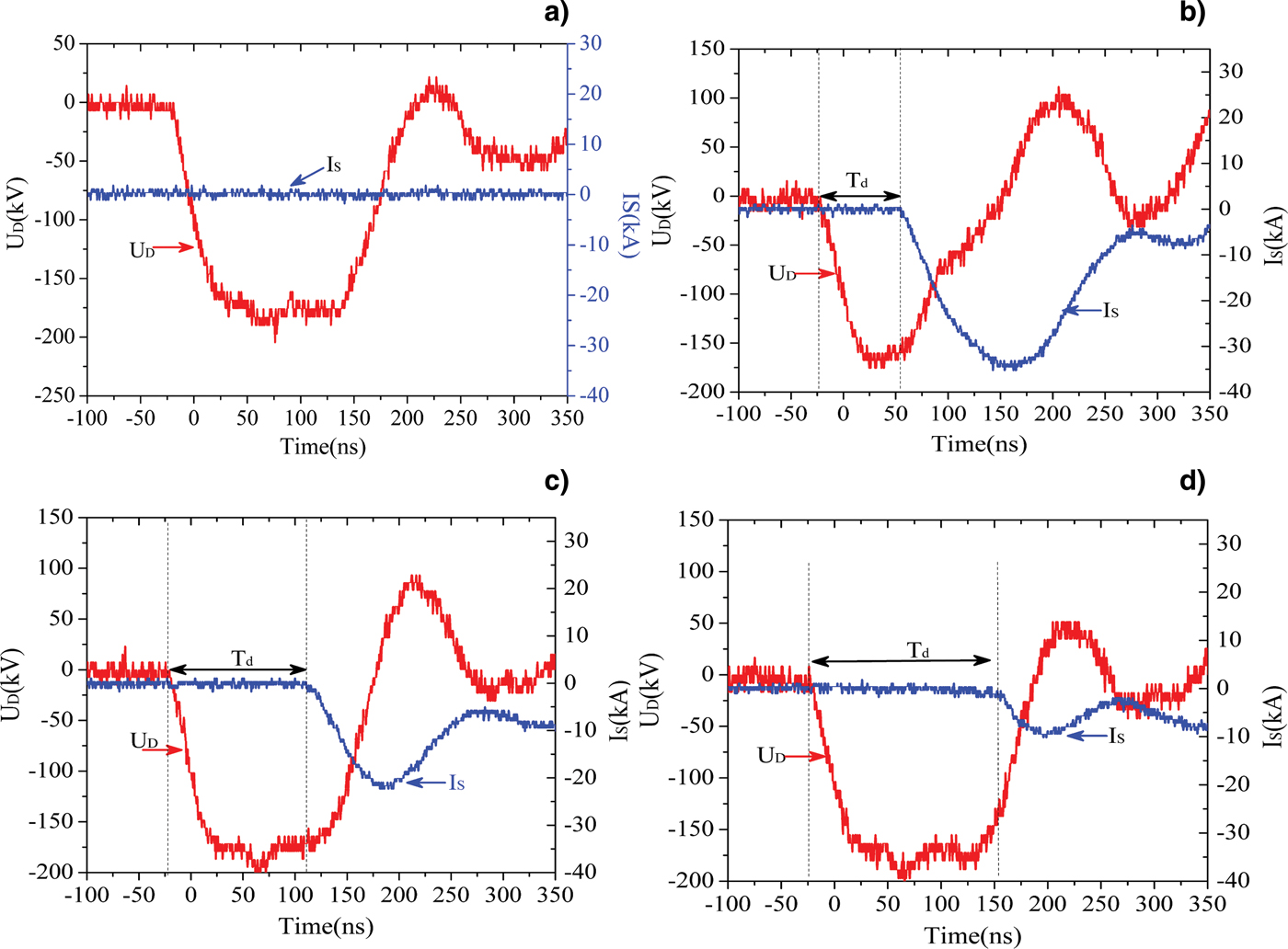
In Figure 13, the material of the sample is high density polyethylene (HDPE), and the sample is place between electrodes. The gap spacing could be adjusted by changing the electrode and dimension of the sample. So the surface flashover could be controlled by the load voltage and gap spacing. Figure 14 shows the typical waveform of load voltage and surface flashover current at different gap spacing.
(Color online) Typical waveform of flashover at voltage of 180 kV, (a) No sample, (b) D = 100 mm, (c) D = 170 mm, (d) D = 210 mm.
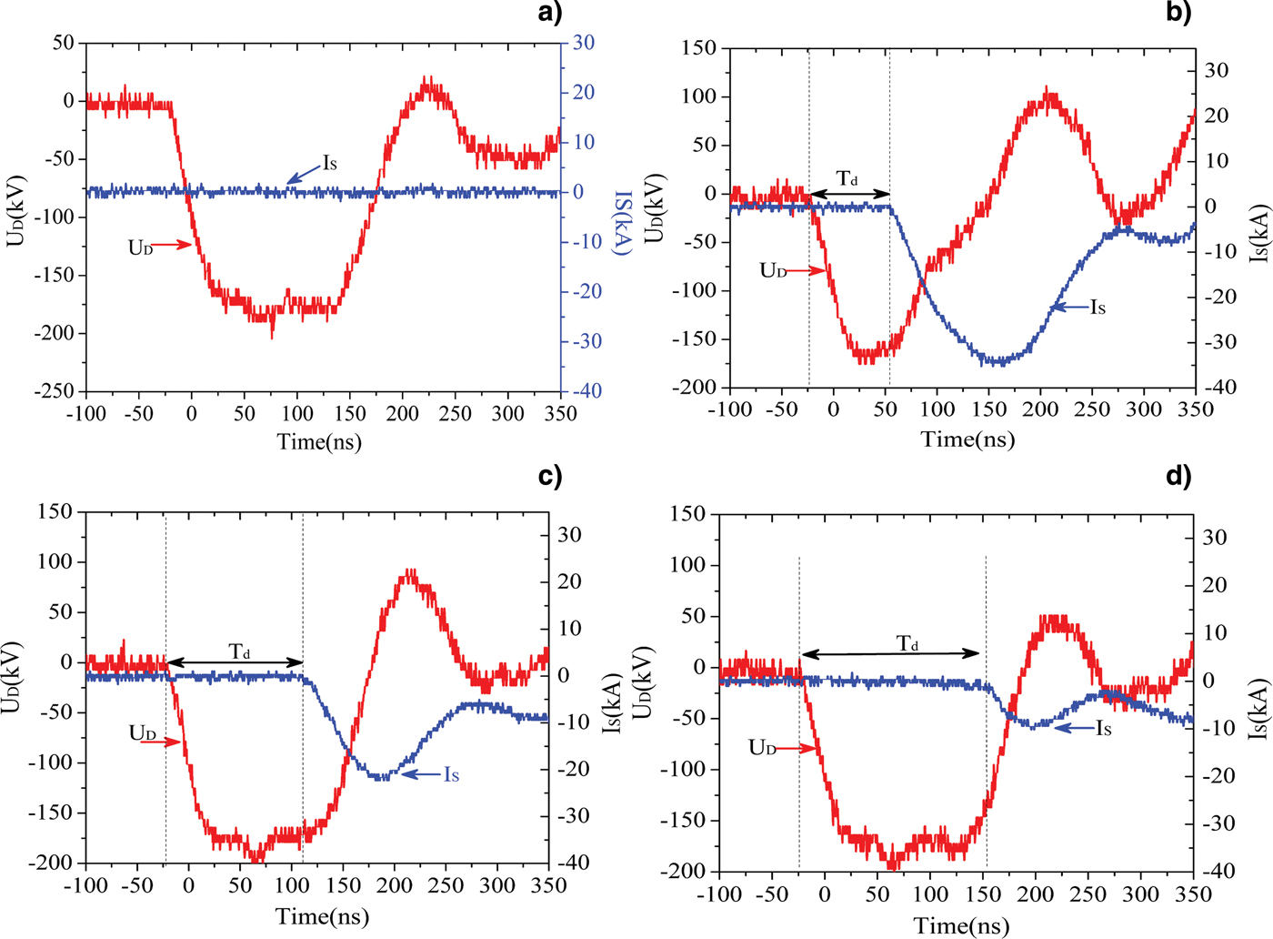
In Figure 14a, it was shown that, before adding the sample, the load voltage was a typical quasi-square wave with voltage of 180 kV and FWHM of 180 ns, and the surface flashover current measured by a Rogowski coil in Figure 13 is zero. After adding the sample, surface flashover occurs, but the time at which the surface flashover occurs is not the same. If the pre-breakdown delay time is defined as the time from the load voltage rise to the load voltage drop due to surface breakdown (or flashover current starts) (see Fig. 14), it is obtained that the delay time is increased with the increment of the gap spacing. Also, one should be noted that the FWHM of the load voltage is changed, before adding the sample, the FWHM is about 180 ns. However, after adding the sample with gap spacing of 100 mm, the FWHM is only 98 ns (Fig. 14b) and the flashover current is very high, which is up to 34 kA. When the gap spacing is increased to 170 mm, the FWHM is also increased to 160 ns (Fig. 14c), and the flashover current is decreased to 21 kA. In other words, the surface flashover in the vacuum chamber will affect the FWHM of the output voltage. But if the surface flashover occurs after the main pulse of the output voltage, there is little effect on the FWHM of the output voltage, such as Figure 14d, the FWHM is also up to 170 ns, and the flashover current is further decreased to 10 kA.
According to the above, one conclusion could be obtained, if the flashover occurred at the flat part of the main pulse, the value of the peak flashover current was very high, and which will decrease the FWHM of the output voltage. However, if the flashover occurred after the main pulse, there was little effect on the output voltage of IEBA. So, during the operation of the IEBA, it must be avoided that the flashover occurred at the flat part of the main pulse.
When the surface flashover occurs, the impedance of the load is less than 1 Ω. So the characteristic of the voltage at the output terminal of HVPT is similar with that of load short. Once the surface flashover occurs in the vacuum chamber, the voltage at the output terminal of HVPT would be a damped bipolar oscillation wave. In Cheng et al. (Reference Cheng, Liu, Zhang, Hong and Qian2011), we have reported the results. In a word, the output voltage of IEBA and the voltage at the output terminal of HVPT are all affected by the surface flashover in the vacuum chamber, so which should be avoided during the operation of IEBA.
4. CONCLUSIONS
Through the analysis of theoretical calculation, PSPICE simulation, and experiment studying, the operating characteristics of IEBA based on HVPT and BPFL are discussed at different load conditions, load matching, load short, load open, and surface flashover in the vacuum chamber. Some conclusions can be made as follows: (1) when the load is matched with BPFL, the load voltage is a well squared wave and the voltage at the output terminal of HVPT is turned zero. (2) There will be an oscillation wave at the output terminal of HVPT when the load is short, which affects the electrical insulation of HVPT and decreases its lifetime. (3) When the load is open, once the main switch is closed, the amplitude of the main pulse of load voltage is twice the charging voltage of BPFL. Meanwhile, the voltage at the output terminal of HVPT is also an oscillation wave, which causes that the amplitude of the load voltage is reduced. (4) When surface flashover occurs in the vacuum chamber, the FWHM of the load voltage is decreased. Also, the voltage at the output terminal of HVPT would be a damped bipolar oscillation wave. So, to make the IEBA operate well, load short, load open and surface flashover in the vacuum should be avoided during the operation of IEBA.
ACKNOWLEDGMENTS
The authors gratefully acknowledge the support from the Fund of innovation, Graduate school of National University of Defense Technology (NUDT) under Grand No. B090701 and National Natural Science Foundation of China (51177167)