1 Introduction
Viscous fingering occurs when a less viscous fluid displaces a more viscous fluid in a porous medium (Saffman & Taylor Reference Saffman and Taylor1958; Homsy Reference Homsy1987). A perturbation at the interface between the two fluids grows because a favourable pressure gradient is generated at the location(s) where the less viscous fluid locally extends into the more viscous fluid. One classic categorisation of viscous fingering is based on whether the two fluids are miscible or immiscible. In the immiscible case, surface tension at the interface provides a restoring force that tends to smooth the instability, while in the miscible case, the absence of any restoring force results in all wavenumbers being unstable. An example of the striking contrast in patterns is provided by Chen (Reference Chen1987), who shows fine fingers for water displacing glycerol, but rounded, lobe-like fingers for oil displacing glycerol.
While both miscible and immiscible fingering have been extensively studied in the classic configuration, the idea of viscous fingering has been combined with other physics to enrich the parameter space and the observed features. Examples range from the use of non-Newtonian fluids (Lindner et al. Reference Lindner, Bonn, Poiré, Amar and Meunier2002) to spatially varying permeabilities (Pihler-Puzović et al. Reference Pihler-Puzović, Périllat, Russell, Juel and Heil2013) to chemical reactions (De Wit & Homsy Reference De Wit and Homsy1999). One such extension is the effect of suspended particles in one or both of the fluids. Tang et al. (Reference Tang, Grivas, Homentcovschi, Geer and Singler2000) experimentally revealed that a uniform suspension of particles injected radially into a Hele-Shaw cell could exhibit viscous fingering due to the accumulation of particles near the suspension–air interface, which arises from shear-induced migration (Leighton & Acrivos Reference Leighton and Acrivos1987). This local accumulation of particles near the interface results in a flow in which a low-concentration, low-viscosity suspension displaces a high-concentration, high-viscosity suspension, and this flow is inherently unstable due to the classic mechanism.
More recently, Xu, Kim & Lee (Reference Xu, Kim and Lee2016) and Kim, Xu & Lee (Reference Kim, Xu and Lee2017) experimentally investigated the radial flow of a suspension of non-colloidal particles in a Hele-Shaw cell initially filled with air. Similar to Tang et al. (Reference Tang, Grivas, Homentcovschi, Geer and Singler2000), a band of high-concentration suspension spontaneously formed near the suspension–air interface, which was displaced by a lower-concentration suspension injected from the centre. In this way, there were three fluids: low-concentration suspension, high-concentration suspension and air. As flow continued, the inner miscible interface deformed, and a pattern of rounded, lobe-like fingers penetrated into the band of high-concentration suspension. The observed pattern lacked high-wavenumber disturbances and was reminiscent of immiscible viscous fingering. This raises the question of what stabilises the interface between the low- and high-concentration suspensions with zero surface tension and suppresses the fine fingers characteristic of miscible fingering.
In this work, we address this question by hypothesising that the interplay between the unstable miscible and stable immiscible interfaces may lead to fingers with a finite wavenumber at the miscible interface. We first present experimental details of the observations of this instability. We then conduct a linear stability analysis for multiple layers of fluid; the analysis is similar to that by Cardoso & Woods (Reference Cardoso and Woods1995) with the distinction that, in the present case, the interface between low-concentration suspension and high-concentration suspension is miscible, and there is a particle flux across it. Additionally, we incorporate the effect of normal viscosity (Kim et al. Reference Kim, Funada, Joseph and Homsy2009) in the present analysis. The resultant critical wavenumber shows that surface tension on the suspension–air interface can damp high-wavenumber disturbances on the miscible interface in good agreement with experiments.
2 Experiments
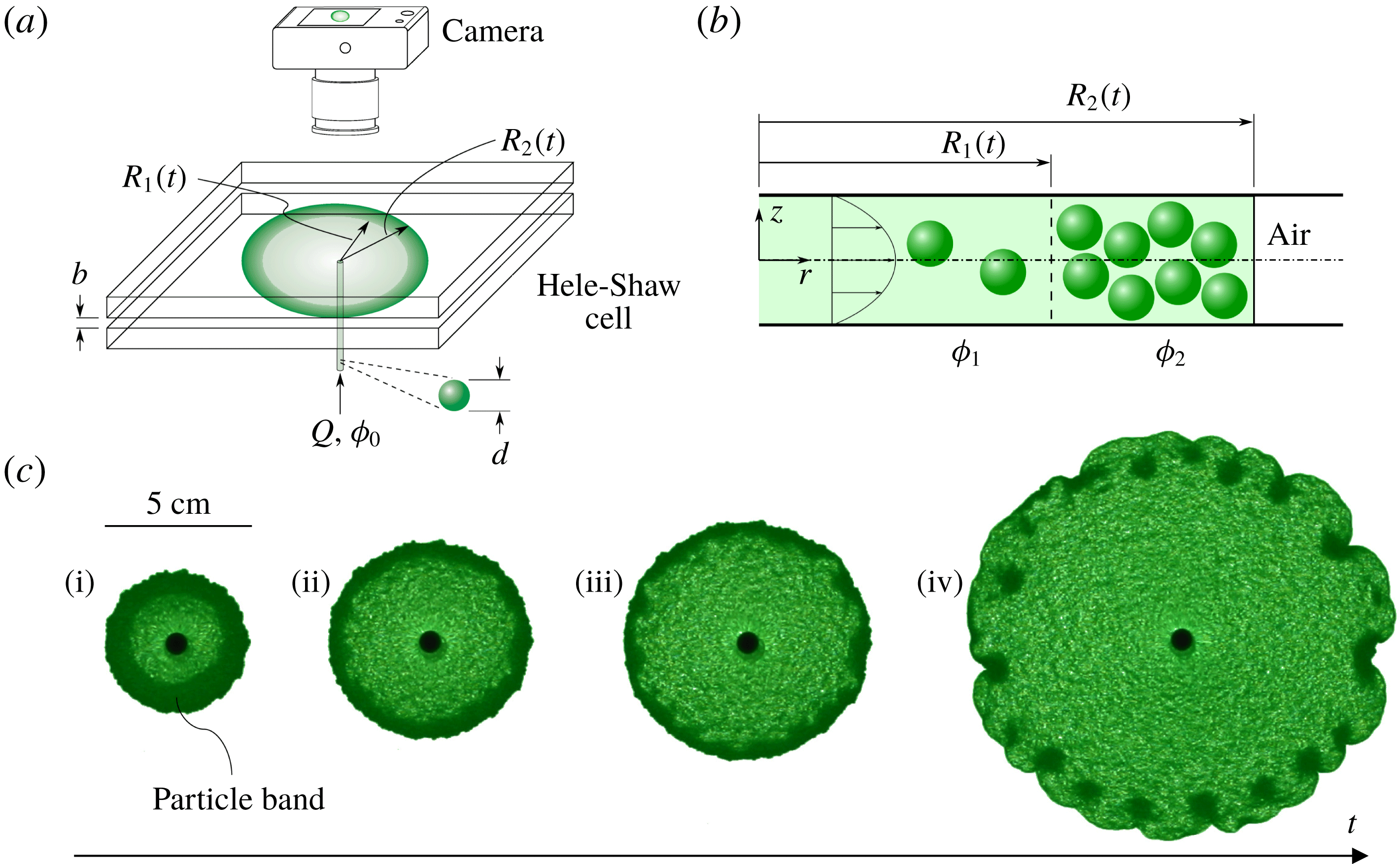
A suspension of non-colloidal polyethylene particles in silicone oil is injected into a Hele-Shaw cell and flows radially outwards, displacing quiescent air (see figure 1(a)). The particles (Cospheric) have a nominal diameter
 $d=325\,\unicode[STIX]{x03BC}\text{m}$
(
 $300\,\unicode[STIX]{x03BC}\text{m}\leqslant d_{particles}\leqslant 355\,\unicode[STIX]{x03BC}\text{m}$
), density
 $\unicode[STIX]{x1D70C}_{p}=1.0\,\text{g}~\text{cm}^{-3}$
and are dispersed in silicone oil (UCT), which has a density
 $\unicode[STIX]{x1D70C}_{l}=0.96\,\text{g}~\text{cm}^{-3}$
, dynamic viscosity
 $\unicode[STIX]{x1D707}_{l}=0.096\,\text{Pa}~\text{s}$
and interfacial tension with air of
 $\unicode[STIX]{x1D6FE}_{\text{o/a}}=18.7\,\text{mN}~\text{m}^{-1}$
(Ricci, Sangiorgi & Passerone Reference Ricci, Sangiorgi and Passerone1986). The suspension is mixed to the specified solid volume fraction
 $\unicode[STIX]{x1D719}_{0}$
in a syringe and injected with a syringe pump (New Era) through a plastic tube (inner diameter
 $4.7\,\text{mm}$
, length
 $L=1\,\text{m}$
) into the Hele-Shaw cell at a constant flow rate
 $Q=75$
,
 $100$
or
 $150\,\text{mL}~\text{min}^{-1}$
. The Hele-Shaw cell consists of two glass plates separated by a gap of thickness
 $b$
with a hole of diameter
 $d_{hole}=7.9\,\text{mm}$
in the centre of the bottom plate. The experiments are backlit by an LED panel (ASD Lighting) and imaged from above by a digital camera (Nikon D500). Two parametric studies are conducted to probe the effects of
 $b$
and
 $\unicode[STIX]{x1D719}_{0}$
on the observed instability. In the first, the particle concentration is held fixed at
 $\unicode[STIX]{x1D719}_{0}=0.30$
, while
 $b$
ranges from
 $635\,\unicode[STIX]{x03BC}\text{m}$
to
 $1400\,\unicode[STIX]{x03BC}\text{m}$
. In the second,
 $b=1020\,\unicode[STIX]{x03BC}\text{m}$
, and
 $\unicode[STIX]{x1D719}_{0}$
is varied over the range
 $0.15\leqslant \unicode[STIX]{x1D719}_{0}\leqslant 0.35$
.
(a) Schematic of the experimental set-up. (b) Cross-sectional schematic of particles jamming at the suspension–air interface. (c) Characteristic images of instability growth in a band of high-concentration suspension: (i–ii) High-concentration outer band with lower-concentration suspension in the middle expanding and thinning over time (
 $t=0.2{-}0.9~\text{s}$
). (iii) Onset of instability in the particle band showing disturbance of the interface between low- and high-concentration regions at
 $t=1.6\,\text{s}$
. (iv) Interface shapes after nonlinear growth of disturbances at
 $t=5.7\,\text{s}$
.

Four sequential images from a characteristic experiment (
 $\unicode[STIX]{x1D719}_{0}=0.30$
,
 $b/d=2.3$
) are shown in figure 1(c). As the suspension first enters the cell, the concentration is markedly higher than
 $\unicode[STIX]{x1D719}_{0}$
due to shear-induced migration within the inlet tube (Leighton & Acrivos Reference Leighton and Acrivos1987). Shear-induced migration causes particles to migrate across streamlines from regions of high shear near the wall to regions of low shear near the tube centreline, where they flow faster than the average suspension velocity and accumulate near the suspension–air interface (Karnis & Mason Reference Karnis and Mason1967). Following this high-concentration slug of suspension, a mixture with lower concentration, indicated by the lighter colour, enters the cell and radially displaces the high-concentration region, forming a ‘particle band’ between the low-concentration suspension and air. The interface between this low-concentration suspension and the particle band is located at
 $r=R_{1}(\unicode[STIX]{x1D703},t)$
and the interface between the particle band and air at
 $r=R_{2}(\unicode[STIX]{x1D703},t)$
, as depicted in figure 1(b), where
 $r$
is the radial coordinate and
 $\unicode[STIX]{x1D703}$
the tangential polar coordinate. We assume the curvature of the suspension–air interface in the plane normal to the plates remains constant, and this radial position of the interface is depth-averaged, independent of the
 $z$
-coordinate.
The experiments by Kim et al. (Reference Kim, Xu and Lee2017) indicate that the volume fraction of particles in the high-concentration band (i.e.
 $R_{1}\leqslant r\leqslant R_{2}$
) can be approximated as constant
 $\unicode[STIX]{x1D719}_{2}\approx 0.5$
, independent of
 $\unicode[STIX]{x1D719}_{0}$
,
 $b$
and
 $d$
. Additionally, they found that the volume fraction
 $\unicode[STIX]{x1D719}_{1}$
in the low-concentration region (i.e.
 $r\leqslant R_{1}$
) is spatially uniform and independent of time, but with a value that depends on
 $\unicode[STIX]{x1D719}_{0}$
,
 $b$
and
 $d$
. Near the cell entrance, there is a boundary layer region in which the concentration transitions from
 $\unicode[STIX]{x1D719}_{0}$
to
 $\unicode[STIX]{x1D719}_{1}$
. Neglecting this transition region, the suspension concentration is piecewise constant, with a jump from
 $\unicode[STIX]{x1D719}_{1}$
to
 $\unicode[STIX]{x1D719}_{2}$
at
 $R_{1}(\unicode[STIX]{x1D703},t)$
. As particles accumulate in the band, locally enhancing viscosity, the flow becomes unstable due to the Saffman–Taylor mechanism (Saffman & Taylor Reference Saffman and Taylor1958), and the low-concentration suspension protrudes into the band in discrete, rounded, lobe-like fingers. Finally, at critical time
 $t_{cr}$
, the advancing low-concentration fingers reach the suspension–air interface; the band breaks, and clusters of
 $\unicode[STIX]{x1D719}_{2}$
are left behind. The critical wavenumber,
 $n_{cr}$
, is obtained by counting the number of clusters at
 $t_{cr}$
.
While we currently focus on the fingering event at
 $t_{cr}$
, it is noteworthy that a particle band forms again on the interface at
 $t>t_{cr}$
due to continued particle accumulation, and the fingering process repeats itself. We believe that the number of times that the particle band forms and breaks depends on the size of the cell and the amount of particles that are left behind the expanding interface by forming particle clusters. This full nonlinear regime of continuous fingering is of great interest and will be reported in a separate study.
3 Theory
In order to rationalise the observed
 $n_{cr}$
upon initial breakup of the particle band, we present a theoretical model that accounts for two key physical ingredients: the destabilising jump in effective viscosity at
 $R_{1}$
and the stabilising effect of surface tension at
 $R_{2}$
. To that end, we make two major simplifications. First, we consider the mixture as a Newtonian fluid with effective viscosity
 $\unicode[STIX]{x1D707}(\unicode[STIX]{x1D719})$
. While we acknowledge that the Newtonian fluid assumption is inaccurate for high-concentration suspensions (i.e.
 $\unicode[STIX]{x1D719}\gtrsim 0.3$
), this provides a starting point for implementing the destabilising viscosity gradient present in the experiments. Second, given that
 $b/d$
is only slightly larger than unity, the continuum description of suspension flow breaks down. In order to circumvent this, we neglect the details of particle dynamics in the
 $z$
-direction and consider only the depth-averaged quantities (i.e.
 $\unicode[STIX]{x1D719}_{1},\unicode[STIX]{x1D719}_{2}$
) that have been experimentally measured by Kim et al. (Reference Kim, Xu and Lee2017). In essence, we model the current system as a two-dimensional flow in the polar coordinate system (
 $r,\unicode[STIX]{x1D703}$
) with the depth-averaged particle concentration
 $\unicode[STIX]{x1D719}(r,\unicode[STIX]{x1D703},t)$
and the depth-averaged mixture velocity,
 $\boldsymbol{u}=u_{r}(r,\unicode[STIX]{x1D703},t)\hat{\boldsymbol{e}}_{r}+u_{\unicode[STIX]{x1D703}}(r,\unicode[STIX]{x1D703},t)\hat{\boldsymbol{e}}_{\unicode[STIX]{x1D703}}$
.
3.1 Governing equations
Utilising the piecewise constant concentration profiles observed by Kim et al. (Reference Kim, Xu and Lee2017), we write Darcy’s law and the incompressibility condition in each of the subdomains as
 $$\begin{eqnarray}\boldsymbol{u}_{j}=-M_{j}\,\text{grad}\,p_{j},\quad \text{div}\,\boldsymbol{u}_{j}=0,j=1,2,3,\end{eqnarray}$$
where the mobility in a Hele-Shaw cell is
 $M_{j}=b^{2}/12\unicode[STIX]{x1D707}_{j}$
,
 $p=p(r,\unicode[STIX]{x1D703},t)$
is the pressure and
 $\unicode[STIX]{x1D707}_{j}=\unicode[STIX]{x1D707}(\unicode[STIX]{x1D719}_{j})$
. The subscript
 $j=1$
denotes the subdomain
 $0<r\leqslant R_{1}$
,
 $j=2$
denotes
 $R_{1}\leqslant r\leqslant R_{2}$
and
 $j=3$
denotes the air with negligible viscosity and zero gauge pressure at
 $r\geqslant R_{2}$
. The combination of Darcy’s law and incompressibility implies that the Laplacian of pressure must vanish in each of the subdomains.
For an interfacial tension
 $\unicode[STIX]{x1D6FE}_{j}$
on the interface located at
 $r=R_{j}$
(note
 $\unicode[STIX]{x1D6FE}_{1}=0$
) and the Cauchy stress tensor
 $\unicode[STIX]{x1D748}_{j}$
for a Newtonian fluid, continuity of the normal velocity and normal traction require
 $$\begin{eqnarray}\left.\begin{array}{@{}r@{}}\left(\boldsymbol{u}_{j+1}-\boldsymbol{u}_{j}\right)\boldsymbol{\cdot }\hat{\boldsymbol{n}}_{j}=0\\ \hat{\boldsymbol{n}}_{j}\boldsymbol{\cdot }\left(\unicode[STIX]{x1D748}_{j+1}-\unicode[STIX]{x1D748}_{j}\right)\boldsymbol{\cdot }\hat{\boldsymbol{n}}_{j}=\unicode[STIX]{x1D6FE}_{j}\unicode[STIX]{x1D705}_{j}\end{array}\right\}\quad \text{on}~r=R_{j}(\unicode[STIX]{x1D703},t),j=1,2,\end{eqnarray}$$
where
 $\hat{\boldsymbol{n}}_{j}(\unicode[STIX]{x1D703},t)=\unicode[STIX]{x1D735}(r-R_{j})/|\unicode[STIX]{x1D735}(r-R_{j})|$
is the outward unit normal of the interface at
 $r=R_{j}$
,
 $\unicode[STIX]{x1D705}_{j}=\text{div}\,\hat{\boldsymbol{n}}_{j}+\unicode[STIX]{x1D705}_{j,\bot }$
the total curvature of the interface at
 $r=R_{j}$
. Here,
 $\unicode[STIX]{x1D705}_{j,\bot }$
is the curvature of the interface in the plane normal to the plate surfaces, which we assume is unaffected by in-plane perturbations to the flow. Consistent with the analysis of Kim et al. (Reference Kim, Funada, Joseph and Homsy2009), we include the viscous normal stress in the interfacial boundary conditions, which scales as
 $\unicode[STIX]{x2202}u_{r}/\unicode[STIX]{x2202}r\sim r^{-2}\sim t^{-1}$
. Since the band is observed to break shortly after forming, we retain this normal stress term due to its importance at small
 $t$
.
3.2 Steady, axisymmetric base flow
We decompose the velocity field into a steady, axisymmetric field and a small, unsteady, two-dimensional perturbation as
 $\boldsymbol{u}_{j}=\overline{\boldsymbol{u}}(r)+\boldsymbol{u}_{j}^{\prime }(r,\unicode[STIX]{x1D703},t)$
, and similarly the pressure field as
 $p_{j}=\overline{p}_{j}(r,t)+p_{j}^{\prime }(r,\unicode[STIX]{x1D703},t)$
. The unperturbed velocity profile,
 $\overline{\boldsymbol{u}}(r)$
, pressure profile,
 $\overline{p}_{j}(r,t)$
, and suspension–air interface position,
 $\overline{R}_{2}(t)$
, are standard, and we omit their results for brevity. The only non-standard part of the leading-order solution is
 $\overline{R}_{1}(t)$
– the location of the interface between the upstream, low-concentration suspension and the high-concentration band of suspension. There is a flux of particles across
 $\overline{R}_{1}(t)$
as shear-induced migration causes more particles to move near the channel centreline. Following Kim et al. (Reference Kim, Xu and Lee2017), we parameterise the depth-averaged particle velocity
 $\boldsymbol{v}_{p,j}$
in the upstream subdomain as
 $\boldsymbol{v}_{p,1}=\unicode[STIX]{x1D6FD}\boldsymbol{u}_{1}$
, where
 $\unicode[STIX]{x1D6FD}>1$
. Note that only upstream of
 $R_{1}$
do the particles move faster than the suspension; inside the band, particles move with the average suspension velocity.
Due to shear-induced migration inside the tube (Karnis & Mason Reference Karnis and Mason1967), a slug of high-concentration suspension with volume
 $V_{0}$
and concentration
 $\unicode[STIX]{x1D719}_{2}$
initially enters the cell. Without loss of generality we prescribe
 $t=-V_{0}/Q$
to correspond to the instant when the suspension first enters the cell, and
 $t=0$
corresponds to the instant when all of
 $V_{0}$
has entered. Equating the time integral of volumetric flux of particles into the cell with the volume of particles in the cell gives
 $$\begin{eqnarray}\frac{\unicode[STIX]{x1D719}_{2}V_{0}+\unicode[STIX]{x1D719}_{0}Qt}{\unicode[STIX]{x03C0}b}=\unicode[STIX]{x1D719}_{2}\overline{R}_{2}^{2}+\left(\unicode[STIX]{x1D719}_{1}-\unicode[STIX]{x1D719}_{2}\right)\overline{R}_{1}^{2}\;\Longrightarrow \;\overline{R}_{1}(t)=\sqrt{\frac{\unicode[STIX]{x1D719}_{2}-\unicode[STIX]{x1D719}_{0}}{\unicode[STIX]{x1D719}_{2}-\unicode[STIX]{x1D719}_{1}}\frac{Qt}{\unicode[STIX]{x03C0}b}},\quad t\geqslant 0.\end{eqnarray}$$
Note that the transition region near the cell entrance has been neglected. Finally, conservation of mass requires
 $\unicode[STIX]{x1D719}_{1}=\unicode[STIX]{x1D719}_{0}/\unicode[STIX]{x1D6FD}$
. Here, we use the empirical expression
 $\unicode[STIX]{x1D6FD}=(3/2)(1-0.16(d/b)^{2})$
(Kim et al.
Reference Kim, Xu and Lee2017); however, we emphasise that the following stability analysis is independent of the particular choice of model for
 $\unicode[STIX]{x1D6FD}$
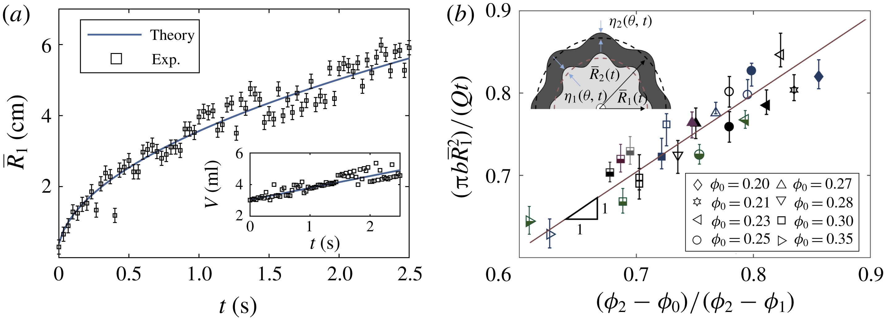
. Figure 2(a) shows the plot of
 $\overline{R}_{1}(t)$
for a single experiment (i.e.
 $\unicode[STIX]{x1D719}_{0}=0.3$
,
 $b=0.76\,\text{mm}$
,
 $Q=150\,\text{ml}~\text{min}^{-1}$
) in reasonable agreement with theory, while the inset shows the volume of the particle band,
 $V=\unicode[STIX]{x1D719}_{2}\unicode[STIX]{x03C0}(\overline{R}_{2}^{2}-\overline{R}_{1}^{2})b$
, grows linearly with
 $t$
. Figure 2(b) provides a comparison of normalised
 $\overline{R}_{1}(t)$
as given in (3.3) for varying
 $\unicode[STIX]{x1D719}_{0}$
,
 $Q$
and
 $b/d$
.
(a) Inner radius as a function of time for
 $\unicode[STIX]{x1D719}_{0}=0.3$
,
 $b=0.77\,\text{mm}$
,
 $d=0.325\,\text{mm}$
and
 $Q=150\,\text{ml}~\text{min}^{-1}$
; the inset shows the linear growth of the particle band volume
 $V$
with time. (b) Verification of the kinematic boundary condition on the inner interface for
 $b/d=1.23$
(blue), 1.92 (black), 2.3 (violet), 3.15 (green), 3.48 (grey) with
 $Q=75\,\text{ml}~\text{min}^{-1}$
(solid),
 $100~\text{ml}~\text{min}^{-1}$
(half solid),
 $150~\text{ml}~\text{min}^{-1}$
(empty), with the schematic for perturbed inner and outer interfaces.

3.3 Linear stability analysis
We decompose the velocity and pressure perturbations into Fourier modes in
 $\unicode[STIX]{x1D703}$
:
 $$\begin{eqnarray}\boldsymbol{u}_{j}^{\prime }=\mathop{\sum }_{n=1}^{\infty }\hat{\boldsymbol{u}}_{j,n}\text{e}^{\text{i}n\unicode[STIX]{x1D703}}+\text{c.c.},\quad p_{j}^{\prime }=\mathop{\sum }_{n=1}^{\infty }\hat{p}_{j,n}\text{e}^{\text{i}n\unicode[STIX]{x1D703}}+\text{c.c.},\end{eqnarray}$$
where the modal amplitudes are functions of radial position and time as
 $\hat{\boldsymbol{u}}_{j,n}=\hat{u} _{r,j,n}(r,t)\hat{\boldsymbol{e}}_{r}+\hat{u} _{\unicode[STIX]{x1D703},j,n}(r,t)\hat{\boldsymbol{e}}_{\unicode[STIX]{x1D703}}$
and
 $\hat{p}_{j}=\hat{p}_{j,n}(r,t)$
; ‘
 $\text{c.c.}$
’ denotes the complex conjugate of the preceding term. Because the governing field equations are linear, Laplace’s equation for pressure also governs the perturbation. The general solution is
 $$\begin{eqnarray}\displaystyle & \displaystyle \hat{p}_{j,n}=A_{j,n}(t)r^{n}+B_{j,n}(t)r^{-n}, & \displaystyle\end{eqnarray}$$
 $$\begin{eqnarray}\displaystyle & \displaystyle \hat{u} _{r,j,n}=-nM_{j}\left(A_{j,n}(t)r^{n-1}-B_{j,n}(t)r^{-(n+1)}\right)\!, & \displaystyle\end{eqnarray}$$
 $$\begin{eqnarray}\displaystyle & \displaystyle \hat{u} _{\unicode[STIX]{x1D703},j,n}=-\text{i}nM_{j}\left(A_{j,n}(t)r^{n-1}+B_{j,n}(t)r^{-(n+1)}\right)\!, & \displaystyle\end{eqnarray}$$
 $j=1$
, and the particle band,
 $j=2$
. We denote the perturbed location of the interface between the low-concentration suspension and the band as
 $R_{1}(\unicode[STIX]{x1D703},t)=\overline{R}_{1}(t)+\unicode[STIX]{x1D702}_{1}(\unicode[STIX]{x1D703},t)$
and the interface between the band and the ambient air as
 $R_{2}(\unicode[STIX]{x1D703},t)=\overline{R}_{2}(t)+\unicode[STIX]{x1D702}_{2}(\unicode[STIX]{x1D703},t)$
, as shown in the inset of figure 2(b). We write the interface perturbations in Fourier series as
 $$\begin{eqnarray}\unicode[STIX]{x1D702}_{j}(\unicode[STIX]{x1D703},t)=\mathop{\sum }_{n=1}^{\infty }\hat{\unicode[STIX]{x1D702}}_{j,n}(t)\text{e}^{\text{i}n\unicode[STIX]{x1D703}}+\text{c.c.},\quad j=1,2.\end{eqnarray}$$
The linearised form of equal normal velocities on
 $R_{1}$
requires
 $$\begin{eqnarray}\hat{u} _{r,1,n}=\hat{u} _{r,2,n}\quad \text{on}~r=\overline{R}_{1}.\end{eqnarray}$$
The absence of surface tension at
 $R_{1}$
requires the normal component of the traction vector on either side of the interface to be equal and opposite. Linearising about
 $\overline{R}_{1}$
gives
 $$\begin{eqnarray}\hat{p}_{1,n}-\hat{p}_{2,n}+2\left(\unicode[STIX]{x1D707}_{2}\frac{\unicode[STIX]{x2202}\hat{u} _{r,2,n}}{\unicode[STIX]{x2202}r}-\unicode[STIX]{x1D707}_{1}\frac{\unicode[STIX]{x2202}\hat{u} _{r,1,n}}{\unicode[STIX]{x2202}r}\right)+\hat{\unicode[STIX]{x1D702}}_{1,n}\left(\frac{\text{d}\overline{p}_{1}}{\text{d}r}-\frac{\text{d}\overline{p}_{2}}{\text{d}r}+2\left(\unicode[STIX]{x1D707}_{2}-\unicode[STIX]{x1D707}_{1}\right)\frac{\text{d}^{2}\overline{u}_{r}}{\text{d}r^{2}}\right)=0,\end{eqnarray}$$
on
 $r=\overline{R}_{1}$
. Finally, the dynamic boundary condition at the suspension–air interface gives a jump in normal traction due to surface tension, which is linearised as
 $$\begin{eqnarray}\hat{p}_{2,n}-2\unicode[STIX]{x1D707}_{2}\frac{\unicode[STIX]{x2202}\hat{u} _{r,2,n}}{\unicode[STIX]{x2202}r}+\hat{\unicode[STIX]{x1D702}}_{2,n}\left(\frac{\text{d}\overline{p}_{2}}{\text{d}r}-2\unicode[STIX]{x1D707}_{2}\frac{\text{d}^{2}\overline{u}_{r}}{\text{d}r^{2}}\right)=\unicode[STIX]{x1D6FE}_{2}\frac{\left(n^{2}-1\right)\hat{\unicode[STIX]{x1D702}}_{2,n}}{\overline{R}_{2}^{2}}\quad \text{on}~r=\overline{R}_{2}.\end{eqnarray}$$
Together with
 $B_{1,n}=0$
to satisfy boundedness as
 $r\rightarrow 0$
, equation (3.7c
) can be solved for the remaining coefficients, in terms of the yet unknown interface disturbances
 $\hat{\unicode[STIX]{x1D702}}_{j,n}(t)$
.
In order to determine the amplitudes of the disturbance of each of the interfaces, we write kinematic boundary conditions for the position of each interface. The kinematic boundary condition at the outer interface can be linearised as
 $$\begin{eqnarray}\frac{\text{d}\hat{\unicode[STIX]{x1D702}}_{2,n}}{\text{d}t}=\hat{u} _{r,2,n}+\frac{\text{d}\overline{u}_{r}}{\text{d}r}\hat{\unicode[STIX]{x1D702}}_{2,n}\quad \text{on}~r=\overline{R}_{2}.\end{eqnarray}$$
Finally, on the inner interface, the volumetric flow rate of particles into the interface is
 $$\begin{eqnarray}q=\int _{0}^{2\unicode[STIX]{x03C0}}\unicode[STIX]{x1D719}_{1}rb\left(\unicode[STIX]{x1D6FD}\boldsymbol{u}_{1}-\frac{\unicode[STIX]{x2202}R_{1}}{\unicode[STIX]{x2202}t}\hat{\boldsymbol{e}}_{r}\right)\boldsymbol{\cdot }\hat{\boldsymbol{n}}_{1}\text{d}\unicode[STIX]{x1D703}\quad \text{on}~r=\overline{R}_{1}+\unicode[STIX]{x1D702}_{1}.\end{eqnarray}$$
The leading-order term in this expression accounts for the net increase in volume of the particle band and is positive when
 $\unicode[STIX]{x1D6FD}>1$
. We define the location of the interface such that its perturbation conserves the volume of particles in the high-concentration band. In other words, the combined effects of the perturbation of the suspension velocity and perturbation of the interface surface area result in zero change in the volume of the particle band. Setting the first-order correction term in the integrand to zero yields
 $$\begin{eqnarray}\frac{\text{d}\hat{\unicode[STIX]{x1D702}}_{1,n}}{\text{d}t}=\frac{1}{\overline{R}_{1}}\left[\unicode[STIX]{x1D6FD}\left(\overline{R}_{1}\hat{u} _{r,1,n}+\hat{\unicode[STIX]{x1D702}}_{1,n}\left(\overline{R}_{1}\frac{\text{d}\overline{u}_{r}}{\text{d}r}+\overline{u}_{r}\right)\right)-\hat{\unicode[STIX]{x1D702}}_{1,n}\frac{\text{d}\overline{R}_{1}}{\text{d}t}\right]\quad \text{on}~r=\overline{R}_{1}\end{eqnarray}$$
as the kinematic boundary condition for the position of the inner interface. Since the perturbed velocities,
 $\hat{u} _{r,j,n}$
, are already found in terms of
 $\hat{\unicode[STIX]{x1D702}}_{j,n}$
using (3.5), (3.7) and
 $B_{1,n}=0$
, the two kinematic boundary conditions provide a linear system of equations for the growth of the disturbance of each interface. For a given wavenumber
 $n$
, the governing equations for
 $\hat{\unicode[STIX]{x1D702}}_{1,n}$
and
 $\hat{\unicode[STIX]{x1D702}}_{2,n}$
are coupled with non-constant coefficients:
 $$\begin{eqnarray}\frac{\text{d}\hat{\unicode[STIX]{x1D702}}_{j,n}}{\text{d}t}=\mathop{\sum }_{k=1}^{2}\unicode[STIX]{x1D60E}_{jk,n}(t)\hat{\unicode[STIX]{x1D702}}_{k,n},\quad j=1,2;\quad n=1,2,3,\ldots\end{eqnarray}$$
where the growth matrix
 $\unicode[STIX]{x1D60E}_{jk,n}(t)$
is a time-varying matrix of rank two. In this two-dimensional linear system,
 $\unicode[STIX]{x1D60E}_{jk,n}(t)$
has two eigenvalues
 $\unicode[STIX]{x1D706}_{i,n}(t)$
for each wavenumber
 $n$
, where the larger eigenvalue,
 $\unicode[STIX]{x1D706}_{1,n}$
, is the growth rate for the in-phase mode and the smaller eigenvalue,
 $\unicode[STIX]{x1D706}_{2,n}$
, corresponds to the out-of-phase mode of deformation. Notably,
 $\unicode[STIX]{x1D60E}_{jk,n}(t)$
is not diagonal, meaning that the growth of a disturbance on the inner, intrinsically unstable miscible interface at
 $R_{1}$
must be coupled to the growth of a disturbance on the outer interface at
 $R_{2}$
. The coupling between the two interfaces is the key mechanism through which the stabilising effects of surface tension can damp high-wavenumber perturbations at the miscible interface. In the same manner, this coupling allows the destabilising jump in effective viscosity at
 $R_{1}$
to drive the instability at
 $R_{2}$
. The full expression for
 $\unicode[STIX]{x1D60E}_{jk,n}$
is included in supplementary material (available at https://doi.org/10.1017/jfm.2019.239).
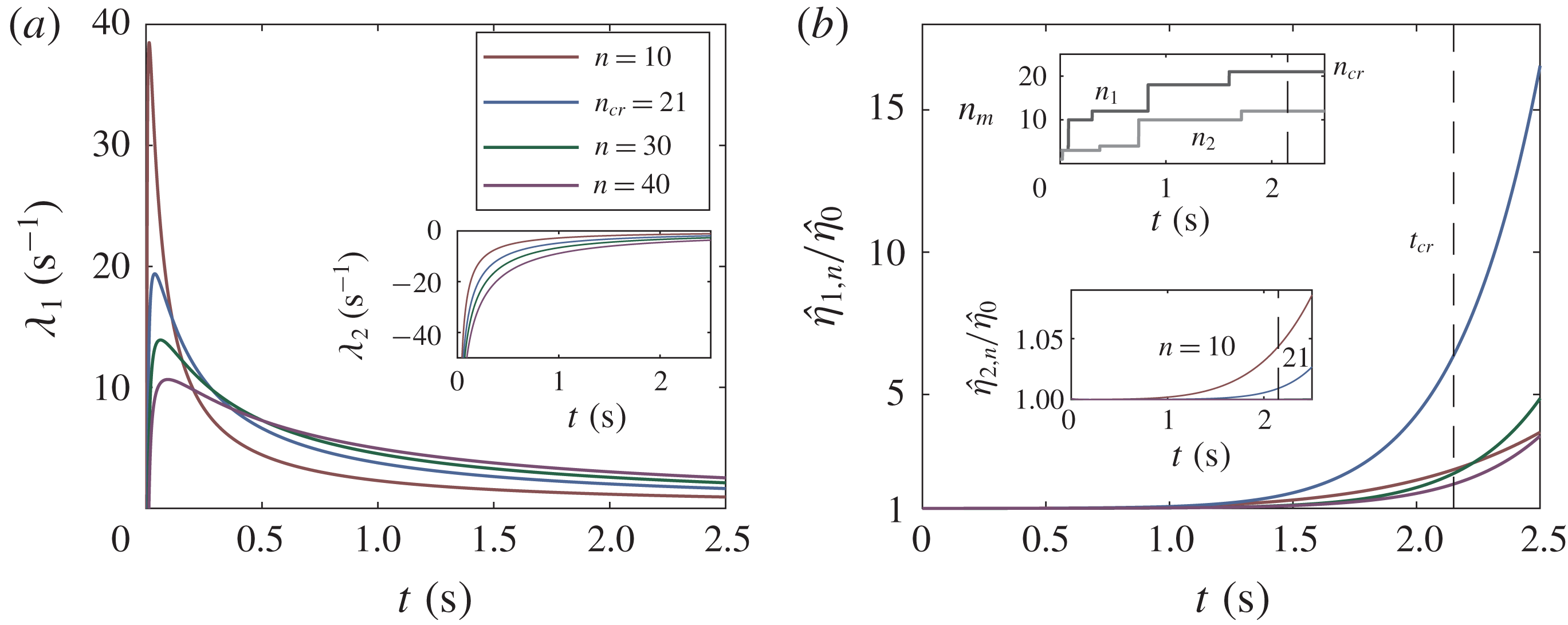
Theoretically predicted growth rate and amplitude of disturbances for
 $\unicode[STIX]{x1D719}_{0}=0.3$
,
 $b=0.96~\text{mm}$
,
 $Q=100~\text{ml}~\text{min}^{-1}$
,
 $V_{0}=2.89~\text{ml}$
. (a) Larger eigenvalue of the growth matrix,
 $\unicode[STIX]{x1D706}_{1,n}$
, for four wavenumbers. The inset shows the smaller eigenvalue of the growth matrix,
 $\unicode[STIX]{x1D706}_{2,n}$
, which is negative, for each of these wavenumbers. (b) The modal amplitudes obtained by integration of (3.11). The primary plot gives the modal amplitudes of the disturbance of the inner interface,
 $\hat{\unicode[STIX]{x1D702}}_{1,n}$
. The top inset gives the wavenumbers with the largest amplitude,
 $n_{m}=\text{arg}\,\text{max}\hat{\unicode[STIX]{x1D702}}_{n}$
. The lower inset gives the amplitudes of the disturbance of the outer immiscible interface, whose change is an order of magnitude smaller than that of the inner miscible interface.

4 Results
The eigenvalues for several modes are plotted versus time in figure 3(a), based on the empirical expression for the effective viscosity by Morris & Boulay (Reference Morris and Boulay1999), or
 $\unicode[STIX]{x1D707}(\unicode[STIX]{x1D719})/\unicode[STIX]{x1D707}_{l}=1+2.5\unicode[STIX]{x1D719}_{m}^{2}/(\unicode[STIX]{x1D719}_{m}-\unicode[STIX]{x1D719})+0.1\unicode[STIX]{x1D719}^{2}/(\unicode[STIX]{x1D719}_{m}-\unicode[STIX]{x1D719})^{2}$
, with
 $\unicode[STIX]{x1D719}_{m}=0.64$
. It is important to note that the qualitative results of our analysis are not affected by the particular choice of
 $\unicode[STIX]{x1D707}(\unicode[STIX]{x1D719})$
, as demonstrated by the sensitivity analysis in the appendix. The primary plot in figure 3(a) contains the larger, unstable eigenvalues,
 $\unicode[STIX]{x1D706}_{1,n}$
, and the inset shows the smaller, stable eigenvalues,
 $\unicode[STIX]{x1D706}_{2,n}$
. The results show that small-wavenumber disturbances are most unstable at early times, as stabilising surface tension on the outer interface is large when the outer radius of curvature is small. At later times, the stabilising effect of surface tension is reduced with the larger radius of curvature. This results in high-wavenumber modes becoming less stable, characteristic of traditional miscible viscous fingering. Additionally, magnitudes of all growth rates decrease over time because the fluid velocity at the interfaces decreases as it flows radially outwards from the source.
As evident in figure 3(a), the eigenvalues (and eigenvectors) evolve with time due to the time-dependent nature of
 $\overline{R}_{1}(t)$
and
 $\overline{R}_{2}(t)$
. Therefore, treating the wavenumber with the largest instantaneous growth rate as the critical wavenumber does not properly incorporate the temporal evolution of the growth rates. Instead, we numerically integrate (3.11) to find the wavenumber with the largest amplitude at any instant in time, as suggested by Cardoso & Woods (Reference Cardoso and Woods1995). Assuming the initial amplitudes of all wavenumbers are identical (
 $\hat{\unicode[STIX]{x1D702}}_{j,n}(t_{0})=\hat{\unicode[STIX]{x1D702}}_{0}$
, where
 $\hat{\unicode[STIX]{x1D702}}_{0}$
is set to
 $b$
), we integrate from
 $t_{0}$
such that
 $\overline{R}_{1}(t_{0})=d_{hole}/2$
to obtain
 $\hat{\unicode[STIX]{x1D702}}_{1,n}(t)$
and
 $\hat{\unicode[STIX]{x1D702}}_{2,n}(t)$
, as shown in figure 3(b). The largest-amplitude Fourier mode,
 $n_{m}$
, corresponds to a wavenumber with the largest integrated growth rate. The upper inset of figure 3(b) shows that
 $n_{m}$
does not change appreciably over the time scale of interest for the experiments, and the lower subplot shows that the growth in
 $\hat{\unicode[STIX]{x1D702}}_{2,n}$
is an order of magnitude smaller than that in
 $\hat{\unicode[STIX]{x1D702}}_{1,n}$
for typical wavenumbers.
In order to extract the critical wavenumber
 $n_{cr}$
, we numerically compute a critical time
 $t_{cr}$
, which is intended to represent the experimental criterion that the low-concentration suspension reaches the suspension–air interface (i.e. the particle band breaks) at
 $t_{cr}$
. In the model, the perturbed inner interface must reach the position of the perturbed outer interface at the critical time, giving the following implicit equation for
 $t_{cr}$
:
 $$\begin{eqnarray}\sup \{|\hat{\unicode[STIX]{x1D702}}_{1,n}(t_{cr})|-|\hat{\unicode[STIX]{x1D702}}_{2,n}(t_{cr})|\mid n=1,2,3,\cdots \!\,\}=\overline{R}_{2}(t_{cr})-\overline{R}_{1}(t_{cr}).\end{eqnarray}$$
The amplitudes are subtracted because the most unstable mode at any wavenumber is the mode in which the inner and outer interface perturbations are in phase. Among different characteristic length scales present in the problem (for example,
 $d$
,
 $b$
), we find that
 $\hat{\unicode[STIX]{x1D702}}_{0}=b$
yields the values of
 $t_{cr}$
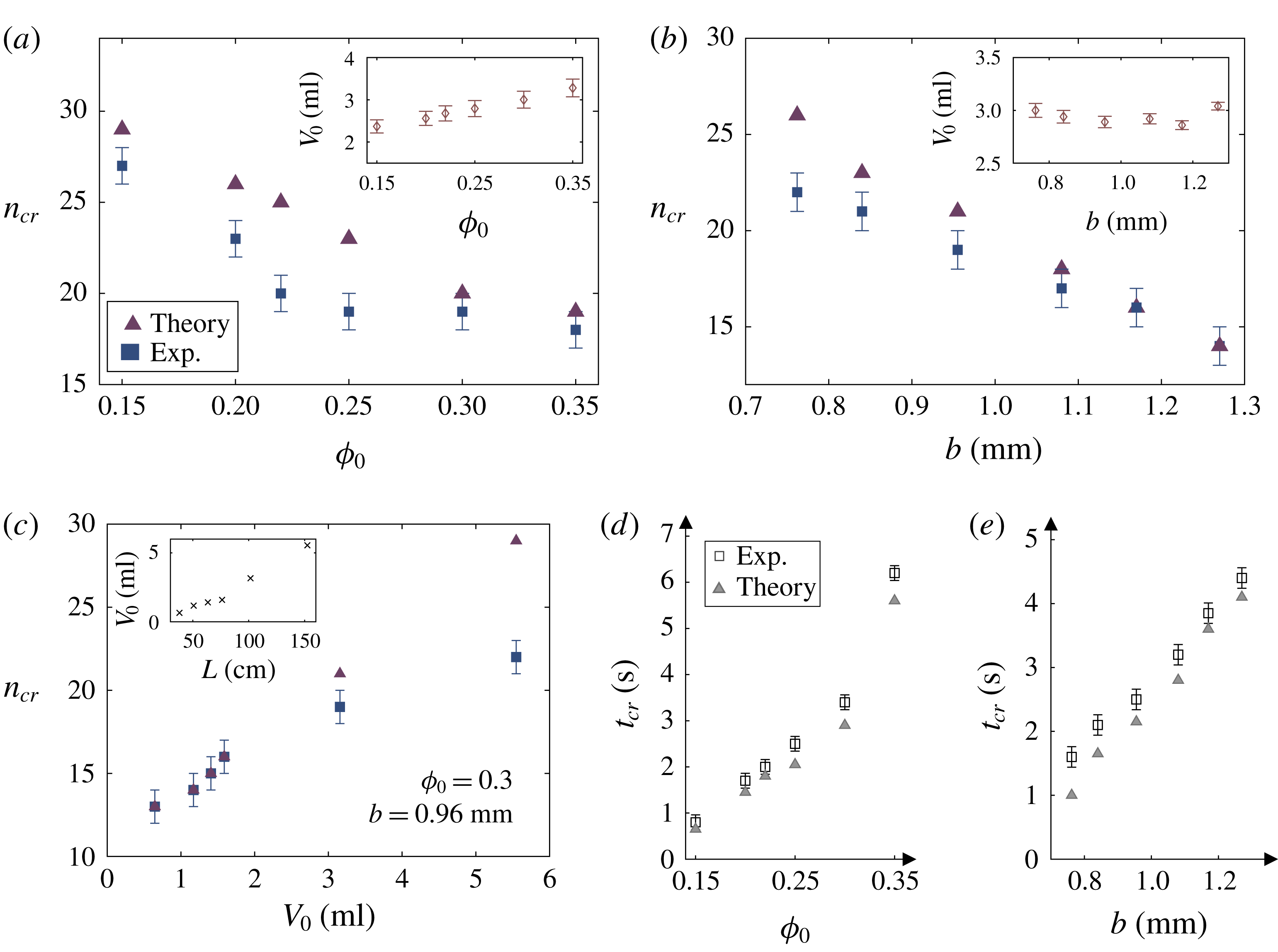
that most reasonably match the experiments, as shown in figure 4(d,e). However, it is important to recognise that the linear theory breaks down as
 $|\hat{\unicode[STIX]{x1D702}}_{1,n}|$
becomes comparable to the inner radius and nonlinear effects become important. As previously demonstrated by Cardoso & Woods (Reference Cardoso and Woods1995), linear theory provides an analytically tractable formulation to describe the initial growth of the instability and is representative of some of the weakly nonlinear behaviour. In the cases where the band thickness is small and the amplitude of disturbance is still small at
 $t_{cr}$
, we expect our formulation to be reasonably predictive. However, when the band thickness is large, necessitating large-amplitude disturbances to realise the criterion for
 $t_{cr}$
in (4.1), our model fails to incorporate all the physics required to make accurate predictions of
 $t_{cr}$
and the corresponding modal amplitudes. Weakly nonlinear theory or fully numeric nonlinear simulations are required to understand the entire picture at that point.
Finally,
 $n_{cr}=\text{arg}\,\text{max}\hat{\unicode[STIX]{x1D702}}_{1,n}(t_{cr})$
corresponds to the wavenumber with the largest amplitude at
 $t_{cr}$
. We note that different values of
 $\hat{\unicode[STIX]{x1D702}}_{0}$
result in different values of
 $t_{cr}$
and, therefore,
 $n_{cr}$
. However, the qualitative variations in
 $n_{cr}$
remain unaffected by our choice of
 $\hat{\unicode[STIX]{x1D702}}_{0}$
. Figure 4(a,b) compares the theoretically predicted and experimentally observed critical wavenumbers in the parametric studies of
 $\unicode[STIX]{x1D719}_{0}$
and
 $b$
. Here, the experimental value of
 $V_{0}$
(as shown in the inset) is used as an empirical input to the theory. As shown in figure 4(c), we additionally vary
 $V_{0}$
, by modulating the tube length
 $L$
while fixing
 $\unicode[STIX]{x1D719}_{0}=0.3$
and
 $b=0.96~\text{mm}$
; this allows us to isolate the effects of the initial band thickness (i.e.
 $\bar{R}_{2}(t=0)=\sqrt{V_{0}/(\unicode[STIX]{x03C0}b)}$
) on the critical wavenumber. Overall, theoretical values of
 $n_{cr}$
are in good qualitative agreement with the experiments, correctly capturing the gradual decrease in
 $n_{cr}$
with increasing
 $\unicode[STIX]{x1D719}_{0}$
and
 $b$
, respectively, while
 $n_{cr}$
increases with
 $V_{0}$
. The systematic error between theory and experiments may be attributed to the omission of the nonlinear terms. In particular, the notable deviation between theory and experiments for large
 $V_{0}$
in figure 4(c) suggests that the nonlinear terms dominate as the perturbations grow large enough to break through the thick band.
The results of the parametric studies can be interpreted in light of the fundamental competition between the destabilising viscosity gradient on the inner interface and the stabilising surface tension on the outer interface. In figure 4(a), increasing
 $\unicode[STIX]{x1D719}_{0}$
gives a corresponding increase in
 $\unicode[STIX]{x1D719}_{1}$
and
 $\unicode[STIX]{x1D707}_{1}$
. This increase in
 $\unicode[STIX]{x1D719}_{1}$
, while fixing
 $\unicode[STIX]{x1D719}_{2}$
and
 $\unicode[STIX]{x1D707}_{2}$
, decreases the destabilising viscosity gradient at the inner interface and causes all wavenumbers to grow more slowly. Thus wavenumbers that are marginally unstable with a large viscosity gradient become stable as the viscosity gradient decreases, and only small wavenumbers remain unstable, resulting in a decrease in
 $n_{cr}$
.
Comparison of experimentally observed critical wavenumber with the theoretical prediction for (a) varying
 $\unicode[STIX]{x1D719}_{0}$
at
 $b=1.02~\text{mm}$
, (b) varying
 $b$
at
 $\unicode[STIX]{x1D719}_{0}=0.3$
, and (c) varying
 $V_{0}$
, while
 $b=0.96~\text{mm}$
and
 $\unicode[STIX]{x1D719}_{0}=0.3$
. Comparison of experimentally observed critical time for band breakup with the theoretical prediction for (d) varying
 $\unicode[STIX]{x1D719}_{0}$
at
 $b=1.02~\text{mm}$
and (e) varying
 $b$
with
 $\unicode[STIX]{x1D719}_{0}=0.3$
. For all cases,
 $Q=100~\text{ml}~\text{min}^{-1}$
.

Figure 4(b) shows that increasing
 $b$
also results in a decrease in
 $n_{cr}$
. As
 $b$
increases while
 $V_{0}$
is unaltered, the band thickness,
 $\overline{R}_{2}-\overline{R}_{1}$
, must decrease. This decrease in band thickness brings the outer interface closer to the unstable inner interface, enhancing the effects of surface tension and eliminating the high-wavenumber disturbances. By the same token, increasing
 $V_{0}$
, and hence the initial band thickness, must lessen the effect of surface tension and result in larger
 $n_{cr}$
, as shown in figure 4(c). Overall, the simple analysis demonstrates that surface tension on the outer interface can stabilise the inner miscible interface, as the disturbances on the two interfaces become coupled in (3.11).
5 Summary and conclusions
In summary, we have run series of experiments and conducted a linear stability analysis of the radial suspension flow in a Hele-Shaw cell, for varying
 $\unicode[STIX]{x1D719}_{0}$
,
 $b$
and
 $V_{0}$
. We extract the evolution of the particle band thickness over time as well as the critical wavenumber
 $n_{cr}$
upon the band breakup. To rationalise the experimental observations, the model incorporates the destabilising effect of low-concentration suspension displacing high-concentration suspension and the stabilising effect of surface tension on the suspension–air interface. Unlike the work of Cardoso & Woods (Reference Cardoso and Woods1995), our system contains a miscible interface between the low-concentration and high-concentration suspensions, for which we posit a kinematic boundary condition based on particle flux.
The main result of this paper is to model the coupling between the unstable miscible interface and the inherently stable immiscible interface, which yields the observed finite wavenumber of the particle band breaking. The model reasonably predicts the value of
 $n_{cr}$
from the experiments, by qualitatively capturing the decrease in
 $n_{cr}$
with
 $\unicode[STIX]{x1D719}_{0}$
and
 $b$
and the increase with
 $V_{0}$
. In addition, we are able to theoretically model the temporal evolution of the high-concentration suspension band and the critical time
 $t_{cr}$
at which the band breaks, despite the breakdown of the linear theory near
 $t_{cr}$
.
Future work includes employing the weakly nonlinear theory or fully nonlinear simulations, in lieu of linear stability. The current analysis could also benefit from the use of better models for particle transport in the
 $z$
-direction in the limit as
 $b$
approaches
 $d$
, and an improved constitutive model for the suspension in this same limit. For instance, instead of treating the suspension as a simple Newtonian fluid with enhanced viscosity, the high-concentration particle band may be modelled as a non-Newtonian fluid with a finite yield stress to simulate its solid-like properties. Ideally these improved models would be compared with fully computational analysis for verification.
Supplementary material
Supplementary material is available at https://doi.org/10.1017/jfm.2019.239.
Acknowledgements
We acknowledge Dr F. Xu for valuable discussions and for providing raw data for figure 2(b). This work was sponsored by the National Science Foundation through the University of Minnesota MRSEC (DMR-1420013) and the grant (CBET-1839103).
Appendix. Sensitivity analysis
In order to test the robustness of our results, the stability analysis is repeated for
 $\unicode[STIX]{x1D719}_{2}=0.5$
and
 $0.55$
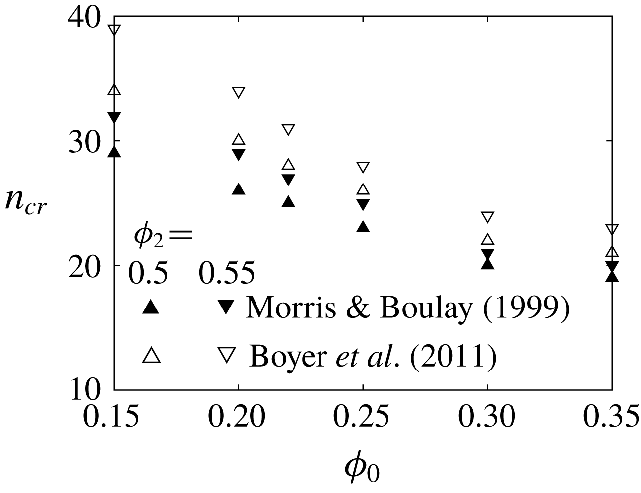
, while we employ the suspension viscosity expressions by Morris & Boulay (Reference Morris and Boulay1999) and by Boyer, Guazzelli & Pouliquen (Reference Boyer, Guazzelli and Pouliquen2011), respectively. The resultant plot of
 $n_{cr}$
versus
 $\unicode[STIX]{x1D719}_{0}$
in figure 5 shows an increase in
 $n_{cr}$
with
 $\unicode[STIX]{x1D719}_{2}=0.55$
, while the use of
 $\unicode[STIX]{x1D707}(\unicode[STIX]{x1D719})$
by Boyer et al. (Reference Boyer, Guazzelli and Pouliquen2011) consistently yields larger
 $n_{cr}$
than that by Morris & Boulay (Reference Morris and Boulay1999) and deviates more from the experimental results. Note that
 $\unicode[STIX]{x1D707}(\unicode[STIX]{x1D719})$
by Boyer et al. (Reference Boyer, Guazzelli and Pouliquen2011) predicts a sharper increase in viscosity with
 $\unicode[STIX]{x1D719}$
. However, the qualitative behaviour of
 $n_{cr}$
remains unchanged between different values of
 $\unicode[STIX]{x1D719}_{2}$
and
 $\unicode[STIX]{x1D707}(\unicode[STIX]{x1D719})$
.
Critical wavenumber as a function of
 $\unicode[STIX]{x1D719}_{0}$
for two different values of
 $\unicode[STIX]{x1D719}_{2}=0.5$
( △ ),
 $\unicode[STIX]{x1D719}_{2}=0.55$
( ▽ ), and two different empirical expressions for
 $\unicode[STIX]{x1D707}(\unicode[STIX]{x1D719})$
by Morris & Boulay (Reference Morris and Boulay1999) (solid) and Boyer et al. (Reference Boyer, Guazzelli and Pouliquen2011) (empty).