1 Introduction
As is well known, strong stratification and rotation are the key ingredients of the geophysical fluid dynamics underlying atmospheric and oceanic flows. In general, such flows involve a complex intermingling of fast inertia–gravity waves on top of a much slower evolving balanced vortical flow. That balanced flow is essentially controlled by the three-dimensional spatial distribution of the Rossby–Ertel potential vorticity (PV), which is a scalar material invariant in idealized flow and therefore evolves relatively slowly (e.g. Charney Reference Charney1971; Salmon Reference Salmon1982). Dispersive inertia–gravity waves, on the other hand, evolve quickly and can propagate rapidly, especially in the vertical, and this time scale separation leads to the familiar stiffness of the governing equations of motion. Whilst the linear aspects of this scenario are well understood, its nonlinear and turbulent aspects continue to challenge simple understanding, and controversy persists even in the interpretation of very well established observational facts. An example of this is the atmospheric Nastrom–Gage spectrum (Nastrom & Gage Reference Nastrom and Gage1985), which has a scaling behaviour that differs from both three-dimensional (Kolmogorov Reference Kolmogorov1941) and two-dimensional (Kraichnan Reference Kraichnan1982) turbulence. Many theories to explain this spectrum have been proposed, among them are versions of two-dimensional turbulence (Lilly Reference Lilly1989; Lindborg Reference Lindborg1999), quasi-geostrophic (QG) theory (Tung & Orlando Reference Tung and Orlando2003), its surface version (Tulloch & Smith Reference Tulloch and Smith2006, Reference Tulloch and Smith2009), stratified turbulence (Lindborg Reference Lindborg2006), rotating stratified turbulence (Lindborg Reference Lindborg2005; Deusebio, Vallgren & Lindborg Reference Deusebio, Vallgren and Lindborg2013) and explanations based on superpositions of QG motions at large scales and internal gravity waves at small scales (e.g. Dewan Reference Dewan1979; Bühler, Callies & Ferrari Reference Bühler, Callies and Ferrari2014; Callies, Ferrari & Bühler Reference Callies, Ferrari and Bühler2014; Callies, Bühler & Ferrari Reference Callies, Bühler and Ferrari2016). Still, controversies persist and a unifying theoretical framework is lacking.
One approach has been to focus on the nonlinear dynamics of the fast inertia–gravity waves whilst ignoring the PV distribution. Methods in this approach can be borrowed, for example, from weak turbulence theory (Majda, McLaughlin & Tabak Reference Majda, McLaughlin and Tabak1997; Nazarenko Reference Nazarenko2011; Zakharov, L’vov & Falkovich Reference Zakharov, L’vov and Falkovich2012), or large-magnitude critical balance theory (e.g. Nazarenko & Schekochihin Reference Nazarenko and Schekochihin2011). Such an approach would be natural in the context of small-scale oceanic internal waves, for example, which are believed to contribute significantly to downscale energy fluxes and vertical diffusion in the deep ocean (e.g. Wunsch & Ferrari Reference Wunsch and Ferrari2004). Complementary to such wave-centred studies are investigations such as that of Vallgren & Lindborg (Reference Vallgren and Lindborg2010), which focuses entirely on the slow balanced vortical component. Other research concerns wave–vortex decompositions applied in simulations of the full rotating stratified system in order to distinguish the effects from different components and to study their interactions (Bartello Reference Bartello1995; Smith & Waleffe Reference Smith and Waleffe2002; Deusebio et al. Reference Deusebio, Vallgren and Lindborg2013; Hernandez-Duenas, Smith & Stechmann Reference Hernandez-Duenas, Smith and Stechmann2014; Marino et al. Reference Marino, Rosenberg, Herbert and Pouquet2015b ; Oks et al. Reference Oks, Mininni, Marino and Pouquet2017). Idealized studies of rotating stratified fluid turbulence per se have illuminated questions about the direction of spectral fluxes of energy and enstrophy (where applicable) in numerical simulations. This is a subtle question. For example, Bartello (Reference Bartello1995), Métais et al. (Reference Métais, Bartello, Garnier, Riley and Lesieur1996), Kurien, Wingate & Taylor (Reference Kurien, Wingate and Taylor2008), Marino et al. (Reference Marino, Mininni, Rosenberg and Pouquet2013), Dritschel & McKiver (Reference Dritschel and McKiver2015) report inverse cascades of energy whereas in Marino, Pouquet & Rosenberg (Reference Marino, Pouquet and Rosenberg2015a ), Pouquet et al. (Reference Pouquet, Marino, Mininni and Rosenberg2017) energy transfers in both directions are found to co-exist, and the dependence of the strength of upscale and downscale energy transfer on the Prandtl ratio is studied. Presumably, the last word has not been spoken yet in this area.
In our opinion, a promising tool in this situation is the classical Kármán–Howarth–Monin (KHM) equation (cf. Kolmogorov Reference Kolmogorov1941; Monin & Yaglom Reference Monin and Yaglom1975), which initially described how measurable third-order structure functions can be linked to inertial-range energy fluxes in three-dimensional isotropic turbulence. Related theories for inertial ranges have since been developed for two-dimensional turbulence (Bernard Reference Bernard1999; Lindborg Reference Lindborg1999; Yakhot Reference Yakhot1999; Cerbus & Chakraborty Reference Cerbus and Chakraborty2017), turbulence with helicity (Chkhetiani Reference Chkhetiani1996; Gomez, Politano & Pouquet Reference Gomez, Politano and Pouquet2000; Kurien Reference Kurien2003), QG flow (Lindborg Reference Lindborg2007), stratified flow (Augier, Galtier & Billant Reference Augier, Galtier and Billant2012) and rotating stratified flow (Lindborg & Cho Reference Lindborg and Cho2000; Cho & Lindborg Reference Cho and Lindborg2001; Lindborg & Cho Reference Lindborg and Cho2001; Kurien, Smith & Wingate Reference Kurien, Smith and Wingate2006; Deusebio, Augier & Lindborg Reference Deusebio, Augier and Lindborg2014a ). Our own recent work in Xie & Bühler (Reference Xie and Bühler2018) showed how to extend these inertial-range theories to cover the entire non-dissipative range of scales, including the forcing scales. However, rotating stratified turbulence is typically strongly anisotropic, and so far diagnostic relations between structure functions and energy fluxes for anisotropic flows have not been derived yet without the need for ad hoc closure assumptions. This is the theoretical bottleneck we are facing today: developing third-order structure function theory to the point where it becomes directly applicable to rotating and stratified flows.
In the present paper, we are seeking to make progress on this problem by making three severe simplifying assumptions that lead to a solvable model problem. First, we are restricting to inertia–gravity wave turbulence by keeping the PV equal to its undisturbed background value throughout the domain. By definition, this eliminates any PV-controlled balanced flow. Second, we restrict the fluid dynamics to a two-dimensional vertical slice domain with periodic boundary conditions. Because of Coriolis forces, the velocity field in this model is still three-dimensional even though the flow variables depend only on two spatial coordinates. This allows for simple numerical simulation as well as easy access to forcing fields that do not project onto the PV even at the nonlinear level. Third, and most peculiarly, we study a setting in which the Coriolis frequency equals the buoyancy frequency. We are not aware of any direct practical application of this setting in atmospheric or ocean flows, rather we pursue it because it offers a radical simplification of the dynamical situation, as it can be shown that the resulting rotating stratified dynamics is isotropic in the vertical plane. This fact, which is not immediately obvious from the governing equations, then allows the machinery of classical isotropic turbulence theory to be applied to this wave system. Thus, we obtain a solvable isotropic wave turbulence toy model, which yields a number of explicit and exact results about energy fluxes and structure functions that are not available in the general case of unequal Coriolis and buoyancy frequencies. For example, the Coriolis effect in the present two-dimensional model is distinct from that in a three-dimensional system, where columnar cyclonic vortices are observed in experiments and numerical simulations (e.g. Biferale et al. Reference Biferale, Bonaccorso, Mazzitelli, van Hinsberg, Lanotte, Musacchio, Perlekar and Toschi2016). Of course, a future complete theory of rotating stratified turbulence should recover our results as a special limiting case. We therefore hope that our results in this paper will stimulate further research into the structure function approach to rotating stratified turbulence.
The structure of the paper is as follows: § 2 gives the governing equations, § 3 contains a heuristic argument for a downscale cascade, § 4 provides the third-order structure function theory, § 5 contains numerical simulations and in § 6 the structure function theory is applied to an idealized three-scale forcing example. Finally, concluding remarks are offered in § 7.
2 Governing equations
The unforced inviscid two-dimensional rotating stratified Boussinesq fluid equations in the vertical
 $xz$
-plane are obtained from the three-dimensional equations by setting
 $\unicode[STIX]{x2202}_{y}=0$
, which yields
 $$\begin{eqnarray}\displaystyle & \displaystyle u_{t}+uu_{x}+wu_{z}-fv=-p_{x}, & \displaystyle\end{eqnarray}$$
 $$\begin{eqnarray}\displaystyle & \displaystyle v_{t}+uv_{x}+wv_{z}+fu=0, & \displaystyle\end{eqnarray}$$
 $$\begin{eqnarray}\displaystyle & \displaystyle w_{t}+uw_{x}+ww_{z}-b=-p_{z}, & \displaystyle\end{eqnarray}$$
 $$\begin{eqnarray}\displaystyle & \displaystyle b_{t}+ub_{x}+wb_{z}+N^{2}w=0, & \displaystyle\end{eqnarray}$$
 $$\begin{eqnarray}\displaystyle & \displaystyle u_{x}+w_{z}=0. & \displaystyle\end{eqnarray}$$
 $u$
,
 $v$
and
 $w$
are velocity fields in the
 $x$
,
 $y$
and
 $z$
directions, respectively,
 $b$
is the buoyancy,
 $f$
is the Coriolis frequency and
 $N$
is the buoyancy (Brunt–Väisälä) frequency. Both frequencies are assumed constant. Now, as is well known, the buoyancy equation is equivalent to the materially invariance of a vertical stratification variable
 $$\begin{eqnarray}\displaystyle S=N^{2}z+b, & & \displaystyle\end{eqnarray}$$
say, a fact that also holds in the three-dimensional case. However, in the present two-dimensional case the same interpretation can also be given for the
 $y$
-component of the momentum equation, which expresses the material invariance of
 $$\begin{eqnarray}\displaystyle M=f^{2}x+fv. & & \displaystyle\end{eqnarray}$$
This new field
 $M$
can be viewed as a horizontal stratification and indeed the field
 $fv$
enters the
 $x$
-momentum equation in the same way as the buoyancy
 $b$
enters the
 $z$
-momentum equation. Thus, we have a pair of buoyancy type fields
 $fv$
and
 $b$
and if
 $f=N$
this will enable us to construct an isotropic system (shown in § 2.1). Hereafter we call
 $u$
and
 $w$
the in-plane velocities, or velocities for simplicity, and refer to
 $fv$
and
 $b$
as buoyancy scalars. A similar viewpoint is adopted in the astrophysical context, where the background rotation contributes to the angular momentum stratification (cf. Knobloch Reference Knobloch1982).
The Rossby–Ertel PV of the system (2.1) can be expressed as the Jacobian between
 $M$
and
 $S$
, i.e.
 $$\begin{eqnarray}\displaystyle q={\displaystyle \frac{1}{fN^{2}}}\,J(M,S)=f+v_{x}+{\displaystyle \frac{fb_{z}}{N^{2}}}+(v_{x}b_{z}-v_{z}b_{x}){\displaystyle \frac{1}{N^{2}}}. & & \displaystyle\end{eqnarray}$$
This yields a peculiar geometric interpretation of
 $q$
in the present two-dimensional case: it measures the area content of the curvilinear coordinate mesh induced by the advected fields
 $M$
and
 $S$
. In this interpretation
 $q$
is materially invariant because the flow is area-preserving in the
 $xz$
-plane. We will assume throughout that the PV is equal to its background value, i.e.
 $$\begin{eqnarray}\displaystyle q=f\quad \Leftrightarrow \quad v_{x}+{\displaystyle \frac{fb_{z}}{N^{2}}}+(v_{x}b_{z}-v_{z}b_{x}){\displaystyle \frac{1}{N^{2}}}=0. & & \displaystyle\end{eqnarray}$$
Notably, the in-plane velocity field
 $(u,w)$
makes no contribution to
 $q$
and is hence purely wave related. The precise association of these velocity components with the waves does not hold in three-dimensional flow, and it is the key to forcing only the wave field later on. The total energy preserved by (2.1) is
 $$\begin{eqnarray}\displaystyle {\mathcal{E}}_{tot}={\displaystyle \frac{1}{2}}\int \left(u^{2}+w^{2}+{\displaystyle \frac{1}{f^{2}}}(fv)^{2}+{\displaystyle \frac{1}{N^{2}}}b^{2}\right)\text{d}x\,\text{d}z, & & \displaystyle\end{eqnarray}$$
where we highlighted the functional similarity of
 $fv$
and
 $b$
. The linear dispersion relation for inertia–gravity waves is
 $$\begin{eqnarray}\displaystyle \unicode[STIX]{x1D714}^{2}={\displaystyle \frac{N^{2}k^{2}+f^{2}m^{2}}{k^{2}+m^{2}}}, & & \displaystyle\end{eqnarray}$$
where
 $\unicode[STIX]{x1D714}$
is the frequency, and
 $k$
and
 $m$
are the horizontal and vertical wavenumbers, respectively. The third eigenvector of the linearized system has zero frequency and describes the balanced vortical flow component, which satisfies
 $$\begin{eqnarray}\displaystyle u=w=0,\quad fv=p_{x},\quad b=p_{z},\quad \text{and}\quad p_{xx}+{\displaystyle \frac{f^{2}}{N^{2}}}p_{zz}=f(q-f). & & \displaystyle\end{eqnarray}$$
These steady linear states are in fact steady in the nonlinear system as well, which is another aspect of the two-dimensional situation that does not hold for three-dimensional flow. For us the balanced state will be zero throughout because of (2.5).
2.1 Isotropic system if
 $f=N$

In the peculiar special case
 $f=N$
the exact rotating stratified two-dimensional dynamics is isotropic in the
 $xz$
-plane, but this fact is not immediately obvious from the equations. A hint that this is true comes from the linear dispersion relation (2.7), which for
 $f=N$
reduces to the monochromatic
 $\unicode[STIX]{x1D714}^{2}=N^{2}$
for all wavenumbers
 $(k,m)$
. Here we show that this isotropy also holds for the full nonlinear dynamics. First, by defining
 $\unicode[STIX]{x1D703}=b/N$
we rewrite (2.1) in the more symmetric form
 $$\begin{eqnarray}\displaystyle & \displaystyle u_{t}+uu_{x}+wu_{z}-fv=-p_{x}, & \displaystyle\end{eqnarray}$$
 $$\begin{eqnarray}\displaystyle & \displaystyle v_{t}+uv_{x}+wv_{z}+fu=0, & \displaystyle\end{eqnarray}$$
 $$\begin{eqnarray}\displaystyle & \displaystyle w_{t}+uw_{x}+ww_{z}-N\unicode[STIX]{x1D703}=-p_{z}, & \displaystyle\end{eqnarray}$$
 $$\begin{eqnarray}\displaystyle & \displaystyle \unicode[STIX]{x1D703}_{t}+u\unicode[STIX]{x1D703}_{x}+w\unicode[STIX]{x1D703}_{z}+Nw=0, & \displaystyle\end{eqnarray}$$
 $$\begin{eqnarray}\displaystyle & \displaystyle u_{x}+w_{z}=0. & \displaystyle\end{eqnarray}$$
 $f=N$
then time can be rescaled by the common time scale
 $1/f=1/N$
, which sets both
 $N$
and
 $f$
to unity in (2.9) and therefore
 $\unicode[STIX]{x1D714}^{2}=1$
in (2.7). Note also that
 $M=x+v$
and
 $S=z+\unicode[STIX]{x1D703}$
in this scaling. Introducing a streamfunction
 $\unicode[STIX]{x1D713}$
such that
 $(u,\,w)=\unicode[STIX]{x1D735}^{\bot }\unicode[STIX]{x1D713}$
with
 $\unicode[STIX]{x1D735}^{\bot }=(-\unicode[STIX]{x2202}_{z},\,\unicode[STIX]{x2202}_{x})$
yields
 $$\begin{eqnarray}\displaystyle & \displaystyle \unicode[STIX]{x1D6FB}^{2}\unicode[STIX]{x1D713}_{t}+J(\unicode[STIX]{x1D713},\unicode[STIX]{x1D6FB}^{2}\unicode[STIX]{x1D713})-\unicode[STIX]{x1D703}_{x}+v_{z}=0, & \displaystyle\end{eqnarray}$$
 $$\begin{eqnarray}\displaystyle & \displaystyle v_{t}+J(\unicode[STIX]{x1D713},v)+u=0, & \displaystyle\end{eqnarray}$$
 $$\begin{eqnarray}\displaystyle & \displaystyle \unicode[STIX]{x1D703}_{t}+J(\unicode[STIX]{x1D713},\unicode[STIX]{x1D703})+w=0. & \displaystyle\end{eqnarray}$$
 $xz$
-coordinate system, but the remaining terms involve specific
 $x$
and
 $z$
derivatives, so at first sight this system is not isotropic. Indeed, if we rotate the
 $xz$
-coordinates by some angle
 $\unicode[STIX]{x1D6FC}$
via the transformation
 $$\begin{eqnarray}\displaystyle x^{\prime }=x\cos \unicode[STIX]{x1D6FC}-z\sin \unicode[STIX]{x1D6FC}\quad \text{and}\quad z^{\prime }=x\sin \unicode[STIX]{x1D6FC}+z\cos \unicode[STIX]{x1D6FC} & & \displaystyle\end{eqnarray}$$
and then let
 $$\begin{eqnarray}\displaystyle \unicode[STIX]{x1D713}^{\prime }(x^{\prime },z^{\prime })=\unicode[STIX]{x1D713}(x,z) & & \displaystyle\end{eqnarray}$$
then the resulting equations will differ from the original equations. However, we can also form linear combinations of
 $v$
and
 $\unicode[STIX]{x1D703}$
and define new buoyancy scalars as
 $$\begin{eqnarray}\displaystyle v^{\prime }=v\cos \unicode[STIX]{x1D6FC}-\unicode[STIX]{x1D703}\sin \unicode[STIX]{x1D6FC}\quad \text{and}\quad \unicode[STIX]{x1D703}^{\prime }=v\sin \unicode[STIX]{x1D6FC}+\unicode[STIX]{x1D703}\cos \unicode[STIX]{x1D6FC}, & & \displaystyle\end{eqnarray}$$
in terms of which we obtain the new material invariants
 $M^{\prime }=x^{\prime }+v^{\prime }$
and
 $S^{\prime }=z^{\prime }+\unicode[STIX]{x1D703}^{\prime }$
. After these steps we find that the system (2.10) is invariant under the rotation of coordinates with newly defined material invariants, so we claim the isotropy in the
 $xz$
-plane of this nonlinear system.
3 Heuristic argument for direction of spectral energy transfer
For our peculiar isotropic system (2.10) the direction of the spectral energy transfer is not clear. We are not aware of a rigorous method to decide this question, but we are able to give a heuristic argument as follows. For (2.10) the preserved total energy
 ${\mathcal{E}}_{tot}$
is
 $$\begin{eqnarray}\displaystyle {\mathcal{E}}_{tot}=\int {\displaystyle \frac{1}{2}}\left(|\unicode[STIX]{x1D735}\unicode[STIX]{x1D713}|^{2}+|v|^{2}+|\unicode[STIX]{x1D703}|^{2}\right)\text{d}x\,\text{d}z. & & \displaystyle\end{eqnarray}$$
By defining
 $$\begin{eqnarray}\displaystyle \boldsymbol{B}_{1}=\unicode[STIX]{x1D735}^{\bot }v\quad \text{and}\quad \boldsymbol{B}_{2}=\unicode[STIX]{x1D735}^{\bot }\unicode[STIX]{x1D703} & & \displaystyle\end{eqnarray}$$
and taking the operator
 $\unicode[STIX]{x1D735}^{\bot }=(-\unicode[STIX]{x2202}_{z},\,\unicode[STIX]{x2202}_{x})$
to both (2.10b
) and (2.10c
) we obtain
 $$\begin{eqnarray}\displaystyle & \displaystyle \boldsymbol{B}_{1t}+\boldsymbol{u}\boldsymbol{\cdot }\unicode[STIX]{x1D735}\boldsymbol{B}_{1}-\boldsymbol{B}_{1}\boldsymbol{\cdot }\unicode[STIX]{x1D735}\boldsymbol{u}+\unicode[STIX]{x1D735}^{\bot }u=0, & \displaystyle\end{eqnarray}$$
 $$\begin{eqnarray}\displaystyle & \displaystyle \boldsymbol{B}_{2t}+\boldsymbol{u}\boldsymbol{\cdot }\unicode[STIX]{x1D735}\boldsymbol{B}_{2}-\boldsymbol{B}_{2}\boldsymbol{\cdot }\unicode[STIX]{x1D735}\boldsymbol{u}+\unicode[STIX]{x1D735}^{\bot }w=0. & \displaystyle\end{eqnarray}$$
 $\boldsymbol{B}$
follow the idea of divorticity for two-dimensional turbulence (Kida Reference Kida1985; Kuznetsov et al.
Reference Kuznetsov, Naulin, Nielsen and Rasmussen2007). Then,
 $\unicode[STIX]{x1D6FB}^{2}\unicode[STIX]{x1D713}$
(2.10a
)
 $+\,\boldsymbol{B}_{1}\boldsymbol{\cdot }$
(3.3a
)
 $+\,\boldsymbol{B}_{2}\boldsymbol{\cdot }$
(3.3b
) becomes
 $$\begin{eqnarray}\displaystyle & & \displaystyle {\displaystyle \frac{1}{2}}{\displaystyle \frac{\text{d}}{\text{d}t}}\left(|\unicode[STIX]{x1D6FB}^{2}\unicode[STIX]{x1D713}|^{2}+|\boldsymbol{B}_{1}|^{2}+|\boldsymbol{B}_{2}|^{2}\right)\nonumber\\ \displaystyle & & \displaystyle \quad =\boldsymbol{B}_{1}\boldsymbol{\cdot }{\mathcal{S}}\boldsymbol{\cdot }\boldsymbol{B}_{1}+\boldsymbol{B}_{2}\boldsymbol{\cdot }{\mathcal{S}}\boldsymbol{\cdot }\boldsymbol{B}_{2}-\unicode[STIX]{x1D735}v\boldsymbol{\cdot }\unicode[STIX]{x1D735}u-\unicode[STIX]{x1D735}w\boldsymbol{\cdot }\unicode[STIX]{x1D735}\unicode[STIX]{x1D703}-\unicode[STIX]{x1D6FB}^{2}\unicode[STIX]{x1D713}(\unicode[STIX]{x1D703}_{x}-v_{z}),\end{eqnarray}$$
where
 ${\mathcal{S}}=(\unicode[STIX]{x1D735}\boldsymbol{u}+(\unicode[STIX]{x1D735}\boldsymbol{u})^{\text{T}})/2$
is the strain tensor. Taking the domain integration we obtain
 $$\begin{eqnarray}\displaystyle {\displaystyle \frac{\text{d}}{\text{d}t}}{\mathcal{Z}} & = & \displaystyle {\displaystyle \frac{1}{2}}{\displaystyle \frac{\text{d}}{\text{d}t}}\int \left(|\unicode[STIX]{x1D6FB}^{2}\unicode[STIX]{x1D713}|^{2}+|\boldsymbol{B}_{1}|^{2}+|\boldsymbol{B}_{2}|^{2}\right)\text{d}x\,\text{d}z\nonumber\\ \displaystyle & = & \displaystyle \int \left(\boldsymbol{B}_{1}\boldsymbol{\cdot }{\mathcal{S}}\boldsymbol{\cdot }\boldsymbol{B}_{1}+\boldsymbol{B}_{2}\boldsymbol{\cdot }{\mathcal{S}}\boldsymbol{\cdot }\boldsymbol{B}_{2}\right)\text{d}x\,\text{d}z,\end{eqnarray}$$
where the term
 $-\unicode[STIX]{x1D735}v\boldsymbol{\cdot }\unicode[STIX]{x1D735}u-\unicode[STIX]{x1D735}w\boldsymbol{\cdot }\unicode[STIX]{x1D735}\unicode[STIX]{x1D703}-\unicode[STIX]{x1D6FB}^{2}\unicode[STIX]{x1D713}(\unicode[STIX]{x1D703}_{x}-v_{z})$
has zero domain integration. We call
 ${\mathcal{Z}}\geqslant 0$
the rotating–stratified enstrophy. Its evolution law (3.5) is exact and does not predict whether
 ${\mathcal{Z}}$
will grow or decay in time, but nevertheless its functional form suggests that it will grow in time because of the natural alignment of
 $\boldsymbol{B}_{1,2}$
with the principal axis of the strain tensor (cf. Bühler & McIntyre (Reference Bühler and McIntyre2005)). Indeed, equation (3.5) indicates that the time evolution of the rotating–stratified enstrophy,
 ${\mathcal{Z}}$
, is controlled by the strain of the flow, which mimics the evolution enstrophy equation of three-dimensional Navier–Stokes equation, therefore by assuming a random strain field the rotating–stratified enstrophy increases on average. We will assume that this is indeed the case and base a heuristic argument for the energy transfer on this assumption.
Combining enstrophy growth with the preserved total energy (cf. (3.1)), which has two degree less gradients compared with
 ${\mathcal{Z}}$
, the pair of total energy
 ${\mathcal{E}}_{tot}$
and rotating–stratified enstrophy
 ${\mathcal{Z}}$
resemble the pair of energy and enstrophy of three-dimensional turbulence, so we conclude that the system (2.10) tends to generate small-scale energy-containing structures and a downscale energy flux towards smaller scales is expected. Of course, other heuristic arguments could be applied to the present system, e.g. by following the arguments based on absolute equilibrium statistical mechanics in Salmon (Reference Salmon1998), or their combination with weakly nonlinear triad interaction arguments in Bartello (Reference Bartello1995). However, it is not immediately clear what these arguments would predict in the present restriction to a two-dimensional flow with zero PV, strong waves and
 $f=N$
, so this remains an interesting open question.
3.1 Free-decay numerical illustration
In this section, we present the results of a free-decay simulation in a box of size
 $2\unicode[STIX]{x03C0}\times 2\unicode[STIX]{x03C0}$
to show the generation of small-scale structures. The numerical simulation uses a Fourier pseudospectral method with
 $2/3$
dealiasing in space, a resolution
 $512\times 512$
and a fourth-order explicit Runge–Kutta scheme in time, in which the nonlinear terms are treated explicitly and linear terms implicitly using an integrating factor method. Both
 $f$
and
 $N$
are equal to unity and the initial condition is
 $\unicode[STIX]{x1D713}=\cos (x)\cos (z)$
and
 $v=\unicode[STIX]{x1D703}=0$
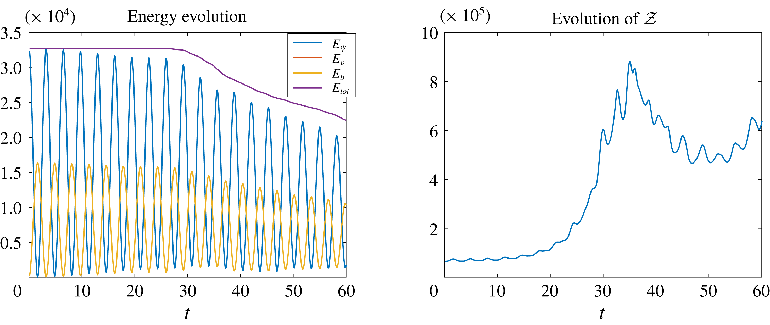
. The evolutions of the energy and rotating–stratified enstrophy are shown in figure 1 where here and below time is measured in units of
 $1/N=1$
. We observe a clear and robust enstrophy increase. At later time because of the generation of small-scale structures dissipation is not negligible, so the total energy decreases monotonously, but the rotating–stratified enstrophy increases intermittently. The snapshots of
 $\unicode[STIX]{x1D714}=\unicode[STIX]{x1D6FB}^{2}\unicode[STIX]{x1D713}$
and
 $\unicode[STIX]{x1D703}$
at
 $t=30$
and
 $60$
are shown in figure 2. Because of the wave nature of the rotating stratified system, oscillations are seen in both the energy evolutions and the snapshots.
Evolution of the energy and rotating–stratified enstrophy of the free-decay simulation.

Free-decay snapshots of
 $\unicode[STIX]{x1D714}$
and
 $\unicode[STIX]{x1D703}$
at
 $t=30$
and
 $60$
.

4 Structure function
The direction of the energy flux can be measured from the third-order structure functions based on the classical Kármán–Howarth–Monin (KHM) equation. For the most part, the correlation-function equations to be derived are not restricted to the special case
 $f=N$
, so in this section we derive the KHM equations for the general two-dimensional rotating stratified system, starting from the dimensional forced–dissipative equations
 $$\begin{eqnarray}\displaystyle & \displaystyle u_{t}+uu_{x}+wu_{z}-fv=-p_{x}+F_{u}+\unicode[STIX]{x1D708}\unicode[STIX]{x1D6FB}^{2}u, & \displaystyle\end{eqnarray}$$
 $$\begin{eqnarray}\displaystyle & \displaystyle v_{t}+uv_{x}+wv_{z}+fu=F_{v}+\unicode[STIX]{x1D708}\unicode[STIX]{x1D6FB}^{2}v, & \displaystyle\end{eqnarray}$$
 $$\begin{eqnarray}\displaystyle & \displaystyle w_{t}+uw_{x}+ww_{z}-b=-p_{z}+F_{w}+\unicode[STIX]{x1D708}\unicode[STIX]{x1D6FB}^{2}w, & \displaystyle\end{eqnarray}$$
 $$\begin{eqnarray}\displaystyle & \displaystyle b_{t}+ub_{x}+wb_{z}+N^{2}w=F_{b}+\unicode[STIX]{x1D707}\unicode[STIX]{x1D6FB}^{2}b, & \displaystyle\end{eqnarray}$$
 $$\begin{eqnarray}\displaystyle & \displaystyle u_{x}+w_{z}=0. & \displaystyle\end{eqnarray}$$
 $F$
are the external forcings, and the dissipative terms are the standard viscous and diffusive terms with viscosity
 $\unicode[STIX]{x1D708}$
and diffusivity
 $\unicode[STIX]{x1D707}$
. Different from the forced–dissipative two-dimensional turbulence, where the existence of a statistically steady state requires large-scale damping, we anticipate that in the present rotating stratified fluid system (4.1) small-scale dissipation will be sufficient, based on our heuristic downscale energy flux theory in § 3.
To derive the KHM equation we consider the fields evaluated at two positions
 $\boldsymbol{x}_{1}$
and
 $\boldsymbol{x}_{2}$
and denote them with subindices
 $_{1}$
and
 $_{2}$
, respectively (cf. Xie & Bühler (Reference Xie and Bühler2018)). This means, for example, that
 $u_{1}=u(\boldsymbol{x}_{1},t)$
and
 $u_{2}=u(\boldsymbol{x}_{2},t)$
. Then homogeneity implies that the covariance
 $$\begin{eqnarray}\displaystyle \overline{u(\boldsymbol{x}_{1},t)u(\boldsymbol{x}_{2},t)}=\overline{u_{1}u_{2}}(\boldsymbol{x},t), & & \displaystyle\end{eqnarray}$$
where the overbar denotes statistical averaging, depends only on the separation vector
 $\boldsymbol{x}=\boldsymbol{x}_{2}-\boldsymbol{x}_{1}$
. By construction, gradients of any mean field with respect to
 $\boldsymbol{x},\,\boldsymbol{x}_{1}\,\text{and}\,\boldsymbol{x}_{2}$
obey
 $$\begin{eqnarray}\displaystyle \unicode[STIX]{x1D735}=-\unicode[STIX]{x1D735}_{1}=\unicode[STIX]{x1D735}_{2}. & & \displaystyle\end{eqnarray}$$
Evaluating the governing equation (4.1) at
 $\boldsymbol{x}_{1}$
and
 $\boldsymbol{x}_{2}$
, multiplying
 $u$
,
 $v$
,
 $w$
and
 $b$
at the conjugate locations, adding and averaging (cf. Monin & Yaglom Reference Monin and Yaglom1975; Frisch Reference Frisch1995) yields
 $$\begin{eqnarray}\displaystyle & & \displaystyle {\displaystyle \frac{1}{2}}\unicode[STIX]{x2202}_{t}\overline{u_{1}u_{2}}-{\displaystyle \frac{1}{4}}\unicode[STIX]{x1D735}\boldsymbol{\cdot }\overline{\unicode[STIX]{x1D6FF}\boldsymbol{u}\unicode[STIX]{x1D6FF}u^{2}}-{\displaystyle \frac{f}{2}}\overline{u_{1}v_{2}+u_{2}v_{1}}\nonumber\\ \displaystyle & & \displaystyle \quad ={\displaystyle \frac{1}{2}}\overline{p_{1}u_{x2}-p_{2}u_{1x}}+{\displaystyle \frac{1}{2}}\overline{F_{u1}u_{2}+F_{u2}u_{1}}+\unicode[STIX]{x1D708}\unicode[STIX]{x1D6FB}^{2}\overline{u_{1}u_{2}},\end{eqnarray}$$
 $$\begin{eqnarray}\displaystyle & & \displaystyle {\displaystyle \frac{1}{2}}\unicode[STIX]{x2202}_{t}\overline{v_{1}v_{2}}-{\displaystyle \frac{1}{4}}\unicode[STIX]{x1D735}\boldsymbol{\cdot }\overline{\unicode[STIX]{x1D6FF}\boldsymbol{u}\unicode[STIX]{x1D6FF}v^{2}}+\frac{f}{2}\overline{u_{1}v_{2}+u_{2}v}={\displaystyle \frac{1}{2}}\overline{F_{v1}v_{2}+F_{v2}v}+\unicode[STIX]{x1D708}\unicode[STIX]{x1D6FB}^{2}\overline{v_{1}v_{2}},\end{eqnarray}$$
 $$\begin{eqnarray}\displaystyle & & \displaystyle {\displaystyle \frac{1}{2}}\unicode[STIX]{x2202}_{t}\overline{w_{1}w_{2}}-{\displaystyle \frac{1}{4}}\unicode[STIX]{x1D735}\boldsymbol{\cdot }\overline{\unicode[STIX]{x1D6FF}\boldsymbol{u}\unicode[STIX]{x1D6FF}w^{2}}-{\displaystyle \frac{1}{2}}\overline{w_{1}b_{2}+w_{2}b_{1}}\nonumber\\ \displaystyle & & \displaystyle \quad ={\displaystyle \frac{1}{2}}\overline{p_{1}u_{z2}-p_{2}u_{z1}}+{\displaystyle \frac{1}{2}}\overline{F_{w1}w_{2}+F_{w2}w}+\unicode[STIX]{x1D708}\unicode[STIX]{x1D6FB}^{2}\overline{w_{1}w_{2}},\end{eqnarray}$$
 $$\begin{eqnarray}\displaystyle & & \displaystyle {\displaystyle \frac{1}{2N^{2}}}\unicode[STIX]{x2202}_{t}\overline{b_{1}b_{2}}-{\displaystyle \frac{1}{4N^{2}}}\unicode[STIX]{x1D735}\boldsymbol{\cdot }\overline{\unicode[STIX]{x1D6FF}\boldsymbol{u}\unicode[STIX]{x1D6FF}b^{2}}+{\displaystyle \frac{1}{2}}\overline{w_{1}b_{2}+w_{2}b_{1}}\nonumber\\ \displaystyle & & \displaystyle \quad ={\displaystyle \frac{1}{2N^{2}}}\overline{F_{b1}b_{2}+F_{b2}b_{1}}+{\displaystyle \frac{\unicode[STIX]{x1D707}}{N^{2}}}\unicode[STIX]{x1D6FB}^{2}\overline{b_{1}b_{2}}.\end{eqnarray}$$
 $\unicode[STIX]{x1D6FF}$
means
 $\unicode[STIX]{x1D6FF}u=u_{2}-u_{1}$
, etc. Adding (4.4a
) and (4.4c
) cancels the pressure terms via incompressibility (4.1e
), and we obtain
 $$\begin{eqnarray}\displaystyle & & \displaystyle {\displaystyle \frac{1}{2}}\unicode[STIX]{x2202}_{t}\left(\overline{u_{1}u_{2}}+\overline{w_{1}w_{2}}\right)-{\displaystyle \frac{1}{4}}\unicode[STIX]{x1D735}\boldsymbol{\cdot }\overline{\unicode[STIX]{x1D6FF}\boldsymbol{u}\left(\unicode[STIX]{x1D6FF}u^{2}+\unicode[STIX]{x1D6FF}w^{2}\right)}-{\displaystyle \frac{f}{2}}\overline{u_{1}v_{2}+u_{2}v_{1}}-{\displaystyle \frac{1}{2}}\overline{w_{1}b_{2}+w_{2}b_{1}}\nonumber\\ \displaystyle & & \displaystyle \quad ={\displaystyle \frac{1}{2}}\overline{F_{u1}u_{2}+F_{u2}u_{1}}+{\displaystyle \frac{1}{2}}\overline{F_{w1}w_{2}+F_{w2}w_{1}}+\unicode[STIX]{x1D708}\unicode[STIX]{x1D6FB}^{2}\overline{u_{1}u_{2}}+\unicode[STIX]{x1D708}\unicode[STIX]{x1D6FB}^{2}\overline{w_{1}w_{2}}.\end{eqnarray}$$
Similarly, adding (4.4b ) and (4.4d ) results in
 $$\begin{eqnarray}\displaystyle & & \displaystyle {\displaystyle \frac{1}{2}}\unicode[STIX]{x2202}_{t}\left(\overline{v_{1}v_{2}}+{\displaystyle \frac{\overline{b_{1}b_{2}}}{N^{2}}}\right)-{\displaystyle \frac{1}{4}}\unicode[STIX]{x1D735}\boldsymbol{\cdot }\overline{\unicode[STIX]{x1D6FF}\boldsymbol{u}\left(\unicode[STIX]{x1D6FF}v^{2}+{\displaystyle \frac{\unicode[STIX]{x1D6FF}b^{2}}{N^{2}}}\right)}+{\displaystyle \frac{f}{2}}\overline{u_{1}v_{2}+u_{2}v_{1}}+{\displaystyle \frac{1}{2}}\overline{w_{1}b_{2}+w_{2}b_{1}}\nonumber\\ \displaystyle & & \displaystyle \quad ={\displaystyle \frac{1}{2}}\overline{F_{v1}v_{2}+F_{v2}v_{1}}+{\displaystyle \frac{1}{2N^{2}}}\overline{F_{b1}b_{2}+F_{b2}b_{1}}+\unicode[STIX]{x1D708}\unicode[STIX]{x1D6FB}^{2}\overline{v_{1}v_{2}}+{\displaystyle \frac{\unicode[STIX]{x1D707}}{N^{2}}}\unicode[STIX]{x1D6FB}^{2}\overline{b_{1}b_{2}}.\end{eqnarray}$$
We name these equations the KHM equations for the kinetic and effective potential energy, respectively, where the effective potential energy also contains the scalar
 $v$
. Considering the opposite signs of the conversion terms in (4.5) and (4.6), by adding them we cancel the conversion term and obtain the KHM equation for the total energy,
 $$\begin{eqnarray}\displaystyle & & \displaystyle {\displaystyle \frac{1}{2}}\unicode[STIX]{x2202}_{t}\left(\overline{u_{1}u_{2}}+\overline{w_{1}w_{2}}+\overline{v_{1}v_{2}}+{\displaystyle \frac{\overline{b_{1}b_{2}}}{N^{2}}}\right)\nonumber\\ \displaystyle & & \displaystyle \qquad -{\displaystyle \frac{1}{4}}\unicode[STIX]{x1D735}\boldsymbol{\cdot }\overline{\unicode[STIX]{x1D6FF}\boldsymbol{u}\left(\unicode[STIX]{x1D6FF}u^{2}+\unicode[STIX]{x1D6FF}w^{2}+\unicode[STIX]{x1D6FF}v^{2}+{\displaystyle \frac{\unicode[STIX]{x1D6FF}b^{2}}{N^{2}}}\right)}=P(\boldsymbol{x})+D(\boldsymbol{x}),\end{eqnarray}$$
where
 $$\begin{eqnarray}\displaystyle \displaystyle P(\boldsymbol{x}) & = & \displaystyle {\displaystyle \frac{1}{2}}\overline{F_{u1}u_{2}+F_{u2}u_{1}}+{\displaystyle \frac{1}{2}}\overline{F_{w1}w_{2}+F_{w2}w_{1}}\nonumber\\ \displaystyle & & \displaystyle +{\displaystyle \frac{1}{2}}\overline{F_{v1}v_{2}+F_{v2}v_{1}}+{\displaystyle \frac{1}{2N^{2}}}\overline{F_{b1}b_{2}+F_{b2}b_{1}}\end{eqnarray}$$
 $$\begin{eqnarray}\displaystyle & & \displaystyle \displaystyle \text{and}\quad D(\boldsymbol{x})=\unicode[STIX]{x1D708}\unicode[STIX]{x1D6FB}^{2}\overline{u_{1}u_{2}}+\unicode[STIX]{x1D708}\unicode[STIX]{x1D6FB}^{2}\overline{w_{1}w_{2}}+\unicode[STIX]{x1D708}\unicode[STIX]{x1D6FB}^{2}\overline{v_{1}v_{2}}+{\displaystyle \frac{\unicode[STIX]{x1D707}}{N^{2}}}\unicode[STIX]{x1D6FB}^{2}\overline{b_{1}b_{2}},\end{eqnarray}$$
 $$\begin{eqnarray}\displaystyle \unicode[STIX]{x1D716}=P(0) & & \displaystyle\end{eqnarray}$$
is the mean energy input rate per unit time and mass.
4.1 Special case
$f=N$
and
$\unicode[STIX]{x1D707}=\unicode[STIX]{x1D708}$


We now restrict to
 $f=N$
and
 $\unicode[STIX]{x1D708}=\unicode[STIX]{x1D707}$
, make time non-dimensional with
 $1/N$
and use
 $\unicode[STIX]{x1D703}=b/N$
, as before. This yields
 $$\begin{eqnarray}\displaystyle & & \displaystyle {\displaystyle \frac{1}{2}}\unicode[STIX]{x2202}_{t}\left(\overline{u_{1}u_{2}}+\overline{w_{1}w_{2}}\right)-{\displaystyle \frac{1}{4}}\unicode[STIX]{x1D735}\boldsymbol{\cdot }\overline{\unicode[STIX]{x1D6FF}\boldsymbol{u}\left(\unicode[STIX]{x1D6FF}u^{2}+\unicode[STIX]{x1D6FF}w^{2}\right)}-\frac{1}{2}\overline{u_{1}v_{2}+u_{2}v_{1}}-{\displaystyle \frac{1}{2}}\overline{w_{1}\unicode[STIX]{x1D703}_{2}+w_{2}\unicode[STIX]{x1D703}_{1}}\nonumber\\ \displaystyle & & \displaystyle \quad ={\displaystyle \frac{1}{2}}\overline{F_{u1}u_{2}+F_{u2}u_{1}}+{\displaystyle \frac{1}{2}}\overline{F_{w1}w_{2}+F_{w2}w_{1}}+\unicode[STIX]{x1D708}\unicode[STIX]{x1D6FB}^{2}\overline{u_{1}u_{2}}+\unicode[STIX]{x1D708}\unicode[STIX]{x1D6FB}^{2}\overline{w_{1}w_{2}}\end{eqnarray}$$
and
 $$\begin{eqnarray}\displaystyle & & \displaystyle {\displaystyle \frac{1}{2}}\unicode[STIX]{x2202}_{t}\left(\overline{v_{1}v_{2}}+\overline{\unicode[STIX]{x1D703}_{1}\unicode[STIX]{x1D703}_{2}}\right)-{\displaystyle \frac{1}{4}}\unicode[STIX]{x1D735}\boldsymbol{\cdot }\overline{\unicode[STIX]{x1D6FF}\boldsymbol{u}\left(\unicode[STIX]{x1D6FF}v^{2}+\unicode[STIX]{x1D6FF}\unicode[STIX]{x1D703}^{2}\right)}+\frac{1}{2}\overline{u_{1}v_{2}+u_{2}v_{1}}+{\displaystyle \frac{1}{2}}\overline{w_{1}\unicode[STIX]{x1D703}_{2}+w_{2}\unicode[STIX]{x1D703}_{1}}\nonumber\\ \displaystyle & & \displaystyle \quad ={\displaystyle \frac{1}{2}}\overline{F_{v1}v_{2}+F_{v2}v_{1}}+{\displaystyle \frac{1}{2}}\overline{F_{\unicode[STIX]{x1D703}1}\unicode[STIX]{x1D703}_{2}+F_{\unicode[STIX]{x1D703}2}\unicode[STIX]{x1D703}_{1}}+\unicode[STIX]{x1D708}\unicode[STIX]{x1D6FB}^{2}\overline{v_{1}v_{2}}+\unicode[STIX]{x1D708}\unicode[STIX]{x1D6FB}^{2}\overline{\unicode[STIX]{x1D703}_{1}\unicode[STIX]{x1D703}_{2}}.\end{eqnarray}$$
Adding (4.10) and (4.11) we obtain the KHM equation corresponding to (4.5),
 $$\begin{eqnarray}\displaystyle & & \displaystyle {\displaystyle \frac{1}{2}}\unicode[STIX]{x2202}_{t}\left(\overline{u_{1}u_{2}}+\overline{w_{1}w_{2}}+\overline{v_{1}v_{2}}+\overline{\unicode[STIX]{x1D703}_{1}\unicode[STIX]{x1D703}_{2}}\right)\nonumber\\ \displaystyle & & \displaystyle \qquad -{\displaystyle \frac{1}{4}}\unicode[STIX]{x1D735}\boldsymbol{\cdot }\overline{\unicode[STIX]{x1D6FF}\boldsymbol{u}\left(\unicode[STIX]{x1D6FF}u^{2}+\unicode[STIX]{x1D6FF}w^{2}+\unicode[STIX]{x1D6FF}v^{2}+\unicode[STIX]{x1D6FF}\unicode[STIX]{x1D703}^{2}\right)}=P(\boldsymbol{x})+D(\boldsymbol{x}),\end{eqnarray}$$
where
 $$\begin{eqnarray}\displaystyle \displaystyle P(\boldsymbol{x}) & = & \displaystyle {\displaystyle \frac{1}{2}}\overline{F_{u1}u_{2}+F_{u2}u_{1}}+{\displaystyle \frac{1}{2}}\overline{F_{w1}w_{2}+F_{w2}w_{1}}\nonumber\\ \displaystyle & & \displaystyle +{\displaystyle \frac{1}{2}}\overline{F_{v1}v_{2}+F_{v2}v_{1}}+{\displaystyle \frac{1}{2}}\overline{F_{\unicode[STIX]{x1D703}1}\unicode[STIX]{x1D703}_{2}+F_{\unicode[STIX]{x1D703}2}\unicode[STIX]{x1D703}_{1}},\end{eqnarray}$$
 $$\begin{eqnarray}D(\boldsymbol{x})=\unicode[STIX]{x1D708}\unicode[STIX]{x1D6FB}^{2}\left(\overline{u_{1}u_{2}}+\overline{w_{1}w_{2}}+\overline{v_{1}v_{2}}+\overline{\unicode[STIX]{x1D703}_{1}\unicode[STIX]{x1D703}_{2}}\right)\!.\end{eqnarray}$$
4.2 Structure functions for isotropic turbulence
We now assume that the forcing and dissipation functions are isotropic, i.e. both
 $P$
and
 $D$
depend only on
 $r=|\boldsymbol{x}|$
. In this isotropic set-up the conversion term,
 $$\begin{eqnarray}\displaystyle {\displaystyle \frac{1}{2}}\overline{u_{1}v_{2}+u_{2}v_{1}}+{\displaystyle \frac{1}{2}}\overline{w_{1}\unicode[STIX]{x1D703}_{2}+w_{2}\unicode[STIX]{x1D703}_{1}}, & & \displaystyle\end{eqnarray}$$
is also invariant under the coordinates rotation (2.11), (2.13) and (2.12), so not only the third-order structure functions in the KHM equation (4.12) but also those in (4.10) and (4.11) are isotropic. This means we can express them as
 $$\begin{eqnarray}\displaystyle & \displaystyle \overline{\unicode[STIX]{x1D6FF}\boldsymbol{u}\left(\unicode[STIX]{x1D6FF}u^{2}+\unicode[STIX]{x1D6FF}w^{2}\right)}=\boldsymbol{V}_{K}=V_{K}(r){\displaystyle \frac{\boldsymbol{x}}{r}}, & \displaystyle\end{eqnarray}$$
 $$\begin{eqnarray}\displaystyle & \displaystyle \overline{\unicode[STIX]{x1D6FF}\boldsymbol{u}\left(\unicode[STIX]{x1D6FF}v^{2}+\unicode[STIX]{x1D6FF}\unicode[STIX]{x1D703}^{2}\right)}=\boldsymbol{V}_{P}=V_{P}(r){\displaystyle \frac{\boldsymbol{x}}{r}}, & \displaystyle\end{eqnarray}$$
 $$\begin{eqnarray}\displaystyle & \displaystyle \overline{\unicode[STIX]{x1D6FF}\boldsymbol{u}\left(\unicode[STIX]{x1D6FF}u^{2}+\unicode[STIX]{x1D6FF}w^{2}+\unicode[STIX]{x1D6FF}v^{2}+\unicode[STIX]{x1D6FF}\unicode[STIX]{x1D703}^{2}\right)}=\mathbf{V}=V(r){\displaystyle \frac{\boldsymbol{x}}{r}}, & \displaystyle\end{eqnarray}$$
 $V=V_{K}+V_{P}$
. All three structure functions are interesting, but at present we only have a systematic strategy for computing their sum, the total
 $V(r)$
.
4.3 Exact non-dissipative results
By assuming a downscale energy cascade a statistically steady state, i.e.
 $\unicode[STIX]{x2202}_{t}=0$
, can be reached with small-scale dissipation only, as in the familiar case of three-dimensional turbulence. Hence we obtain
 $$\begin{eqnarray}\displaystyle -{\displaystyle \frac{1}{4}}\unicode[STIX]{x1D735}\boldsymbol{\cdot }\boldsymbol{V}=P(r)+\unicode[STIX]{x1D708}\unicode[STIX]{x1D6FB}^{2}\left(\overline{u_{1}u_{2}}+\overline{w_{1}w_{2}}+\overline{v_{1}v_{2}}+\overline{\unicode[STIX]{x1D703}_{1}\unicode[STIX]{x1D703}_{2}}\right)\!, & & \displaystyle\end{eqnarray}$$
which, using
 $\unicode[STIX]{x1D735}\,\overline{\unicode[STIX]{x1D6FF}u^{2}}=-2\unicode[STIX]{x1D735}\,\overline{u_{1}u_{2}}$
and
 $V(0)=0$
, can be integrated to obtain
 $$\begin{eqnarray}\displaystyle V(r)=-{\displaystyle \frac{4}{r}}\int _{0}^{r}P(s)s\,\text{d}s+2\unicode[STIX]{x1D708}{\displaystyle \frac{\text{d}}{\text{d}r}}\left(\overline{\unicode[STIX]{x1D6FF}u^{2}}+\overline{\unicode[STIX]{x1D6FF}v^{2}}+\overline{\unicode[STIX]{x1D6FF}w^{2}}+\overline{\unicode[STIX]{x1D6FF}\unicode[STIX]{x1D703}^{2}}\right)\!. & & \displaystyle\end{eqnarray}$$
This equation is the two-dimensional counterpart of (2.17) in Xie & Bühler (Reference Xie and Bühler2018). In the inertial range we ignore the dissipation term and obtain
 $$\begin{eqnarray}\displaystyle V(r)=-{\displaystyle \frac{4}{r}}\int _{0}^{r}P(s)s\,\text{d}s. & & \displaystyle\end{eqnarray}$$
Even though the system (4.1) is two-dimensional, because of downscale energy transfer its third-order structure function theory is more similar to that of three-dimensional turbulence (Kolmogorov Reference Kolmogorov1941) than that of two-dimensional turbulence (Bernard Reference Bernard1999; Lindborg Reference Lindborg1999; Yakhot Reference Yakhot1999; Xie & Bühler Reference Xie and Bühler2018).
For a temporal white-noise external force
 $P(r)$
is proportional to the spatial structure functions of the external force (Bernard Reference Bernard1999), and if the forcing in spectral space is
 $\unicode[STIX]{x1D6FF}$
-centred at some forcing wavenumber
 $k_{f}$
, say, then
 $$\begin{eqnarray}\displaystyle P(r)=\unicode[STIX]{x1D716}J_{0}(k_{f}r), & & \displaystyle\end{eqnarray}$$
with
 $J_{0}$
the zeroth-order Bessel function (cf. Xie & Bühler (Reference Xie and Bühler2018)). Substituting in (4.18) we obtain
 $$\begin{eqnarray}\displaystyle V(r)=-4{\displaystyle \frac{\unicode[STIX]{x1D716}}{k_{f}}}J_{1}(k_{f}r). & & \displaystyle\end{eqnarray}$$
When
 $k_{f}r\ll 1$
, we asymptotically obtain
 $V\sim -2\unicode[STIX]{x1D716}r$
. Unsurprisingly, this asymptotic result is identical to that of Grossmann & Mertens (Reference Grossmann and Mertens1992), which is obtained by assuming a downscale energy flux in standard two-dimensional turbulence. It remains to be checked that energy indeed flows downscale, as suggested by our heuristic argument in § 3. To establish this we turn to direct numerical simulations.
5 Numerical simulations
In this section we present the numerical results of the forced–dissipative rotating stratified fluid system (4.1) in a doubly periodic domain of size
 $2\unicode[STIX]{x03C0}\times 2\unicode[STIX]{x03C0}$
with external forcing that is a temporal white noise with energy input rate
 $\unicode[STIX]{x1D716}$
and a spatial structure given by a delta function at some
 $k_{f}$
in wavenumber space, so (4.20) applies. To maintain a uniform PV
 $q=f$
, the external forcing is restricted to the
 $xz$
-momentum equations, i.e.
 $F_{v}=F_{\unicode[STIX]{x1D703}}=0$
. Thus we only force the wave component whilst the potential vorticity
 $q$
and the associated balanced components are not forced. However, the dissipation terms create a small amount of PV spontaneously, so the PV does not remain exactly zero. We checked numerically that this small amount of PV is not relevant by performing test simulations where the PV is set to zero at each time step.
Because of the incompressibility,
 $F_{u}$
and
 $F_{w}$
are calculated through a scalar field
 $\unicode[STIX]{x1D6F9}$
such that
 $(F_{u},\,F_{w})=\unicode[STIX]{x1D735}^{\bot }\unicode[STIX]{x1D6F9}$
. At each time step, the forcing is defined in Fourier space by
 $$\begin{eqnarray}\displaystyle \hat{\unicode[STIX]{x1D6F9}}=-C{\displaystyle \frac{\unicode[STIX]{x1D716}^{1/2}}{k_{f}}}\text{e}^{-(K-k_{f})^{2}/2\unicode[STIX]{x0394}K}G(k,l), & & \displaystyle\end{eqnarray}$$
where
 $\hat{\cdot }$
denotes the Fourier transform,
 $C$
is a normalization constant,
 $K=\sqrt{k^{2}+m^{2}}$
,
 $\unicode[STIX]{x0394}K$
measures the concentration of forcing in the spectral space and
 $G$
is a unit variance Gaussian random variable, which is designed to ensure a real
 $\unicode[STIX]{x1D713}$
. In our simulations
 $\unicode[STIX]{x0394}K=1$
and
 $C$
is a chosen number which makes the total energy input rate equals
 $\unicode[STIX]{x1D716}$
.
From dimensional analysis, we define the usual Ozmidov scale
 $$\begin{eqnarray}\displaystyle l_{O}=1/k_{O}=\unicode[STIX]{x1D716}^{1/2}/N^{3/2}=\unicode[STIX]{x1D716}^{1/2}/f^{3/2} & & \displaystyle\end{eqnarray}$$
as the scale at which the nonlinear time scale matches the linear, wave time scale. Basically, the size of
 $l_{O}$
measures the strength of the forcing, i.e. the stronger the forcing the larger
 $l_{O}$
will be. The overall dynamics of the turbulent system is controlled by the relative size of
 $l_{f}$
and
 $l_{O}$
. We explore the range of possibilities by showing three simulations with
 $l_{O}\gg l_{f}$
,
 $l_{O}\sim l_{f}$
and
 $l_{O}\ll l_{f}$
, respectively. We name these three regimes the strong forcing regime, intermediate forcing regime and weak forcing regime. It will be seen that in each case the downscale total energy flux predicted in § 3 is verified and the corresponding structure functions agree with the theory.
We apply hyperviscosity operators
 $\unicode[STIX]{x1D708}_{h}\unicode[STIX]{x1D6FB}^{6}$
to all fields, which by dimensional analysis introduces the dissipation scale
 $l_{\unicode[STIX]{x1D708}}=1/k_{\unicode[STIX]{x1D708}}=(\unicode[STIX]{x1D708}_{h}^{3}/\unicode[STIX]{x1D716})^{1/16}$
. With adjusted coefficients
 $\unicode[STIX]{x1D708}_{h}=10^{-13},\,5\times 10^{-13}$
and
 $10^{-13}$
for the three simulations, the dissipation scales are
 $l_{\unicode[STIX]{x1D708}}\approx 0.005,\,0.0067$
and
 $0.0067$
, which correspond to
 $k_{\unicode[STIX]{x1D708}}\approx 200,\,150$
and
 $150$
, respectively. We chose a smaller dissipation scale for the first simulation because we want to observe a clear downscale energy flux when the forcing is strong. The initial conditions are zero in each run. The parameters used in the three simulations in the following subsections are shown in table 1. Notably,
 $l_{O}$
is smaller than the domain size in all cases.
Parameters used in the numerical simulations.

5.1 Strong forcing regime (
$l_{O}\gg l_{f}$
)

In this section we show the result of a simulation with
 $l_{O}\gg l_{f}$
by choosing
 $k_{f}=64$
and
 $\unicode[STIX]{x1D716}=0.01$
in (5.1), therefore the Ozmidov wavenumber
 $k_{O}\approx 10$
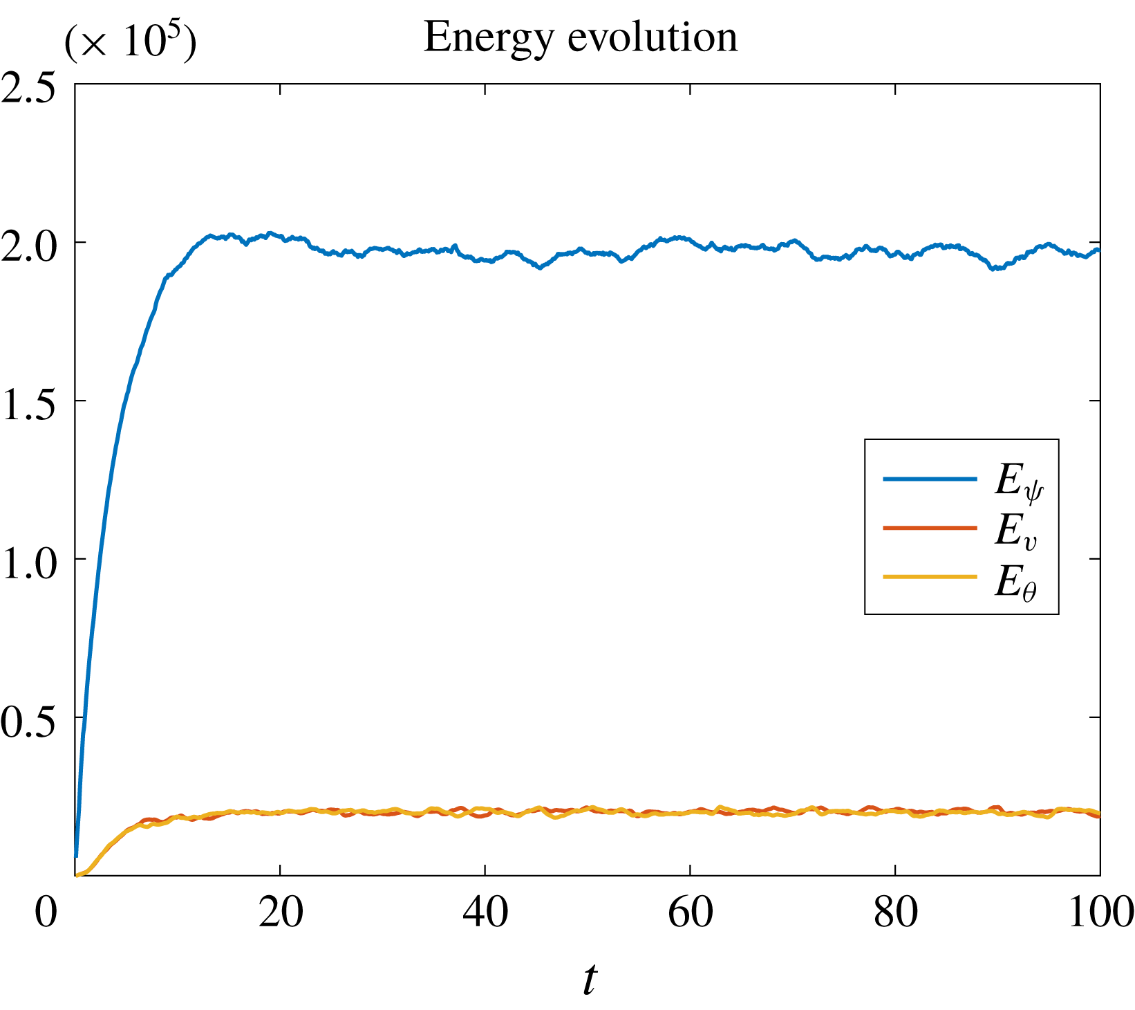
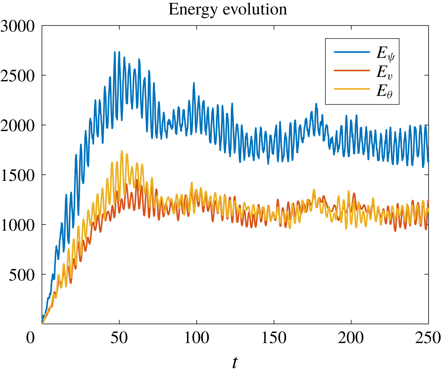
and the Ozmidov scale is much larger than the forcing scale. We show the energy evolution in figure 3. At the final state the kinetic energy
 $E_{\unicode[STIX]{x1D713}}=\int (u^{2}+w^{2})\,\text{d}\boldsymbol{x}/2$
, the
 $v$
-‘potential energy’
 $E_{v}=\int v^{2}\,\text{d}\boldsymbol{x}/2$
and the buoyancy potential energy
 $E_{\unicode[STIX]{x1D703}}=\int \unicode[STIX]{x1D703}^{2}\,\text{d}\boldsymbol{x}/2$
are all statistically steady. The steadiness combined with the ergodicity assumption enable us to replace ensemble averaging by time averaging, and all statistical quantities are obtained by time averaging over the interval
 $t\in [40,\,100]$
. It is clear from figure 3 that the kinetic energy is much larger than the potential energy, but nevertheless the potential energy turns out to be crucial for the overall energy dynamics. In figure 4 we show snapshots of
 $u$
,
 $w$
,
 $M=x+v$
and
 $S=z+\unicode[STIX]{x1D703}$
at time
 $t=100$
. The
 $u$
and
 $w$
figures show that they separately have patterns with directionality, but we will show later that the combinations of them in the third-order structure functions become isotropic. We also observe the similarity of the patterns and the matching magnitudes between
 $v$
and
 $\unicode[STIX]{x1D703}$
. These images show very strong deformations and curdling of the material lines of constant
 $M$
or
 $S$
at the forcing scale
 $l_{f}$
, where the excess of the kinetic energy over the potential energy is somewhat akin to a pendulum going over the top. However, at scales
 $l_{O}$
or above the restoring effect of the waves becomes important and changes the dynamics.
Energy evolution of
 $u$
- and
 $w$
-kinetic energy
 $E_{\unicode[STIX]{x1D713}}$
,
 $v$
-potential energy
 $E_{v}$
and potential energy
 $E_{\unicode[STIX]{x1D703}}$
for the strong forcing regime simulation.

Snapshots of
 $u$
,
 $w$
,
 $M=x+v$
and
 $S=z+\unicode[STIX]{x1D703}$
at time
 $t=100$
for the strong forcing simulation.

5.1.1 Spectral energy-flux diagnostics
The azimuthally integrated kinetic and effective potential energy spectral equations are
 $$\begin{eqnarray}\displaystyle & \displaystyle {\displaystyle \frac{\text{d}}{\text{d}t}}\int _{0}^{2\unicode[STIX]{x03C0}}{\displaystyle \frac{1}{2}}\{|\hat{u} |^{2}+|{\hat{w}}|^{2}\}K\,\text{d}\unicode[STIX]{x1D6FC}+{\displaystyle \frac{\text{d}}{\text{d}K}}F_{K}+C=\text{forcing}\,+\text{dissipation}, & \displaystyle\end{eqnarray}$$
 $$\begin{eqnarray}\displaystyle & \displaystyle {\displaystyle \frac{\text{d}}{\text{d}t}}\int _{0}^{2\unicode[STIX]{x03C0}}{\displaystyle \frac{1}{2}}\{|\hat{v}|^{2}+|\hat{\unicode[STIX]{x1D703}}|^{2}\}K\,\text{d}\unicode[STIX]{x1D6FC}+{\displaystyle \frac{\text{d}}{\text{d}K}}F_{P}-C=\text{dissipation}, & \displaystyle\end{eqnarray}$$
 $$\begin{eqnarray}\displaystyle & \displaystyle F_{K}=\int _{0}^{K}\int _{0}^{2\unicode[STIX]{x03C0}}{\displaystyle \frac{1}{2}}\left(\hat{u} ^{\ast }\widehat{\boldsymbol{u}\boldsymbol{\cdot }\unicode[STIX]{x1D735}u}+{\hat{w}}^{\ast }\widehat{\boldsymbol{u}\boldsymbol{\cdot }\unicode[STIX]{x1D735}w}+\text{c.c.}\right)\unicode[STIX]{x1D705}\,\text{d}\unicode[STIX]{x1D705}\,\text{d}\unicode[STIX]{x1D6FC}, & \displaystyle\end{eqnarray}$$
 $$\begin{eqnarray}\displaystyle F_{P}=\int _{0}^{K}\int _{0}^{2\unicode[STIX]{x03C0}}{\displaystyle \frac{1}{2}}\left(\hat{v}^{\ast }\widehat{\boldsymbol{u}\boldsymbol{\cdot }\unicode[STIX]{x1D735}v}+\hat{\unicode[STIX]{x1D703}}^{\ast }\widehat{\boldsymbol{u}\boldsymbol{\cdot }\unicode[STIX]{x1D735}\unicode[STIX]{x1D703}}+\text{c.c.}\right)\unicode[STIX]{x1D705}\,\text{d}\unicode[STIX]{x1D705}\,\text{d}\unicode[STIX]{x1D6FC}\end{eqnarray}$$
are the kinetic and effective potential energy fluxes, respectively,
 $$\begin{eqnarray}\displaystyle C=-\int _{0}^{2\unicode[STIX]{x03C0}}{\displaystyle \frac{1}{2}}\left(\hat{u} ^{\ast }\hat{v}+{\hat{w}}^{\ast }\hat{\unicode[STIX]{x1D703}}+\text{c.c.}\right)K\,\text{d}\unicode[STIX]{x1D6FC} & & \displaystyle\end{eqnarray}$$
is the conversion term,
 $K=\sqrt{k^{2}+m^{2}}$
,
 $\unicode[STIX]{x1D6FC}=\arctan (m/k)$
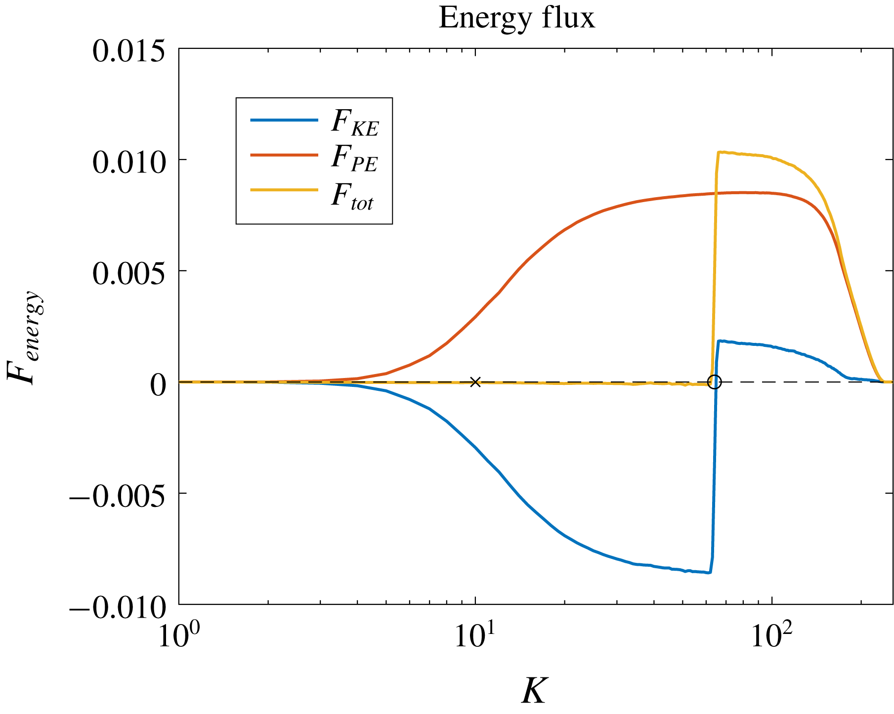
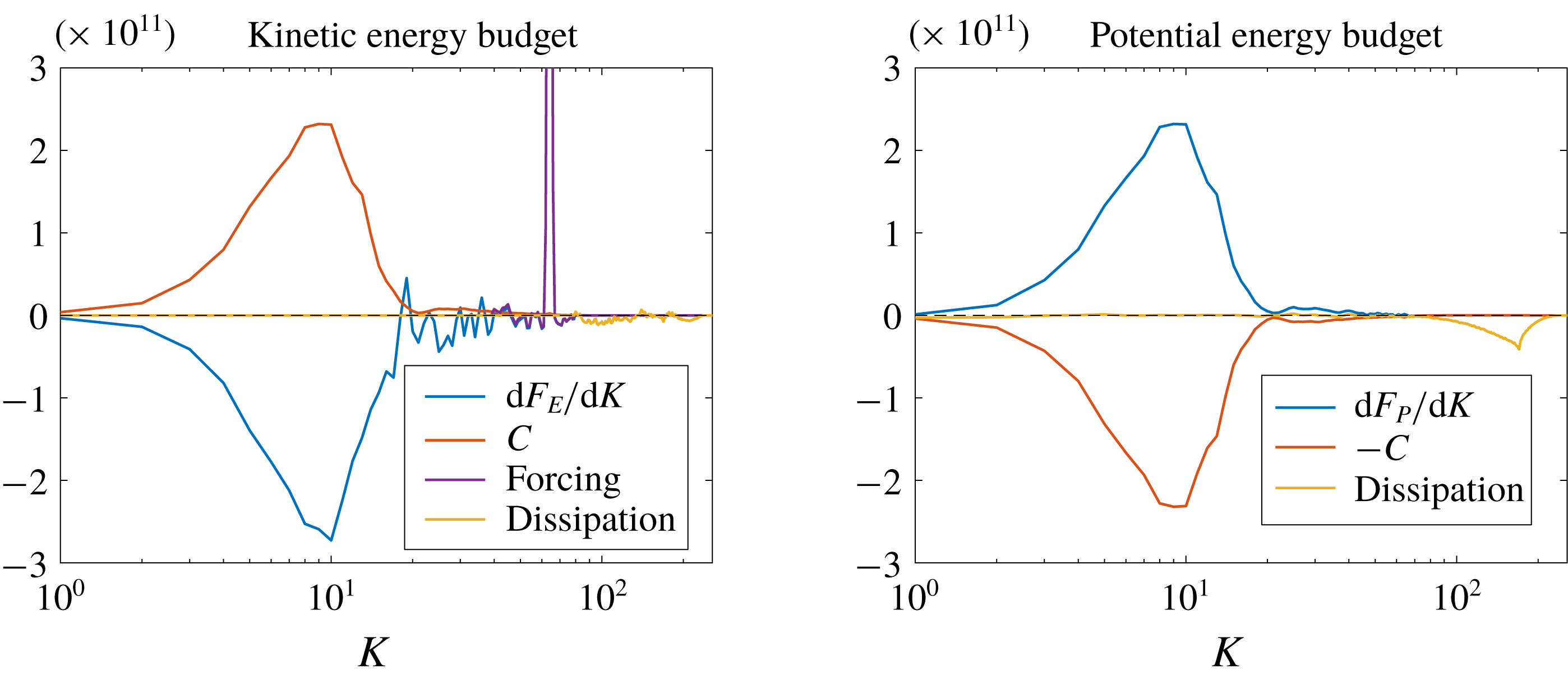
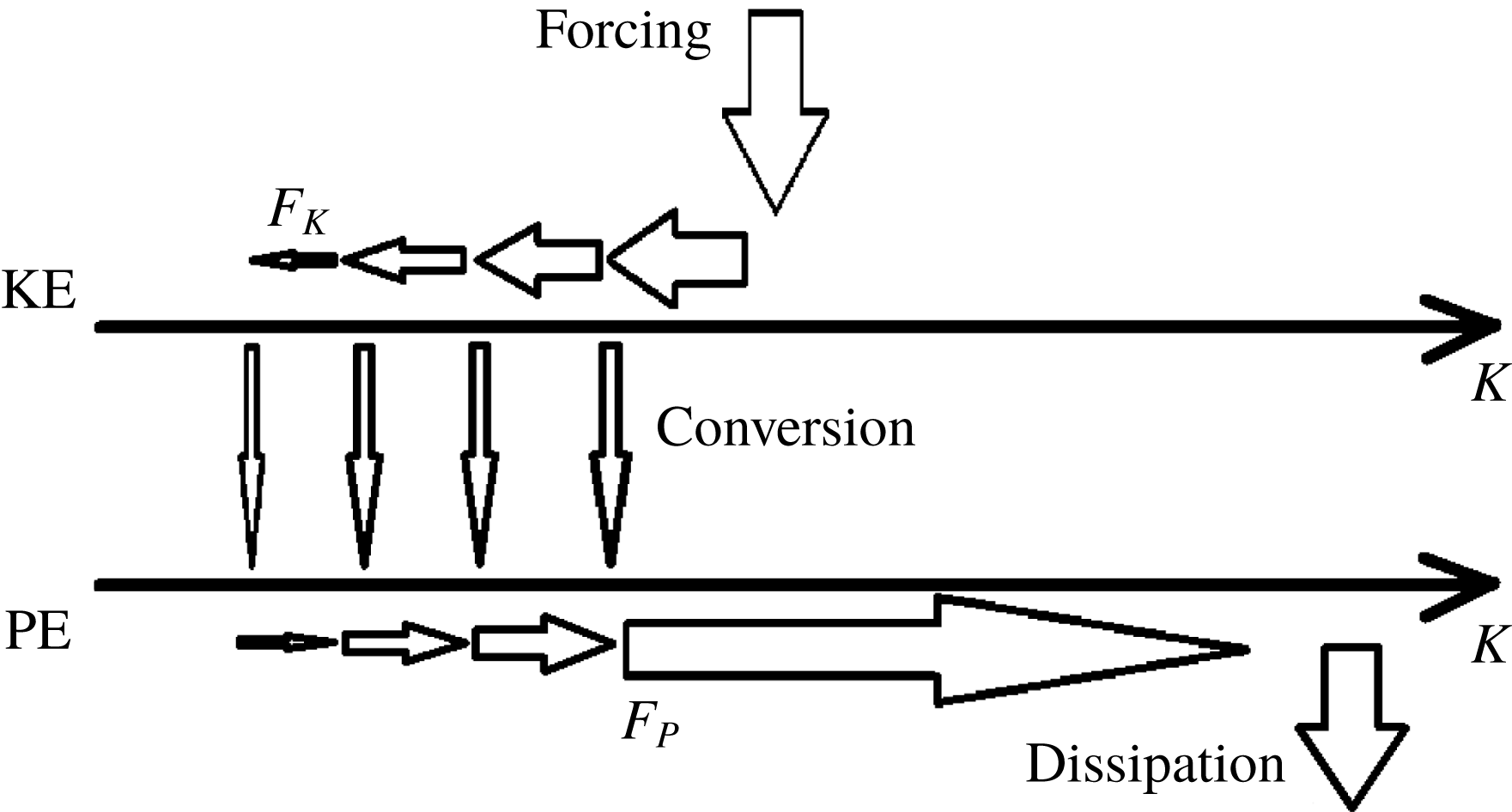
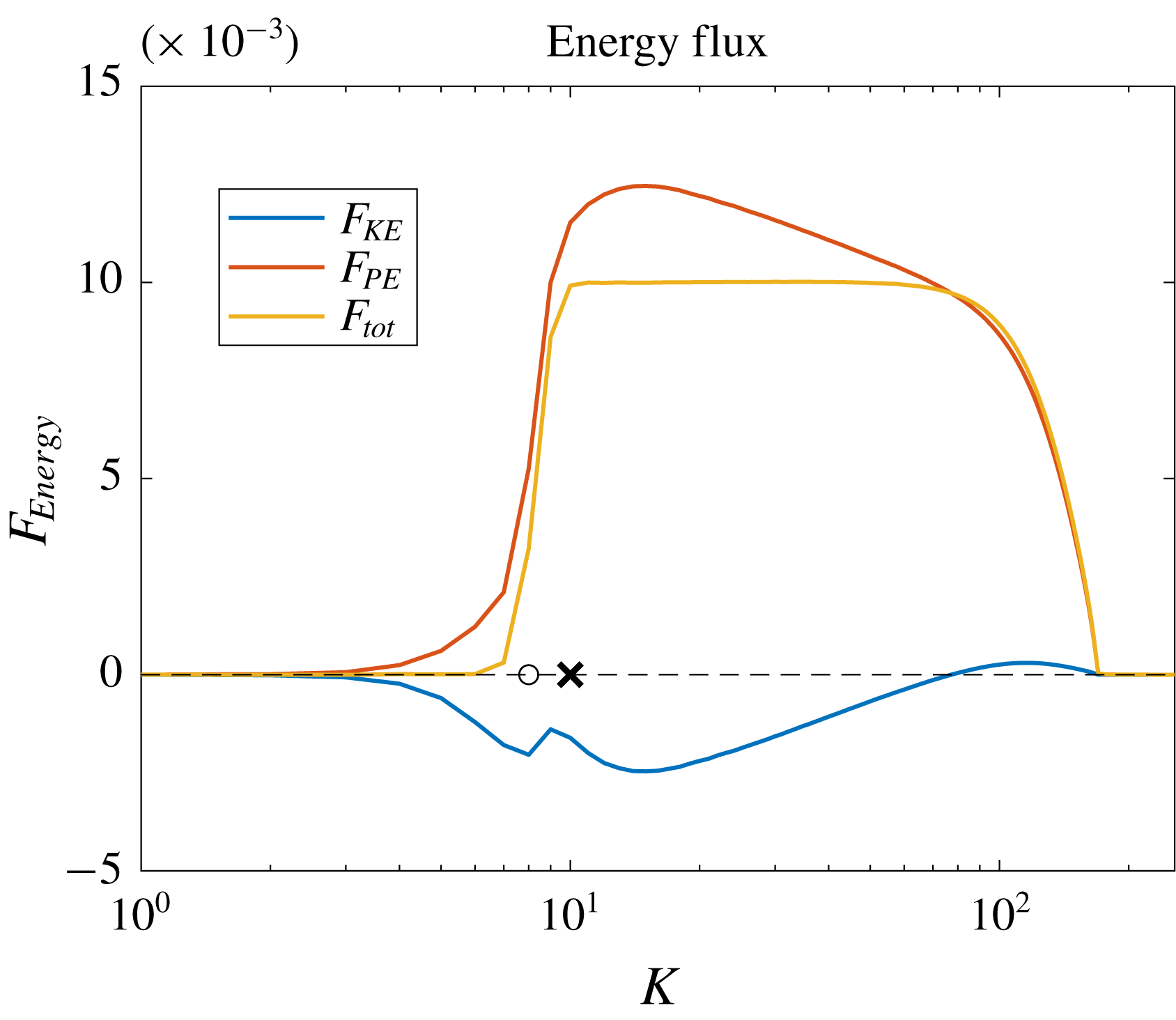
and c.c. denotes the complex conjugate. We show the energy fluxes in figure 5 and the story is as follows. The energy is injected as kinetic energy at the forcing scale, and then it is first transferred to larger scale as indicated by the negative value of the blue curve in the regime
 $K<k_{f}$
. This upscale energy transfer is expected since the buoyancy terms are weak compared with the kinetic terms when the considered wavenumber is larger than the Ozmidov wavenumber, so in this wavenumber regime, the dynamics is expected to be dominated by the inverse kinetic energy cascade of standard two-dimensional turbulence. The inverse kinetic energy flux stops at the Ozmidov wavenumber
 $k_{O}\approx 10$
, where the kinetic energy is converted into the effective potential energy of
 $v$
and
 $\unicode[STIX]{x1D703}$
. Thereafter, the effective potential energy moves downscale and is finally dissipated around the dissipation scale. Arguably, the downscale effective potential energy transfer at large wavenumbers could be expected because when
 $k>k_{O}$
the buoyancy scalars behave like passive scalars, which naturally follow downscale cascade (cf. Warhaft Reference Warhaft2000). This process is illustrated by the positive red curve.
Kinetic (
 $F_{K}$
), effective potential (
 $F_{P}$
) and total (
 $F_{tot}=F_{K}+F_{P}$
) energy fluxes for the strong forcing regime simulation. The dashed line is the
 $0$
-line which is plotted for a reference. The circle and cross mark the forcing and Ozmidov wavenumbers, respectively.

Energy budget (5.4) for the strong forcing regime simulation. The dashed lines are the residues ‘
 $\text{forcing}+\text{dissipation}-\text{d}F_{K}-C$
’ and ‘
 $\text{dissipation}-\text{d}F_{P}+C$
’ in the two panels, respectively.

Illustration of the flux-loop energy transfer processes. The upper level represents kinetic energy and the lower level represents effective potential energy;
 $F_{K}$
and
 $F_{P}$
denote the kinetic and effective potential energy transfer flux. Wavenumber increases to the right. Conversion occurs around the Ozmidov wavenumber.

In summary, the effective potential energy flux and the kinetic energy flux oppose each in other in spectral space, but the total energy transfer (yellow curve) is purely downscale due to the remarkable cancellation between the
 $F_{K}$
and
 $F_{P}$
in the regime of
 $K<k_{f}$
, justifying that we did not need a large-scale damping to ensure the system (4.1) reaches a statistically steady state. Thus, figure 5 provides direct evidence for the downscale total energy transfer, which is consistent with our heuristic argument in § 3. Combining the saturated kinetic and potential energy ratio (cf. figure 3), it is remarkable to observe that only a relatively small amount of potential energy is required to produce a net positive total energy transfer to small scales. The detailed kinetic and effective potential energy budgets (5.4) are shown in figure 6 and the illustrative figure 7 gives a cartoon of the energy-flux loop in the system. The above picture is clearest when discussed in terms of kinetic energy and effective potential energy, as the latter includes both
 $v^{2}$
and
 $b^{2}$
and those fields both follow a downscale cascade in our two-dimensional system. If instead the standard potential energy definition were used, then
 $v^{2}$
would count in the kinetic energy budget, which therefore contains a mixture of terms that move upscale as well as downscale. We checked that this would not change the qualitative picture in figure 5.
5.1.2 Isotropic structure function diagnostics
We show
 $\unicode[STIX]{x1D735}\boldsymbol{\cdot }\boldsymbol{V}_{K}$
and
 $\unicode[STIX]{x1D735}\boldsymbol{\cdot }\boldsymbol{V}_{P}$
in figure 8 to validate the isotropy assumption.
Two-dimensional
 $\unicode[STIX]{x1D735}\boldsymbol{\cdot }\boldsymbol{V}_{K}$
and
 $\unicode[STIX]{x1D735}\boldsymbol{\cdot }\boldsymbol{V}_{P}$
averaged over
 $t\in [40,\,100]$
for the strong forcing regime simulation.

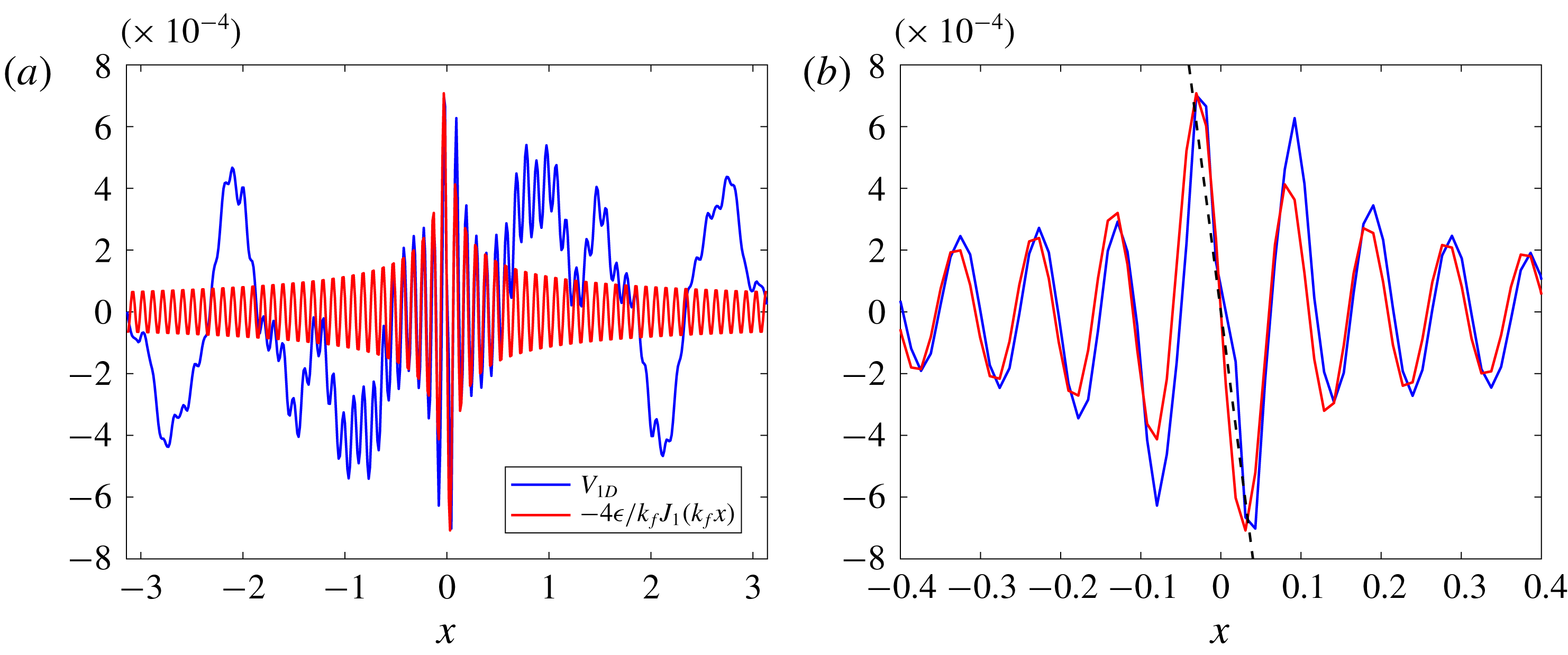
In figure 9 we show the one-dimensional ‘measurement’ along the
 $x$
-axis of
 $$\begin{eqnarray}\displaystyle V_{1D}(x)=\overline{\unicode[STIX]{x1D6FF}u(x)\left(\unicode[STIX]{x1D6FF}u(x)^{2}+\unicode[STIX]{x1D6FF}w(x)^{2}+\unicode[STIX]{x1D6FF}v(x)^{2}+\unicode[STIX]{x1D6FF}\unicode[STIX]{x1D703}(x)^{2}\right)} & & \displaystyle\end{eqnarray}$$
and compare it with the theoretical result (4.20). Even though the measurement and the theoretical results have a big discrepancy at large
 $x$
, where the convergence of the statistical quantities would require a much longer integration time, the inset shows very good matching in the region of moderate
 $x$
. Indeed, the black dashed line in the inset indicates that this matching range is much larger than that of the classic asymptotic result
 $V_{1D}=-2\unicode[STIX]{x1D716}x$
, which is merely a small
 $x$
approximation of our full expression (4.20). In addition, we verify that the observable structure function is not sign definite and sign reversals persists for a long range compared with the forcing scale without significant magnitude decrease. As mentioned before, this indicates caution for attempts to diagnose the direction of energy flux based just on the sign of an observed third-order structure function.
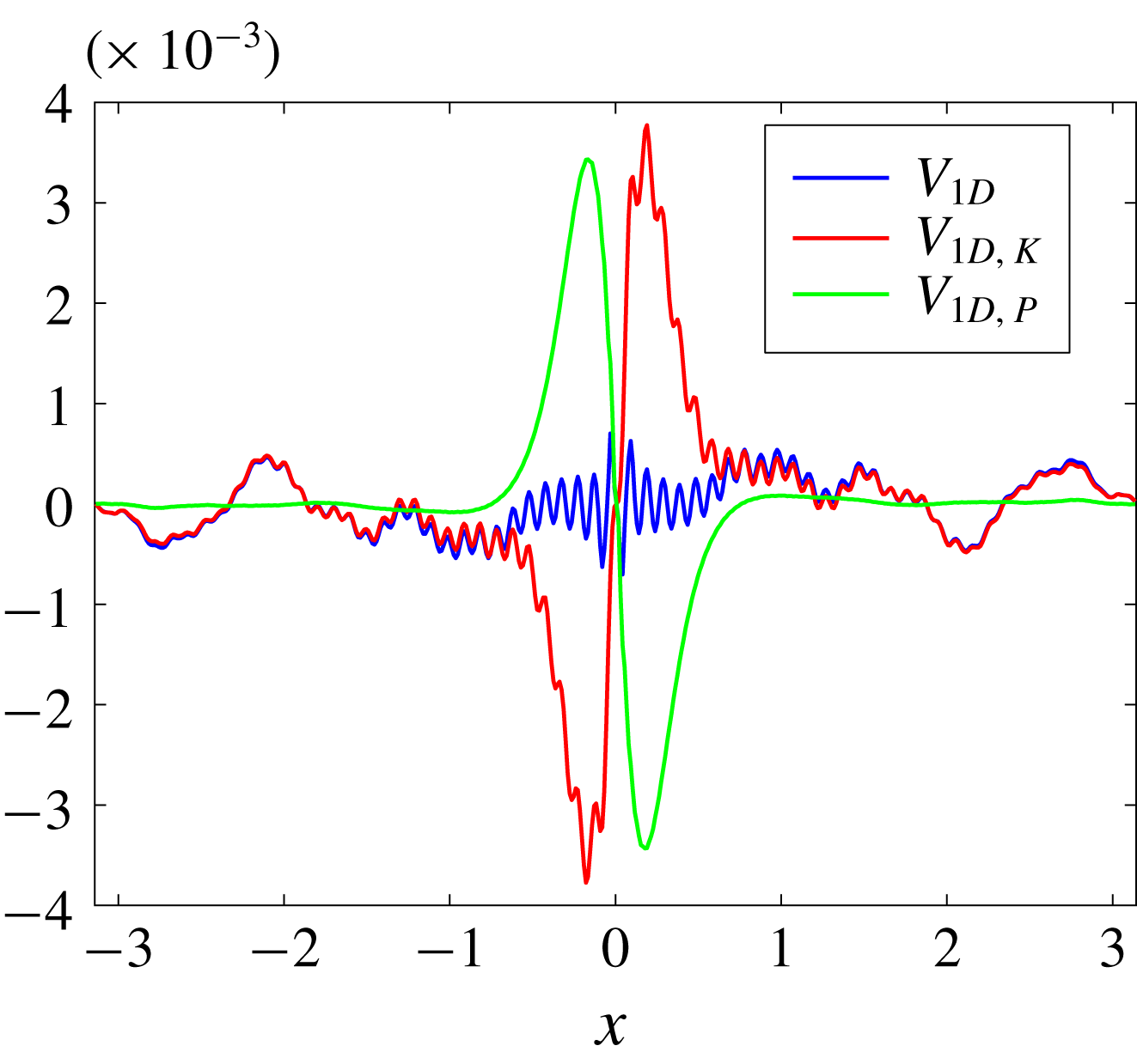
In figure 10 we show the decomposition of
 $V$
into the kinetic and effective potential parts,
 $V_{K}$
and
 $V_{P}$
, respectively. We find that
 $V_{P}$
and
 $V_{K}$
are much larger than their summation
 $V$
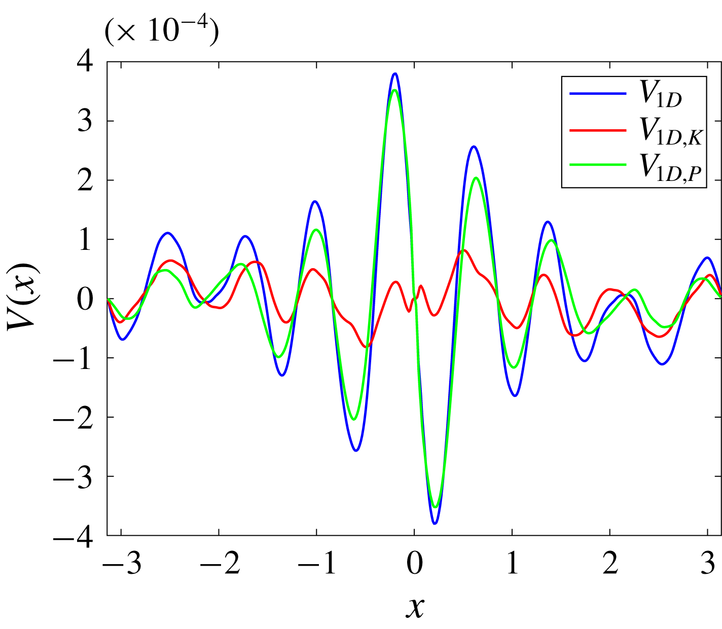
, which consists with the flux-loop scenario that the total energy transfer to small scales is the subtraction of upscale kinetic energy transfer from the downscale potential energy transfer. Clearly, measuring one component is not enough to imply the total energy transfer.
Comparison between the one-dimensional measurement (5.6) and the theoretical result (4.20) for the strong forcing simulation. Panel (b) zooms in on the interval of
 $x\in [-0.4,\,0.4]$
, where the black dashed line represents the local approximation
 $V_{1D}\approx -2\unicode[STIX]{x1D716}x$
for small
 $x$
.

One-dimensional
 $V(x)$
along the
 $x$
-axis and its decompositions
 $V_{K}$
and
 $V_{P}$
.

We now demonstrate the key result from an observational point of view: the spectral energy flux
 $F(K)$
can be recovered accurately from observations of the one-dimensional function
 $V(x)$
. Theoretically, we can obtain
 $F(K)$
from a measured
 $V(x)$
through (e.g. Frisch Reference Frisch1995)
 $$\begin{eqnarray}\displaystyle F(K)=-{\displaystyle \frac{1}{16\unicode[STIX]{x03C0}^{2}}}\int _{0}^{K}\unicode[STIX]{x1D705}\,\text{d}\unicode[STIX]{x1D705}\int _{0}^{2\unicode[STIX]{x03C0}}\,\text{d}\unicode[STIX]{x1D6FC}\left\{\int _{-\infty }^{\infty }\int _{-\infty }^{\infty }\unicode[STIX]{x1D735}\boldsymbol{\cdot }\boldsymbol{V}\text{e}^{-\text{i}\boldsymbol{k}\boldsymbol{\cdot }\boldsymbol{r}}\text{d}x\,\text{d}y\right\}, & & \displaystyle\end{eqnarray}$$
where we first take the Fourier transform of
 $\unicode[STIX]{x1D735}\boldsymbol{\cdot }\boldsymbol{V}$
to obtain the spectral energy transfer function and then integrate it within a disk of radius
 $K$
. After integrating by parts and simplification, (5.7) becomes (cf. (5.8) in Xie & Bühler (Reference Xie and Bühler2018))
 $$\begin{eqnarray}\displaystyle F(K)=-{\displaystyle \frac{K^{2}}{4}}\int _{0}^{\infty }V(r)J_{2}(Kr)\,\text{d}r. & & \displaystyle\end{eqnarray}$$
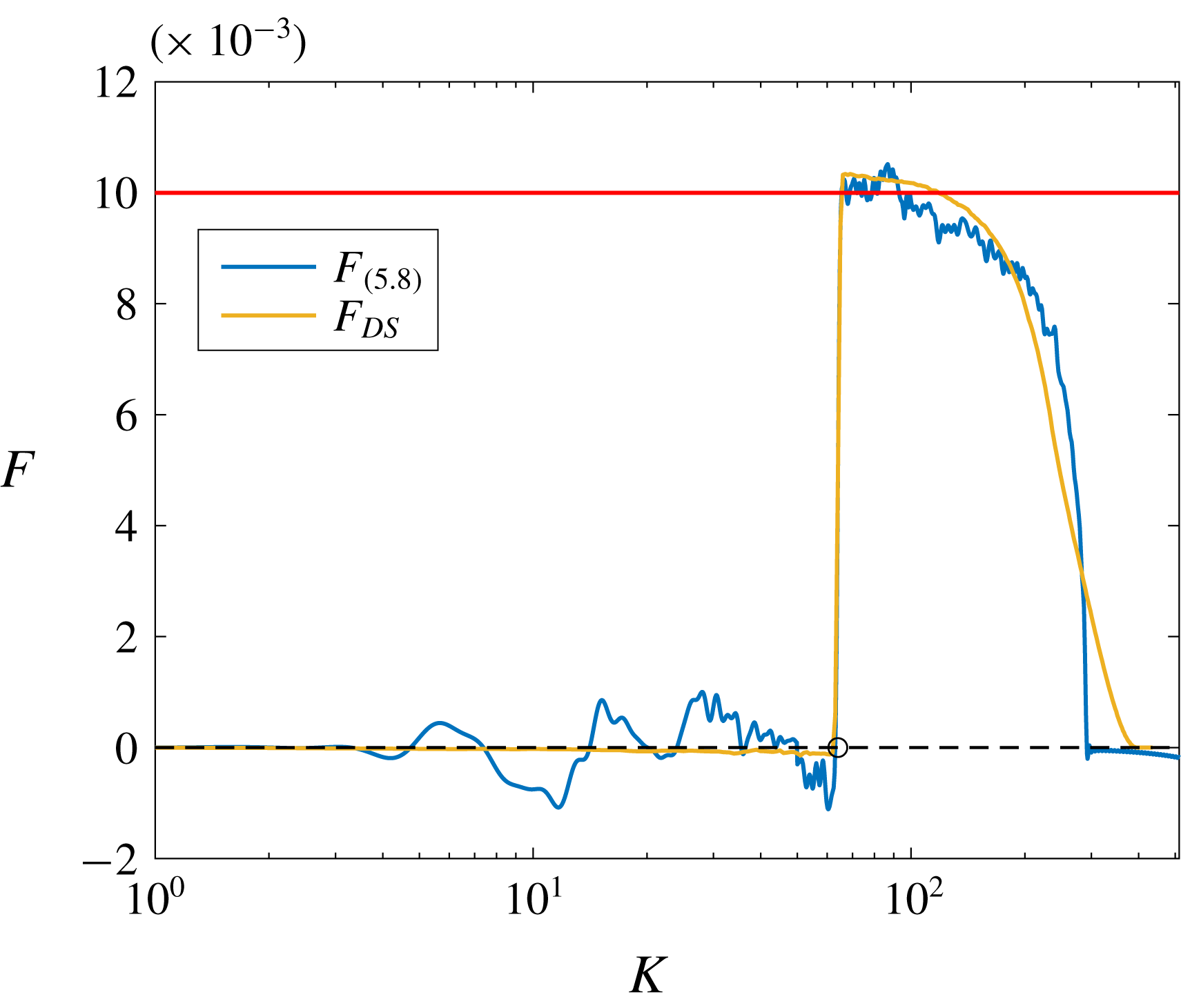
In figure 11 we compare the recovered
 $F(K)$
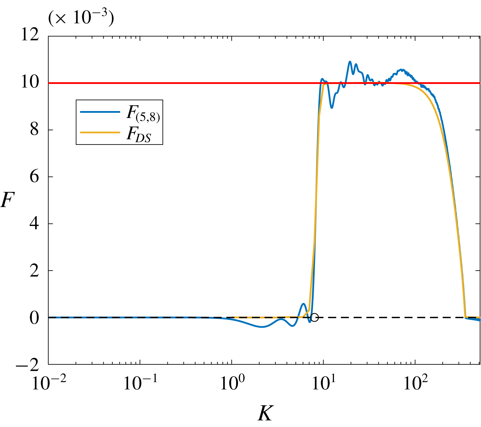
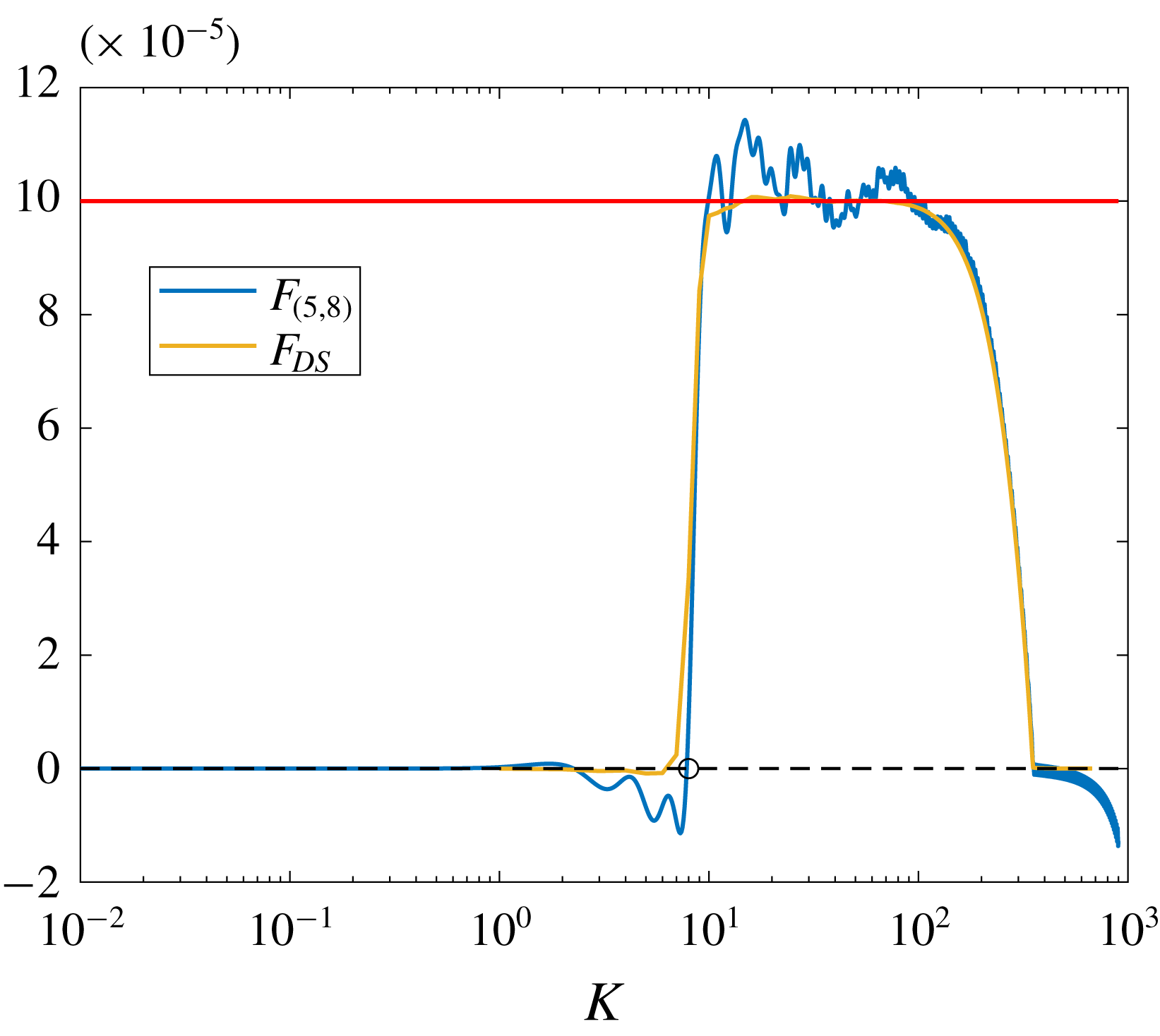
against the exact solution, and clearly both the forcing scale and total energy transfer rate are recovered with acceptable accuracy. In calculating the integration in (5.8) we simply applied the trapezoidal method. Since we know that the Bessel functions are oscillatory, a better algorithm will give us better results. But this simple integration implies that applying expression (5.8) is robust.
Comparison between the spectral total energy flux recovered from the structure function
 $V$
using (5.8)
 $F_{(5.8)}$
and that obtained from direct statistics
 $F_{DS}$
in the strong forcing regime. The red line marks the level of
 $\unicode[STIX]{x1D716}=0.01$
, the circle marks the forcing scale and the black dashed line is the
 $0$
-line for reference.

5.2 Intermediate forcing regime (
$l_{O}\sim l_{f}$
)

In this section we show the results of a simulation with in
 $k_{f}=8$
and
 $\unicode[STIX]{x1D716}=0.01$
in (5.1). Therefore the Ozmidov wavenumber is
 $k_{O}\approx 10$
, which is comparable with
 $k_{f}$
. We show the energy evolution in figure 12. At the final state the kinetic energy, the
 $v$
-potential energy
 $E_{v}$
and the potential energy
 $E_{\unicode[STIX]{x1D703}}$
are statistically steady. In figure 13 we show the snapshots of
 $\unicode[STIX]{x1D735}\unicode[STIX]{x1D713}$
,
 $u$
,
 $M=x+v$
and
 $S=z+\unicode[STIX]{x1D703}$
at time
 $t=100$
. The figures are similar to figure 4, but since we have more wavenumber space below the forcing scale, we see finer small-scale structures. We show the kinetic (
 $F_{K}$
), effective potential (
 $F_{P}$
) and total (
 $F_{tot}=F_{K}+F_{P}$
) energy fluxes flux in figure 14. The potential energy is transferred downscale (red curve); the kinetic energy is mainly transferred upscale with a small amount of downscale transfer at small scales. The total energy – potential plus kinetic energies – transfer shows a clear plateau associated with a downscale flux (yellow curve).
Evolution of the kinetic energy
 $E_{\unicode[STIX]{x1D713}}$
,
 $v$
-potential energy
 $E_{v}$
and potential energy
 $E_{\unicode[STIX]{x1D703}}$
for the intermediate regime.

Snapshots of
 $u$
,
 $w$
,
 $M=x+v$
and
 $S=z+\unicode[STIX]{x1D703}$
at time
 $t=100$
for the intermediate regime.

Kinetic (
 $F_{K}$
), effective potential (
 $F_{P}$
) and total
 $(F_{tot})$
energy fluxes for the intermediate regime. The dashed line is the
 $0$
-line which is plotted for reference, while the circle and cross mark the forcing and Ozmidov wavenumbers, respectively.

Based on figure 7, we can describe the energy path. The energy is injected as kinetic energy, but, since the Ozmidov scale is comparable with the forcing scale, conversion into effective potential energy takes place immediately, and indeed the location of the peak of the conversion term is at
 $K=k_{f}=8$
. The total energy flux is robustly downscale and dominated by the effective potential energy. The kinetic energy follows the downscale transfer somewhat reluctantly, as its own contribution to the energy flux is robustly negative. Interestingly, as indicated by the non-constancy of both fluxes, conversion from effective potential to kinetic energy takes place at all wavenumbers larger than
 $k_{O}$
but less than the dissipation range.
With regard to the structure function, we have checked the isotropy of
 $\unicode[STIX]{x1D735}\boldsymbol{\cdot }\boldsymbol{V}_{K}$
and
 $\unicode[STIX]{x1D735}\boldsymbol{\cdot }\boldsymbol{V}_{P}$
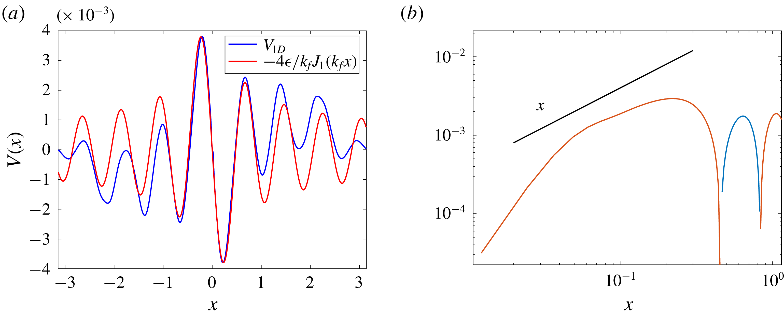
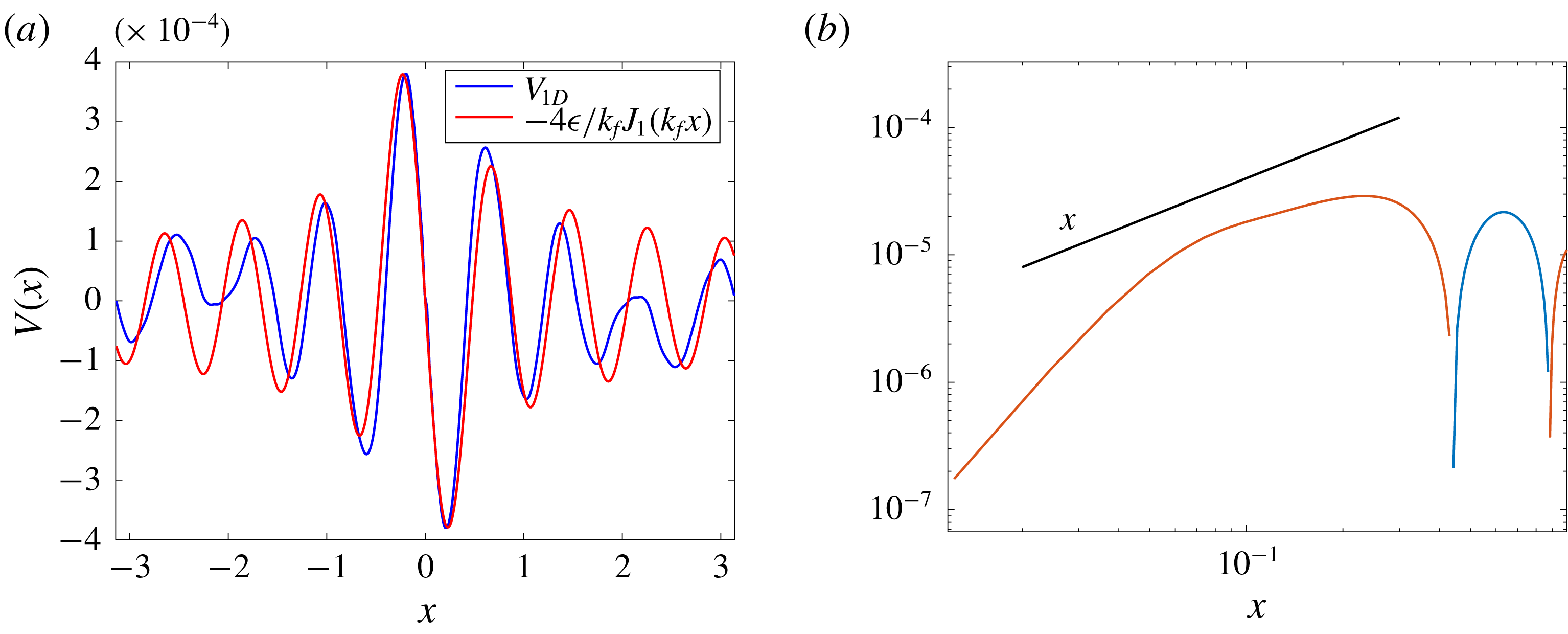
, but since they do not provide us much more information compared with the ones shown in the first numerical simulation (cf. figures 6 and 8.), we do not show them. The comparison between the one-dimensional measurement (5.6) with the theoretical result (4.20) is shown in figure 15. Panel (a), we show that the measurement and the theoretical results match well for several oscillations of the Bessel function, and the panel (b) presents the limiting
 $V\sim -2\unicode[STIX]{x1D716}r$
behaviour for small
 $r$
in a log–log coordinate. We stress that the relation (4.20) provides us more than the commonly used asymptotic linear dependence of
 $V$
on
 $r$
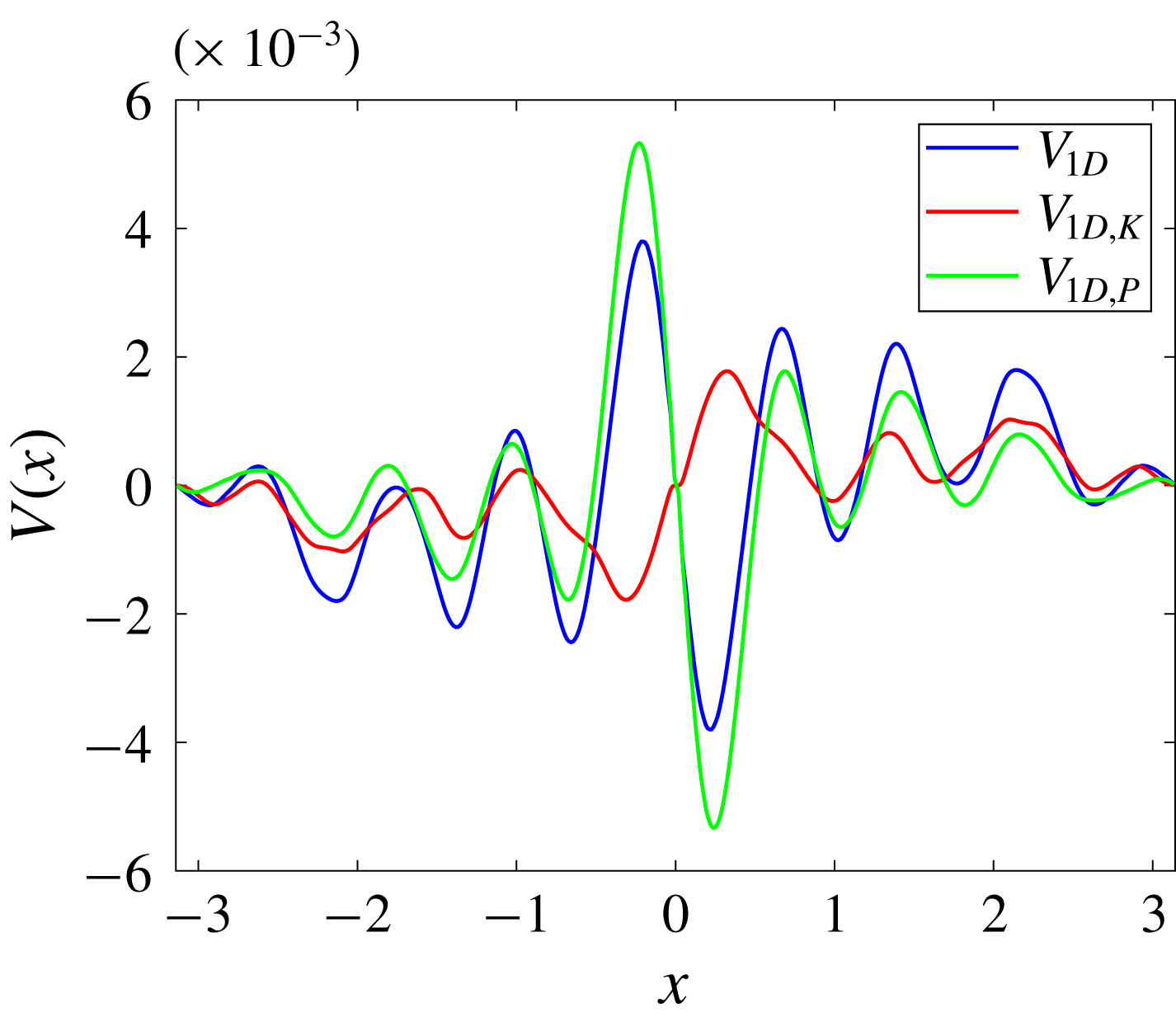
and we should consider the Bessel function structure if the real space measurement is considered. In figure 16 we show the decomposition of
 $V$
into
 $V_{K}$
and
 $V_{P}$
. We find that
 $V_{P}$
is dominant and
 $V_{K}$
presents a opposite sign compared with
 $V$
and
 $V_{P}$
for small
 $x$
. This implies that if we use only the kinetic component to detect the total energy flux, we obtain a qualitatively wrong result. Finally, in figure 17 we show the recovered spectral total energy flux. Both the forcing scale and total energy transfer rate are recovered with acceptable accuracy.
Comparison between the numerical and theoretical results of the one-dimensional
 $V(x)$
expression along the
 $x$
-axis for the intermediate regime. Panel (b) shows a log–log coordinate plot. The red and blue colours denote the negative and positive values, respectively. The black line has the same slope as
 $x$
.

One-dimensional
 $V(x)$
along the
 $x$
-axis and its decompositions
 $V_{K}$
and
 $V_{P}$
for the intermediate regime.

Comparison between the spectral total energy flux recovered from the structure function
 $V$
using (5.8)
 $F_{(5.8)}$
and that obtained from direct statistics
 $F_{DS}$
in the intermediate regime. The red line marks the level of
 $\unicode[STIX]{x1D716}=0.01$
, the circle marks the forcing scale and the black dashed line is the
 $0$
-line for reference.

5.3 Weak forcing regime (
$l_{O}\ll l_{f}$
)

Here
 $k_{f}=8$
and
 $\unicode[STIX]{x1D716}=10^{-4}$
in (5.1), therefore the Ozmidov wavenumber is
 $k_{O}=100$
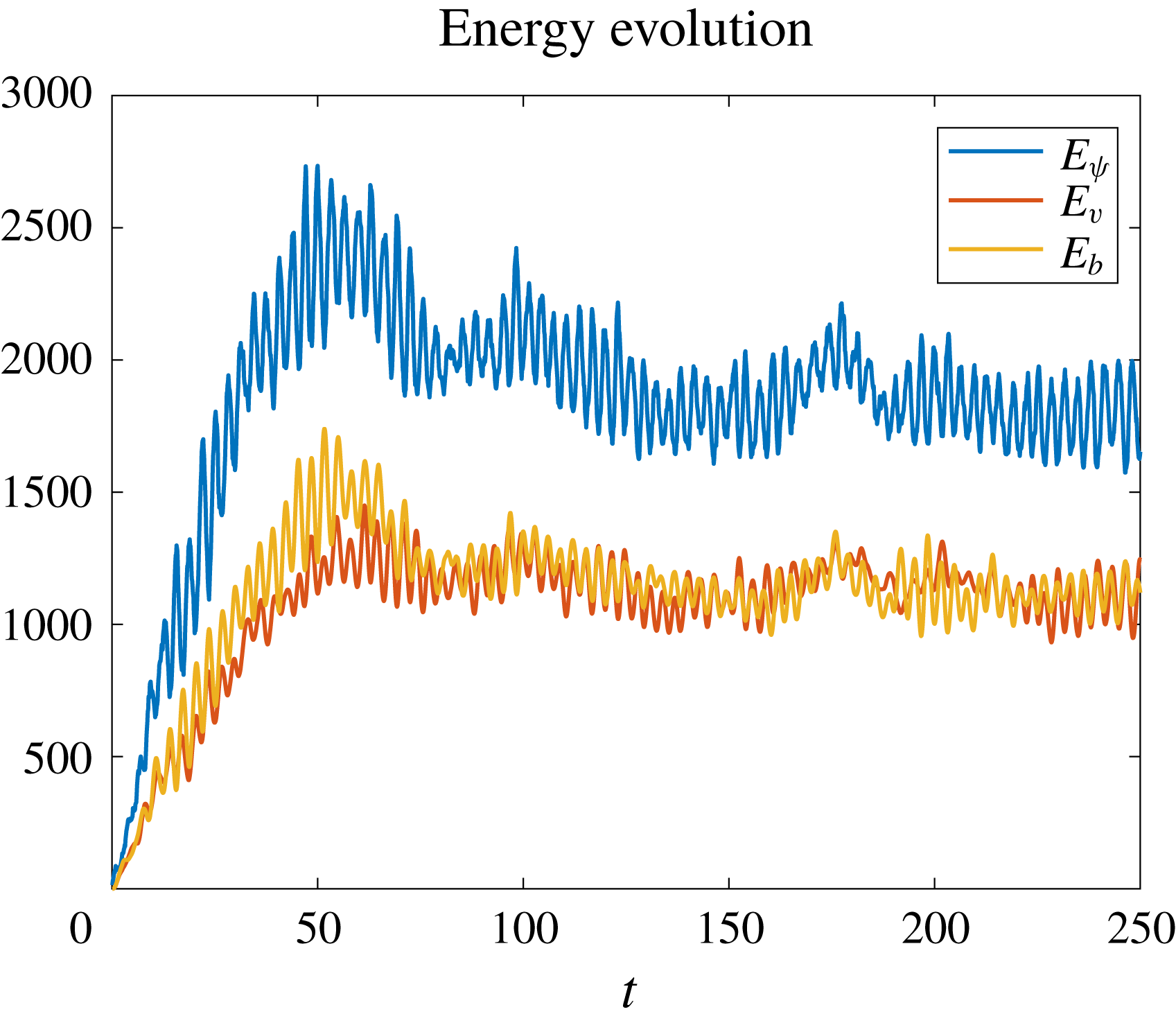
, which is much larger than the forcing wavenumber. We show the energy evolution in figure 18. A major difference between this simulation and the previous two is the clear appearance of linear inertia–gravity oscillation at the only available linear frequency, which is
 $\unicode[STIX]{x1D714}=1$
. This manifests as oscillations between the various energy components at a period around
 $\unicode[STIX]{x03C0}$
, corresponding to twice the wave frequency. Essentially, in this case the forcing is so weak that conversion takes place immediately, and the flow near the forcing scales consists of nearly linear inertia–gravity waves. This is also borne out by the apparent equipartition of energy in figure 18, i.e.
 $E_{\unicode[STIX]{x1D713}}\approx E_{v}+E_{\unicode[STIX]{x1D703}}$
holds, which is consistent with linear waves. In figure 19 we show snapshots of
 $u$
,
 $w$
,
 $x+v$
and
 $z+\unicode[STIX]{x1D703}$
at time
 $t=250$
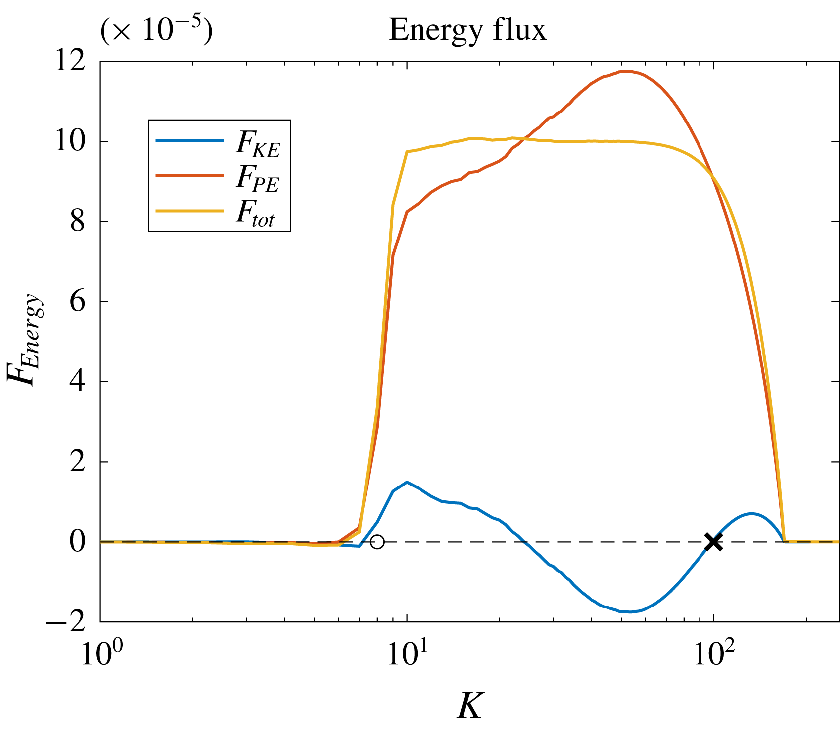
and the energy fluxes are depicted in figure 20. The effective potential energy is again transferred downscale (red curve), but the direction of the kinetic energy change now depends on wavenumber (blue curve). A heuristic explanation for this is as follows. Far below the Ozmidov wavenumber weakly nonlinear wave dynamics is dominant and the fluxes of both potential and kinetic energy are therefore synchronized and downscale. Then, as the Ozmidov wavenumber is approached, the flow loses its nearly linear synchronization and the previously observed intrinsic upscale flux tendency of the kinetic energy can manifest itself. The comparison between the one-dimensional measurement (5.6) with the theoretical result (4.20) is shown in figure 21. Since we only measure the total energy flux, based on (4.20) the results are identical to those of the
 $l_{O}\sim l_{f}$
case (cf. figure 15), but of a different magnitude. Figure 22 shows the decomposition of
 $V$
into the kinetic and effective potential parts,
 $V_{K}$
and
 $V_{P}$
, respectively.
In figure 23 we show the recovered spectral total energy flux.
Evolution of the kinetic energy
 $E_{\unicode[STIX]{x1D713}}$
,
 $v$
-potential energy
 $E_{v}$
and potential energy
 $E_{\unicode[STIX]{x1D703}}$
for the case with
 $l_{O}\ll l_{f}$
.

Snapshots of
 $u$
,
 $w$
,
 $x+v$
and
 $z+\unicode[STIX]{x1D703}$
at time
 $t=100$
for the case with
 $l_{O}\ll l_{f}$
.

Kinetic (
 $F_{K}$
), effective potential (
 $F_{P}$
) and total
 $(F_{tot})$
energy fluxes. The dashed line is the
 $0$
-line which is plotted for reference; the circle and cross mark the forcing and Ozmidov wavenumbers, respectively.

Comparison between the numerical and theoretical result of the one-dimensional
 $V(x)$
expression along the
 $x$
-axis in the weak forcing regime. Panel (b) shows a log–log coordinate plot. The red and blue colours denote the negative and positive values, respectively. The black line has the same slope as
 $r$
.

One-dimensional
 $V(x)$
along the
 $x$
-axis and its decompositions
 $V_{K}$
and
 $V_{P}$
in the weak forcing regime.

Spectral total energy flux recovered from the structure function
 $V$
using (5.8) for the weak forcing regime simulation. The red line marks the level of
 $\unicode[STIX]{x1D716}=10^{-4}$
.

5.4 Control run with PV forcing
In the previous three simulations we did not force the PV, so the flow regimes were all versions of wave turbulence. Forcing the PV in a three-dimensional simulation would greatly affect the solution, but, as discussed before, in the two-dimensional case the balanced flow has essentially no intrinsic dynamic evolution of its own. The robustness of the two-dimensional wave turbulence picture is confirmed here with a simulation that allows for additional forcing of PV. We illustrate that the downward total energy transfer remains robust, and occurs regardless of the specific forcing components. This simulation uses all the parameters of the strong forcing regime experiment in § 5.1, except that we add additional external buoyancy forcing
 $F_{v}$
and
 $F_{b}$
(cf. (4.1)) and set the total potential energy input rate equals
 $0.005$
, one half of the kinetic energy input rate
 $\unicode[STIX]{x1D716}=0.01$
.
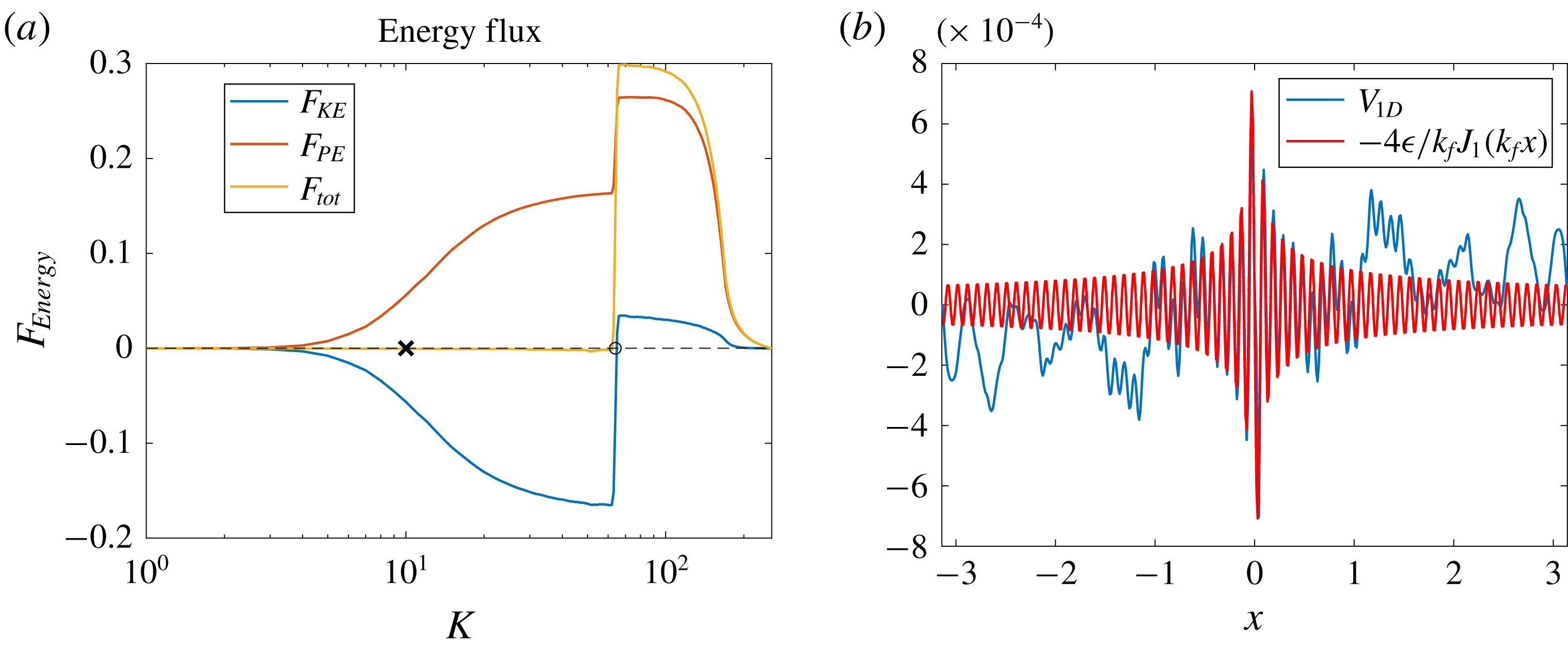
In figure 24 we show the spectral energy flux and one-dimensional structure function
 $V(x)$
in this simulation. In panel (a) we find that the energy flux-loop scenario remains: the input kinetic energy is first transferred upscale, then it is converted to the potential energy, which fluxes downscale. The conversion happens around the Ozmidov scale, which should now be estimated using the kinetic energy input rate and is therefore the same as that in the vortex experiment (
 $k_{O}\approx 10$
). Below the forcing scale, the downscale potential energy flux consists of two part, one is the converted kinetic energy and the other is the direct input of potential energy from the external forcing. In the right panel we confirm that the theoretical expression (4.20) remains valid due to the downscale total energy transfer. We also checked the intermediate and weak forcing regimes with additional buoyancy forcing, and they both show total energy transfer downscales. But because that they are less complicated compared with the flux-loop scenario, we do not show them in the text.
Energy fluxes (a) and the comparison between the numerical and theoretical result of the one-dimensional
 $V(x)$
expression along the
 $x$
-axis (b) for the case with PV forcing. The circle and the cross mark the forcing and Ozmidov scales, respectively.

6 Multiple forcing scales
For standard two-dimensional isotropic turbulence Xie & Bühler (Reference Xie and Bühler2018) showed how to compute both the longitudinal and transversal third-order velocity structure functions exactly, which when summed up yield the total
 $V(r)$
. This quite complete theory allowed some simple robust diagnostics to be formulated that allowed sharpening the estimates of spectral energy fluxes in the presence of multiple forcing scales, in which case energy and enstrophy cascade regions can overlap. Essentially, by using particular linear combinations of the longitudinal and transversal structure functions it was possible to filter out the enstrophy flux terms and highlight the energy flux terms.
In the present case there is no enstrophy flux, which simplifies the situation, but on the other hand we do not have a theory for the individual constituents of
 $V(r)$
in § 4, which complicates matters. Still, we can make use of the exact Bessel function form of
 $V(r)$
. Now, as shown in Xie & Bühler (Reference Xie and Bühler2018), for scales larger than the forcing scale in two-dimensional turbulence, the Bessel correction is of high order compared with the
 $r$
dependence due to the inverse cascade, however, in our present set-up the Bessel function dominates the large scale, so making use of the Bessel function is unavoidable. Here, we show two methods of determining the forcing scale and energy input strength in the configuration space and spectral space, respectively.
6.1 Configuration space detection
We consider an idealized experiment with external forcing at three wavenumbers
 $k_{1}=10$
,
 $k_{2}=10^{3}$
and
 $k_{3}=10^{5}$
with equal energy input rate
 $\unicode[STIX]{x1D716}_{1}=\unicode[STIX]{x1D716}_{2}=\unicode[STIX]{x1D716}_{3}=1$
. The theoretical result (4.20) indicates that the forcing at each scale contribute to the structure function by
 $V_{i}=-4\unicode[STIX]{x1D716}_{i}J_{1}(k_{i}x)$
, so the total structure function can be expressed as
 $V=\sum _{i=1}^{3}V_{i}$
. Based on the expansion of
 $J_{1}$
we plot
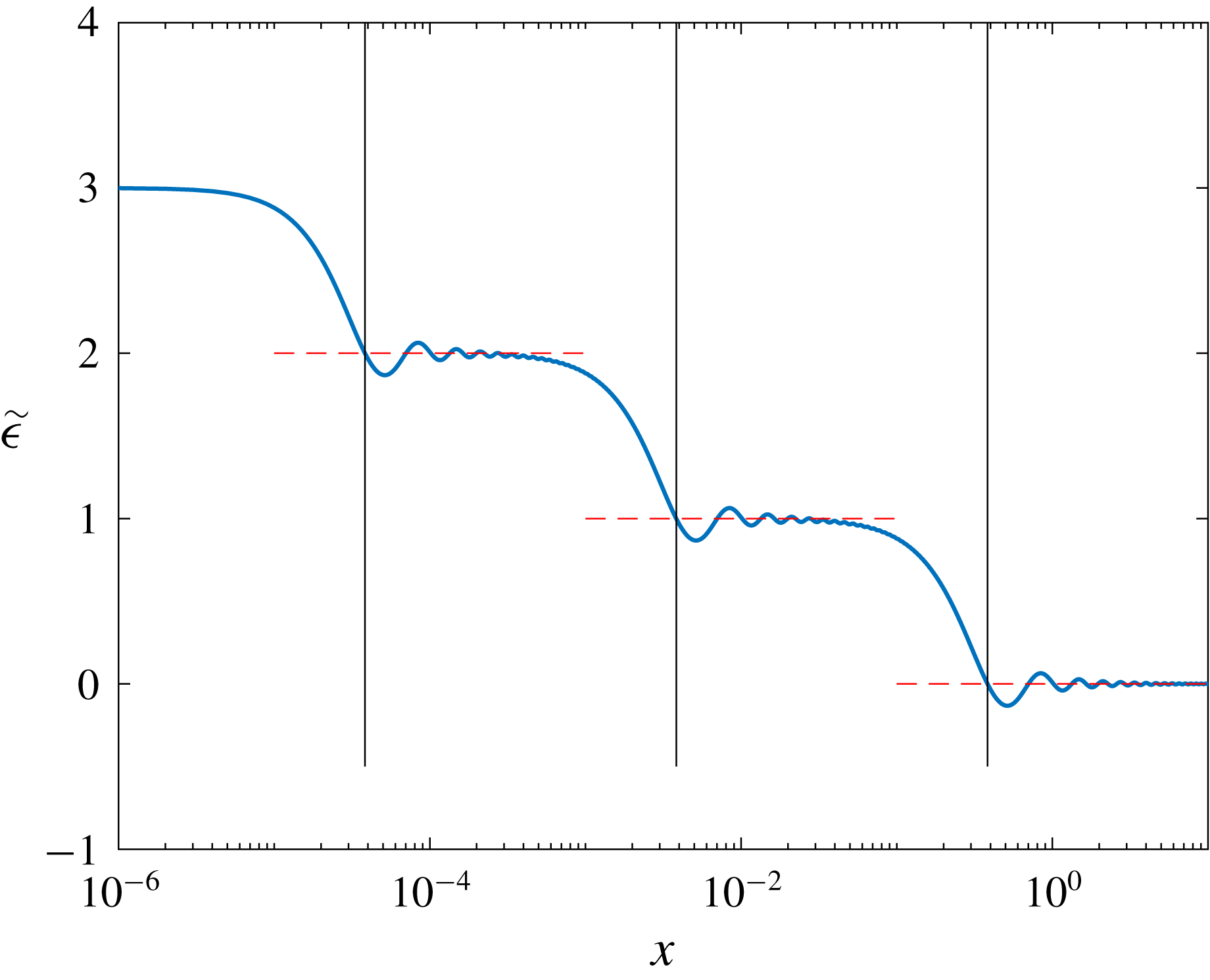
 $\tilde{\unicode[STIX]{x1D716}}=-V/(2x)$
in figure 25, where the height of plateaus indicates the energy input rate below this scale. e.g. in this figure we observe four plateaus with height
 $3$
,
 $2$
,
 $1$
and
 $0$
, and the second plateau implies that below this scale the energy input rate is
 $2$
, which equals
 $\unicode[STIX]{x1D716}_{1}+\unicode[STIX]{x1D716}_{2}$
.
However, it is not so easy to determine what is the forcing wavenumber (scale) since the transitions between plateaus expand over a decade. Now the Bessel oscillation gives us an advantage that it has zero points, based on which we propose to use the value of the plateaus and the first zero of
 $J_{1}(x)$
,
 $x=a_{1}=3.8317$
, to determine the forcing wavenumber: we extend the plateau value to its left and find the leftmost intersection with the
 $\tilde{\unicode[STIX]{x1D716}}$
curve, then we can calculate the forcing wavenumber using the
 $x$
value of the intersection point by
 $a_{1}/x$
. We check this approach in figure 25 by the solo intersection of the blue, red and black curves.
Log-normal plot of
 $\tilde{\unicode[STIX]{x1D716}}=-V/(2x)$
for an equal-strength external forcing at wavenumbers
 $k_{1}=10$
,
 $k_{2}=10^{3}$
and
 $k_{3}=10^{5}$
. The red dashed lines have vertical values equal to those of the plateaus. The vertical back lines have horizontal coordinates equal to
 $a_{1}/k_{i}$
with
 $a_{1}$
the first non-zero zero of
 $J_{1}$
.

We want to note that the negative value of
 $\tilde{\unicode[STIX]{x1D716}}$
in figure 25 does not indicate a change in the direction of energy flux, and, in fact, the direction of total energy transfer is downscale for the whole range.
6.2 Spectral space detection
The advantage of detection in the configuration space is that we can use the directly measurable quantities. However, due to the oscillatory nature of the Bessel function, when two forcing scales are close it is hard to separate their effects on the measurable third-order structure function
 $V$
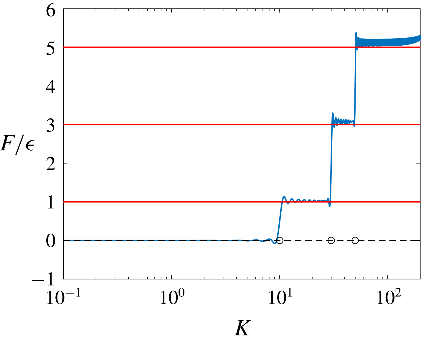
. In this section, we propose using (5.8) to detect forcing scales and energy input rate in the spectral space. This method involves processing the measured date with an integration, whose accuracy will depend on the noise level of the measured data, but as we show in the numerical simulations, equation (5.8) can robustly detect the forcing scale sharply, which enables us to deal with the situations with close forcing scales.
We consider an artificial forcing at three scales
 $k_{f}=10,30$
and
 $50$
with strength
 $\unicode[STIX]{x1D716},2\unicode[STIX]{x1D716}$
and
 $2\unicode[STIX]{x1D716}$
, respectively. So the corresponding structure function is
 $$\begin{eqnarray}\displaystyle V=-4\unicode[STIX]{x1D716}{\textstyle \frac{1}{10}}J_{1}(10r)-8\unicode[STIX]{x1D716}{\textstyle \frac{1}{30}}J_{1}(30r)-8\unicode[STIX]{x1D716}{\textstyle \frac{1}{50}}J_{1}(50r). & & \displaystyle\end{eqnarray}$$
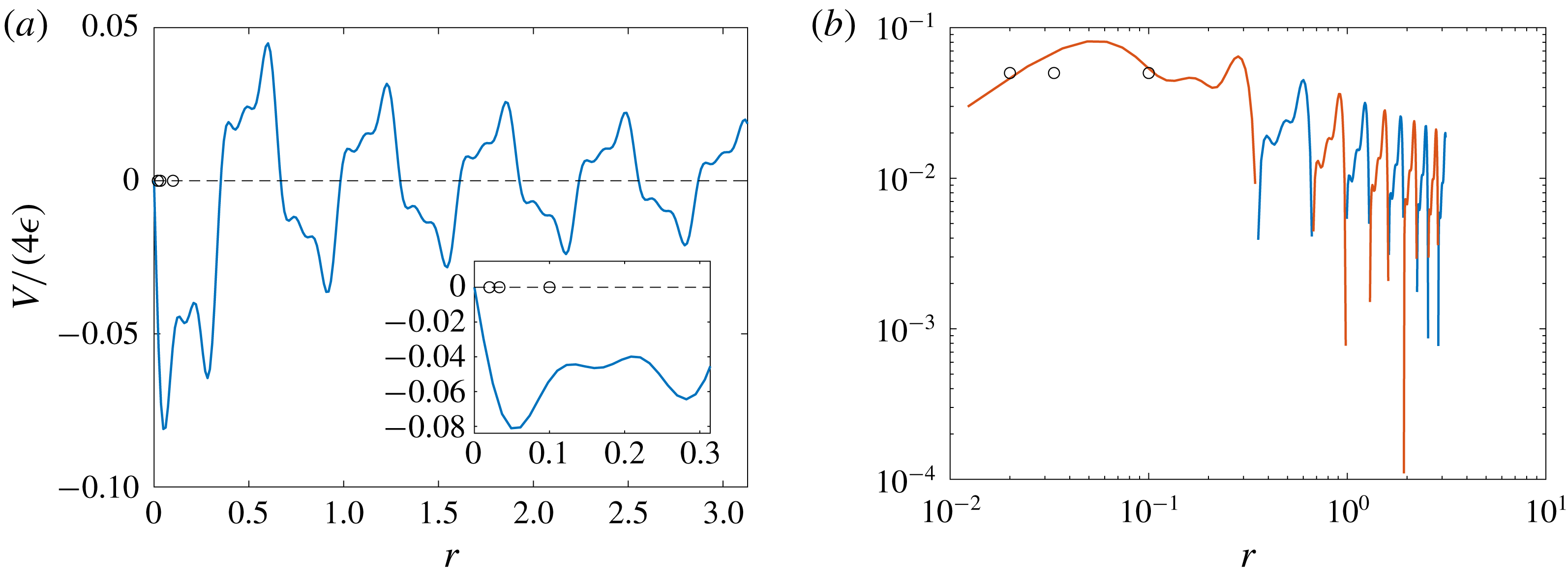
First, figure 26 shows that it is hard to determine the forcing scales and the corresponding energy inputs by simply plotting (6.1) in the configuration space. Even though in panel (b) we can find the total energy flux by matching the small-
 $r$
slope, but no detailed information of external forcing at each forcing scale can be obtained.
Structure function for the toy model (6.1). The circles mark the forcing scales
 $1/10$
,
 $1/30$
and
 $1/50$
. The inset in (a) zooms in on the region around forcing scales. In panel (b) the blue and red curves mark the positive and negative values, respectively.

In figure 27 we show that using (5.8) both the forcing scales and corresponding energy inputs can be well detected. So we conclude that if the accuracy of measurements permits, it is better to apply (5.8) to detect the external forcing information from the spectral space.
Energy flux of the toy model obtained from structure function. The red lines mark energy-flux levels
 $1$
,
 $3$
and
 $5$
; the circles mark the forcing scales
 $10$
,
 $30$
and
 $50$
.

7 Concluding comments
Our primary goal in this paper has been to extend the classical structure function theory towards applicability in highly nonlinear rotating stratified flow, and we achieved that goal within the confines of our peculiar two-dimensional isotropic model of inertia–gravity wave turbulence. Despite its simplicity, this system exhibited an interesting range of behaviours as a function of the forcing strength. Essentially, the behaviour of the system was strongly nonlinear at wavenumbers above the Ozmidov wavenumber
 $k_{O}$
, which in the strong forcing case allowed for significant upscale flux of the in-plane kinetic energy. This occurred because of the approximate conservation of
 $y$
-vorticity at the strongly nonlinear wavenumbers above
 $k_{O}$
. This is of course very different from the exact conservation of balanced PV in three-dimensional rotating stratified turbulence (cf. Alexakis & Biferale Reference Alexakis and Biferale2018).
At and below
 $k_{O}$
the dynamics becomes increasingly more linear, and significant conversion of kinetic to effective potential energy can take place. Once excited, the effective potential energy flux was robustly downscale and that led to the overall downscale flux of energy observed in all cases. This makes clear that a downscale wave energy flux is not confined to small-amplitude weak wave turbulence, but occurs at large amplitude as well, provided the domain is large enough to accommodate the Ozmidov scale. Interestingly, our third simulation with weak forcing is close to the regime of weak wave theory. Due to the peculiar dispersion relation
 $\unicode[STIX]{x1D714}^{2}=1$
there can be no resonant triad interactions, but resonant quartets are plentiful, and could presumably be studied using methods from weak surface wave turbulence.
From a theoretical point of view, we derived the exact inviscid solution
 $$\begin{eqnarray}\displaystyle V(r)=-{\displaystyle \frac{4}{r}}\int _{0}^{r}P(s)s\,\text{d}s & & \displaystyle\end{eqnarray}$$
for the third-order structure function away from the dissipation range. At first sight this solution mimics the one obtained by Xie & Bühler (Reference Xie and Bühler2018), but the opposite directions of the energy flux distinguishes the two: in the range of scales larger than the forcing scale, the third-order structure function of two-dimensional turbulence shows a linear dependence on the displacement
 $r$
with small oscillations, while in the two-dimensional rotating stratified turbulence, it is dominated by the Bessel function and therefore is not sign definite, which is similar to that in the three-dimensional turbulence. Such forcing-scale-resolving expressions are important for their potential applications to geophysical flows, where the forcing scales vary a lot due to very distinct mechanisms that are in play.
Here we feel that a crucial puzzle piece is given by the expression
 $$\begin{eqnarray}\displaystyle F(K)=-{\displaystyle \frac{K^{2}}{4}}\int _{0}^{\infty }V(r)J_{2}(Kr)\,\text{d}r,\quad & & \displaystyle\end{eqnarray}$$
which relates the spectral energy flux
 $F(K)$
and the structure function
 $V(r)$
. In principle, from this relation one can detect the scales of the external forcing and the corresponding energy inputs based on using measured third-order structure functions. It is interesting to note that (5.8) can be inverted exactly to yield
 $$\begin{eqnarray}\displaystyle V(r)=-4r\int _{0}^{\infty }{\displaystyle \frac{1}{K}}F(K)J_{2}(Kr)\,\text{d}K. & & \displaystyle\end{eqnarray}$$
So this equation enables the calculation of the structure function
 $V(r)$
from a prescribed energy flux
 $F(K)$
, albeit in a manifestly non-local manner. For example, consider a situation with bidirectional energy transfer such that
 $$\begin{eqnarray}\displaystyle F(K)=-\unicode[STIX]{x1D716}_{u}+(\unicode[STIX]{x1D716}_{u}+\unicode[STIX]{x1D716}_{d})H(K-k_{f}), & & \displaystyle\end{eqnarray}$$
where
 $\unicode[STIX]{x1D716}_{u}$
and
 $\unicode[STIX]{x1D716}_{d}$
are the magnitudes of the upscale and downscale energy fluxes and
 $k_{f}$
is the forcing wavenumber. Then (7.1) gives
 $$\begin{eqnarray}\displaystyle V(r)=2\unicode[STIX]{x1D716}_{u}r-4{\displaystyle \frac{\unicode[STIX]{x1D716}_{u}+\unicode[STIX]{x1D716}_{d}}{k_{f}}}J_{1}(k_{f}r), & & \displaystyle\end{eqnarray}$$
which describes a reasonable form for the structure function in a two-dimensional bidirectional energy transfer turbulence. And we can easily check that taking
 $\unicode[STIX]{x1D716}_{u}=0$
or
 $\unicode[STIX]{x1D716}_{d}=0$
, equation (7.3) recovers the results of two limiting cases with unidirectional energy transfer, which are studied in this present paper (cf. (4.20)) and Xie & Bühler (Reference Xie and Bühler2018) (cf. (4.9b) therein).
We want to stress again that expressions such as (5.8) and (7.1) are non-local in
 $K$
and
 $r$
. They contrast to previous theories (cf. Kolmogorov Reference Kolmogorov1941; Bernard Reference Bernard1999) where the structure functions are described by a power function of the displacement
 $r$
in limiting inertial ranges, which makes it hard to glue the piecewise expressions in different ranges together to obtain a global, uniformly valid expression. In application, such an expression that applies to a wide range is useful: when the power laws are not obvious, the obtained exponents depend on the measured range, but matching a wide-range expression does not have this problem. In addition, it can make use of the data between the power-law regions! For example, bidirectional total energy transfer is observed in confined rotating turbulence (Deusebio et al.
Reference Deusebio, Boffetta, Lindborg and Musacchio2014b
) and magnetohydrodynamic turbulence (Marino et al.
Reference Marino, Sorriso-Valvo, Carbone, Noullez, Bruno and Bavassano2008, Reference Marino, Sorriso-Valvo, D’Amicis, Carbone, Bruno and Veltri2012; Seshasayana, Benavides & Alexakis Reference Seshasayana, Benavides and Alexakis2014; Seshasayana & Alexakis Reference Seshasayana and Alexakis2016) and ongoing work indicates that (7.3) appears quantitatively useful in this application.
Acknowledgements
We thank the reviewers of this manuscript, whose comments greatly improved our presentation. We gratefully acknowledge financial support from the United States National Science Foundation grant DMS-1312159 and Office of Naval Research grant N00014-15-1-2355.