1. Introduction
Shock/turbulence interactions are of interest in many areas of science and engineering. Emission of vortical, acoustic and entropic waves behind the shock can be precipitated either by local upstream disturbances impinging upon the shock or by a more distant mechanism such as the unsteady motion of a shock foot, which sends ripples along the length of the shock and causes emission of disturbances unrelated to the local upstream flow features. The general case is too complex to describe using current theoretical models, but the shock interaction of local upstream disturbances can be isolated from the more distant effects by considering a canonical shock/isotropic turbulence interaction (SITI): a nominally planar normal shock interacting with an isotropic incident disturbance field.
The SITI problem has been studied via experiments, numerical simulations and analytical methods. The geometry is convenient for numerical simulations and for analytical studies but difficult to reproduce in a laboratory experiment. In addition, the interaction is quite sensitive to the details of the incident fluctuations, about which much more can be known and controlled in simulations and theory than in the laboratory. In particular, very different post-shock fluctuations are produced depending on whether the incident velocity fluctuations are dilatational or vortical in nature. Therefore, measuring the level of velocity fluctuations in an experiment is not sufficient to fully specify the problem. Unwanted or unexpected sound waves from, for example, the passage of a shock wave along the turbulent wall layers in a shock tube could significantly alter the results of an experiment intended to investigate solenoidal incident turbulence. A review of experiments prior to 2000 is given by Andreopoulos, Agui & Briassulis (Reference Andreopoulos, Agui and Briassulis2000), and Agui, Briassulis & Andreopoulos (Reference Agui, Briassulis and Andreopoulos2005) reported further experimental work on the SITI problem. A discussion of the difficulties involved in producing the desired geometry and incident field as well in interpreting the results can be found in Smits & Dussauge (Reference Smits and Dussauge2006). A number of qualitative discrepancies exist between the experiments and theoretical results; however, the agreement is much better between numerical simulations and theory. Because the geometry is conducive to numerical and theoretical study and because of the good agreement that has emerged between these two in the literature, we use numerical simulation data as the basis for comparison in this work.
The SITI problem has been studied at selected conditions using direct numerical simulation (DNS) (Lee, Lele & Moin Reference Lee, Lele and Moin1991, Reference Lee, Lele and Moin1993, Reference Lee, Lele and Moin1997; Hannappel & Friedrich Reference Hannappel and Friedrich1995; Mahesh, Lele & Moin Reference Mahesh, Lele and Moin1997; Jamme et al. Reference Jamme, Cazalbou, Torres and Chassaing2002; Larsson & Lele Reference Larsson and Lele2009; Larsson, Bermejo-Moreno & Lele Reference Larsson, Bermejo-Moreno and Lele2013; Chen & Donzis Reference Chen and Donzis2019; Grube & Martín Reference Grube and Martín2021).
A less costly approach is to apply first-order perturbation theory (Ribner Reference Ribner1954a,Reference Ribnerb; Mahesh et al. Reference Mahesh, Lele and Moin1997); this has become known as linear interaction analysis (LIA). DNS studies by Ryu & Livescu (Reference Ryu and Livescu2014) and Tian et al. (Reference Tian, Jaberi, Li and Livescu2017) have concluded that, in the limit of small fluctuation strength, DNS and LIA results converge both for shock-resolving and shock-capturing simulations, respectively.
Other recent studies have explored related topics in the context of SITI such as mixing of passive scalars (Boukharfane, Bouali & Mura Reference Boukharfane, Bouali and Mura2018; Gao, Bermejo-Moreno & Larsson Reference Gao, Bermejo-Moreno and Larsson2020), variable density and multi-fluid flows (Tian et al. Reference Tian, Jaberi, Li and Livescu2017; Tian, Jaberi & Livescu Reference Tian, Jaberi and Livescu2019), reacting shock waves (Huete et al. Reference Huete, Jin, Martínez-Ruiz and Luo2017) and specialized studies on post-shock thermodynamic fluctuations (Sethuraman, Sinha & Larsson Reference Sethuraman, Sinha and Larsson2018; Sethuraman & Sinha Reference Sethuraman and Sinha2020a,Reference Sethuraman and Sinhab), temperature–velocity correlations (Quadros, Sinha & Larsson Reference Quadros, Sinha and Larsson2016a) and turbulent energy flux (Quadros, Sinha & Larsson Reference Quadros, Sinha and Larsson2016b) to inform turbulence model development.
Even at substantial fluctuation levels, LIA successfully predicts the amplification of turbulence kinetic energy across the shock (Lee et al. Reference Lee, Lele and Moin1997; Larsson & Lele Reference Larsson and Lele2009); however, above approximately Mach 2, it also predicts a post-shock Reynolds stress tensor with the transverse components greater than the streamwise, whereas experiment (Barre, Alem & Bonnet Reference Barre, Alem and Bonnet1996) and DNS exhibit the opposite behaviour.
Some forty-five years after the initial publication of his pioneering work on LIA, Ribner (Reference Ribner1998) reflected on the state of agreement between DNS, experiment and LIA theory. He noted that this discrepancy in the Reynolds stress anisotropy between LIA predictions and the findings of experiment and DNS ‘remain[ed] a puzzle’. The nonlinear terms, which are neglected in LIA, might be expected to cause a return to isotropy downstream of the shock. Why, then, does the Reynolds stress tensor overshoot isotropy and settle into a state with the opposite sense of anisotropy? In order to investigate this question, we augment LIA with an eddy viscosity-based model for the nonlinear interactions between vortical modes in the post-shock region.
The paper is organized as follows: possible causes for the anisotropy discrepancy are catalogued and discussed in § 2. Of these, the only viable candidate is explored in § 3 to qualitatively explain the discrepancy. In § 4 a quantitative model is developed based on the new understanding of the flow physics. In § 5 the model predictions are compared with DNS data to show that the effects in question are both qualitatively and quantitatively suited to cause the observed anisotropy.
2. Possible sources of anisotropy discrepancy
This section catalogues and assesses possible causes for the discrepancy in post-shock Reynolds stress anisotropy between DNS and LIA. The violation of any of the assumptions inherent in LIA theory might be a candidate cause for the discrepancy.
2.1. Production via mean-flow gradients
DNS results of SITI (Lee et al. Reference Lee, Lele and Moin1993; Larsson & Lele Reference Larsson and Lele2009; Grube & Martín Reference Grube and Martín2021) show that the Favre-averaged velocity (or, equivalently, mean density, since the two are reciprocals) varies with distance from the shock. This raises the possibility of creating anisotropy through the production terms in the Reynolds stress budget; however, the deviation of the post-shock mean flow from its classical Rankine–Hugoniot value is of second order in the perturbation strength. One would therefore expect a much smaller discrepancy in the anisotropy for lower turbulence Mach numbers,  $M_t$. However, in the DNS of Larsson et al. (Reference Larsson, Bermejo-Moreno and Lele2013), no
 $M_t$ dependence is perceptible at Mach 3.5 where the anisotropy discrepancy is quite large.
2.2. Viscous terms
Linear analyses in the literature are, to the authors’ knowledge, all inviscid. Using refraction laws to link pre- and post-shock wavelengths of elementary (Fourier) vortical waves, one can see that the post-shock viscous decay of the LIA-predicted emitted vorticity would produce anisotropy in the sense that is observed in DNS and experiment ( $R_{11}>R_{22}$). However, this prediction is reliable only to the extent that the post-shock solution evolves linearly. If nonlinear effects are important to the evolution of the post-shock vorticity field, then the actual post-shock field will rapidly depart from the LIA prediction and computing viscous terms from the LIA solution will not yield useful information. Indeed, this appears to be the case since the anisotropy data reported by Larsson et al. (Reference Larsson, Bermejo-Moreno and Lele2013), for example, show little if any dependence of the anisotropy on the Reynolds number. If the mechanism were viscous (and hence essentially linear in nature), then the effect should be inversely proportional to the Reynolds number.
Another effect of viscosity is the modification of the jump conditions at the shock. A viscous linear analysis (not shown) indicates that the turbulence amplification at the shock is indeed modified in a way that favours  $R_{11}$ over
 $R_{22}$, but this effect is too small to account for the observed discrepancy. And again, if viscous effects were responsible for the discrepancy through their influence on the turbulence amplification, then an inverse
 $Re$ dependence would be evident. We therefore conclude that viscosity is not a major contributor to the Reynolds stress anisotropy.
2.3. Nonlinear terms
In the case of incident vortical turbulence, LIA results (Ribner Reference Ribner1954b; Mahesh et al. Reference Mahesh, Lele and Moin1997) show that beyond a downstream distance of approximately one half the dissipation length scale  $L=TKE^{3/2}/\epsilon$ of the incident field, virtually all of the post-shock turbulent kinetic energy (TKE) is attributable to the vortical field. Here,
 $TKE=R_{jj}/2$ and
 $\epsilon$ is the rate of dissipation of TKE. The good agreement reported in the literature between LIA predictions of these vortical modes and DNS TKE results extrapolated from the post-shock region to the mean shock location (Lee et al. Reference Lee, Lele and Moin1997; Mahesh et al. Reference Mahesh, Lele and Moin1997; Larsson & Lele Reference Larsson and Lele2009; Larsson et al. Reference Larsson, Bermejo-Moreno and Lele2013; Grube & Martín Reference Grube and Martín2021) indicate that the amplification of vortical TKE is accurately predicted by LIA. Thus, beyond a distance equal to approximately half the length scale of the incident turbulence, the TKE is well predicted by LIA. We posit that since the nonlinear effects on the overall TKE amplification are small, it is likely that they are also small for the initial post-shock amplification of the individual Reynolds stresses (whose sum is twice the TKE).
Let us consider another possibility. If we rule out viscous effects, effects of mean strain and nonlinear effects at the shock itself, then nonlinear effects in the post-shock region seem to be the only remaining possibility. But how do these nonlinear effects drive the Reynolds stresses away from isotropy? Nonlinear effects are usually observed to drive the turbulence toward isotropy. In fact the slow pressure–strain term is often called the return-to-isotropy term.
3. Proposed explanation
Let us follow Ribner (Reference Ribner1954b) in considering the turbulence field as a superposition of elementary Fourier waves. Since the post-shock TKE is dominated by vortical contributions except in the immediate vicinity of the shock, let us focus initially on the emitted vortical waves.
When an incident vorticity wave interacts with the shock, the vorticity wave emitted on the post-shock side must match the angular frequency  $\omega$ as well as the transverse wave vector
 $k_y{\boldsymbol {e}}_y+k_z{\boldsymbol {e}}_z$ of the incident wave. This requirement combined with the appropriate dispersion relation (
 $\omega =\boldsymbol {U}\boldsymbol {\cdot } \boldsymbol {k}$ for vorticity waves) can be expressed as a refraction law that determines the angle and wavenumber of the emitted wave as a function of the angle and wavenumber of the incident wave (McKenzie & Westphal Reference McKenzie and Westphal1968). The ratio of wavenumber magnitudes for emitted and incident vortical waves (
 $k_2^{vort.}$ and
 $k_1^{vort.}$, respectively) can be written as
 \begin{equation} \left(\frac{k_2^{vort.}}{k_1^{vort.}}\right)^2 = 1+(\alpha_1^{vort.})^2(m^2-1)= \frac{m^2}{m^2-(\alpha_2^{vort.})^2(m^2-1)}, \end{equation}
where  $\alpha _1^{vort.} \equiv \cos \theta _1^{vort.}$ is the cosine of the incident wave angle,
 $\alpha _2^{vort.} \equiv \cos \theta _2^{vort.}$ is the cosine of the emitted wave angle and
 $m\equiv \bar {\rho }_2/\bar {\rho }_1$ is the compression ratio across the shock, where
 $\rho_1$ and
 $\rho_2$ are the pre- and post-shock Rankine–Hugoniot densities, respectively. The incidence angles
 $\theta ^{vort.}$ of the wave vectors are defined relative to the mean-flow (
 $x$) direction, and the superscript
 $vort.$ indicates that these wave vectors and angles pertain to vorticity waves as opposed to acoustic waves which will be denoted with a superscript
 $ac$.
It follows from (3.1) that the spatial compression  $k_2^{vort.}/k_1^{vort.}$ of the emitted wavefronts ranges from unity for wavefronts perpendicular to the shock (
 $\alpha _2^{vort.}=0$) to
 $m$ for wavefronts parallel to the shock (
 $\alpha _2^{vort.}={\pm }1$). For a specific heat ratio
 $\gamma =1.4$,
 $m\to 6$ as
 $M\to \infty$.
Thus, according to LIA, the Reynolds stress due to vortical waves in the immediate post-shock region is anisotropic in two senses: first, without regard to length scale (and for  $M>2$), there is more energy in
 $R_{22}$ than in
 $R_{11}$. We might call this global anisotropy. It also follows from (3.1) in conjunction with the transfer functions of LIA that the energy in
 $R_{11}$ (i.e. modes with
 $\alpha _2\approx 0$) is concentrated at larger scales than the energy in
 $R_{22}$. In the smaller scales, there is a local anisotropy in the sense
 $R_{22}>R_{11}$, which is in the same direction as the global anisotropy. By contrast, in the largest post-shock scales, those which have not been spatially compressed as much by the shock, the local anisotropy is in the direction
 $R_{11}>R_{22}$.
Figure 1 presents the LIA-predicted spectra for the vortical Reynolds stresses emitted by the Mach 3.5 shock interaction of an incident vortical field with all of its energy lumped in a wavenumber shell  $k_1$. The scales in the emitted field range from
 $k_1$ for the modes whose wave vectors are parallel to the shock to
 $mk_1$ for those modes whose wave vectors are normal to the shock. The spectra are pre-multiplied by the wavenumber so that areas under the curves on the semi-log plot correspond to energies, and the wavenumber is normalized by the wavenumber of the incident Fourier wave so that the quantity
 $k/k_1$ represents a measure of the wavefront compression. The peaked local maxima near
 $k/k_1=2$ result from the increased amplification predicted by LIA at the ‘critical’ angles that separate the regimes of propagating and evanescent post-shock pressure disturbances. Comparing areas under the curves shows that the global anisotropy is such that
 $R_{22}>R_{11}$. However, the streamwise Reynolds stress
 $R_{11}$ is contributed almost exclusively by the modes which are spatially compressed the least, giving a strong
 $R_{11}>R_{22}$ bias to the largest scales.
LIA-predicted power spectra for the vortical parts of the post-shock Reynolds stresses  $R_{11}$ and
 $R_{22}$ in a Mach 3.5 mean flow. The spectra have been pre-multiplied by the wavenumber so that areas under the curves correspond to energy.

We propose that this local anisotropy in the immediate post-shock region leads to the observed discrepancy in global anisotropy farther from the shock as the flow recovers to equilibrium downstream. A time scale can be associated with a turbulent motion by dividing its characteristic velocity scale by its characteristic length scale. Thus we expect that the motions with the spatially compressed scales would ‘forget’ their initial anisotropic state more rapidly and return toward an equilibrium state. The memory of the initial local anisotropy would be lost faster by the smaller scales (which carry a surplus of  $R_{22}$) than by the larger scales (which carry a surplus of
 $R_{11}$).
Thus the disparity in time scales leads to an unusual situation where the return-to-isotropy effect, which is fastest at the small scales, actually moves the global Reynolds stresses from a state where  $R_{22}>R_{11}$ past isotropy to a state where
 $R_{11}>R_{22}$.
4. A quantitative model for the post-shock anisotropy
We apply this knowledge of the local anisotropy in the development of a quantitative model for the post-shock anisotropy in order to verify the plausibility of the proposed mechanism. It has been argued above that the evolution of the anisotropy (away from its LIA-predicted value and even away from isotropy) is related to the disparity in time scales between vortical waves emitted at different angles. The effects of this disparity may be estimated by considering the evolution of each elementary vortical wave individually.
4.1. Fourier decomposition
A generic fluctuation  $a'$ whose statistical properties are spatially homogeneous may be represented as a Fourier–Stieltjes integral
 \begin{equation} a'(\boldsymbol{x},t)=\int \exp\left({\textrm{i}(\boldsymbol{k}\boldsymbol{\cdot}\boldsymbol{x}-\omega t)}\right)\,\textrm{d}\hat{a}'(\boldsymbol{k}) \end{equation}
where  $\hat {a}'(\boldsymbol {k})$ is the (amplitude) spectral function of
 $a'$ and
 $\exp ({\textrm {i}(\boldsymbol {k}\boldsymbol {\cdot }\boldsymbol {x}-\omega t)})\,\textrm {d}\hat {a}'(\boldsymbol {k})$ is the contribution to
 $a'$ at location
 $\boldsymbol {x}$ and time
 $t$ by waves with wave vectors between
 $\boldsymbol {k}$ and
 $\boldsymbol {k}+\textrm {d}\boldsymbol {k}$. The integration is over all
 $\boldsymbol {k}\in \mathbb {R}^3$. The Stieltjes form of the Fourier integral (Moyal Reference Moyal1952) allows the integration of ill-behaved spectrum functions. If the spectrum were well behaved enough, the Riemann integral
 $\int \exp ({\textrm {i}(\boldsymbol {k}\boldsymbol {\cdot }\boldsymbol {x}-\omega t)})\,(\textrm {d}\hat {a}(\boldsymbol {k})/\textrm {d}\boldsymbol {k})\,\textrm {d}\boldsymbol {k}$ would give the same value. Here, the stochastic amplitude spectrum function
 $\hat {a}$ can in general be discontinuous at every
 $\boldsymbol {k}$, and therefore the Stieltjes integral must be used.
The expectation value of a generic product  ${a'\,b^{\,\prime }}$ at
 $(\boldsymbol {x},t)$ may be written as (Moyal Reference Moyal1952)
 \begin{equation} \langle {a'b^{\,\prime}}\rangle (\boldsymbol{x},t) =\dfrac{1}{2} \int_{\boldsymbol{k}_a}\int_{\boldsymbol{k}_b} \exp\left({\textrm{i}\left(\boldsymbol{k}_b-\boldsymbol{k}_a^\ast\right)\boldsymbol{\cdot} \boldsymbol{x}-\textrm{i}\left(\omega_b-\omega_a\right)t}\right)\,\textrm{d}F_{ab}\left(\boldsymbol{k}_a,\boldsymbol{k}_b\right), \end{equation}
where the correlation spectrum function  $F_{ab}$ is related to the amplitude spectra by
 \begin{equation} \textrm{d}F_{ab}\left(\boldsymbol{k}_a,\boldsymbol{k}_b\right)= \langle \textrm{d}\hat{a}{^{\prime\ast}}\left(\boldsymbol{k}_a\right)\,\textrm{d}\hat{b}^{\prime} \left(\boldsymbol{k}_b\right)\rangle \end{equation}
and angular brackets  $\langle \cdot \rangle$ denote an expectation value. Equation (4.2) includes an extra factor of one half compared to Moyal in order to compute the physical correlation between two real-valued fluctuations rather than the correlation between two complex exponentials. Moyal also wrote
 $\boldsymbol{k}_a$ in place of the complex conjugate
 $\boldsymbol{k}_a^\ast$ in (4.2) because he considered only real wave vectors.
Denote a Reynolds average by an overline  $\overline {(\cdot )}$. Because the shock–turbulence interaction is homogeneous in the transverse directions and in time, Reynold averaging is defined as averaging over time and transverse directions
 $y$ and
 $z$ along with taking the expectation value of stochastic quantities. Then upon Reynolds averaging, (4.2) reduces to
 \begin{equation} \overline{a'b^{\,\prime}}(x)=\dfrac12 \int_{\boldsymbol{k}_a}\!\int_{\boldsymbol{k}_b} \left. \begin{cases} \exp\left(\textrm{i}({k}_{bx}-{k}_{ax}^\ast) {x}\right) & \textrm{d}a'\left(\boldsymbol{k}_a\right), \textrm{d}b'(\boldsymbol{k}_b)\ yzt\text{-coherent}\\ 0 & \text{otherwise} \end{cases}\right\}\,\textrm{d}F_{ab}\left(\boldsymbol{k}_a,\boldsymbol{k}_b\right), \end{equation}
where the correlation is now steady in time and has become a function of the scalar post-shock distance  $x$ rather than the full position vector
 $\boldsymbol {x}$. We introduce the term
 $yzt$-coherent to refer to elementary waves sharing a common angular frequency
 $\omega$ and common transverse wavenumbers
 $k_y$ and
 $k_z$. Any two waves jointly emitted by the shock interaction of a single incident elementary wave satisfy this requirement and are therefore correlated. Emitted waves are also
 $yzt$-coherent with the incident wave responsible for their emission. The factor
 $\exp ({\textrm {i}({k}_{bx}-{k}_{ax}^\ast ){x}})$ represents a sinusoidal modulation due to the changing phase relation between the two waves. We may write (4.3) in terms of a Reynolds average as
 \begin{equation}\textrm{d}F_{ab}(\boldsymbol{k}_{a},\boldsymbol{k}_{b})= \overline{\textrm{d}\hat{a}{^{\ast}}(\boldsymbol{k}_a)\textrm{d}\hat{b}(\boldsymbol{k}_b)}.\end{equation}
Because turbulent correlation spectra are expected to be smooth, it is possible to replace the Stieltjes integration in (4.4) with a Riemann integral. If the fluctuations  $a'$ and
 $b^{\prime }$ are both related to vortical waves (and therefore both obey the same dispersion relation), then the requirement for the cross-correlation to be non-zero is
 $\boldsymbol {k}_a=\boldsymbol {k}_b$, and we can write
 \begin{equation} \textrm{d}F_{ab}(\boldsymbol{k}_a,\boldsymbol{k}_b) = \widehat{[a'b^{\prime}]}(\boldsymbol{k}_a,\boldsymbol{k}_b)\,\delta(\boldsymbol{k}_a-\boldsymbol{k}_b)\,\textrm{d}\boldsymbol{k}_{a}\,\textrm{d}\boldsymbol{k}_{b}, \end{equation}
where  $\widehat {[a'b^{\prime }]}$ is the correlation spectrum as a function of two wave vectors and
 $\delta$ is the Dirac delta distribution.
However, in the case of a cross-correlation between, say, an acoustic and a vortical quantity, the requirement that  $\omega _a=\omega _b$ is not met by
 $\boldsymbol {k}_a=\boldsymbol {k}_b$. The transverse components of the wave vector must still match, but now one must appeal to the appropriate dispersion relations for the two waves to select streamwise wavenumbers that give equal angular frequencies. Let us define a vector-valued function
 $\boldsymbol {K}_{a\rightarrow b}$ that maps a wave vector
 $\boldsymbol {k}_a$ of one family (e.g. acoustic or vorticity) to a corresponding
 $\boldsymbol {k}_b$ potentially of another family that gives a
 $yzt$-coherent wave. Then (4.6) becomes
 \begin{equation} \textrm{d}F_{ab}(\boldsymbol{k}_a,\boldsymbol{k}_b) = {\widehat{[a'b^{\prime}]}}(\boldsymbol{k}_a,\boldsymbol{k}_b)\delta(\boldsymbol{K}_{a\rightarrow b}({\boldsymbol{k}}_{a})-\boldsymbol{k}_{b})\,\textrm{d}\boldsymbol{k}_a \,\textrm{d}\boldsymbol{k}_b. \end{equation}
Integration over one wave vector, say  $\boldsymbol {k}_b$, gives
 \begin{align} \overline{a'b^{\prime}}(x) &= \dfrac{1}{2} \int_{\boldsymbol{k}_a} \int_{\boldsymbol{k}_b} \exp({\textrm{i}({k}_{bx}-{k}_{ax}^\ast)\boldsymbol{\cdot} {x}}) \,{\widehat{[a'b^{\prime}]}}\,\delta(\boldsymbol{K}_{a\rightarrow b}({\boldsymbol{k}}_{a})-\boldsymbol{k}_{b})\,\textrm{d}\boldsymbol{k}_a \,\textrm{d}\boldsymbol{k}_b\nonumber\\ &= \dfrac{1}{2} \int_{\boldsymbol{k}_a} \exp({\textrm{i}({k}_{bx}-{k}_{ax}^\ast)\boldsymbol{\cdot} {x}}) [a'b^{\prime}] \,\textrm{d}\boldsymbol{k}_a, \end{align}
where now the correlation spectrum  $[a'b^{\prime }]$ is a function only of
 $\boldsymbol {k}_a$, and now
 $k_{bx}$ is the
 $x$-component of
 $\boldsymbol {K}_{a\rightarrow b}(\boldsymbol {k}_a)$ and thus also a function of
 $\boldsymbol {k}_a$.
The Fourier–Stieltjes representation is strictly applicable only to homogeneous fields; however, Ribner (Reference Ribner1954b) has shown that it may be extended to represent fields whose statistics vary in the streamwise direction, such as fields related to evanescent pressure disturbances in the post-shock LIA solution. We choose to represent the streamwise decay of evanescent waves by means of complex-valued wavenumbers. In other words, we adopt the convention that generic LIA-predicted amplitude differentials such as  $\textrm {d}\hat {a}'(\boldsymbol {k}_a)$ and
 $\textrm {d}\hat {b}'(\boldsymbol {k}_b)$ as well as the closely related correlation spectrum
 $[a' b']$ do not depend on
 $x$, but a streamwise decay in the LIA solution may still be introduced by the imaginary parts of wave vectors
 $\boldsymbol {k}_{a}$ and
 $\boldsymbol {k}_{b}$. However, in a later section, viscous and nonlinear effects which are not included in LIA will cause a streamwise decay in the amplitudes and spectra away from their LIA-predicted values.
4.2. Incident turbulence
The upstream disturbances are assumed to be solenoidal (i.e. composed solely of vortical waves). Because of the close relation between TKE and Reynolds stresses, the energetic scales are of primary interest; therefore, in order to simplify the analysis and more clearly present the physical explanation, the incident turbulence is modelled by a monochromatic isotropic spectrum with a delta distribution concentrated at the spherical shell corresponding to the wavenumber  $k_0=2{\rm \pi} /L$:
 \begin{equation} E = \int E_1(\boldsymbol{k}_1) \,\textrm{d}\boldsymbol{k}_1= \int \frac{1}{2} [ u'_ju'_j ]_1 \,\textrm{d}\boldsymbol{k}_1=\int \frac{\dfrac{1}{2} R_{jj,1}}{4{\rm \pi} k_0^2} \,\delta(\vert \boldsymbol{k}_1 \vert - k_0) \,\textrm{d}\boldsymbol{k}_1, \end{equation}
where
 \begin{equation} [ u'_ju'_j ]_1 (\boldsymbol{k}_1)=\frac{ R_{jj,1}}{4{\rm \pi} k_0^2} \,\delta(\vert \boldsymbol{k}_1 \vert - k_0) \end{equation}
and the subscript 1 denotes an upstream value. The use of a more realistic spectrum would tend to smear out most quantities in the streamwise direction but would not significantly change the physical arguments made in this work.
4.3. Application of LIA to individual modes
The differential  $\textrm {d}\hat {a}'(\boldsymbol {k})$ of the amplitude spectrum function can be thought of as the complex amplitude of an elementary wave. Single-wave LIA results (Ribner Reference Ribner1954b; Mahesh et al. Reference Mahesh, Lele and Moin1997) link the differential amplitude spectra of incident and emitted waves.
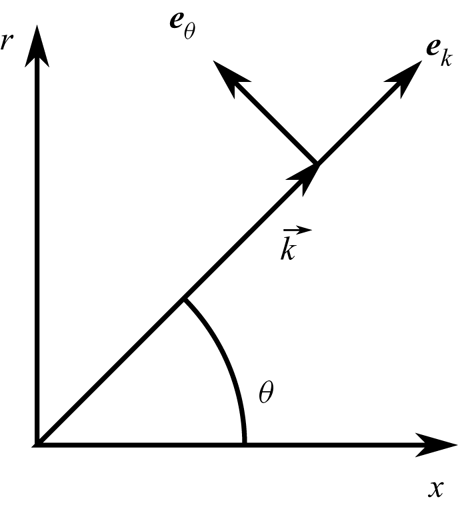
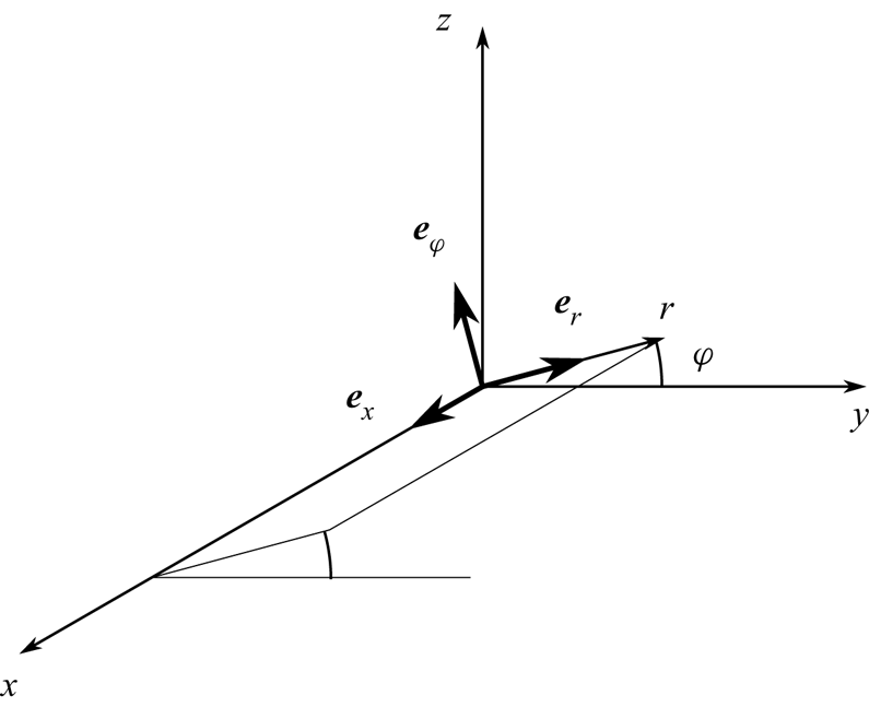
Single-wave LIA results are derived in a two-dimensional coordinate system (figure 2) and must be transferred to three dimensions for the study of isotropic disturbance fields. Define a three-dimensional Cartesian coordinate system  $(x,y,z)$ and a cylindrical coordinate system
 $(r,\varphi ,x)$ that share a common
 $x$ axis which points in the mean flow direction. See figure 3. The azimuthal angle
 $\varphi$ measures the orientation of the unit vector
 $\boldsymbol {e}_r$ in the
 $yz$-plane (positive in the counterclockwise sense from the
 $+y$ direction), and the unit vector
 $\boldsymbol {e}_\varphi$ is oriented such that
 $\boldsymbol {e}_{\varphi }=\boldsymbol {e}_{x}\times \boldsymbol {e}_{r}$. The
 $y$ and
 $z$ coordinates are related to
 $r$ and
 $\varphi$ by
 \begin{gather} y=r\cos\varphi, \end{gather}
 \begin{gather} z=r\sin\varphi . \end{gather}
The azimuthal angle  $\varphi$ is selected such that the wave vector
 $\boldsymbol {k}$ of the elementary wave under consideration lies in the
 $x$–
 $r$ plane. The wave vector makes an angle
 $\theta$ with the
 $x$-axis as in figure 2.
Two-dimensional coordinate system aligned with the wave vector.

Cylindrical coordinate system.

Since the solenoidal velocity field is composed solely of transverse waves whose velocity fluctuations are normal to their wave vectors (Moyal Reference Moyal1952), we have  ${\textrm {d}\boldsymbol {\hat {u}}({\boldsymbol {k}})\boldsymbol {\cdot }\boldsymbol {k}=0}$, and thus for isotropy, the energy associated with wave vector
 $\boldsymbol {k}$ is distributed equally between the two directions orthogonal to
 $\boldsymbol {k}$
 \begin{gather} {[} u'_k u'_k]_1^{vort.} = 0 \quad \text{(no summation)} \end{gather}
 \begin{gather}{[} u'_\theta u'_\theta]_1^{vort.}=[ u'_\varphi u'_\varphi ]_1^{vort.}=\dfrac12 [ u'_xu'_x+u'_yu'_y+u'_zu'_z]_1^{vort.}. \end{gather}
Note that, in (4.12), the subscripts  $k$,
 $\theta$ and
 $\varphi$ refer to coordinate directions and are not repeated indices to be summed over.
The out-of-plane part  $[u'_\varphi \, u'_\varphi ]_1^{vort.}$ contributes solely to the transverse spectra
 $[ u'_y\, u'_y+ u'_z\, u'_z]_1^{vort.}$. The in-plane part
 $[ u'_\theta \, u'_\theta ]_1^{vort.}$ contributes both to
 $[u'_x\, u'_x]_1^{vort.}$ and to
 $[u'_y\, u'_y+ u'_z\, u'_z]_1^{vort.}$.
For vortical waves, trigonometry leads to
 \begin{gather} u_x'^{vort.}(\boldsymbol{x},t)=-\int \exp\left({\textrm{i}(\boldsymbol{k}\boldsymbol{\cdot}\boldsymbol{x}-\omega t)}\right) \sin(\theta)\, \textrm{d}\hat{u}^{in}(\boldsymbol{k}). \end{gather}
 \begin{gather} u_y'^{vort.}(\boldsymbol{x},t)=\int \exp\left({\textrm{i}(\boldsymbol{k}\boldsymbol{\cdot}\boldsymbol{x}-\omega t)}\right) \cos(\theta)\,\cos(\phi)\, \textrm{d}\hat{u}^{in}(\boldsymbol{k})\nonumber\\ +\int \exp\left({\textrm{i}(\boldsymbol{k}\boldsymbol{\cdot}\boldsymbol{x}-\omega t)}\right) \sin(\phi)\, \textrm{d}\hat{u}^{out}(\boldsymbol{k}) \end{gather}
 \begin{gather} u_z'^{vort.}(\boldsymbol{x},t)=\int \exp\left({\textrm{i}(\boldsymbol{k}\boldsymbol{\cdot}\boldsymbol{x}-\omega t)}\right) \cos(\theta)\,\sin(\phi)\, \textrm{d}\hat{u}^{in}(\boldsymbol{k})\nonumber\\ \ +\int \exp\left({\textrm{i}(\boldsymbol{k}\boldsymbol{\cdot}\boldsymbol{x}-\omega t)}\right) \cos(\phi)\, \textrm{d}\hat{u}^{out}(\boldsymbol{k}), \end{gather}
where, for a given wave vector  $\boldsymbol {k}$,
 $\textrm {d}\hat {u}^{in}(\boldsymbol {k})$ and
 $\textrm {d}\hat {u}^{out}(\boldsymbol {k})$ are the contributions in and out of (normal to) the
 $x$–
 $r$ plane.
The overall procedure then for modelling the interaction of turbulence with a shock wave under linear theory is to compute an incident spectrum from (4.9), apply the single-wave LIA results to each elementary Fourier wave and then sum the resulting post-shock waves.
The in-plane part  $\textrm {d}\hat {u}^{in}$ of the incident turbulence is amplified according to a transfer function
 $G(\theta _1^{vort.},M_1,\gamma )$ which is computed as part of the LIA solution. The transfer function depends on in incidence angle
 $\theta _1^{vort.}$, on the incident Mach number
 $M_1$ and on the specific heat ratio
 $\gamma$. The out-of-plane part
 $\textrm {d}\hat {u}^{out}$ of the incident turbulence involves velocity fluctuations parallel to the shock and therefore passes through with constant amplitude. Thus the emitted amplitude spectra (subscript 2) are related to the incident spectra by
 \begin{gather} \textrm{d}\hat{u}_2^{in}(\boldsymbol{k}_2^{vort.}) =G \textrm{d}\hat{u}_1^{in} (\boldsymbol{k}_1^{vort.}), \end{gather}
 \begin{gather} \textrm{d}\hat{u}_2^{out}(\boldsymbol{k}_2^{vort.})=\textrm{d}\hat{u}_1^{out}(\boldsymbol{k}_1^{vort.}), \end{gather}
where the wave vector  $\boldsymbol {k}_2^{vort.}$ of the emitted wave is related to the wave vector
 $\boldsymbol {k}_1^{vort.}$ of the incident wave by a refraction law.
From (4.13) and (4.14) it follows that, according to LIA, the immediate post-shock spectra due solely to the vortical fields are related to the incident spectra by
 \begin{gather} \begin{gathered}{[u'_{x}u'_{x}]}^{vort.}_{2} = \sin^2(\theta_{2})\vert G\vert^{2} [u'_{\theta} u'_{\theta}]_{1} = \sin^2(\theta_{2})\vert G\vert^{2} \frac{1}{2} [u'_{j} u'_{j}]_{1},\nonumber\\ [u'_{y}u'_{y}]^{vort.}_{2}+ [u'_{z} u'_{z}]^{vort.}_{2} = [u'_{\phi} u'_{\phi}]_{1}+\cos^2(\theta_2)\vert G \vert^2 [u'_{\theta} u'_{\theta}]_{1}\end{gathered}\end{gather}
 \begin{gather}= (1+\cos^2(\theta_2)\vert G\vert^2) \frac12 [u'_j u'_j]_1, \end{gather}
where summation is to be applied over the index  $j$.
4.4. Post-shock evolution of vortical modes
We consider the streamwise evolution of each vortical mode individually. As a vortical wave convects downstream, some of its energy is dissipated by viscosity and some is redistributed by nonlinear effects to other modes in a more ‘scrambled’ state about which less is known. The former is straight forward to compute directly, but the latter is modelled here in terms of an eddy viscosity. Despite the approach of considering each Fourier mode individually, the eddy viscosity preserves the basic nonlinearity of the governing equations and creates an interdependence between each mode and the overall TKE at a given streamwise station.
Recall from § 4.1 that the LIA-predicted amplitude differentials such as the generic  $\textrm {d}\hat {a}'(\boldsymbol {k})$ and
 $\textrm {d}\hat {b}'(\boldsymbol {k})$ and the associated correlation spectrum
 $[a'b']$ are independent of
 $x$ under the definitions used here. Now we seek to include both viscous effects and an eddy viscosity model for the nonlinear interactions between Fourier modes. These effects lead to a departure from the inviscid LIA solution and hence introduce a dependence of the spectra on
 $x$. We use the subscript LIA to denote what remains of the LIA-predicted amplitude in a given Fourier mode at a certain streamwise location. For example, we write the remaining amplitude of a Fourier vortical wave as
 $\textrm {d}\hat {u}_{LIA}^{vort.}(\boldsymbol {k})$. At
 $x=0$, the values of all post-shock amplitudes and spectra match their LIA-predicted values. The effect of viscosity is to dissipate the vortical motions. For a post-shock elementary wave
 $\textrm {d}\hat {u}_{LIA}^{vort.}(\boldsymbol {k}_2^{vort.})$, the time rate of change in amplitude due to viscosity is
 $-\nu k^2 \textrm {d}\hat {u}_{LIA}^{vort.}(\boldsymbol {k})$. Similarly, the rate of change of the amplitude due to nonlinear effects is modelled by a turbulent diffusivity
 $\nu _t$ as
 $-\nu _t k^2 \textrm {d}\hat {u}_{LIA}^{vort.}(\boldsymbol {k})$. Both of these effects transfer energy out of the Fourier mode under consideration. In the case of viscosity, the energy is converted into thermal energy, whereas in the case of the turbulent viscosity, the energy is transferred to other turbulent motions and will be accounted for separately.
With the inclusion of molecular and eddy viscosity, the streamwise evolution (represented here by the  $x$-dependence of
 $\textrm {d}\hat {u}$) of one Fourier mode in the remnant of the LIA-predicted vortical field is governed by
 \begin{equation} \dfrac{\textrm{D}}{\textrm{D} t } \textrm{d}\hat{u}_{LIA}^{vort.}(\boldsymbol{k}) = U\dfrac{d}{{\textrm{d}x} } \textrm{d}\hat{u}_{LIA}^{vort.}(\boldsymbol{k}) = -\nu k^2 \textrm{d}\hat{u}_{LIA}^{vort.}(\boldsymbol{k}) - \nu_t k^2 \textrm{d}\hat{u}_{LIA}^{vort.}(\boldsymbol{k}), \end{equation}
where  $\textrm {D}/\textrm {D}t$ is a Lagrangian time derivative based on the mean flow velocity. The eddy viscosity
 $\nu _t$ is defined by
 \begin{equation} \nu_t=C_\mu f_\mu \sqrt{\frac12 R_{jj}} \ell_{LIA}, \end{equation}
where  $C_\mu =0.09$ is a model parameter,
 $\ell _{LIA}$ is a length scale of the LIA-predicted post-shock turbulence and
 $f_\mu =\exp (-2.5/(1+Re_{T}/50))$ is a damping function due to Jones & Launder (Reference Jones and Launder1972) that is designed to account for low Reynolds number effects. Here,
 $Re_T=(\sqrt {R_{jj}/2}) \ell _{LIA}/\nu _2$.
To obtain a length scale representative of the LIA-predicted post-shock turbulence, we first compute a TKE-weighted average of the post-shock wavenumber according to
 \begin{equation} {k_{LIA}}=\dfrac{\int \dfrac12\, {k_2^{vort.}} (1+\vert G \vert^2) \,\textrm{d}\boldsymbol{k}_1^{vort.}}{\int \dfrac12 (1+\vert G \vert^2) \,\textrm{d}\boldsymbol{k}_1^{vort.}} \end{equation}
and then the length scale is defined as
 \begin{equation} \ell_{LIA} = 2{\rm \pi}/k_{LIA}. \end{equation}
The energy removed from the LIA-predicted field by molecular viscosity is simply converted into internal energy, but the energy removed by the eddy viscosity is transferred into other, primarily smaller, turbulent motions. This disordered or ‘scrambled’ TKE is represented in the model by two bins: one for streamwise velocity fluctuations, and one for transverse. Let us refer to the Reynolds stresses associated with the nonlinearly transferred TKE as  $R^{NL}_{\alpha \alpha }$ and those associated with the remnants of the LIA-predicted field as
 $R^{LIA}_{\alpha \alpha }$.
A specific degree of anisotropy can be associated with the energy transferred away from the LIA modes based on the relative rates of decrease in  $R_{11}^{LIA}$ and
 $R_{22}^{LIA}$. In this context anisotropy will be measured by the anisotropy tensor
 \begin{equation} a_{ij}\equiv\frac{R_{ij}}{R_{kk}}-\frac13\delta_{ij}. \end{equation}
Thus we represent the anisotropies of the energies drained by the eddy viscosity term from the LIA-predicted field (denoted  $\rm LIA\!\rightarrow$) and added to the nonlinearly transferred (NL) field (denoted
 $\rightarrow \textrm {NL}$) using the anisotropy tensors
 \begin{equation} a^{LIA\rightarrow}_{\alpha\alpha} \equiv \left.{\left[-{\dfrac{\textrm{D}}{\textrm{D}t}R_{\alpha\alpha}^{LIA}}\right]_{\nu_t}}\right/{\left[-{\dfrac{\textrm{D}}{\textrm{D}t}R_{kk}^{LIA}}\right]_{\nu_t}}-\frac13 \end{equation}
and
 \begin{equation} a^{\rightarrow {\rm NL}}_{\alpha\alpha} \equiv \left. {\left[{\dfrac{\textrm{D}}{\textrm{D}t}R_{\alpha\alpha}^{NL}}\right]_{\nu_t}}\right/{\left[{\dfrac{\textrm{D}}{\textrm{D}t}R_{kk}^{NL}}\right]_{\nu_t}}-\frac{1}{3}. \end{equation}
Here,  $[\cdot ]_{\nu _t}$ selects only the part of the rate of change that is due to the eddy viscosity. The quantity
 $a^{LIA\rightarrow }_{\alpha \alpha }$ depends on how strongly the eddy viscosity acts on each mode and is different from the overall anisotropy of the LIA-predicted field.
Tennekes & Lumley (Reference Tennekes and Lumley1972) (in their §§ 8.2 and 8.4) introduce a model for the energy cascade in homogeneous turbulence based on dividing the spectrum into discrete eddy sizes. They assume the degree of anisotropy inherited by eddies of a certain size from larger ones is proportional to the ratio of the time scale of the energy-recipient eddies over the time scale of the energy-donor ones. In the inertial subrange at least, this leads to the smaller eddies having approximately one half the anisotropy of the larger ones. While acknowledging the crude nature of this model, we adopt this assumption and partition the energy between  $R^{NL}_{11}$ and
 $R^{NL}_{22}$ such that the energy added to the NL bins retains half the anisotropy of the energy drained from the LIA-predicted modes. That is, we assume that
 \begin{equation} a^{\rightarrow\rm NL}_{\alpha\alpha} = \frac12 a^{\textrm{LIA}\rightarrow}_{\alpha\alpha}. \end{equation}
Furthermore, energy conservation requires that
 \begin{equation} \left[{\dfrac{\textrm{D}}{\textrm{D}t}R_{kk}^{NL}}\right]_{\nu_t} = -\left[{\dfrac{\textrm{D}}{\textrm{D}t}R_{kk}^{LIA}}\right]_{\nu_t}, \end{equation}
and axisymmetry requires that
 \begin{equation} R_{22}=R_{33} . \end{equation}
Equations (4.23) through (4.25) uniquely specify  $[{({\textrm {D}}/{\textrm {D}t})R_{\alpha \alpha }^{NL}}]_{\nu _t}$ in terms of the
 $[{({\textrm {D}}/{\textrm {D}t})R_{\alpha \alpha }^{LIA}}]_{\nu _t}$ computed from (4.17).
The viscous decay of the turbulence in the scrambled bins is modelled by a dissipation rate
 \begin{equation} \epsilon = A_\epsilon\left. \left(\frac{1}{3} R_{kk}^{NL}\right)^{3/2}\right/\ell_{NL}, \end{equation}
where  $A_\epsilon$ is a coefficient. In the case of grid turbulence, the experiments of Sreenivasan (Reference Sreenivasan1984) suggest
 $A_\epsilon \approx 0.5\text {--}0.75$ if we associate the longitudinal integral scale of the experiment with the length scale
 $\ell ^{NL}$. We choose
 $\ell _{NL}=0.38\ell _{LIA}$, which is motivated by the eddy size discretization in the model of Tennekes & Lumley (Reference Tennekes and Lumley1972). In Sreenivasan (Reference Sreenivasan1984), the value of
 $A_\epsilon$ rises at low Reynolds numbers; the Reynolds numbers considered here are toward the lower limit of the regime where
 $A_\epsilon$ is approximately constant. The dissipation is applied to
 $R_{11}^{NL}$ and
 $R_{22}^{NL}$ in proportion to their relative magnitudes so that the dissipation does not alter the anisotropy of the scrambled TKE. The dissipation rate defined here applies to TKE; the time rate of change of
 $R_{jj}^{NL}$ due to dissipation is therefore
 $2\epsilon$.
In the absence of an applied strain rate, the turbulence in the scrambled bins might be expected to return to isotropy. The simplest successful model for the return-to-isotropy effect in the absence of mean strain is a linear relation due to Rotta (Reference Rotta1951). When applied to the scrambled bins it becomes
 \begin{equation} \dfrac{\textrm{D}R^{NL}_{ij}}{\textrm{D}t} \approx - \dfrac{C_1}{\tau}\left(R^{NL}_{ij}-\dfrac13 R^{NL}_{kk} \,\delta_{ij}\right), \end{equation}
where  $\tau =(1/2) R_{kk}^{NL}/\epsilon$ is a time scale of the turbulence based on its most energetic scales (which in most cases are the scales at which the anisotropy resides) and
 $C_1$ is a closure coefficient for which the experiments of Uberoi (Reference Uberoi1956) imply a value in the neighbourhood of 1.4–1.8 (Wilcox Reference Wilcox1998). Rotta's model is further roughly confirmed by the measurements of Champagne, Harris & Corrsin (Reference Champagne, Harris and Corrsin1970) who find the constant to be 1.4, 1.3 or 2.0 depending on the Reynolds stress component being considered. Thus the rate of return of the scrambled TKE toward isotropy is approximately proportional to the anisotropy and inversely proportional to the turbulence time scale.
Here Rotta's model is applied only to the scrambled bins, not to the LIA-predicted field. From (4.26) the time scale can be written
 \begin{equation} \tau \approx 2.6 \ell_{NL} / A_\epsilon \sqrt{R_{kk}^{NL}}. \end{equation}
Any choice of fixed length scale based on  $L$ (as is the case with
 $\ell _{NL}$) becomes problematic farther downstream when the LIA field is essentially depleted of energy and becomes irrelevant. However, we mainly seek to understand the rapid adjustment of anisotropy closer to the shock.
4.5. Post-shock dilatational modes
The foregoing discussion specifies the modelled evolution of the vortical part of the post-shock solution; however, the shock–turbulence interaction also produces pressure fluctuations on the post-shock side. In addition to the transfer function  $G$, the LIA solution includes another dimensionless transfer function (call it
 $H$) that relates the post-shock pressure fluctuations to the incident vortical ones
 \begin{equation} \frac{\textrm{d}\hat{p}_2(\boldsymbol{k}_2^{ac.})}{P_2} =H \frac{\textrm{d}\hat{u}_1^{in} (\boldsymbol{k}_1^{vort.})}{U_{1}}. \end{equation}
Note that only the in-plane part of the vortical field produces post-shock pressure disturbances and that the wave vector  $\boldsymbol {k}_2^{ac.}$ of the emitted acoustic wave is distinct from that of the co-emitted vortical wave (
 $\boldsymbol {k}_2^{vort.}$). Depending on the incidence angle
 $\theta _1^{vort.}$, the pressure disturbance may be a propagating sound wave or an evanescent wave. In either case the associated dilatational velocity fluctuation may be written
 \begin{gather} \textrm{d}\hat{u}'^{ac.}_{2x}(\boldsymbol{k}^{ac.}_2) = \left(\cos(\theta^{ac.}_2)+\textrm{i}\eta\right) \exp\left({-\eta {k}^{ac.}_{2} x}\right) \frac{c_2 f_p}{\gamma U_1} H\, \textrm{d}\hat{u}'^{in}(\boldsymbol{k}^{vort.}_1), \end{gather}
 \begin{gather}\textrm{d}\hat{u}'^{ac.}_{2r}(\boldsymbol{k}^{ac.}_2) = \sin(\theta^{ac.}_2)\frac{c_2 f_p}{\gamma U_1} H\, \textrm{d}\hat{u}'^{in}(\boldsymbol{k}^{vort.}_1), \end{gather}
 \begin{gather}\textrm{d}\hat{u}'^{ac.}_{2\varphi}(\boldsymbol{k}^{ac.}_2) = 0, \end{gather}
where  $c_2$ is the post-shock speed of sound and
 $f_p$ is a dimensionless quantity that takes on a complex value for an evanescent pressure disturbance and a value of
 ${\pm }1$ for a propagating wave. The real-valued quantity
 $\eta$ represents the streamwise inviscid decay of an evanescent wave. Both
 $f_p$ and
 $\eta$ are obtained as part of the LIA solution. In the case of a propagating acoustic wave,
 $\eta =0$.
In isotropic turbulence, the dilatational motions are only weakly coupled with the vortical motions (Kida & Orszag Reference Kida and Orszag1990). We assume that the same is approximately true here; we include the dilatational modes in order to incorporate their contribution to the Reynolds stress, but they are assumed to evolve according to inviscid linear theory (i.e. they are not acted on by eddy viscosity or molecular viscosity).
The overall Reynolds stresses due to the combined vortical and acoustic parts of the LIA-predicted velocity fields may be written
 \begin{gather} (R_{11})_2^{LIA} = \left\{ (\overline{u'_xu'_x})_2^{vort.} + 2(\overline{u'^{vort.}_xu'^{ac.}_x})_2 + (\overline{u'_xu'_x})_2^{ac.} \right\}^{LIA}, \end{gather}
 \begin{gather}(R_{22})_2^{LIA} = \left\{ (\overline{u'_y u'_y})_2^{vort.} + 2(\overline{u'^{vort.}_y u'^{ac.}_y})_2 + (\overline{u'_y u'_y})_2^{ac.}\right\}^{LIA}. \end{gather}
Correlations and cross-correlations appearing in (4.31) such as  $(\overline{u'^{vort.}_xu'^{ac.}_x})_2^{LIA}$ are computed by substituting (4.30) and the local value of
 $\textrm {d}\hat {u}^{vort.}_{LIA}$ (which includes modifications due to viscous and nonlinear effects) along with appropriate trigonometric functions into (4.4) and (4.5).
For example we have
 \begin{align} (\overline{u'^{vort.}_xu'^{ac.}_x})_2^{LIA}&=\int \exp \left(i(k_{2x}^{ac.}-k_{2x}^{vort.\ast})x\right) \left[u'^{vort.}_{2x}u'^{ac.}_{2x}\right]^{LIA} \textrm{d}\boldsymbol{k}_2 \nonumber\\ &=\int \exp\left(i(k_{2x}^{ac.}-k_{2x}^{vort.\ast})x\right) \overline{\textrm{d}\hat{u}'^{vort. \ast}_{2x} \left(\boldsymbol{k}^{vort.}_2\right) \textrm{d}\hat{u}'^{ac.}_{2x} \left(\boldsymbol{k}^{ac.}_2\right)}, \end{align}
where
 \begin{equation} \textrm{d}\hat{u}'^{vort. \ast}_{2x}\left(\boldsymbol{k}^{vort.}_2\right)=- \sin\left(\theta_2^{vort.}\right)\, \textrm{d}\hat{u}'^{vort. \ast}_{LIA}\left(\boldsymbol{k}^{vort.}_2\right) \end{equation}
and  $\textrm {d}\hat {u}'^{ac.}_{2x}\left (\boldsymbol {k}^{ac.}_2\right )$ is given by (4.30a).
In the immediate post-shock region, the fluctuating pressure field is dominated by contributions from evanescent waves. These waves are associated with significant dilatational velocity fluctuations that partially cancel the vortical velocity fluctuations, and their inviscid decay causes a rapid post-shock increase in TKE as observed in DNS.
There is little exchange of TKE between the acoustic and vortical modes in the post-shock region, as is evident from the fact that DNS post-shock TKE results extrapolated back to the mean shock location agree quite well with LIA predictions based solely on the emitted vortical field. (In other words, as soon as it is emitted from the shock, the vortical field already contains sufficient energy to account for the TKE observed farther downstream.) Thus, although the evanescent pressure fluctuations are quite strong and directly affect the Reynolds stress profiles in the immediate post-shock region, they do not have much lasting impact on the TKE of the vortical field, which dominates beyond approximately  $x=L/2$ and which is of primary interest here.
This line of reasoning contradicts some statements in the literature regarding the role of the post-shock dilatational field, and especially of the evanescent part of it. It is apparently not true that the dilatational modes give up their energy to the vortical modes to account for the rapid increase in TKE behind the shock. In order for that picture to be correct, energy imparted to the dilatational waves at the shock would need to be transported by the dilatational waves away from the shock and gradually transferred to the vortical modes. In reality this required streamwise energy flux is absent from the evanescent waves that dominate the dilatational field. As the angle of incidence for a vortical wave approaches the critical angle where the post-shock pressure disturbance becomes evanescent, the energy flux vector of the acoustic wave becomes oriented parallel to the shock. When the incidence angle reaches the evanescent regime, streamwise energy transport by the pressure disturbance ceases. This can be seen by considering an isolated evanescent wave. It is a valid solution to the (linearized) post-shock governing equations and decays with streamwise distance. Its decay does not produce any vortical wave. There is no fluctuation energy whatsoever in the limit  $x\rightarrow \infty$, and therefore, since the solution is periodic in time and not exponentially growing, there cannot have been any energy carried away from the shock by the evanescent wave. Once the periodic solution has somehow been established (in reality, this would correspond to some transient period), the evanescent field does contain energy, but it retains it for all time. The situation is different for acoustic waves in the propagating regime. They do have a small associated streamwise energy flux, but under LIA theory they propagate without attenuation and therefore also cannot be the source of any increased TKE in LIA solutions. Lee et al. (Reference Lee, Lele and Moin1993) claimed that the increase in TKE was made possible by a transfer of energy from the mean, not fluctuating field. The present model is in harmony with this view.
4.6. Effect of shock motion
The final consideration in developing the model is that the motion of the shock wave leads to large streamwise velocity fluctuations near the mean shock location. LIA solutions can provide a root-mean-square shock excursion distance, and this, combined with the mean Rankine–Hugoniot jumps is enough information to approximate the variance due to shock motion. Under LIA theory, the shock motion is caused by the integrated effects of infinitesimal incident Fourier modes, and these modes are pairwise independent. The central limit theorem may be applied to show that the leading-order part of the shock motion follows a normal distribution. This implies a sigmoidal shape for the mean velocity profile based on the cumulative density function (CDF) of a normal random variable. Larsson et al. (Reference Larsson, Bermejo-Moreno and Lele2013) show how knowledge of the mean profile and the Rankine–Hugoniot jumps can be used to yield the leading-order part of the shock-motion-induced peak in  $R_{11}$.
Let us refer to this contribution due to shock motion as  $R_{11}^{SM}$. Then the overall Reynolds stresses are built up as the sums
 \begin{gather} R_{11} = R_{11}^{LIA} + R_{11}^{NL} + R_{11}^{SM}, \end{gather}
 \begin{gather}R_{11} = R_{22}^{LIA} + R_{22}^{NL}. \end{gather}
More details on the computation of  $R_{11}^{SM}$ are provided in appendix A. In the cases considered here, the peak in
 $R_{11}$ due to shock motion is too narrow to be seen clearly in the figures; however, the tail of the peak helps to give the correct profile shape near to the shock.
5. Results and discussion
The anisotropy model produces streamwise profiles of Reynolds stresses. These may be divided roughly into three different types. Figure 4 presents a typical case from each type. The case at Mach 1.05 (figure 4a) features relatively fast development of a quasi-steady TKE level. This is due to the rapid inviscid decay of evanescent waves in cases at low Mach numbers. The oscillations are a consequence of choosing a monochromatic spectrum; a more realistic spectrum would smooth out these oscillations. The Mach 1.5 case (figure 4b) features the rapid post-shock rise in TKE that is familiar in the literature for most SITI cases. For this case, inviscid LIA would predict a constant anisotropy value with  $R_{11}>R_{22}$ beyond some streamwise location, and thus there would be qualitative agreement between LIA and DNS. The model modifies the LIA-predicted anisotropy only moderately in this case. In the Mach 3.5 case (figure 4c), however, inviscid LIA predicts
 $R_{22}>R_{11}$, whereas the model produces both a significant increase in
 $b\equiv R_{11}/R_{22}$ closely following the shock and then a slower rise farther downstream.
Post-shock evolution of Reynolds stresses and anisotropy  $R_{11}/R_{22}$ as predicted by the present model for: (a)
 $M=1.05$,
 $M_t=0.05$,
 $Re_L=180$; (b)
 $M=1.5$,
 $M_t=0.15$,
 $Re_L=180$; and (c)
 $M=3.50$,
 $M_t=0.16$,
 $Re_L=200$.

Larsson et al. (Reference Larsson, Bermejo-Moreno and Lele2013) report Reynolds stress and anisotropy ratio profiles for DNS cases with  $M=3.50$,
 $M_t=0.15\text {--}0.16$, and
 $Re_L=200$ and
 $670$. Figure 5 compares the present model profile with their data. The model curves are qualitatively similar to the DNS, with the majority of the anisotropy discrepancy (with respect to LIA) appearing within about
 $L/2$ of the shock and then with a subsequent further gradual increase. In these two cases, the model accounts for three quarters or more of the anisotropy ratio discrepancy between the LIA predictions and the DNS profiles.
Comparison of post-shock Reynolds stress anisotropy ratio  $R_{11}/R_{22}$ for
 $(M,M_t)=(3.50,0.15\text {--}0.16)$: DNS of Larsson et al. (Reference Larsson, Bermejo-Moreno and Lele2013) (
 $Re_L=200$ – solid,
 $Re_L=670$ – short dash); present model (
 $Re_L=200$ – long dash,
 $Re_L=670$ – dash-dot-dot). LIA from Sinha, Mahesh & Candler (Reference Sinha, Mahesh and Candler2003) (dash-dot) and experimental results of Barre et al. (Reference Barre, Alem and Bonnet1996) (crosses) are also plotted. Reproduced from Larsson et al. (Reference Larsson, Bermejo-Moreno and Lele2013) with data added.

In order to compare many sets of flow parameters between DNS and the model, it is helpful to distil each profile into a single anisotropy value as in Larsson et al. (Reference Larsson, Bermejo-Moreno and Lele2013). In the Mach 1.05 case, it seems reasonable to select a value in the middle of the oscillations. For the Mach 1.5 case and similar profiles, we select the local maximum anisotropy value in the vicinity of  $x=L$. In cases like the Mach 3.5 case, there is no local maximum of the anisotropy. It seems reasonable then to select the value at some streamwise station where the anisotropy has had enough chance to develop so that the change with distance is slow but also where there is still significant vortical TKE left. We choose
 $x/L = 4$.
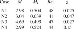
Figures 6(a) and 6(b), respectively, plot the post-shock anisotropy computed by DNS (Larsson et al. Reference Larsson, Bermejo-Moreno and Lele2013) and predicted by the proposed model for the flow parameters of Larsson et al. (Reference Larsson, Bermejo-Moreno and Lele2013) (table 1). DNS data at higher dilatational energy fraction  $\chi$ from Grube & Martín (Reference Grube and Martín2021) are included for comparison. (See parameters for cases N1–N4 in table 2.) The dilatational energy fraction increases from case N1 to N2 and again from N2 to N4. Note that the increasing dilatational energy in the incoming flow leads to significantly greater anisotropy levels. The present model only accounts for incident vortical fields (i.e. incompressible turbulence), and so it is not applicable to cases such as those in Grube & Martín (Reference Grube and Martín2021). The DNS cases of Larsson et al. (Reference Larsson, Bermejo-Moreno and Lele2013) are essentially incompressible and so a meaningful comparison can be made. Tables 1 and 2 list the flow conditions.
Post-shock Reynolds stress anisotropy ratio  $R_{11}/R_{22}$ for the cases of Larsson et al. (Reference Larsson, Bermejo-Moreno and Lele2013) as computed by (a) DNS and (b) the proposed anisotropy model. DNS data at higher dilatational energy fractions
 $\chi$ from cases N1–N4 of Grube & Martín (Reference Grube and Martín2021) are also plotted for comparison. The proposed model considers only vortical turbulence impinging on the shock, and so the model is not applicable to the cases N1–N4. For the cases of Larsson et al. (Reference Larsson, Bermejo-Moreno and Lele2013), different
 $M_t$ values at a given
 $M$ are indicated (in order of increasing
 $M_t$) by circles, squares, diamonds and triangles for
 $Re_l\approx 200$ and plus, cross and star for
 $Re_L\approx 660$. The N-series DNS data are plotted using filled circles and are individually labelled. Tables 1 and 2 list the flow conditions. Note that, in the data points of Larsson et al., a symbol may be shared by two data points that do not share a common
 $M_t$. The LIA prediction is shown as a solid curve.

Pre-shock flow parameters from the DNS cases of Larsson et al. (Reference Larsson, Bermejo-Moreno and Lele2013).

Pre-shock flow parameters from the N-series DNS cases of Grube & Martín (Reference Grube and Martín2021). Here  $\chi \equiv$ dilatational TKE/total TKE.

In order to avoid overfitting, the model has been computed using standard parameter values from the literature. We choose  $A_\epsilon =0.5$ based on Sreenivasan (Reference Sreenivasan1984),
 $C_1=1.6$ which is the middle of the range suggested by Wilcox (Reference Wilcox1998), and
 $C_\mu =0.09$ which is the standard value for
 $k$–
 $\epsilon$ models such as Launder & Sharma (Reference Launder and Sharma1974). No attempt has been made to tune the parameters.
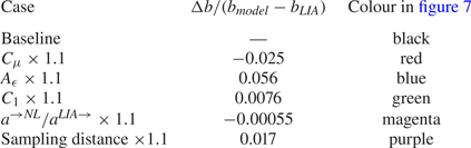
The sensitivity of the anisotropy to the model parameters is investigated by increasing each parameter by 10 % one at a time and plotting the resulting anisotropy values using different colours in figure 7. The Mach 4.7 data point is representative of the high Mach number cases; let us examine that case in detail. Table 3 lists the change in model anisotropy at Mach 4.7 (normalized by the deviation of the baseline model from LIA) for a 10 % increase in various model parameters. As above, the baseline model uses  $C_\mu =0.09$,
 $A_\epsilon =0.5$ and
 $C_1=1.6$. In addition, half the anisotropy of the energy lost by the LIA field is retained as the energy is added into the NL bins (
 $a^{\rightarrow NL}/a^{LIA\rightarrow }=0.5$), and the representative value of the anisotropy ratio is taken to be the maximum up to
 $x/L=4$ (excluding the shock-motion-induced peak). A 10 % increase in any of these parameters leads to a smaller relative change in the anisotropy. The anisotropy is most sensitive to
 $A_\epsilon$ where the 10 % increase results in a 5.6 % increase in normalized anisotropy. The next most sensitive parameter is
 $C_\mu$, where a 10 % increase results in a 2.5 % decrease in normalized anisotropy. The model is remarkably insensitive to the fraction of anisotropy retained by the energy as it is transferred from the LIA field to the NL bins, where a 10 % increase gives a decrease in normalized anisotropy of just six parts in ten thousand. This is fortunate since the model in Tennekes & Lumley (Reference Tennekes and Lumley1972) is rather crude and this fraction of inherited anisotropy has not been calibrated in the same way that other model coefficients have been.
Model anisotropy for the cases of Larsson et al. (Reference Larsson, Bermejo-Moreno and Lele2013) computed with various model parameters increased by 10 %. Symbols are as in figure 6. See table 3 for explanation of colours.

Sensitivity of the anisotropy at Mach 4.7 to 10 % increments in model parameters.

In comparing figures 6(a) and 6(b), we see that the model has relatively little effect at low supersonic Mach numbers where the LIA prediction is already fairly accurate. By approximately Mach 1.5, both the model and the DNS depart from the LIA predictions, with the model lagging a bit. As the Mach number increases, so does the wave front compression that the model is motivated by. Beyond about Mach 2, the LIA prediction calls for an anisotropy less than unity, whereas both the DNS and model predict roughly constant anisotropy values of approximately 1.2 to 1.3 for the model and 1.3 to 1.4 for the DNS. Considering that the LIA prediction is much less than unity, a discrepancy of 0.1 between the model and DNS is small compared to the difference between LIA and the model or DNS results. The model's behaviour as a function of Mach number is an improvement over LIA theory alone, but the behaviour as a function of  $M_t$ is less clear. In the DNS, it appears that the anisotropy is a weak function of
 $M_t$ and that as
 $M_t$ rises, so does the anisotropy, especially for the highest fluctuation cases where the shock enters the broken regime. However, this seems to be true only below Mach 2. At Mach 3.5 the DNS shows very little dependence on
 $M_t$. Below about Mach 2 it appears that increasing
 $M_t$ causes the model to predict lower anisotropy, which is opposite to the DNS trend. Above Mach 2 the opposite is true.
The model and DNS results also depend on Reynolds number. At high Mach numbers, a higher  $Re$ leads to a lower anisotropy. This may be due to the fact that
 $R_{22}$, which consists of spatially compressed modes is acted on more strongly than
 $R_{11}$ by both the molecular viscosity and the eddy viscosity. When a given amount of energy is removed from
 $R_{22}$ by the eddy viscosity, it is not removed from the total TKE flow, but rather it is moved toward local isotropy as it is added into the scrambled turbulence bins of the model. On the other hand, energy removed from
 $R_{22}$ by the action of molecular viscosity is removed from the overall TKE. Thus molecular viscosity drives the anisotropy toward some larger positive value, whereas the eddy viscosity drives it locally toward unity. We expect then that the greater action of molecular viscosity at lower Reynolds numbers should lead to higher anisotropy values, as is observed both in the DNS and in the model predictions at Mach 3.5.
As with the  $M_t$ dependence, the
 $Re$ dependence is qualitatively reversed below about Mach 2. This may indicate that there is some other physical mechanism besides the wave front compression that is important at these lower Mach numbers. However, the model and DNS curves are already relatively close to the LIA curve in this region. The success of the model at higher Mach numbers indicates that, at least where the compression is strong, the departure from the LIA-predicted anisotropy can be explained as a result of the strong local anisotropy imparted to the turbulence upon passage through the shock.
6. Summary
The discrepancy in post-shock Reynolds stress anisotropy between LIA predictions and DNS data is a longstanding question. Since DNS makes no modelling assumptions pertaining to turbulence, it seems that the discrepancy must be a result of one or more of the assumptions or approximations made in the linear analysis. After assessing these assumptions, we argue that the post-shock nonlinear effects, which are missing in LIA, are the driving mechanism for the unexplained Reynolds stress evolution downstream of the shock.
An explanation is proposed as to how these nonlinear effects, which might be expected to promote isotropy in most situations, can in fact produce anisotropy in the post-shock region. Linear analysis shows that immediately downstream of the shock, the length scales of the vortical waves that contribute the majority of  $R_{22}$ are smaller than those that contribute the majority of
 $R_{11}$. In turn, the evolution of the motions that contribute the majority of
 $R_{22}$ occurs at a faster time scale. In essence, the energy in
 $R_{11}$ and
 $R_{22}$ is out of equilibrium behind the shock, with the energy in
 $R_{22}$ more quickly transferring away, allowing
 $R_{11}$ to prevail as both components decay and the flow ultimately returns toward equilibrium.
A quantitative model is presented which demonstrates the plausibility of the proposed explanation for the anisotropy. To represent the physics of the post-shock near-field non-equilibrium environment, we use an eddy viscosity to approximate the effects of nonlinear terms on individual Fourier wave modes. As energy is transferred away from these LIA-predicted modes by nonlinear effects, it is added to a collection of scrambled turbulence whose evolution is described by Rotta's return-to-isotropy model and viscous dissipation. The LIA–eddy viscosity hybrid model predicts post-shock Reynolds stress anisotropies close to those observed in DNS data for high Mach numbers and predicts, as in DNS, that the discrepancy with LIA vanishes for vanishingly weak shocks.
Funding
This work was supported in part by the Air Force Office of Scientific Research under award number FA 9550-17-1-0104 with Dr I. Leyva and the Air Force Testing and Evaluation Division under award number FA 9550-10-0535 with the Center for Testing Excellence at the University of Maryland and the Arnold Engineering Development Center with Mr D. Marren, Mr J. Lafferty and Dr E. Marineau.
Declaration of interests
The authors report no conflict of interest.
Appendix A. Shock-motion contribution to Reynolds stress profiles
Within the region of unsteady shock motion, the passage of the shock wave back and forth across a particular point causes the solution at that point to intermittently assume values close to the pre- and post-shock Rankine–Hugoniot states. This results in a very large contribution of  $R^{SM}_{11}$ to the streamwise Reynolds stress that is unrelated to the usual idea of the kinetic energy content of turbulent motions.
Larsson et al. (Reference Larsson, Bermejo-Moreno and Lele2013) provide an expression (without derivation) for the variance of a generic quantity due to the shock motion. They supply the mean profile by way of DNS. Let us derive the expression and supply the mean profile from LIA theory.
Assume a disturbance strength small enough that the shock surface locally maintains its identity as an effectively discontinuous change in flow properties. Consider a point near the unperturbed shock location ( $x=0$). The local shock excursions carry the shock across this point from time to time, and thus the local value of a generic quantity
 $a$ intermittently takes on values close to the pre- and post-shock Rankine–Hugoniot values
 $a^{RH}_1$ and
 $a^{RH}_2$, depending on whether the shock is instantaneously down- or upstream of the point, respectively. If the shock is upstream of the point a fraction
 $p$ of the time, then the Reynolds-averaged value at that
 $x$ location is approximately
 $p a^{RH}_2+(1-p) a^{RH}_1$. In terms of probability, the mean is
 \begin{equation} {\bar{a}}(x)\approx a^{RH}_1 + \left(a^{RH}_2-a^{RH}_1\right){P}\left( x'_{phys.} \leq x\right), \end{equation}
where  $x'_{phys.}(y,z,t)=\mathrm {Re} (x'_{s}(y,z,t))$ is the physical (real) part of the complex local shock displacement predicted by LIA.
Each elementary (Fourier) wave in the incident disturbance field causes a corresponding infinitesimal sinusoidal shock displacement. The complex shock displacement can be written as the Fourier–Stieltjes integral
 \begin{equation} x'_{s}= \int_{\boldsymbol{k}_1} \exp\left({\textrm{i}(k_y y+k_z z-\omega t)}\right) \dfrac{1}{k_1U_{1n}} G_{v\rightarrow x} \,\textrm{d}\hat{u}^{\prime \, vort.}(\boldsymbol{k}_1), \end{equation}
where  $G_{v\rightarrow x}$ is a non-dimensional transfer function between vortical velocity fluctuations and shock displacement that is obtained as part of the LIA solution. We are interested in the physical (real) part, so we define the root mean square shock displacement
 \begin{equation} x'_{rms}\equiv \sqrt{ \left\{\overline{\vphantom{M}x'_{s}x'_{s}}\right\}_{phys.} } = \sqrt{\frac{1}{2} \overline{\vphantom{M}x'_{s}x'_{s}} }. \end{equation}
Integrating (A2) in  $\boldsymbol {k}$-space over incidence angle
 $\theta _1$ and wavenumber magnitude
 $k_1$ leaves a dependence only on the azimuthal angle
 $\varphi _1$. Therefore
 $x'_{s}$ can be viewed as the sum of an infinite number of infinitesimally small real-valued random variables
 $\textrm {d}\hat {X}'(\varphi _1)$, each corresponding to the integrated contributions due to incident waves with a given azimuth
 $\varphi _1\in [0,2{\rm \pi} )$. Each random variable has zero mean, and the sum of their variances is the LIA-predicted variance. The spectrum function
 $\hat {u}^{\prime \, vort.}(\boldsymbol {k}_1)$ is in general discontinuous everywhere, and so the random variables
 ${\textrm {d}\hat {X}'(\varphi _1)}$ are independent of one another no matter how closely they are spaced in
 $\varphi _1$. Because of axisymmetry, all
 $\textrm {d}\hat {X}'(\varphi _1)$ are identically distributed. Furthermore, there are effectively infinitely many of them over the range
 $\varphi _1\in [0,2{\rm \pi} )$ since we can use as fine a partition as we wish in evaluating the integral. Therefore, we can be assured that no small collection of the random variables contributes an inordinate fraction of the total variance, and we are justified in applying the central limit theorem to the shock displacement, which is the sum of these infinitesimal random variables.
Let us partition  $[0,2{\rm \pi} )$ into
 $n$ equal segments
 $\Delta \varphi$, and let
 $\textrm {d}\hat {X}_i$ represent the contribution to the shock displacement from the segment containing
 $\varphi _i=\textrm {i}\Delta \varphi$. Because the total variance must match
 $\left \{\overline {x'_{s}x'_{s}}\right \}_{phys.}$, and because the
 $\textrm {d}\hat {X}_i$ are independent, we have
 \begin{gather} \left\langle \textrm{d}\hat{X}_i^{\prime} \textrm{d}\hat{X}'_i\right\rangle = \dfrac{\left\{\overline{x'_{s}x'_{s}}\right\}_{phys.}}{n} \quad (\text{no summation over }i), \end{gather}
 \begin{gather}\left\langle \textrm{d}\hat{X}_i^{\prime} \textrm{d}\hat{X}'_j\right\rangle=0 \quad i\ne j, \end{gather}
where  $\langle \cdot \rangle$ indicates an expectation value. Define
 \begin{equation} Y_n = \dfrac{\sum_{i=1}^n \textrm{d}\hat{X}'_i}{x'_{rms}}. \end{equation}
Then, upon re-normalization to account for the dependence of  $\textrm {Var}(\textrm {d}\hat {X}_i)$ on
 $n$ in the present case, the central limit theorem states that
 $Y_n$ converges in distribution to a standard normal random variable. As
 $n\rightarrow \infty$, the probability density function of
 $x'_{phys.}$ becomes
 \begin{equation} f_{x'_{phys.}}(x)=\dfrac{1}{\sqrt{2{\rm \pi}}\ {x'_{rms}}}\ \exp\left({-\dfrac{x^2}{2x_{rms}^{\prime 2}}}\right). \end{equation}
The corresponding cumulative distribution function (CDF) of  $x'_{phys.}$ is
 \begin{equation} F_{x'_{phys.}}(x) \equiv P\left(x'_{phys.}(y,z,t)\leq x\right) = \int_{-\infty}^x f_{x'_{phys.}}(\tilde{x}) \,\textrm{d}\tilde{x} = {\varPhi\left(\frac{x}{x'_{rms}}\right)}, \end{equation}
where the CDF  $\varPhi$ of the standard normal distribution is given by
 \begin{equation} \varPhi(\xi) \equiv \dfrac{1}{\sqrt{2{\rm \pi}}} \int_{-\infty}^\xi \textrm{e}^{-{s^2}/{2}} \, \textrm{d}s. \end{equation}
Returning to (A1), we now have an expression for the leading term of the mean profile  $A(x)$ of a generic quantity in the shock vicinity
 \begin{equation} \bar{a}(x)\approx a^{RH}_1 + \left(a^{RH}_2-a^{RH}_1\right){\varPhi\left(x/x'_{rms}\right)}. \end{equation}
The variance of  $a$ is defined by
 \begin{equation} \textrm{Var}(a)={E}\left( (a-\bar{a})^2 \right). \end{equation}
As before, let
 \begin{equation} p\equiv {P}\left(x'_{phys.}\leq x\right). \end{equation}
Then
 \begin{equation} a \approx \begin{cases} a^{RH}_1 & \text{with probability }1-p,\\ a^{RH}_2 & \text{with probability }p, \end{cases} \end{equation}
and
 \begin{equation} \bar{a}\approx a^{RH}_1 + (a^{RH}_2-a^{RH}_1)p. \end{equation}
It follows that
 \begin{equation} (a-\bar{a})^2 \approx \begin{cases} \left(a^{RH}_1-a^{RH}_2\right)^2p^2 & \text{with probability }1-p,\\ \left(a^{RH}_1-a^{RH}_2\right)^2(1-p)^2 & \text{with probability }p, \end{cases} \end{equation}
and therefore
 \begin{align} \textrm{Var}(a)&= {E}\left( (a-\bar{a})^2 \right) \nonumber\\ &\approx (1-p)\left(a^{RH}_1-a^{RH}_2\right)^2p^2 + p\left(a^{RH}_1-a^{RH}_2\right)^2(1-p)^2\nonumber\\ &=\left(a^{RH}_1-a^{RH}_2\right)^2p(1-p). \end{align}
Since  $p$ is already known theoretically from the CDF given above, we could stop here. However, we can also work in terms of the mean profile which allows the variance to be extracted either from (A10) or from DNS mean profiles as in Larsson et al.
 \begin{align} \textrm{Var}(a)&\approx\left(a^{RH}_1-a^{RH}_2\right)^2p(1-p) \nonumber\\ &= \left[ p\left(a^{RH}_1-a^{RH}_2\right)\right]\times \left[(p-1)\left(a^{RH}_2-a^{RH}_1\right)\right]\nonumber\\ &= \left(a^{RH}_1-\bar{a}\right) \left(\bar{a}-a^{RH}_2\right). \end{align}
The final line of (A17) is obtained by using (A14) to rewrite the bracketed quantities in terms of the Rankine–Hugoniot and mean states. From (A17), the maximum value of the variance due to the shock motion occurs when  $\bar {a}=(a^{RH}_1+a^{RH}_2)/2$ and is equal to
 $(a^{RH}_2-a^{RH}_1)^2/4$.
The smoothing of the mean profile resulting from (A10) is illustrated in figure 8 for a generic variable whose classical Rankine–Hugoniot value is assumed to jump from 1 to 10 across the shock. The variance as predicted by (A17) is also plotted. In this example, its maximum value is  $(10-1)^2/4=20(1/4)$.
Smoothing of the mean profile of a generic quantity due to shock motion. The pre- and post-shock Rankine–Hugoniot states are taken to be 1 and 10, respectively. The variance due solely to the shock motion is determined by the mean profile and is also shown.

Note that the derivation of (A17) began with the assumption of uniform states on either side of the shock. In reality the pre- and post-shock states are not perfectly constant and are not exactly given by the usual Rankine–Hugoniot normal shock relations. Therefore, there is some error involved in determining the variances from the means in this simplified manner. Nevertheless, the DNS study of Larsson et al. (Reference Larsson, Bermejo-Moreno and Lele2013) showed excellent agreement between the actual variance and that predicted by (A17), at least for their selected example case with relatively weak turbulence ( $M_t/M\approx 0.09$).
Applying this analysis to the streamwise velocity yields a leading-order estimate of the extra Reynolds stress  $R_{11}^{SM}$ as an effect of shock motion.