



1. Introduction
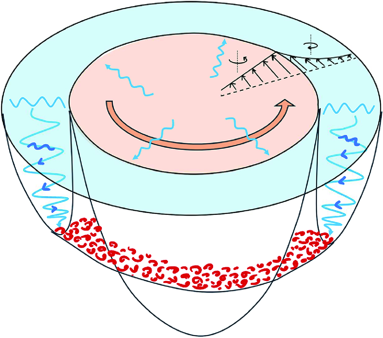
Near-inertial waves (NIWs) are disturbances to the balanced flow in the ocean, with frequencies close to the inertial frequency (
 $f = 2\Omega \sin \theta$
, where
 $\Omega$
is Earth’s rotation rate, and
 $\theta$
is the latitude), with large horizontal and small vertical wavelength, generated primarily by the wind stress (Alford et al. Reference Alford, MacKinnon, Simmons and Nash2016). Due to their large vertical shear, they play a dominant role in vertical mixing (Wunsch & Ferrari Reference Wunsch and Ferrari2004) and the oceanic energy budget (Munk & Wunsch Reference Munk and Wunsch1998). The NIWs can interact energetically with the balanced flows and can act, interestingly, as an energy source and an energy sink for the balanced flow under different conditions (see Gertz & Straub Reference Gertz and Straub2009; Whitt & Thomas Reference Whitt and Thomas2015; Taylor & Straub Reference Taylor and Straub2020; Thomas & Arun Reference Thomas and Arun2020; Thomas & Daniel Reference Thomas and Daniel2021). Factors such as
 $\beta$
-refraction (Gill Reference Gill1984) and mean flow vorticity (
 $\zeta$
-refraction; Asselin & Young 2020) can modify the propagation characteristics of NIWs, among others. In the latter case, the geostrophic mean flow vorticity (
 $\zeta$
) reduces the local NIW frequency, ‘trapping’ NIWs in the anticyclonic regions – i.e. regions of negative (positive)
 $\zeta$
in the northern (southern) hemisphere – leading to their downward propagation and subsequent dissipation at a critical depth (Lee & Niiler Reference Lee and Niiler1998). Over the years, numerous observational studies reported concentrated NIW energy in anticyclonic regions (Perkins Reference Perkins1976; Elipot, Lumpkin & Prieto Reference Elipot, Lumpkin and Prieto2010; Voet et al. Reference Voet2024), providing support for this theory. In the atmosphere, inertial-gravity waves are known to be generated from vortex dipoles and jets (Snyder et al. Reference Snyder, Muraki, Plougonven and Zhang2007; Wang, Zhang & Snyder Reference Wang, Zhang and Snyder2009) and can interact with the balanced flows (Serafimovich et al. Reference Serafimovich, Hoffmann, Peters and Lehmann2005; Niranjan Kumar et al. Reference Niranjan Kumar, Rao, Sandeep and Rao2014).
Kunze (Reference Kunze1985) showed NIW trapping using the Wentzel-Kramers-Brillouin-Jeffreys (WKBJ) approximation (i.e. the horizontal wavelengths of NIWs are considered to be smaller than the mean flow length scale) to derive the NIW dispersion relation. He showed that the lower bound of the NIW frequency band shifts to an effective Coriolis frequency given by
 $f_{e} = f\sqrt {1+Ro_{g}} \approx f + \zeta /2$
, where the approximation is valid for small-gradient Rossby numbers
 $Ro_g=\zeta /f$
. Here,
 $\zeta (x,z)$
is the relative vorticity, while
 $x$
and
 $z$
are horizontal and vertical coordinates of a front, respectively. Using a ray-tracing approach in a model of barotropic and baroclinic jets, he demonstrated trapping of NIWs with frequencies
 $f_e\lt \omega \lt f$
in negative vorticity regions. It should be noted that the horizontal length scales of initial wind-generated NIWs are typically an order of magnitude larger than the geostrophic mean flow length scales, contrary to the aforementioned WKBJ approximation. For such a scenario, Young & Ben Jelloul (Reference Young and Ben Jelloul1997) developed a theory using multiple-scale analysis for a narrow band of NIWs with frequencies close to the inertial frequency; improvements on the theory have been reported in the subsequent literature (Thomas, Smith & Bühler Reference Thomas, Smith and Bühler2017; Asselin & Young Reference Asselin and Young2019). However, the WKBJ theory still provides an easier alternative to the latter in understanding NIW dynamics, their vertical propagation through ray tracing, and especially the location of the critical layer. For this reason, WKBJ theory and ray tracing have been employed frequently in observational studies (Kunze, Schmitt & Toole Reference Kunze, Schmitt and Toole1995; Lelong, Cuypers & Bouruet-Aubertot Reference Lelong, Cuypers and Bouruet-Aubertot2020; Xu et al. Reference Xu, Zhao, Huang, Hu, Guan, Zhou and Tian2022). A recent study by Conn, Callies & Lawrence (Reference Conn, Callies and Lawrence2025) found that the WKBJ approach can be reconciled with the Young-Ben Jelloul (YBJ) method in the limit of weak-dispersiveness of NIW modes. Using a global plot of wave dispersiveness, they showed that high modes and high latitudes are weakly dispersive compared to low modes and mid/low latitudes, respectively (see for eg. Klein & Treguier Reference Klein and Treguier1994; Klein & Smith Reference Klein and Smith2001).
Recently, Whitt & Thomas (Reference Whitt and Thomas2013) studied the effects of strong baroclinicity on NIW trapping in straight fronts using ray tracing, parcel arguments and numerical methods. They extended the aforementioned expression for the effective Coriolis frequency as
 $f_{b} = f\sqrt {1+Ro_g - Ri_g^{-1}}$
, where
 $Ri_g^{-1} = (\partial u_g/\partial z)^2/N^2$
is the inverse gradient Richardson number,
 $u_g{(x,z)}$
is the along-front geostrophic velocity of the background mean flow, and
 $N{(x,z)}$
is the buoyancy frequency. For strongly baroclinic fronts (i.e. large vertical shear), the lower bound of the NIWs can be reduced considerably. In addition, the horizontal and vertical extents of NIW propagation are shown to increase due to the baroclinicity of the front. Using parcel arguments similar to those of Whitt & Thomas (Reference Whitt and Thomas2013), Joyce et al. (Reference Joyce, Toole, Klein and Thomas2013) derived an expression for the effective Coriolis frequency for NIWs in a baroclinic vortex,
 $f_c = f\sqrt {(1+2u_g/fr)(1+Ro{_g}) - (1+2u_g/fr)^2Ri_g^{-1}}$
. Here,
 $r$
is the radial distance from the centre of the vortex, and the term
 $2u_g/fr$
, also defined as the local curvature number
 $Cu$
, is due to the cyclogeostrophic balance of the mean flow, and indicates the importance of the centrifugal term over the Coriolis term and the extent of frontal curvature (Buckingham, Gula & Carton Reference Buckingham, Gula and Carton2021a
). It also scales as twice the ratio of centrifugal to Coriolis accelerations in the momentum equations (Shakespeare Reference Shakespeare2016). Although the expressions given by Whitt & Thomas (Reference Whitt and Thomas2013) and Joyce et al. (Reference Joyce, Toole, Klein and Thomas2013) have been used in observations and simulation works that study NIW propagation in anticyclonic eddies (Fer et al. Reference Fer, Bosse, Ferron and Bouruet-Aubertot2018; Lelong et al. Reference Lelong, Cuypers and Bouruet-Aubertot2020; Essink et al. Reference Essink, Kunze, Lien, Inoue and Ito2022; Kawaguchi et al. Reference Kawaguchi, Yabe, Senjyu and Sakai2023), either the ray-tracing calculations implemented therein do not include the curvature term or the eddies considered therein correspond to small Rossby and curvature numbers. Works such as Llewellyn Smith (Reference Llewellyn Smith1999) and Kafiabad, Vanneste & Young (Reference Kafiabad, Vanneste and Young2021) studied NIW interaction in an anticyclonic vortex using the YBJ framework, again, at small Rossby numbers. The effect of the curvature term in the mean flow cyclogeostrophic balance has only been studied in Qu (Reference Qu2019) using ray-tracing theory in an idealised submesoscale vortex, and showed that the curvature term increases the critical depth of NIW trapping. However, the bulk curvature number (
 $Cu_b$
, defined as the maximum of the local curvature number in the domain) considered in their study is
 $-0.95$
.
To the best of our knowledge, the effect of the frontal curvature on NIW propagation over a wide parameter space ranging from straight fronts to highly curved fronts, with bulk curvature number magnitudes greater than 1, has not been explored yet. Therefore, in the current work, we use the WKBJ approximation, the ray-tracing approach and numerical methods to understand the modifications due to curvature in an idealised vortex that models a part of the curved front. Specifically, we focus on the propagation of sub-inertial waves in anticyclonic regions of both anticyclonic and cyclonic vortices. In § 2.1, we present the theory, the governing equation after the WKBJ approximation, the dispersion relation and group velocity expressions. In § 2.2, we describe the idealised vortex model used. In § 3, we discuss our findings from the ray-tracing theory. In § 4, we conclude by describing the implications of our findings by applying the ray-tracing method for typical Arctic sub-surface eddies. Validation of the ray-tracing theory using numerical solutions of the linearised governing equations has been provided in Appendix A.
2. Theory
2.1. Dispersion relation and group velocity
We consider a non-hydrostatic, Boussinesq flow on an
 $f$
-plane composed of a mean state and a perturbation. The mean state is considered to be a curved oceanic front in a cyclogeostrophic balance, represented by an axisymmetric vortex with purely azimuthal flow. The velocity components, in cylindrical coordinates (
 $r,\theta ,z$
), of the mean state flow are
 $(0,\bar {v},0)$
. Here,
 $r$
,
 $\theta$
and
 $z$
are radial, azimuthal and axial coordinates, respectively. Note that due to axisymmetry,
 $\bar {v}$
is a function of only
 $r$
and
 $z$
. The governing equations for the mean state can be simplified into the cyclogeostrophic balance given by
 $\partial \bar {b}/\partial r = (f + 2\bar {v}/r)\,\partial \bar {v}/\partial z$
, where
 $\bar {b}$
is the mean state buoyancy. The linearised governing equations for the perturbation quantities (
 $u,v,w,P,b$
) are given by (Buckingham et al. Reference Buckingham, Gula and Carton2021a
)
 \begin{equation} \dfrac {\partial u}{\partial t} - \left (f+\dfrac {2\bar {v}}{r}\right )v = -\dfrac {\partial P}{\partial r}, \quad \dfrac {\partial v}{\partial t} + \left (f+\zeta \right )u + w\dfrac {\partial \bar {v}}{\partial z} = 0, \end{equation}
 \begin{equation} \dfrac {\partial w}{\partial t} - b = -\dfrac {\partial P}{\partial z}, \quad \dfrac {\partial b}{\partial t} + u\dfrac {\partial \bar {b}}{\partial r} + w\dfrac {\partial \bar {b}}{\partial z} = 0, \quad \dfrac {1}{r}\dfrac {\partial (ru)}{\partial r} + \dfrac {\partial w}{\partial z} = 0, \end{equation}
where,
 $u$
,
 $v$
and
 $w$
are radial, azimuthal and axial velocities, respectively,
 $P = p/\rho _0$
is the pressure,
 $\rho _0$
is the reference density,
 $b$
is the buoyancy, and
 $\zeta = \partial (r\bar {v})/r\,\partial r$
is the mean state vorticity. Note that the perturbation quantities are also assumed to be axisymmetric, therefore azimuthal derivatives
 $\partial /\partial \theta $
are neglected in (2.1)–(2.2). Although the gravest mode in a vortex is observed to be an azimuthal mode number
 $-1$
by Kunze et al. (Reference Kunze, Schmitt and Toole1995), the axisymmetric assumption (i.e. azimuthal mode number
 $0$
) offers simplicity in applying the WKBJ approximation (e.g. Joyce et al. Reference Joyce, Toole, Klein and Thomas2013; Conn et al. Reference Conn, Callies and Lawrence2025). The amplitude of the perturbation velocities is assumed to be asymptotically smaller than the mean state velocity scale, so nonlinear terms of perturbation quantities can be ignored. One can therefore define a perturbation streamfunction as
 $u = \partial \psi /\partial z$
and
 $w = -(1/r)\,\partial (r\psi )/\partial r$
. Assuming a normal mode form,
 $\psi \sim \Psi (r,z)\,{\textrm e}^{{\textrm i}\omega t}$
, of the perturbation streamfunction and substituting in (2.1)–(2.2) yields, after simplification (Solberg Reference Solberg1936),
 \begin{equation} \big(N^2 - \omega ^2\big)\left (\dfrac {\partial ^2\Psi }{\partial r^2} + \dfrac {1}{r}\dfrac {\partial \Psi }{\partial r} - \dfrac {\Psi }{r^2}\right ) - 2M^2\left (\dfrac {\partial ^2\Psi }{\partial r \partial z} - \dfrac {1}{r}\dfrac {\partial \Psi }{\partial z} \right )+ \big(\chi ^2 -\omega ^2\big)\dfrac {\partial ^2 \Psi }{\partial z^2} = 0, \end{equation}
where
 $N^2 {(r,z)} = \partial \bar {b}/\partial z$
is the buoyancy frequency,
 $M^2{(r,z)} = \partial \bar {b}/\partial r$
is the baroclinic term,
 $\chi ^2{(r,z)} = (f + 2\bar {v}/r ) (f+\zeta )$
is the effective frequency, and
 $\omega$
is the intrinsic frequency. A non-zero
 $\partial \bar {b}/\partial r$
would imply a variation of density along constant pressure surfaces, and is the rationale behind calling it the ‘baroclinic term’ (Whitt & Thomas Reference Whitt and Thomas2013). For perturbations of arbitrary length scales, (2.3) can be solved only numerically. Instead, noticing that the coefficients are also functions of
 $r$
and
 $z$
, one can obtain the region of wave propagation to be the region where the partial differential (2.3) is hyperbolic (see Whitt & Thomas Reference Whitt and Thomas2013). The boundary of such a region is obtained by equating the discriminant of (2.3) to zero. For a given frequency
 $\omega$
, the wave propagation boundary is given by the contour
 \begin{equation} \omega _{min} := \sqrt {\dfrac {(N^2 + \chi ^2)\pm \sqrt {(N^2-\chi ^2)^2+4M^4}}{2}} = \omega . \end{equation}
Note that the expression
 $\omega _{min}$
here is a function of
 $r$
and
 $z$
, and so provides the minimum frequency that the background flow can support at a given spatial location. If the perturbations are also in a hydrostatic balance, (2.4) simplifies to
 $\omega _{min} := \sqrt {\chi ^2 - M^4/N^2}$
as derived in Joyce et al. (Reference Joyce, Toole, Klein and Thomas2013) using parcel arguments. One can study the NIW propagation in such a region using the WKBJ approximation (Kunze Reference Kunze1985; Bender & Orszag Reference Bender and Orszag2013). As the region of interest is far from the centre of the vortex, one can set (following Brannigan et al. Reference Brannigan, Marshall, Garabato, Nurser and Kaiser2017)
 $r=r_0$
(a large quantity) in (2.3), which facilitates the use of the ansatz
 $\Psi \sim {\textrm e}^{{\textrm i}(kr+mz)}$
. The resulting equation, to leading order in
 $1/mr_0$
, leads to the dispersion relation (see Buckingham et al. Reference Buckingham, Gula and Carton2021a
)
 \begin{equation} \omega ^2 = \dfrac {N^2k^2 - 2 M^2km + \chi ^2m^2}{k^2+m^2} = \dfrac {N^2\tau ^2 - 2 M^2\tau + \chi ^2}{\tau ^2 + 1}. \end{equation}
Here,
 $k$
and
 $m$
are wavenumbers in the
 $r$
and
 $z$
directions, respectively, and
 $\tau = k/m$
. Note that (2.5) is valid for radial distances
 $r \in (1/m, \infty )$
. For a typical NIW vertical wavenumber
 $m \sim 10^{-2}$
m
 $^{-1}$
, the lower limit is
 $O(100\ \textrm {m})$
, a small number compared to typical radial length scales of
 $O(10\ \text{km})$
. Moreover, as the vertical wavelength reduces further due to
 $\zeta$
-refraction, the aforementioned lower bound of applicability reduces further. Given the dispersion relation (2.5), one can write the group velocity in the
 $(r,z)$
-plane as
 $\boldsymbol{c}_{g} = (c_{gr},c_{gz})$
, where
 \begin{equation} c_{gr} = \dfrac {\partial \omega }{\partial k} = \dfrac {\left(N^2\tau + M^2(\tau ^2-1) - \chi ^2 \tau \right)}{\omega m(\tau ^2+1)^2}, \quad c_{gz} = \dfrac {\partial \omega }{\partial m} = -\tau c_{gr}. \end{equation}
Equations (2.5)–(2.6) can now be used to study ray paths in the aforementioned region of wave propagation. The ray-tracing equations are given by (Lighthill Reference Lighthill2001)
 \begin{equation} \dfrac {{\textrm d}k}{{\textrm d}t} = -\dfrac {\partial \omega }{\partial r}, \quad \dfrac {{\textrm d}m}{{\textrm d}t} = -\dfrac {\partial \omega }{\partial z}, \quad \dfrac {{\textrm d}r}{{\textrm d}t} = c_{gr}, \quad \dfrac {{\textrm d}z}{{\textrm d}t} = c_{gz}. \end{equation}
We solve the aforementioned equations numerically. Note that the intrinsic frequency
 $\omega$
is constant along a ray path. The slope of a ray, describing the direction of the energy propagation, is given by
 ${\textrm d}z/{\textrm d}r = c_{gz}/c_{gr} = -\tau$
. For a given intrinsic frequency
 $\omega =\omega _0$
,
 $\tau$
can be obtained by solving the quadratic equation in (2.5) as
 \begin{equation} \tau (r,z) = \dfrac {M^2}{(N^2-\omega _0^2)} \pm \dfrac {\sqrt {(\omega _0^2-\omega _{min}^2)(\omega _0^2+\omega _{min}^2-(N^2+\chi ^2))}}{(N^2-\omega _0^2)}. \end{equation}
Interestingly, this shows that if
 $\omega _{min} = \omega _0$
, then the group velocity vector has slope
 $-M^2/(N^2-\omega _0^2)$
, although substituting (2.8) in (2.6) shows that the group velocity magnitude vanishes at
 $\omega _{min} = \omega _0$
. If the perturbations are hydrostatic, then it reduces to
 $-M^2/N^2 = -(\partial \bar {b}/\partial r)/(\partial \bar {b}/\partial z)$
i.e. the isopycnal slope as described in Whitt & Thomas (Reference Whitt and Thomas2013). In other words, the NIW energy propagation is nearly aligned with the isopycnals close to the wave propagation boundary. The deviation from isopycnal slope depends on non-hydrostacy. Moreover, rays cannot propagate past the boundary as the group velocity vanishes, and thus encounter a turning point (where they reflect) or a critical point (where they stall) at the boundary (Bender & Orszag Reference Bender and Orszag2013).
2.2. An idealised vortex flow
In the current study, the mean state is considered to be a portion of a curved oceanic front represented by an idealised vortex. A vortex with positive vorticity in the core represents a front with positive curvature, and vice versa. Further, one can represent a straight front at one end in the limit
 $r \to \infty$
, and a highly curved front on the other, for small, finite
 $r$
. To describe the parameter space of curvature, a non-dimensional number termed the ‘bulk curvature number’ (
 $Cu_b$
), as defined in the Introduction, can be used. It represents the relative importance of centrifugal and Coriolis forces in the momentum equations (Shakespeare Reference Shakespeare2016; Buckingham et al. Reference Buckingham, Gula and Carton2021a
). A small bulk curvature number (
 ${|Cu_b| \ll 1}$
) indicates a nearly straight front accurately described by geostrophic balance. In contrast, a large bulk curvature number (
 ${|Cu_b| \gg 1}$
) indicates a highly curved front better described by a cyclogeostrophic balance.
In addition to the above, we choose the vortex to be surrounded by a region of opposite vorticity (i.e. a shield) similar to the realistic scenarios (Kunze Reference Kunze1985). A class of Gaussian vortices defined based on pressure or density is used in literature (Mahdinia et al. Reference Mahdinia, Hassanzadeh, Marcus and Jiang2017; Essink et al. Reference Essink, Kunze, Lien, Inoue and Ito2022). However, by construction, such models cannot attain bulk curvature numbers less than
 $-1$
, and so cannot be used to explore the wider curvature number space. Qu (Reference Qu2019) defined a vortex using trigonometric functions that contains a shield of opposite vorticity surrounding the core. However, the corresponding vorticity in the shield exhibits a non-physical divergence at the boundaries. In the current study, we consider a class of generalised Gaussian shielded vortices (termed ‘CLM vortices’) defined directly by specifying the azimuthal velocity (Carton & McWilliams Reference Carton and McWilliams1989; Buckingham et al. Reference Buckingham, Gula and Carton2021b
). The corresponding azimuthal velocity and relative vorticity expressions are given by
 \begin{align} \left .\begin{array}{ll} &\bar {v}(r,z) = v_m\left (\dfrac {r}{r_m}\right )\exp \left (-\dfrac {1}{2}\dfrac {r^\alpha }{r_m^\alpha }\right )\exp \left (-\dfrac {(z-z_0)^2}{h^2}\right ),\\[10pt] &{\zeta (r,z) = \dfrac {2v_m}{r_m}\left (1-\dfrac {\alpha }{4}\dfrac {r^\alpha }{r_m^\alpha }\right )\exp \left (-\dfrac {1}{2}\dfrac {r^\alpha }{r_m^\alpha }\right )\exp \left (-\dfrac {(z-z_0)^2}{h^2}\right )}, \end{array}\right \} \end{align}
where
 $v_m$
is a characteristic velocity,
 $r_m$
is the characteristic radius of the vortex,
 $z_0$
is the depth of the vortex centre,
 $h$
is the e-folding length, and
 $N_b$
is the background buoyancy frequency. A positive
 $v_m$
implies a cyclonic vorticity in the core, and a negative
 $v_m$
implies an anticyclonic vorticity in the core. In the current study, typical submesoscale vortices are chosen, i.e.
 $z_0 = 0$
,
 $h = 100$
m and
 $\alpha = 2$
. The expression for buoyancy (
 $\bar {b}$
) can be obtained, by integrating the cyclogeostrophic balance for the above specified parameters, as
 $\bar {b}(r,z) = 2\bar {v}(fr + \bar {v})r_{m}^2 z/r^2h^2 + N_b^2z$
. Here, the first term is due to the vortex flow field. The second term is due to the integration and is a function of
 $z$
alone. Hence
 $N_b^2$
signifies a ‘background’ buoyancy gradient that is separate from the vortex and is considered a constant here for simplicity. Note that depending on
 $\bar {v}$
, the buoyancy gradient
 $N^2 = \partial \bar {b}/\partial z { = N_b^2 + N_v^2}$
can attain negative values somewhere in the domain, when the buoyancy gradient due to the vortex flow field
 $N_v^2$
is negative and larger than
 $N_b^2$
in magnitude, implying a gravitational instability. To avoid such a scenario, we choose the background stratification to be sufficiently large (specifically,
 $N_b=450f$
) so that
 $N^2$
is always positive. Finally, for the CLM vortex model defined above, the bulk curvature number takes the form
 $Cu_b = 2v_m/fr_m$
. Therefore,
 $Cu_b$
could alternatively be called a ‘vortex Rossby number’ for the specific case of the CLM vortex model.
Contour plots of normalised vorticity (i.e.
 $\zeta r_m/2v_m$
) in the
 $z=0$
plane for (a) an anticyclonic vortex, and (b) a cyclonic vortex, showing a core region surrounded by a shield of opposite vorticity. The core region ends at
 $r/r_m = \sqrt {2}$
. The relative vorticity magnitude in the shield attains a maximum at
 $r/r_m = 2$
.

Below, we present ray-tracing and minimum frequency results for two CLM vortices: (i) anticyclonic vorticity in the core (or cyclonic vorticity in the shield), and (ii) cyclonic vorticity in the core (or anticyclonic vorticity in the shield). Figure 1 shows the contour plot of normalised vorticity, in both cases, plotted on a
 $z=0$
plane. As depicted, the core region ends at
 $r/r_m = \sqrt {2}$
and is surrounded by a region of opposite vorticity, i.e. a shield. The magnitude of vorticity in the shield attains a maximum at
 $r/r_m = 2$
. Note that the subsequent results, although for the CLM vortex model, have been checked with other idealised shielded vortex models (such as a shielded Rankine vortex and a Mahdinia et al. (Reference Mahdinia, Hassanzadeh, Marcus and Jiang2017) vortex). The results are found to be in qualitative agreement among all the vortex models tested.
3. Ray-tracing and wave propagation characteristics
Consider effects of curvature on NIW propagation using ray-tracing analysis and minimum frequency expression (2.4). Figures 2(a) and 2(b) show the downward-propagating rays (red and green continuous curves) in both anticyclonic and cyclonic core vortices, for curvature number
 $|Cu_b|=0.1$
. For such small
 $|Cu_b|$
, it is instructive to do the ray-tracing analysis by first neglecting the curvature term (i.e.
 $2\bar {v}/r$
) in the dispersion relation and (2.1), and considering just the baroclinic contribution (dashed lines in figure 2
a,b). The rays are initialised at
 $(r,z) = (r_m, -0.02h)$
in the anticyclonic core (figure 2
a), and at
 $(r,z) = (3r_m, -0.02h)$
in the anticyclonic shield (i.e. the cyclonic core case, figure 2
b) with frequency
 $\omega = 0.9999f$
. The reason for choosing a frequency so close to
 $f$
is to show a common NIW frequency among all the plots. Figure 2(a) shows that NIWs propagate downwards in the core region of anticyclonic vorticity, as expected (Lee & Niiler Reference Lee and Niiler1998), reflecting at the boundary (i.e. at the turning points) given by (2.4), and approaching a critical point at a critical depth (Whitt & Thomas Reference Whitt and Thomas2013). Figure 2(b) demonstrates that NIWs can propagate downwards and become trapped within the shield surrounding the cyclonic core, as well, an outcome and consideration that we believe is new to the oceanographic literature. It is evident from figure 2(a) that the rays considering the curvature term are steeper than the rays with baroclinic terms only. However, in figure 2(b), the rays are shallower with the inclusion of curvature terms. This contrasting behaviour can be understood from finding the contribution of the curvature terms to the wavevector direction (2.8). As the starting point of the ray is close to
 $z = 0$
, one can simplify (2.8) by substituting
 $z = 0$
, to obtain
 $\tau ^2(r,z = 0) = (\omega _0^2 - \chi ^2)/(N^2 - \omega _0^2)$
. An immediate result, by noting that
 $\chi ^2 = (f+2\bar {v}/r)(f+\zeta )$
, is that the contribution of the curvature term
 $2\bar {v}/r$
is to increase
 $|\tau |$
in the anticyclonic core, and decrease
 $|\tau |$
in the anticyclonic shield, thereby increasing the ray slope in figure 2(a) when compared to the purely geostrophic scenario (dashed curves in figure 2), and vice versa. Also, for
 $\tau$
to be real,
 $\omega _0$
should satisfy
 $\chi \lt \omega _0\lt N$
, giving the range of
 $r$
that supports wave propagation. Further, in the straight front limit
 $Cu_b \to 0$
, one can write
 $\chi ^2 = f^2 (1+(4-r^2/r_m^2)\,Cu_b \exp (-r^2/2r_m^2) )$
. For a given NIW frequency
 $\omega _0$
(such that
 $\chi \lt \omega _0\lt f$
), the term
 $(4-r^2/r_m^2)\,Cu_b$
should always be negative. As
 $Cu_b$
is a negative number for the anticyclonic core case, the wave propagation region is bounded from above by
 $r/r_m = 2$
, where
 $4-r^2/r_m^2=0$
. For an anticyclonic shield, the wave propagation region is bounded below by
 $r/r_m = 2$
. In the purely geostrophic case, a similar analysis by neglecting
 $2\bar {v}/r$
in
 $\chi ^2$
reveals the critical radius as
 $r/r_m = \sqrt {2}$
, i.e. the location where vorticity changes sign. This explains the contrasting behaviour of the wave propagation region due to curvature in both scenarios. Because the critical radius (at
 $z=0$
) is the same for both the anticyclonic core and shield, it indicates an increase in the region of wave propagation for the anticyclonic core, and a decrease in the wave propagation region for the anticyclonic shield, due to the inclusion of curvature terms (figure 2).
Downward-propagating rays (red and green curves) in (a) anticyclonic vortex, and (b) cyclonic vortex, at small curvature numbers (
 $|Cu_b| = 0.1$
) and frequency
 $\omega /f = 0.9999$
. The dashed curves are rays without curvature terms in the dispersion relation, while the continuous curves are rays with curvature term. Pale grey and black solid lines represent the boundary of wave propagation calculated from the effective frequency expressions
 $f_e$
(i.e. non-baroclinic, non-curved scenario),
 $f_b$
(i.e. geostrophic scenario) and
 $\omega _{min}$
(i.e. cyclogeostrophic scenario, see (2.4)), respectively. Here, we choose
 $v_m = \pm 0.5\ \text{m}\ \text{s}^{-1}$
and
 $r_m = 100$
km.

Downward-propagating rays (red and green curves) with frequency
 $\omega /f = 0.9999$
, at different bulk curvature numbers
 $Cu_b$
(a)
 $-0.1$
(
 $v_m = -0.5 \ \textrm{m}\,\textrm{s}^{-1}$
,
 $r_m = 100$
km), (b)
 $-1$
(
 $v_m = -0.5 \ \textrm{m}\,\textrm{s}^{-1}$
,
 $r_m = 10$
km), (c)
 $-5$
(
 $v_m = -0.75 \ \textrm{m}\,\textrm{s}^{-1}$
,
 $r_m = 3$
km), (d)
 $0.1$
, (e)
 $1$
, and (f)
 $5$
. A solid black curve bounds the region of wave propagation. Grey dashed curves in the background denote isopycnals. For an anticyclonic vortex,
 $Cu_b\lt 0$
, and for a cyclonic vortex,
 $Cu_b\gt 0$
. Note that the region enclosed by blue curves in (c) indicates a possible symmetric instability region (see text for details).

The effect of curvature is explored further by performing a ray-tracing study at various values of representative
 $|Cu_b|$
(
 $=0.1,1,5$
) as shown in figures 3(a)–3(f) for the anticyclonic core and shield, respectively. The isopycnals indicate a near-barotropic scenario at large
 $|Cu_b|$
. A general conclusion from both sets of figures is that the region of wave propagation increases with an increase in
 $|Cu_b|$
. Furthermore, the location of the critical layer depth, a location marked by vanishing vertical wavelengths, increases with the curvature number. However, note that at any
 $Cu_b$
, not including the curvature terms underpredicts the critical layer depth in the anticyclonic core, and overpredicts it in the anticyclonic shield. Interestingly, for
 $Cu_b \lt -1$
, a region of wave ‘non-propagation’ can be observed in the anticyclonic core, as shown in figure 3(c). This can be attributed to an increase in
 $\chi ^2$
above
 $f^2$
, due to an increased contribution from the nonlinear term (
 $2\zeta \bar {v}/r$
) for
 $|Cu_b| \gt 1$
. This results in the minimum allowable NIW frequency becoming super-inertial (i.e. more than
 $f$
) near the vortex centre, in weakly baroclinic scenarios, therefore it cannot support trapping of NIWs until the vertical e-folding length (
 $h$
). It is worth emphasising here the increase in NIW activity in the shield surrounding the anticyclonic core (
 $r\gt \sqrt {2}$
), and a corresponding decrease in anticyclonic core (
 $r\lt \sqrt {2}$
) for
 $z/h\gt -1$
in figure 3(c). Note that the region enclosed by blue curves in figure 3(c) corresponds to
 $\omega _{min}(r,z) \lt 0$
, a necessary but not sufficient condition for symmetric instability (Reference Buckingham, Gula and CartonBuckingham et al. 2021a
). It becomes a sufficient condition for parcel motions aligned with isopycnals, but as shown in (2.8), the slope of the group velocity vector cannot reach the isopycnal slope even at the boundaries of the wave propagation region (i.e. at
 $\omega _0 = \omega _{min}$
). Finally, figure 3 shows that NIWs get trapped significantly below the vortex, albeit still in the anticyclonic core.
For an anticyclonic core (blue) and an anticyclonic shield (red), plotted as functions of curvature number magnitude (
 $|Cu_b|$
) in a semi-log plot: (a) the minimum frequency that can be trapped, where hollow circles represent the scenario considering the geostrophic balance, whereas the filled circles show the scenario considering cyclogeostrophic balance; (b) the location of the critical layer (
 $z_{crit}/h$
) for two different frequencies
 $\omega /f = 0.8$
(hollow circles) and 0.9999 (hollow squares). Dashed curves correspond to the scenario without curvature terms in the dispersion relation, while continuous curves correspond to the scenario with curvature terms.

Figure 4(a) shows the minimum NIW frequency that can be trapped, plotted as a function of the curvature number magnitude. One observes that the NIW frequency band that is trapped increases with curvature number. In an anticyclonic core, including the curvature term reduces the lower limit of this band further. In an anticyclonic shield, however, the lower limit increases, allowing only a narrow band of NIWs to be trapped as
 $Cu_b \to 0$
. In other words, the shields of cyclonic, approximately geostrophic vortices or straight fronts (i.e. small curvature) may not exhibit as appreciable NIW activity as their submesoscale or highly-curved counterparts.
Note, however, that (2.4) indicates that each NIW frequency stalls at a specific depth given by its critical layer. For an anticyclonic core, this can be derived analytically by noting that the critical layer occurs at
 $r=0$
and
 $\omega _{min}(r=0,z) = \chi (r=0,z)$
. Therefore, for a given frequency
 $\omega$
, the critical depth is given by
 $z_{crit}/h = -\sqrt {\ln { (|Cu_b|/(1-\omega /f) )}}$
. In other words, the critical depth of an NIW increases with the curvature number, and decreases with its separation from
 $f$
. In figure 4(b),
 $z_{crit}/h$
is plotted as a function of
 $Cu_b$
, for two frequencies,
 $\omega = 0.8f$
– a typical lower-bound of NIW frequency band (e.g. Fer et al. Reference Fer, Bosse, Ferron and Bouruet-Aubertot2018), and
 $\omega=0.9999f$
. In the anticyclonic shield, deriving an analytical expression for the critical depth
 $z_{crit}/h$
is not as straightforward as it is for the anticyclonic core. However, the vertical location where a ray saturates (in other words, the critical depth) can be determined numerically using ray tracing. The increase in
 $|z_{crit}|$
with
 $Cu_b$
for the anticyclonic shield is similar to the anticyclonic core. In contrast, considering the curvature terms (continuous curves) in the dispersion relation, for the anticyclonic shield, predicts a smaller
 $z_{crit}$
compared to the case without curvature terms (dashed curves).
4. Discussion and conclusions
As mentioned in the Introduction, it is a common practice in the literature to use the expression
 $f_{eff} = f+\zeta /2$
to identify the trapping depth of NIWs, even in submesoscale flow features (Son et al. Reference Son, Kawaguchi, Cole, Toole and Ha2022). One of the main objectives of this work is to calculate the penalty of neglecting curvature in such flows that have typical curvature number of
 $O(1)$
. Therefore, we consider two typical Arctic sub-surface eddies: (i) a shallow eddy in the Canada Basin (Son et al. Reference Son, Kawaguchi, Cole, Toole and Ha2022), and (ii) the Lofoten Basin Eddy (Fer et al. Reference Fer, Bosse, Ferron and Bouruet-Aubertot2018). These vortices are chosen due to their high bulk curvature numbers. In contrast, for mesoscale eddies such as the Zapiola Anticyclone and the Cyprus Eddy (Zodiatis et al. Reference Zodiatis, Drakopoulos, Brenner and Groom2005; Weijer et al. Reference Weijer, Barthel, Veneziani and Steiner2020) with
 $Cu_b \approx O(10^{-2})$
, a significant increase in the trapping depth is not expected due to weak curvature effects. The CLM vortex is well suited as an idealised model in these scenarios. Note that the symmetry of the vortex model about the
 $r$
-axis means that one can choose a non-zero
 $z_0$
to obtain a sub-surface eddy. For eddies (i) and (ii), we choose the parameters
 $\alpha = 4$
and
 $2$
, respectively, to maintain the core–shield vorticity ratio; other parameters, such as maximum azimuthal velocity and eddy radius, are obtained from Fer et al. (Reference Fer, Bosse, Ferron and Bouruet-Aubertot2018) and Son et al. (Reference Son, Kawaguchi, Cole, Toole and Ha2022), respectively. Figure 5(a,b) show the ray paths and wave propagation boundaries for both the eddies. The results show that the trapping depth increases due to the curvature term. Specifically, increases of 18 % and 21 % of the vertical e-folding length are observed in eddies (i) and (ii), respectively. In addition, observations in both Fer et al. (Reference Fer, Bosse, Ferron and Bouruet-Aubertot2018) and Son et al. (Reference Son, Kawaguchi, Cole, Toole and Ha2022) show that an increase in NIW activity is found at a location deeper than the critical depth obtained from their calculations. As presented here, frontal curvature can be a reason for this discrepancy. However, it has to be noted that the idealised models used here are indeed not perfect descriptions of the actual eddies, which are usually not axisymmetric, are present in a non-uniform background stratification, and may be evolving in time. Our future study aims to take these effects into account.
Idealised models of typical Arctic eddies: (a) a shallow eddy in the Canada Basin (Son et al. Reference Son, Kawaguchi, Cole, Toole and Ha2022); (b) the Lofoten Basin Eddy in the Norwegian Sea (Fer et al. Reference Fer, Bosse, Ferron and Bouruet-Aubertot2018). The dashed black curves are wave propagation boundaries obtained without curvature terms, while the continuous black curves are wave propagation boundaries obtained with curvature terms. The leftward-propagating (green) curve is the ray corresponding to the scenario without the curvature term in the dispersion relation, while the rightward-propagating (red) curve is the ray corresponding to the scenario with the curvature term. The background contour plot describes the non-dimensional relative vorticity (
 $\zeta /f$
).

In this work, we have emphasised the role of frontal curvature in NIW trapping. We showed that curvature can act to increase the horizontal and vertical extents of the trapping regions in an anticyclonic core. In contrast, for a given cyclonic core vortex with an anticyclonic shield, the region of NIW activity reduces with the inclusion of curvature effects. The slope of energy propagation for NIWs in the curved front is larger than is predicted from the present-day geostrophic theory (Kunze Reference Kunze1985; Whitt & Thomas Reference Whitt and Thomas2013) if the NIWs are present in the anticyclonic core, and smaller if they are present in the shield. Additionally, a non-trivial NIW non-propagation zone is observed in anticyclonic core regions at high curvatures, i.e. NIWs are trapped in an annulus around anticyclonic core vortices, although they stall in the core. By contrast, NIWs are trapped and stall in the anticyclonic annulus (shield) surrounding cyclonic vortices. Although the current work considers the axisymmetric mode, the results stay qualitatively the same for the azimuthal mode -1 found in ocean observations. The main difference is that the frequency
 $\omega$
is now Doppler shifted by
 $-\bar{v}/r$
. One can extend this study to realistic curved fronts and non-circular vortices as well. For example, in an elliptical vortex, our results imply that the trapping depth is the highest at the focal points and lowest at the centre of the vortex. Finally, we would like to emphasise the idealised nature of this study. Additional realistic features such as three-dimensional effects (e.g. variation in azimuthal direction), nonlinear interactions and wave-mean interactions alter the behaviour of NIW trapping and are currently being studied. Furthermore, the effects of frontal curvature on wave–eddy energetics in a submesoscale scenario need attention.
Supplementary material
Supplementary material is available at https://doi.org/10.1017/jfm.2025.10358.
Funding
R.P. and A.T. acknowledge funding from NSF grant no. NSF-OCE-2220343 and ONR grant no. N00014-23-1-2473 for this work. C.B. acknowledges initial support from University of Massachusetts Dartmouth (via NSF grant no. NSF-OCE-2220343) and subsequent salary support from the National Oceanography Centre, UK.
Declaration of interests
The authors report no conflict of interest.
Appendix A. Numerical solution
In this appendix, we present the numerical solution of (2.1) and (2.2) to validate the ray-tracing results. Numerical viscosities have been added in
 $u$
and
 $w$
momentum equations to smooth errors at the grid scale. We follow the numerical scheme outlined by Whitt & Thomas (Reference Whitt and Thomas2013) for a highly baroclinic straight front. The governing equation (after simplification) is discretised using a fourth-order central difference scheme in a
 $200\times 200$
grid. The zero streamfunction boundary conditions (
 $\psi = 0$
) are implemented at the four ends of the domain. The right-hand and bottom boundaries are truncated at
 $r/r_m = 3$
and
 $z/h = 3$
, respectively. After the numerical procedure, the energy density (
 $E$
) is calculated from the streamfunction (
 $\psi$
), following Qu (Reference Qu2019):
 \begin{equation} E = \dfrac {\rho _0}{4\omega ^2r^2}\left ((\chi ^2+\omega ^2)\,|\psi _z|^2 + 2M^2\psi _r^*\psi _z + N^2\,|\psi _r|^2\right ), \end{equation}
where the subscripts indicate differentiation with
 $r$
and
 $z$
, respectively. The contour plots of normalised energy density
 $\bar {E} = E/\textrm{max} (E)$
are plotted for two cases of anticyclonic core vortices and one case of cyclonic core vortex, for NIW frequency
 $\omega = 0.99f$
, in figures 1 and 2 of the supplementary material. Note that the background stratification is chosen to be
 $N_b = 100f, 150f$
in some cases to ease numerical evaluation, as higher background stratification requires a higher number of grid points to resolve the closely-spaced ray paths. For the small
 $|Cu_b|$
anticyclonic core case (see figure S1a of the supplementary material), a
 $100\times 100$
grid seems to be sufficient, whereas the higher grid resolution mentioned earlier is needed for the high
 $|Cu_b|$
case (see figure S1b of the supplementary material) to resolve dense ray paths. A similar observation is also made for the cyclonic core vortices as well, where the ray paths are denser when compared to the anticyclonic scenario (see figure S2 of the supplementary material). The numerical viscosities implemented here are the same as used by Whitt & Thomas (Reference Whitt and Thomas2013). The plots show that there is a good match between the ray paths and the regions of maximum
 $\bar {E}$
. Although the two upward-propagating rays are not shown in our ray-tracing calculation, they can be obtained and follow the additional red bands in figure S1
a. The region of wave non-propagation is also clearly obtained as seen in figure S1
b.



