2.1. Classic A* algorithm

The A* algorithm is a heuristic search method that determines the node with the minimum cost by jointly considering the actual cost from the start node to the current node and the heuristic estimated cost from the current node to the goal. The core idea of A* is to combine the actual cost and the estimated cost to select an optimal path, thereby improving the efficiency of path searching. The cost function was defined as Eq. (2.a):

(2.a) \begin{equation} \mathrm{f}(\mathrm{n})=\mathrm{g}(\mathrm{n})+\mathrm{h}(\mathrm{n}) \end{equation}

In Eq. (2.a), $f(n)$ represented the overall priority of a node when it was selected, $g(n)$ represented the cost from the start node to the current node, and $h(n)$ represented the estimated cost from the current node to the goal. When the heuristic cost estimate didn’t exceed the true minimum cost from the current node to the goal and maintained a reasonable increasing relationship during path expansion, the A* algorithm could guarantee a globally optimal solution. However, in large-scale or complex environment maps, traditional heuristic functions tended to cause extensive expansion of irrelevant nodes in the early stage of the search, which significantly increased computational burden and consequently degraded search efficiency.

The optimization of the traditional A* algorithm mainly involved modifying the expression of the heuristic function $h(n)$ , which typically included the Chebyshev distance, Euclidean distance, and Manhattan distance. A map was created in Python to compare the search paths generated by these three heuristic functions. The obstacles were rectangular regions with a length and width of 10 units, spaced 10 units apart. The start point was O(0, 0), and the goal point was A(30, 40). The results produced by the different heuristic functions were shown in Figure 1.

Figure 1.

Schematic diagram of search distance.

Figure 1 Long description

The image contains three separate graphs side by side, each illustrating a different distance metric used in path planning for mobile robots. The graphs are labeled (a) Chebyshev distance, (b) Manhattan Distance, and (c) Euclidean distance. Each graph features a grid with a start point marked as O and a target point marked as A. The paths taken by the A* algorithm are highlighted in red, with additional cyan dashed lines indicating the search areas. In each scenario, there are obstacles represented by black squares. The Chebyshev distance graph shows a path that moves diagonally, the Manhattan Distance graph shows a path that moves in right angles, and the Euclidean distance graph shows a more direct, straight-line path. The graphs demonstrate how different distance metrics influence the path planning of mobile robots, with the goal of enhancing delivery efficiency in complex environments. All values are approximated.

As shown in Figure 1, it could be observed that the turning point of the Euclidean distance was relatively small. However, for the Ackermann mobile mode robot, the smoother the planned path was, the more it conformed to its motion constraints. Therefore, in this experiment, the Euclidean distance was selected as the heuristic function for research.

As shown in Figure 1, the A* algorithm based on the Euclidean distance produced smoother paths with more continuous directional changes compared to other heuristic functions. For Ackermann-steering mobile robots, smoother paths could better satisfy their motion constraints; therefore, this study adopted the Euclidean distance as the heuristic function. To improve search efficiency, some researchers have proposed the weighted A* algorithm, whose evaluation function was given in Eq. (2.b) [Reference Wang, Chen, He and Wang24]:

(2.b) \begin{equation} f(n)=g(n)+w(n)\cdot h(n) \end{equation}

where $w(n)$ is a weighting function. As the value of $w(n)$ increased, the weighted A* algorithm could rapidly advance toward the goal in the early stages of the search, significantly reducing the number of expanded nodes and improving planning speed. However, the performance of the weighted A* algorithm was highly sensitive to the value of $w(n)$ . When $w(n)$ was too large, the algorithm overly relied on the heuristic function, which could lead to a substantial decline in path quality or could even generate unsafe paths close to obstacles. Conversely, when $w(n)$ was too small (e.g., $w(n)=1$ ), the algorithm degenerated to the traditional A*, making it difficult to achieve high search efficiency. Therefore, a fixed weighting function struggled to achieve a global balance between search efficiency and path quality.

The characteristics required by the traditional A* algorithm differ across search stages. In the early stage, the primary goal was to quickly narrow the search space and established a rough connection between the start and goal points. A higher heuristic weight at this stage could reduce the expansion of irrelevant nodes and thus improved search efficiency. In the later stage, as the path approaches the goal region, the demand for path safety increased significantly. Appropriately reducing the value of $w(n)$ at this stage could yield higher-quality paths. Therefore, the weighting function $w(n)$ is formulated as a dynamic heuristic. Its value is tuned to be large during the initial search phase and is gradually decreased in the middle to late phases. This method achieves a dynamic balance between the efficiency of the path search and the optimality of the final path.

For the bidirectional A* search framework, the search progressed simultaneously from both the start and goal points, which generally resulted in faster search efficiency compared to the traditional A*. However, since the meeting point of the two search fronts was uncertain, the design of the heuristic function played a more critical role in path quality and search stability. Introducing a dynamic heuristic function into the bidirectional A* algorithm could also improve the quality of the generated paths while maintaining computational efficiency. This, in turn, provided a more reasonable global reference path for subsequent local planning algorithms, reducing local oscillations.

2.2. The basic principle of the TEB algorithm

The TEB algorithm is one of the commonly used local planners. Its core idea is to represent a robot’s trajectory as a sequence of discrete poses, each associated with a time interval. This sequence is then optimized under a set of constraints to generate a feasible trajectory that satisfied kinematic and dynamic limits. However, the traditional TEB algorithm was often based on omnidirectional or differential-drive robot models and didn’t account for the vehicle’s minimum turning radius. In the context of Ackermann-steering mobile robots studied in this work, using the classical TEB algorithm alone couldn’t fully reflect the robot’s true kinematic characteristics and may generate trajectory segments with excessive curvature or physically infeasible paths. Although the resulting trajectory was geometrically continuous and satisfied obstacle avoidance requirements, in practice it may cause the robot to decelerate frequently or may make in-place adjustments. To address this issue, a minimum turning radius constraint was introduced to account for the Ackermann-steering property, where the vehicle couldn’t rotate in place. This constraint addresses the limitations inherent in using A* as a global planner, thereby facilitating the smooth operation of the mobile robot [Reference Gui, Jin, Liao and Zhu25].

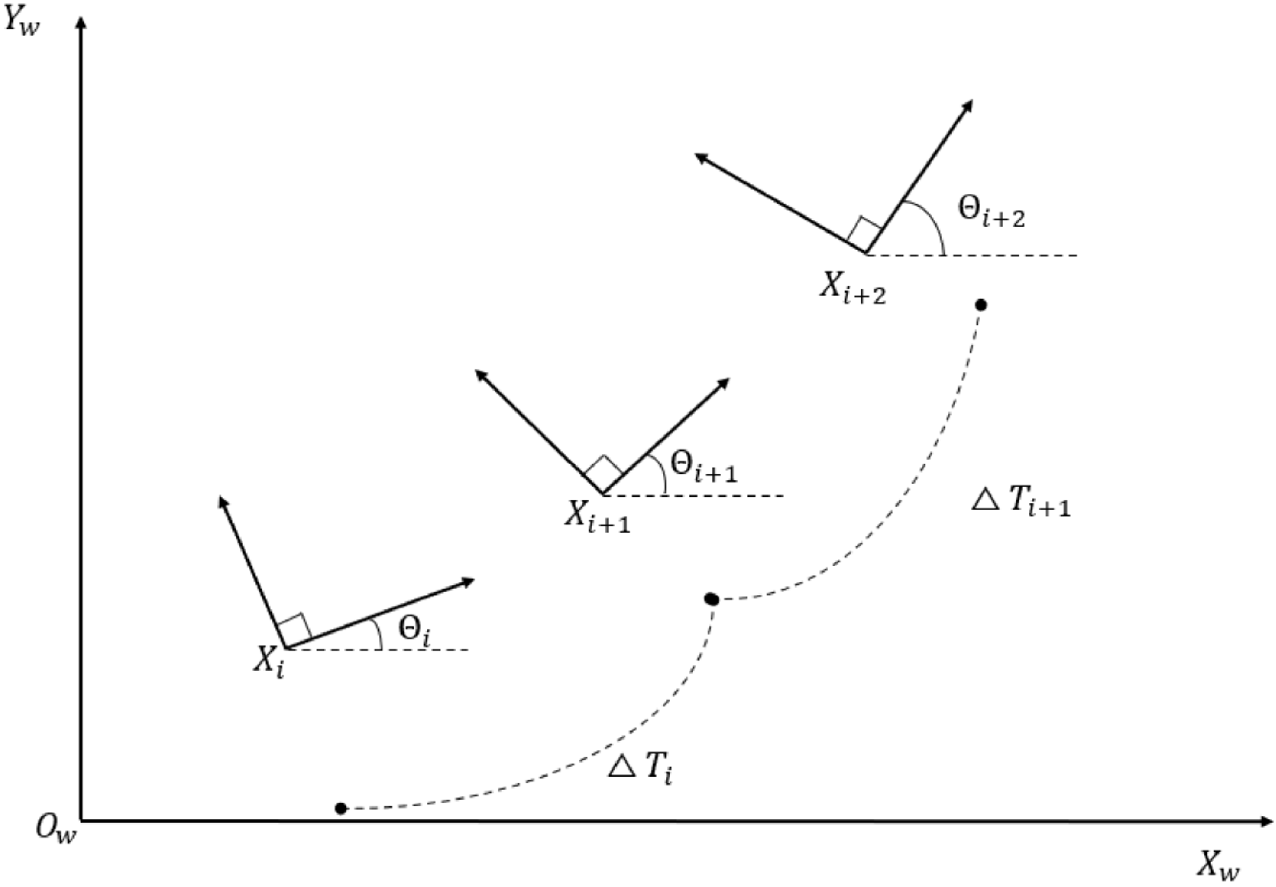
To ensure that the generated local trajectory conforms to Ackermann-steering kinematics, relevant TEB parameters for trajectory planning and obstacle avoidance were set accordingly. The minimum turning radius was defined as $\text{turning radius}=\text{wheelbase}/\tan (\text{maximum steering angle})$ , which was then incorporated as a steering constraint. In addition, penalty terms for steering angular velocity and angular acceleration were added to limit the speed and inertia of the steering mechanism. These modifications ensured that the generated local trajectory satisfied obstacle avoidance and dynamic constraints while better matching the actual steering capability of the Ackermann vehicle, thereby improving trajectory smoothness. Figure 2 showed the relationship between the robot’s poses and time intervals during motion.

Figure 2.

Pose sequence and time interval diagram of mobile robot.

Figure 2 showed the layout of the position $x_{i}$ , $y_{i}$ , and azimuth $\varTheta _{i}$ of the mobile robot at a certain state. That was, $X_{i}=(x_{i},y_{i},\varTheta _{i})^{T}$ represented the current position and orientation of the robot, and $\bigtriangleup T_{i}$ represented the time interval between two consecutive positions. From the figure, it could be seen that TEB generated n-1 time differences $\bigtriangleup T_{i}$ in two consecutive position sequences. The pose sequence $Q$ represented a series of discrete poses of the mobile robot over time during its motion. The position sequence Q was as shown in Eq. (2.c):

(2.c) \begin{equation} Q=\{X_{i}\}_{i=0.1 \ldots.. n-1} \end{equation}

Each time difference $\bigtriangleup T_{i}$ represented the time required for the robot to move from one pose to the next. The time sequence τ not only accounted for the velocity and acceleration constraints during the robot’s motion but also allowed the TEB algorithm to optimize the geometric shape of the trajectory. The set of all time differences was represented by τ as shown in Eq. (2.d):

(2.d) \begin{equation} {\unicode[Arial]{x03C4}} =\{{\unicode[Arial]{x0394}} T_{\mathrm{i}}\}_{i=0,1,\ldots ,n-1} \end{equation}

TEB was defined as a tuple of two sequences: using $B$ to represent the joint optimization of the pose sequence $Q$ and the time sequence $\tau$ , enabling the TEB algorithm to generate trajectories that were feasible both spatially and temporally, as expressed in Eq. ( 2.e):

(2.e) \begin{equation} B=(Q,{\unicode[Arial]{x03C4}} ) \end{equation}

When optimizing the TEB algorithm, it could be adjusted in real time based on the pose and time interval, and multiple objectives could be optimized simultaneously. Its solution model was expressed as Eq. (2.f):

(2.f) \begin{equation} \mathrm{f}(B)==\sum _{\mathrm{k}}{\unicode[Arial]{x03B3}} _{\mathrm{k}} \, f_{k}(B) \end{equation}

In the above equation, $f(B)$ represented the objective function, $B^{\mathrm{*}}$ was the optimized TEB trajectory, $f_{k}(B)$ was the constrained objective function, and $\gamma _{k}$ was the weight value used to measure the importance of each objective function. Considering that the constraints on linear velocity and linear acceleration were important steps in the above solution model, the constraints on linear velocity $V_{i}$ and linear acceleration $a_{i}$ were respectively Eqs. (2.g) and (2.h):

(2.g) \begin{equation} V_{i}\approx \frac{d_{i+1}}{{\unicode[Arial]{x0394}} T_{i}} \end{equation}

(2.h) \begin{equation} a_{i}\approx \frac{2{\left(V_{i+1}-V_{i}\right)}}{{\unicode[Arial]{x0394}} T_{i}+{\unicode[Arial]{x0394}} T_{i+1}} \end{equation}

In the formula, $d_{i+1}$ represented the Euclidean distance between adjacent points, and the corresponding angular velocity $\omega _{i}$ and angular acceleration constraints were $\alpha _{i}$ as shown in Eqs. (2.i) and (2.j):

(2.i) \begin{equation} \omega _{i}\approx \frac{\theta _{i+1}-\theta _{i}}{{\unicode[Arial]{x0394}} T_{i}} \end{equation}

(2.j) \begin{equation} \alpha _{i}\approx \frac{2{\left(\omega _{i+1}-\omega _{i}\right)}}{{\unicode[Arial]{x0394}} T_{i}+{\unicode[Arial]{x0394}} T_{i+1}} \end{equation}

The curvature ρ ≈ $\omega _{i}$ / $V_{i}$ . The constraint on curvature was expressed by Eq. (2.k) as follows:

(2.k) \begin{equation} f_{curv}(B)={\sum }_{i=0}^{n-1}\max (0,| p_{i}| -p_{\max })^{2} \end{equation}

The expression $max(0,x)$ indicated that a penalty was imposed when $\rho _{i}$ was greater than $\rho _{max}$ . The value of k represented the penalty coefficient, and $\rho _{max}=1/R_{min}$ . At this point, the objective function was expanded to Eq. (2.l):

(2.l) \begin{equation} f(B)=\gamma _{time} \, f_{time}(B)+\gamma _{obst} \, f_{obst}(B)+\gamma _{vel} \, f_{vel}(B)+\gamma _{curv} \, f_{curv}(B) \end{equation}

The value of $\gamma$ was all greater than or equal to 0, representing the weights of each constraint. $\gamma _{time}$ , $\gamma _{obst}$ , and $\gamma _{vel}$ , respectively, represented the weights for the time, obstacle distance, and velocity constraints. Then the final optimization objective function was Eq. (2.m):

(2.m) \begin{equation} B^{*}=\underset{B}{\arg }\min f(B) \end{equation}

3.1 Path search strategy based on dynamic heuristics

The goal of the bidirectional dynamic heuristic global planning scheme was to improve search efficiency while finding a more optimal path. In the early stage of the search, the heuristic weight function was set relatively high to reduce computational cost, and it gradually decreased in the middle and later stages, allowing the algorithm to place more emphasis on path safety and accuracy. The weight function $w(n)$ was designed to decrease progressively during the search, with $w(n)=1.0$ corresponding to the traditional A* global search; therefore, $w(n)\geq 1.0$ . The definition of $w(n)$ was given in Eq. (3.a):

(3.a) \begin{equation} w{\left(n\right)}= \begin{cases} w_{0}-\alpha \cdot \left(1-\dfrac{d_{n}}{D}\right),d_{n}\leq D\\ 1,d_{n}\gt D \end{cases} \end{equation}

In the formula, $\omega _{0}$ represented the base weight, which ensured that the search speed was accelerated in the initial stage and the search nodes were reduced. $\alpha$ was the distance attenuation coefficient, which ensured that the weight function gradually decreased as the search progresses. The range of $\alpha$ was [0,1]. When $\alpha$ was large, the weight of the path in the later stage was low, and the search efficiency was reduced. When $\alpha$ was small, there may be a situation of missing the optimal path. $d_{\mathrm{n}}$ was the Euclidean distance from the current node to the end point. D was the Euclidean distance from the starting point to the end point. The evaluation function of the Bidirectional Dynamic Heuristic A* (BI-Dynamic A*) algorithm was given in Eq. (3.b):

(3.b) \begin{align} f\left(n\right)= \begin{cases} g\left(n\right)+\left[w_{0}-\alpha \cdot \left(1-\dfrac{d_{n}}{D}\right)\right]\cdot h\left(n\right),d_{n}\leq D\\[8pt] g\left(n\right)+h\left(n\right),d_{n}\gt D \end{cases} \end{align}

According to the changes in Eq. (3.b), there was the case of Eq. (3.c):

(3.c) \begin{equation} f(n)=g(n)+(w_{0}-\alpha )\cdot h(n),d_{n}=0 \end{equation}

Based on the content of Literature [Reference Wang, Gan and Wang27], the heuristic function in the bidirectional dynamic heuristic scheme should make $(\omega _{0}-\alpha )\geq 1$ . The experimental environment was Ubuntu 20.04 system, Intel i5-12,400 CPU, NVIDIA GeForce RTX3080 graphics card, and VS Code simulation software. The improved algorithm was implemented and visualized using Python 3.8 language. The grid map of 70 m × 70 m as shown in Figure 3 was designed. The starting point and the ending point were (0,0) and (63,65), respectively.

Figure 3.

Schematic diagram of obstacles.

Since the parameters of the dynamic heuristic function only affected the search phase, their values directly influenced factors such as node expansion order, search time, and the number of expanded nodes. In contrast, path smoothing was a post-processing step performed after the search was completed and didn’t affect the search process or its computational complexity. Therefore, the optimal parameters of the dynamic heuristic function were determined prior to the path smoothing procedure. During the search phase, different parameter combinations were compared to select the dynamic heuristic parameters that achieved the best balance between search efficiency and the quality of the original path.

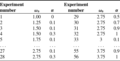
According to Eq. (3.a), the range of $\omega _{0}$ was set to [1.0,3.75] with a step size of 0.25. The range of $\alpha$ was set to [0.1,1] with a step size of 0.2. The experiments were conducted for the parameter values of $\omega _{0}$ and α to change in the groups as shown in Table I to determine the optimal parameter values.

Multiple experiments were conducted on the experimental sequence table in Table I, and the results of path length and search time for each group were shown in Figure 4.

Table I.

Experimental serial number table with different parameter values

Figure 4.

Comparison of search time and path length for different parameter values.

From the experimental data in Figure 4, it could be observed that as the parameter values increased, the path length of the BI-Dynamic A* algorithm fluctuated initially but stabilizes once the parameters exceeded a certain threshold. The main reason was that, in the constructed complex obstacle map, narrow passages impose strong constraints, resulting in highly consistent feasible paths. Variations in the dynamic heuristic function primarily affected the number of search nodes and the search time, while having limited impact on the geometric length of the generated path. As the search strategy gradually transitioned to expansions dominated by actual cost, the algorithm converged to a stable path solution, thereby reducing the differences in path length across different parameter combinations.

Experimental Groups 9 and 16 achieved the best path quality, although the differences compared with other groups were relatively small. In contrast, Experimental Group 53 outperformed the others in terms of both search time and the number of expanded nodes. Therefore, under the premise that the path length didn’t exhibit a significant disadvantage, parameter combinations with shorter search time and fewer node expansions were preferred to achieve a reasonable balance between path quality and search efficiency. In this study, Experimental Group 53 was selected, with $\omega _{0}=3.75$ and $\alpha =0.5$ .

3.2. Path smoothing

Since the dynamic heuristic function significantly reduced the heuristic weight in the later stage of the search, the generated global path became smoother in terms of curvature variation and node distribution, providing a better initial solution for subsequent TEB-based local trajectory optimization. However, geometric deficiencies still remained, making further path smoothing necessary.

3.2.2. Selection of the smoothing method

When performing secondary optimization on the path generated by the algorithm, B-spline curve smoothing or Bézier curve smoothing was commonly adopted. The advantages of Bézier curves were mainly reflected in the following aspects:

1. 1. By properly setting control points, continuity in both position and tangential direction could be ensured, which significantly reduced abrupt changes in turning angles along the path.

2. 2. The shape of a Bézier curve was constrained by its control polygon, resulting in relatively smooth curvature variation. This property facilitated subsequent curvature analysis and was well aligned with the minimum turning radius constraint of Ackermann steering.

3. 3. Structurally, a Bézier curve was determined by a finite number of control points, leading to a relatively stable computation process and easy integration into the subsequent Robot Operating System (ROS)-based planning framework. The Bézier curve equation was shown in Eq. (3.d): [Reference Guo, Wang, Wu and Sun28]

(3.d) \begin{equation} B(t)={\sum }_{i=0}^{n}({}_{i}^{n})P_{i}(1-t)^{n-i}t^{i} \end{equation}

In the formula, $P_{i}$ is expressed as the coordinate value of each point and n represents the order.

3.3. Path planning workflow for Ackermann steering

Using a bidirectional A* algorithm could improve path search efficiency and reduced computation time. This study adopted an overall collaborative search workflow combining the BI-Dynamic A* algorithm with the TEB algorithm, as shown in Figure 5.

Figure 5.

Global–local path planning flow chart.

3.4. Theoretical analysis of the BI-Dynamic A* algorithm

The dynamic heuristic function employed in this study adaptively adjusts the weight between the heuristic term and the actual cost. This mechanism enables the search strategy to dynamically tune its expansion behavior, thereby achieving an effective balance between search efficiency and path quality. Therefore, this section analyzed the theoretical properties of the proposed method from two perspectives: the boundedness of the heuristic function and the convergence behavior of the algorithm during the search process.

3.4.1. Boundedness analysis of the dynamic heuristic function

The dynamic heuristic function proposed in this study adaptively adjusted the traditional A* heuristic by introducing a distance-related weight decay mechanism with respect to the goal. Throughout the entire search process, it satisfied Eq. (3.e):

(3.e) \begin{equation} f(n)=g(n)+w(n)\cdot h(n)\leq g(n)+w_{0}\cdot h(n) \end{equation}

In Eqs. (2.b) and (3.a), $\omega (n)$ is the weighting function, which gradually decayed as the distance to the goal decreases. $\omega _{0}$ is the base weight, which monotonically decreased during the search and eventually approaches 1. This ensured that the total cost of the generated path remained controllable compared to the optimal path produced by the traditional A* algorithm. In other words, the path quality, particularly the path length, was constrained by the initial weight $\omega _{0}$ , preventing uncontrolled degradation of the path. This property provided an important guarantee for the subsequent integration with TEB-based local trajectory optimization.

4.1. Comparison of global planning methods

The comparison of global path planning trajectories in the experimental map was shown in Figure 6. (The bidirectional A* algorithm will be referred to as BI-A* in the following text; the following text simplifies BI-Dynamic Heuristic A* to BI-Dynamic A*).

Figure 6.

Algorithm path planning trajectory.

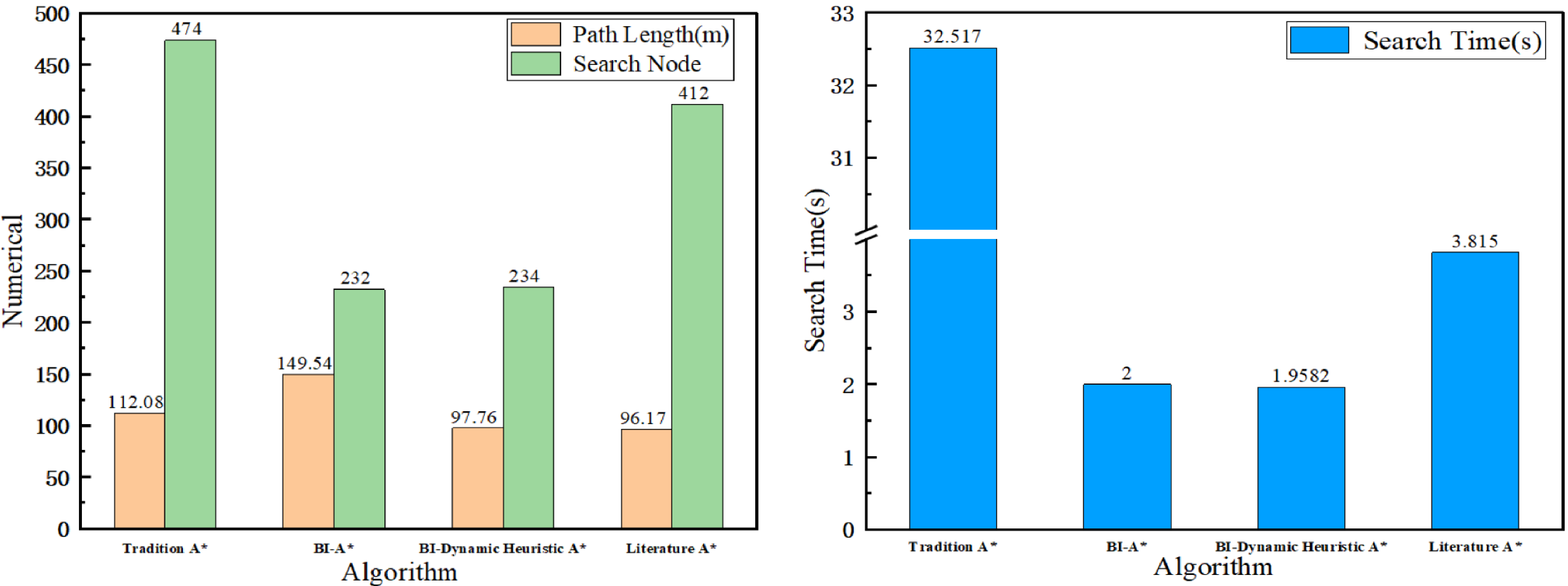
It could be observed from Figure 6 that the smoothness of the paths varies across the different algorithms. A timing function was added to each algorithm to calculate the running time for search nodes. The distances between adjacent points were then accumulated to obtain the total path length. The simulation data for the three algorithms was shown in Table II. Based on the results from Table II, Figure 7 was plotted to visually display the relevant data for each algorithm.

Table II.

Experimental simulation data of different programming algorithms

Figure 7.

Comparison of experimental results of different algorithms.

From Figure 7, it was visually clear that the BI-Dynamic A* algorithm outperforms other algorithms in terms of path length, although the number of search nodes was higher than that of the bidirectional A* algorithm. This could be attributed to the smoothing process applied to the path and the emphasis on selecting a better path, which led to a higher number of nodes being searched. However, the total number of search nodes was still fewer than that of the traditional A* algorithm and the method from Ref. [Reference Kang and Huang26]. According to Table II, the path length of the bidirectional dynamic heuristic method was reduced by 34.62% compared to bidirectional A*, and it increased by 1.653% compared to the algorithm from Ref. [Reference Kang and Huang26]. The reason for this was that, in order to balance search efficiency, the path generated by this method was not as optimal as that in Ref. [Reference Kang and Huang26], but the difference was small.

In terms of search time, the bidirectional dynamic heuristic method improved search efficiency by approximately 2.1% compared to traditional bidirectional A* and by 48.7% compared to the method in Ref. [Reference Kang and Huang26]. The number of search nodes decreased by 51.05% compared to traditional A*, increased by 0.85% compared to bidirectional A*, and decreased by 43.2% compared to the method in Ref. [Reference Kang and Huang26]. The reason for the increase in search nodes in the method from Ref. [Reference Kang and Huang26] was that it attempted 12 neighborhood searches at each intersection in search of the most optimal path, which resulted in an increase in the number of search nodes.

4.2. Model establishment of Ackerman mobile robot

The mobile robot was modeled and assembled in SolidWorks, with its components exported to URDF format. Subsequently, by configuring the xacro files for each robotic joint, the full model was constructed in ROS and imported into Gazebo for simulation. Figure 8 illustrates the state of the robot model during a turn.

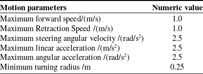
The kinematic parameters of the mobile robot were set as shown in Table III.

Table III.

Kinematic parameters of the robot

Figure 8.

Robot turning moment motion diagram in Gazebo.

4.3. ROS-based path planning engineering simulation

In this experiment, the values of $\omega _{0}$ and $\alpha$ were set to be the same as those used in the Python-based experiments. The experimental software platform was Ubuntu 20.04 with ROS Noetic. The kinematic model adopted an ideal Ackermann-steering geometry model without considering steering delay. The simulation environment focused on examining the impact of moving obstacles on the path planning scheme, assuming that the environmental perception module could provide reliable cost map inputs. This allowed for the evaluation of the feasibility and practicality of the global–local planning approach in real-world applications.

The environment maps configured in Gazebo had sizes of 15 m × 14 m and 15 m × 18 m, respectively. As shown in Figure 9, the robot started from point O at (0, 0, 0), and fixed target coordinates were issued to the robot using the rostopic command. The target points in the two environments were set to (15, 15) and (18, −12), respectively. Dynamic pedestrians were initialized at the following positions: (2, 1, 0) and (8, 7, 0) in the simple map; (5, 4, 0), (6, −5, 0), and (16, −3, 0) in the complex map. All pedestrians were programmed to follow cyclic motion based on predefined time schedules and coordinate sequences. The grid maps displayed in RViz are shown in Figure 9 (b) and (d), where white regions indicated traversable areas and black regions represented obstacle regions.

Figure 9.

Map models in a simulation environment.

4.4. Comparison of global path planning simulation results

The ROS Toolbox in MATLAB provided a bidirectional interface between Simulink and ROS, enabling joint simulation with ROS [Reference Zhang, Qi, Zhang and Li29]. In this experiment, the /odom topic was subscribed to MATLAB to display the robot’s position changes in real time. A top-down screenshot of the Gazebo simulation environment was loaded into MATLAB, and the robot’s motion trajectory in ROS was plotted in real time to facilitate the evaluation of the path planning performance. The relationships between the x and y axes in MATLAB and the transformations were defined as follows: $w_{x}$ and $w_{y}$ represented the width and height of the displayed image, and $l_{x}$ and $l_{y}$ represented the lengths of the map in Gazebo along the x and y axes, respectively. The relationships were given by Eqs. (4.a) and (4.b):

(4.a) \begin{equation} X_{f}=\frac{M_{w}}{G_{y}} \end{equation}

(4.b) \begin{equation} Y_{f}=\frac{M_{h}}{G_{x}} \end{equation}

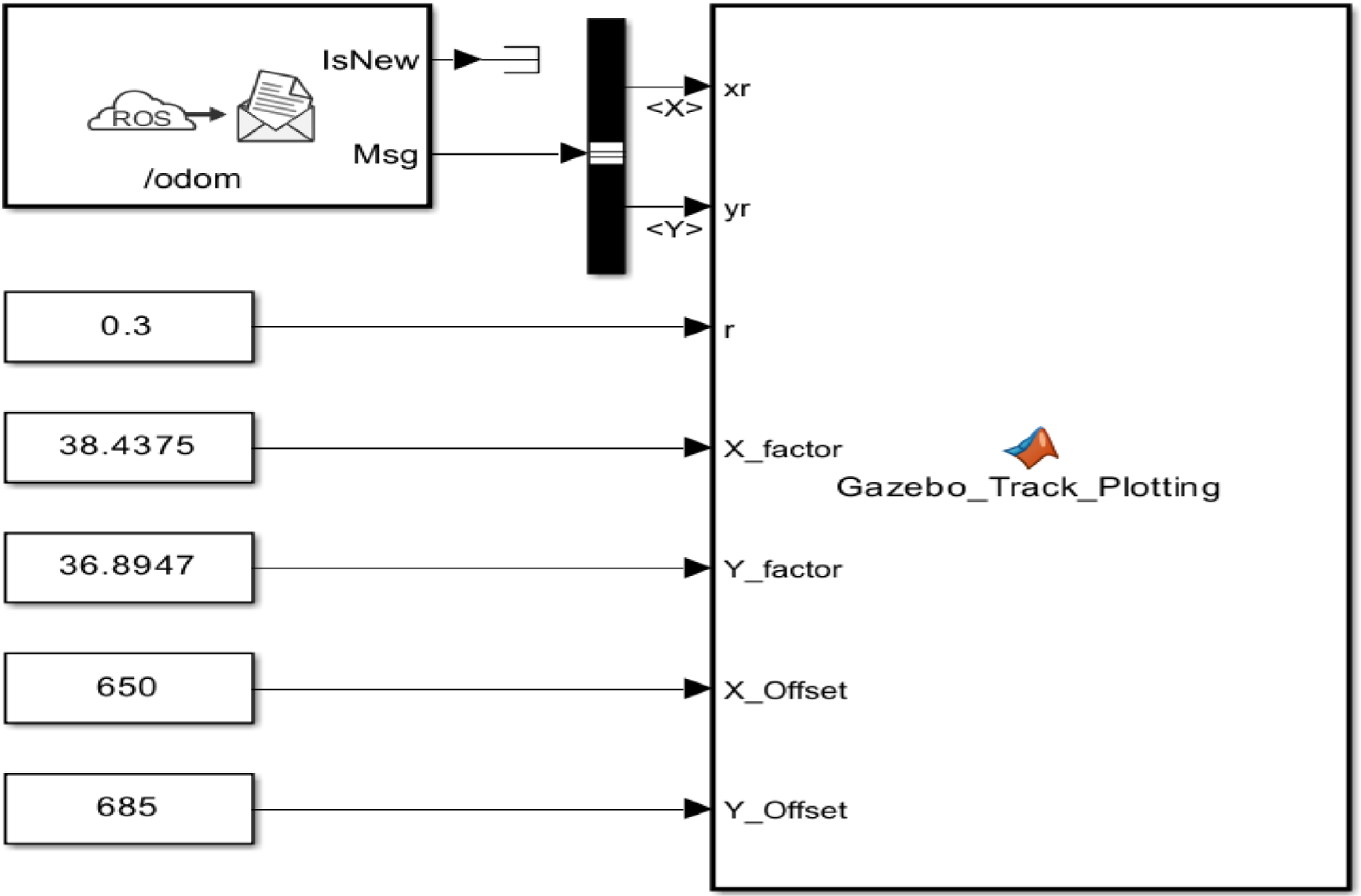
The X_Offset and Y_Offset represented the offsets of the robot along the x-axis and y-axis, respectively. The Simulink module and the values of each parameter are shown in Figure 10.

Figure 10.

Design of Simulink trajectory drawing module.

Figure 10 Long description

The diagram illustrates the design of a Simulink trajectory drawing module. It features a ROS odom message with IsNew and Msg components, connected to a block that outputs xr and yr values. Below this block, there are labeled values for 0.3, 38.4375, 36.8947, 650, and 685, which correspond to r, X_factor, Y_factor, X_Offset, and Y_Offset respectively. These values are connected to a Gazebo_Track_Plotting block, indicating the flow of data and parameters within the module.

The coordinate system directions of MATLAB and Gazebo were related as shown in Figure 11. By adjusting the value of the offset, ensured that the origin positions of MATLAB and Gazebo were corresponding, and the position of the coordinate system O point was the corresponding position of the Gazebo robot.

Figure 11.

Design of Simulink trajectory drawing module.

Figure 11 Long description

The image consists of two parts. The first part is a diagram illustrating the frame transform between MATLAB and Gazebo. It shows the X-axis and Y-axis directions in both MATLAB and Gazebo, with arrows indicating the direction of each axis. The second part is a top-down screenshot in MATLAB, displaying a grid with walls and obstacles. The screenshot includes labeled axes with X and Y directions, and a coordinate point marked as (0, 0).

In the ROS simulation environment, after the global planner generates a path, discrete path points were automatically extracted by subscribing to the global path topic, and path curvature and other geometric metrics were calculated based on adjacent path points. Multiple independent planning experiments were conducted in the same simulation environment. As shown in Figure 12(a) and (d), the global planning routes of traditional bidirectional A* and bidirectional dynamic heuristic algorithms are represented, respectively.

Figure 12.

Comparison of global and local algorithm trajectories.

Figure 12 Long description

The image contains six diagrams comparing global and local algorithm trajectories in a grid environment with obstacles. The diagrams are arranged in two rows and three columns. The first row shows the global paths planned by BI-A* and BI-Dynamic A* algorithms, respectively. The second row displays the actual trajectories with traditional TEB and the actual trajectory of the TEB algorithm. Each diagram features a red line representing the path or trajectory, a grid layout indicating the environment, and various obstacles depicted as black rectangles. The axes are labeled X and Y, with an origin point marked O. The diagrams illustrate how different algorithms navigate through the environment, highlighting variations in path planning and trajectory execution.

The global path was generated by the BI-Dynamic A* algorithm and output as discrete waypoints. To quantitatively analyze its geometric properties, a discrete curvature model based on three adjacent points was employed to perform a statistical analysis of the path’s curvature distribution. The experimental results in Figure 12 showed that the generated path exhibits smoother curvature changes in the turning areas, providing a good initial condition for the subsequent TEB local trajectory optimization. (In this paper, the TEB planning scheme was represented as I-TEB.)

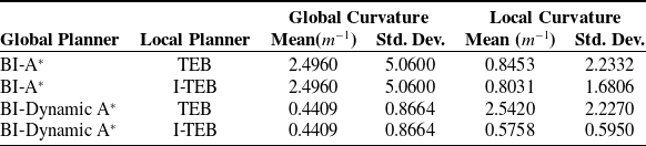
Since global path planning may be affected by path pruning and replanning mechanisms, the number of generated path points could vary at different stages. To ensure the representativeness of the statistics, the analysis was based on the first generated global path, and only paths with a number of points not less than 80% of the original path length were selected for curvature statistics. This approach reflected the overall geometric characteristics of the global path. For TEB-based local planning, the average curvature of the trajectories generated by TEB was calculated as an indicator of overall trajectory smoothness. The experimental results for the entire motion process were summarized in Table IV.

Table IV.

Path curvature statistics for various algorithms

Based on the data in Table IV, Figure 13 was plotted to visually illustrate the curvature variations for different algorithm combinations.

Figure 13.

Mean and standard deviation of curvature for different algorithm combinations

Figure 13 Long description

The image contains two bar graphs comparing curvature values for different algorithms. The first graph, labeled as Global curvature comparison, shows average curvature and curvature standard deviation for BI-Dynamic A* and BI-A*. BI-Dynamic A* has an average curvature of 0.4409 and a standard deviation of 0.8664, while BI-A* has an average curvature of 2.496 and a standard deviation of 5.06. The second graph, labeled as local curvature comparison, compares TEB and I-TEB algorithms for BI-Dynamic A* and BI-A*. The TEB algorithm for BI-Dynamic A* shows higher curvature values with more variability, while the I-TEB algorithm shows lower and more consistent curvature values. For BI-A*, the TEB algorithm also shows higher curvature values with more variability compared to the I-TEB algorithm. The graphs illustrate the differences in curvature performance between the algorithms.

In the ROS simulation experiment, the curvature of the local trajectories generated by the TEB local planner during the stable motion phase was statistically analyzed.

To mitigate the impact of trajectory degradation near the goal and local optimization anomalies on the statistical results, this study only analyzed local trajectory segments that contained more than 10 waypoints and where the robot was in a stable motion state. The results show that the BI-Dynamic A* algorithm effectively reduced unnecessary twists in the global path. The generated trajectories had an average curvature of approximately 0.4409 and a curvature standard deviation of 0.8664. Additionally, the TEB planner, as compared to the traditional TEB, further suppressed the curvature fluctuations in the local trajectory. The experimental results showed that the standard deviation of curvature exceeded its mean value. This is attributed to the inherent piecewise-linear nature of the global planner and the presence of certain turning points in the path, both contributing to the increased variance in curvature values. Through the collaborative optimization of the global and local planners, the motion stability and executability of the Ackermann robot have been effectively improved.

4.5. Impact analysis based on TEB trajectory optimization

In Figure 14, the red line represents the global path planning effect displayed by the four algorithms in Rviz. At this point, the robot has not yet started moving.

Table V.

Simulation data of different planning algorithms

Figure 14.

Comparison of robot trajectories under simple and complex maps.

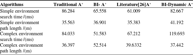
Simulation data were obtained by averaging 10 experiments on the computation time and optimal path length of the three algorithms, as shown in Table V and Figure 15.

Figure 15.

Simulation data of different planning algorithms.

The simulation data of the experiment, as presented in Table V and Figure 14, were obtained by averaging the results of 10 trials. These trials measured the time required for generating global planning paths and the length of the optimal paths produced by the execution files of three distinct algorithms.

Based on Table V, a scatter plot as shown in Figure 15 was drawn.

From Figure 15, it was clear that the BI-Dynamic A* algorithm outperforms other algorithms in both path length and search efficiency. According to Table IV, in the simple environment group, the BI-Dynamic A* algorithm improved search time by about 29.3% compared to traditional A*, and by 6.93% and 26.19% compared to the bidirectional A* and the algorithm from Ref. [Reference Kang and Huang26], respectively. The optimization effect of BI-Dynamic A* in the experiment was slightly improved compared to other algorithms due to the relative simplicity of the map environment compared to the Python-based environment. However, overall, BI-Dynamic A* performed better than bidirectional A* in terms of path length and better than traditional A* in search time, consistent with the conclusions from Python-based experiments. The path length generated by BI-Dynamic A* was improved by 4.11% and 14.10% compared to bidirectional A* and the algorithm from Ref. [Reference Kang and Huang26], respectively, with only a small difference compared to the traditional A* path length. In the complex environment group, the search time of BI-Dynamic A* was improved by 20.01% and 43.84% compared to traditional A* and the algorithm from Ref. [Reference Kang and Huang26], but it was slightly higher than bidirectional A*. The reason for this was that BI-Dynamic A* guarantees a more optimal path selection, which led to a longer search time compared to bidirectional A*. The path length generated by BI-Dynamic A* was improved by 24.52% compared to bidirectional A*, but still longer than the paths generated by traditional A* and the algorithm from Ref. [Reference Kang and Huang26]. This was because BI-Dynamic A* tended to generate smoother paths, leading to relatively longer paths.

To verify the differences between the TEB planning scheme, traditional TEB algorithm, and DWA algorithm, the robot’s linear and angular velocities during motion were output by subscribing to the cmd_vel topic in the ROS environment. Around 40s, the TEB planning scheme group reached the target point, while the DWA algorithm has not yet arrived. The kinematic characteristic curves of the TEB planning scheme group, traditional TEB, and DWA algorithm groups were analyzed by selecting the time range when the TEB planning scheme group reached the target point. (The TEB planning scheme is represented as I-TEB.) The speed variation in both maps was shown in Figures 16 and 18.

Figure 16.

Changes in the linear and angular velocities of the robot under simple maps.

Table VI.

Different algorithms combine linear velocity and angular velocity change

Figure 17.

Variations in linear velocity and angular velocity on a simplified map.

Figure 18.

Changes in the linear and angular velocities of the robot under complex maps.

Due to dynamic obstacles in the map, the robot’s motion trajectory differs, and the robot may deviate from the global planned path. Therefore, the path tracking error index was used to evaluate the global system’s stability, not just the local stability. The robot’s actual trajectory was obtained from the /odom topic in ROS, while the reference path was provided by the global path topic. The minimum Euclidean distance between the robot’s actual position and the global reference path was calculated as the instantaneous tracking error. The average error was then statistically computed to quantify the path’s trackability.

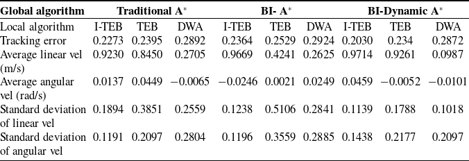
The mean values and standard deviations of linear velocity and angular velocity under various experimental combinations on a simplified map were presented in Table VI.

The data presented in Table VI were graphically illustrated in Figure 17.

As can be observed from Figure 17, the I-TEB group exhibited a lower standard deviation of angular velocity than the other groups, indicating smaller velocity fluctuations and smoother motion. According to the results in Table VI, the average linear velocity of the I-TEB group was higher than that of the DWA algorithm. The reason for this difference was that the DWA algorithm prioritizes optimal local safety. This focus leads it to adopt a lower linear velocity, resulting in longer planning time. In contrast, the TEB algorithm discretized the global path into multiple pose points and optimizes them. This allows it to select a higher speed while ensuring safety, thereby saving planning time. The I-TEB algorithm achieved efficient linear motion, with an average angular velocity of approximately 0.02 rad/s, indicating smooth steering behavior. Although the traditional TEB algorithm reached a linear velocity of 0.9 m/s in the conventional A* group, its angular velocity standard deviation was as high as 0.21, leading to significant fluctuations and unstable robot motion.

The path tracking error for the BI-Dynamic A* algorithm was slightly lower than that of traditional A* and bidirectional A*, primarily because BI-Dynamic A* emphasizes path smoothness, which results in better curvature variation and geometric continuity. This made the planned path more suitable for vehicle kinematics. During dynamic obstacle avoidance, the robot frequently adjusted its global path, which led to some deviation between the actual motion trajectory and the global path. However, in the local planning algorithm group, the TEB planning scheme outperformed both traditional TEB and DWA, demonstrating better local planning performance.

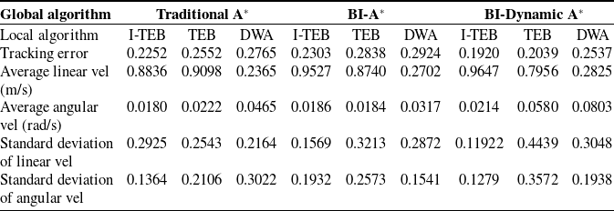
The variations of linear velocity and angular velocity of the mobile robot under different algorithm combinations in complex maps were shown in Table VII.

Table VII.

Different algorithms combine linear velocity and angular velocity change

Based on the data presented in Table VII, the corresponding graph was illustrated in Figure 19.

Figure 19.

Changes in linear velocity and angular velocity under complex maps.

From Figure 19, it could be visually observed that in the complex map, the I-TEB group had a lower standard deviation of angular velocity compared to other groups, indicating smaller velocity fluctuations and smoother motion. According to Table VII, in the BI-Dynamic A* group, the DWA group had an average linear velocity of only 0.0987 m/s. This was because the DWA algorithm tends to lower the linear velocity and frequently adjusted the robot’s orientation in the velocity space to ensure local safety, which led to a reduction in overall motion efficiency. This phenomenon suggested that when DWA was coupled with high-quality geometric paths, it was difficult to fully leverage the advantages of global planning. The TEB algorithm performed well under most global algorithms, with efficient linear velocity and an average angular velocity of about 0.02 rad/s, resulting in smooth steering. In contrast, the traditional TEB algorithm in the traditional A* group had a linear velocity of 0.845 m/s but a high linear velocity standard deviation of 0.3851, causing large fluctuations and leading to unstable robot motion. In terms of path tracking error, the TEB-based groups generally exhibited lower tracking errors. On the other hand, the DWA group, due to frequent orientation adjustments, showed larger velocity fluctuations and an increase in path tracking error.

These results demonstrate that introducing a minimum turning radius constraint, together with high-quality global path geometric properties, was a key factor in reducing path tracking error and enhancing the motion stability of Ackermann-steered robots.

4.6. Trajectory analysis of edge cases in complex maps

To validate the effectiveness of the proposed method, this section analyzed edge cases in complex maps where the robot encountered dynamic pedestrians and sharp turns, which may cause abrupt changes in linear and angular velocities. The variations in linear velocity, angular velocity, and curvature under different algorithm combinations in these edge scenarios were comparatively analyzed, as illustrated in Figure 20.

Figure 20.

Local trajectories in edge-case scenarios.

Based on the overall variation trends in Figure 18, the velocity and angular velocity curves for edge-case scenarios were illustrated in Figure 21, while Figure 22 presents the three-dimensional visualization of the curvature constraints.

Figure 21.

Edge-case velocity curves.

Figure 22.

3D visualization of curvature constraints in edge cases.

From the results in Figure 21, it could be clearly observed that, under edge-case scenarios, the linear velocity mainly remained within 1.0 m/s, while the angular velocity reached a maximum of about 1.15 rad/s and a minimum of approximately −1.5 rad/s. Overall, the motion profiles satisfied the predefined robot constraints.

Further analysis with the three-dimensional surface plot in Figure 22 revealed that the path generated by traditional A* had good smoothness but was limited in search efficiency. Traditional bidirectional A* improved efficiency, but the curvature fluctuated significantly. In contrast, the BI-Dynamic A* algorithm ensured both search efficiency and smoother curvature changed over time and linear velocity. The curvature variation in the time–velocity plane was more gradual, leading to a more continuous curvature with the robot’s movement and reflecting better path quality. Compared to bidirectional A*, the curvature in the traditional A* group changed more smoothly over time and velocity, with overall fluctuations being smaller. On the other hand, the bidirectional A* group showed more drastic curvature changes, with noticeable high-curvature areas, indicating poorer path smoothness.

4.7. Real environment experiments

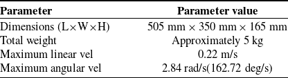
Due to the idealized radar distance measurement errors in the simulation environment, there were some differences when applied to a real-world environment. This study evaluated the obstacle avoidance capability of the path planning scheme in a real environment. The robot used was the Qingzhou YQ01, an Ackermann model, equipped with a multi-sensor fusion system. This mobile robot was equipped with a Jeton NANO controller and LiDAR, enabling dynamic path planning and obstacle avoidance capabilities. The mobile robot model diagram and performance parameter table were shown in Figure 23 and Table VIII.

Figure 23.

Aerospace light boat robot model diagram.

By utilizing the visualization tool Rviz, the target point for the robot was established, and the robot’s obstacle avoidance performance was observed, as illustrated in Figure 24: the global planning route was indicated by the red line, while the local planning route was denoted by the green line.