





1. Introduction
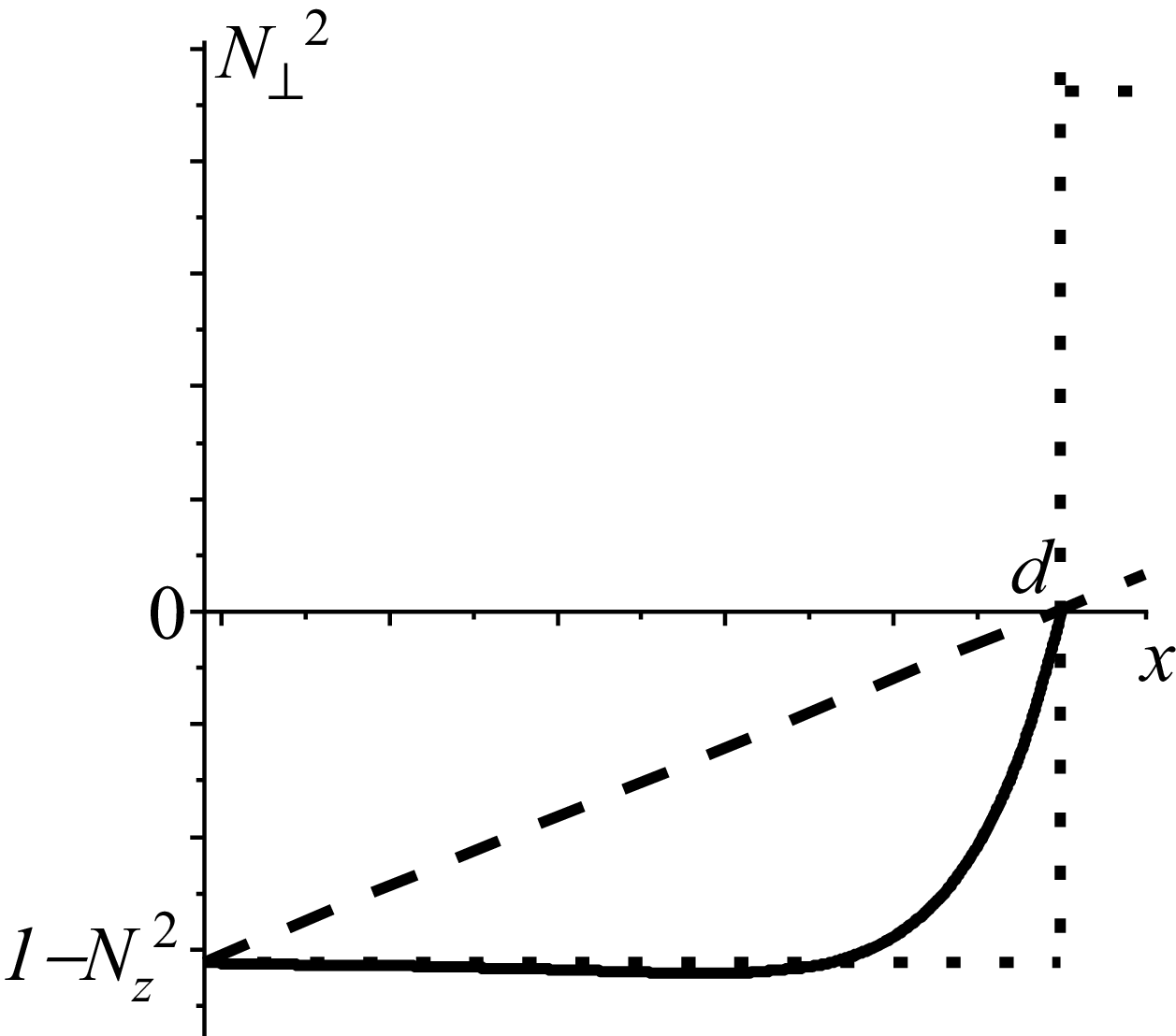
Fast magnetosonic wave (FMSW) attenuation in toroidal plasmas was initially studied in the framework of the simplest model (see, e.g. Bhatnagar et al. Reference Bhatnagar, Evrard, Faulconer, Geilfus, Koch, Luwel, Messiaen, Pearson, Vandenplas and Weynants1982), which was the step model. Within this model, plasma density was assumed to be zero in an evanescent layer in front of the antenna and then sharply increased to a value higher than the cutoff density at a distance of
 $d$
from the antenna (see dotted line in figure 1). In this approach, the fraction of the transmitted power strongly depends on the plasma density at the step. In figure 1, the square of the perpendicular refractive index of the FMSW in the cold plasma approximation is
Schematic evolution of
 ${N}_{\bot }^{2}(x)$
in three different cases: step plasma density (dotted line), linear evolution of
 ${N}_{\bot }^{2}(x)$
like in Bilato et al. (Reference Bilato, Brambilla, Hartmann and Parisot2005) (dashed line), linear evolution of plasma density (solid curve).

 \begin{align}{N}_{\bot }^{2}=\frac{(S-{N}_{z}^{2})^{2}-D^{2}}{S-{N}_{z}^{2}}.\end{align}
In (1.1),
 $S$
and
 $D$
are the components of cold collisionless plasma dielectric permittivity tensor (the so-called Stix parameters, see Stix Reference Stix1992) and
 $N_{z}=k_{z}/k_{0}$
is the toroidal refractive index, where
 $k_{z}$
is the toroidal wavenumber,
 $k_{0}=\omega /c$
is the vacuum wavenumber,
 $\omega$
is an antenna operating angular frequency and
 $c$
is the speed of light in vacuum. In the ion cyclotron frequency range,
 $\omega _{ci}\lesssim \omega \ll | \omega _{ce}|$
, the components of the plasma dielectric permittivity tensor read
 \begin{align}S=1-\sum _{\alpha }\frac{{\omega }_{p\alpha }^{2}}{\omega ^{2}-{\omega }_{c\alpha }^{2}}, \quad D=\sum _{\alpha }\frac{{\omega }_{p\alpha }^{2}\omega _{c\alpha }}{\omega \left(\omega ^{2}-{\omega }_{c\alpha }^{2}\right)}.\end{align}
In (1.2), the summation is carried out by plasma particle species,
 $\alpha =i$
for ions and
 $\alpha =e$
for electrons,
 $\omega _{c\alpha }=Z_{\alpha }eB_{0}/(m_{\alpha }c)$
and
 $\omega _{p\alpha }=(4\pi n_{\alpha }{Z}_{\alpha }^{2}e^{2}/m_{\alpha })^{1/2}\,$
are the cyclotron and plasma frequencies, respectively,
 $e$
is the elementary electric charge,
 $B_{0}$
is the toroidal static magnetic field for which the spatial dependence is neglected,
 $Z_{i}$
is the ion charge state and
 $m_{\alpha }$
is the particle mass.
Further studies considering more realistic plasma density profiles described the FMSW attenuation in the evanescent layer near the antenna in terms of the exponential factor
 $\exp (-2\kappa d)$
(see, e.g. Bhatnagar et al. Reference Bhatnagar, Evrard, Faulconer, Geilfus, Koch, Luwel, Messiaen, Pearson, Vandenplas and Weynants1982; Mayberry et al. Reference Mayberry, Chiu, Pinsker, Prater, Hoffman, Baity, Ryan and Uesugi1990; Ikezi & Phelps Reference Ikezi and Phelps1997). Here,
 $\kappa ^{2}={k}_{z}^{2}+{k}_{y}^{2}-{k}_{0}^{2}\gt 0$
, where
 $k_{y}$
is the poloidal wavenumber. This dependence of attenuation factor was demonstrated for FMSWs with
 $k_{y}=0$
to be too pessimistic with an elementary one-dimensional model in Bilato et al. (Reference Bilato, Brambilla, Hartmann and Parisot2005), where
 ${k}_{\bot }^{2}={k}_{0}^{2}{N}_{\bot }^{2}$
was considered to be linear function of the coordinate
 $x$
(see dashed line in figure 1)
 \begin{align}{k}_{\bot }^{2}={k}_{0}^{2}\frac{x}{L_{n}}+{k}_{\bot }^{2}(0).\end{align}
In (1.3),
 $L_{n}=-d/{N}_{\bot }^{2}(0)$
. In this case
 ${k}_{\bot }^{2}(x)$
varied linearly from some
 ${k}_{\bot }^{2}(0)\lt 0$
at the antenna,
 $x=0$
, to zero at the cutoff,
 $x=d$
.
The present paper generalises the considerations of Bilato et al. (Reference Bilato, Brambilla, Hartmann and Parisot2005) by accounting for non-zero poloidal wave refractive index. A slab model is utilised. Spatial evolution of the FMSW
 $E_{y}$
poloidal electric field amplitude in a tokamak scrape off layer is determined in § 2 with application of asymptotic methods for FMSWs with
 $k_{y}=0$
. The asymptotic expressions for the
 $E_{y}$
field amplitudes are matched and the fraction of the transmitted power is determined in terms of optical thickness of the evanescent layer in § 3. The results obtained in §§ 2 and 3 are generalised to the case of FMSWs with
 $k_{y}\neq 0$
in § 4. The fraction of the transmitted power is analysed numerically as a function of the plasma density decay length subject to toroidal and poloidal refractive indices, plasma density at the antenna and operating frequency in § 5. Spatial evolution of the
 $E_{y}$
field amplitude is presented in § 5 as well. The main results are summarised in the Conclusions. Appendices A–C present the detailed derivation of the asymptotic expressions for the FMSW
 $E_{y}$
field amplitude in a low-density tokamak plasma. Technical details of the dependence of the evanescent layer thickness on the plasma density decay length are provided in Appendix D.
Although the present paper contributes to the development of FMSW theory, it is not without its shortcomings. In particular, coupling between fast and slow waves is ignored based on the infinite plasma conductivity in the toroidal direction. The assumption significantly simplifies calculations, but excludes the variety of physical phenomena which can be observed in the strongly non-uniform plasma of a tokamak scrape off layer like confluences, mode conversion, the excitation of surface waves on steep gradients, etc. Therefore, the present paper cannot be considered as a complete and definitive solution to the problem of the electromagnetic wave dynamics in the low-density edge plasma of a tokamak.
2. Wave field spatial evolution in a tokamak scrape off layer
A FMSW with
 $k_{y}=0$
and
 $| k_{z}| \gt k_{0}$
like in Bilato et al. (Reference Bilato, Brambilla, Hartmann and Parisot2005) is considered initially. Outgoing boundary conditions are applied on the side of the plasma, such that no electromagnetic signal comes back from the plasma core. In the following, the exponential plasma density variation is considered (see Stangeby Reference Stangeby2000)
 \begin{align}n(x)=n(d)\exp [(x-d)/\lambda ].\end{align}
In (2.1),
 $\lambda$
is the plasma density decay length,
 $n(d)$
is plasma density at the cut-off. Plasma density is
 $\exp (d/\lambda )$
times higher at the cutoff,
 $x=d$
, than at the antenna,
 $x=0$
. Note, that the width of evanescent layer
 $d$
is different for FMSWs with different toroidal refractive indices, i.e.
 $d$
is a function of
 $N_{z}$
,
 $d=d({N}_{z}^{2})$
.
Maxwell’s equations provide the following ordinary linear uniform second-order differential equation for the FMSW
 $E_{y}(x)$
amplitude (neglecting the wave toroidal electric field,
 $E_{z}=0$
)
 \begin{align}\frac{{d^{2}}E_{y}}{{\rm d}x^{2}}+{k}_{\bot }^{2}E_{y}=0.\end{align}
We separate the space of a tokamak scrape off layer into three overlapping regions. The first one starts at an antenna,
 $x=0$
, where the plasma density is assumed to be sufficiently small, such that in a plasma containing ions of a single species and electrons, the following inequality is realised:
 $n(x)\ll ({N}_{z}^{2}-1)(1+\varphi )m_{i}{\omega }_{ci}^{2}/(4\pi e^{2})$
. Here, and hereinafter,
 $\varphi =\omega /\omega _{ci}$
. Within this region,
 $1-S\ll 1$
, and
 $D\ll 1$
. This region is almost all evanescent region,
 ${N}_{\bot }^{2}\lt 0$
, except of the narrow region nearby the cutoff,
 ${N}_{\bot }^{2}=0$
. The second region is around the cutoff,
 ${N}_{\bot }^{2}\approx 0$
. Within this region, deviation of
 ${N}_{\bot }^{2}$
evolution with the coordinate
 $x$
from linearity is weak. The third region is that where
 ${N}_{\bot }^{2}\gg ({N}_{z}^{2}-1)(1+\varphi )$
and is approximately proportional to the plasma density,
 ${N}_{\bot }^{2}(x)\propto n(x)$
.
2.1. Wave field evolution in the first region
The wave field amplitude is searched by asymptotic methods (see, e.g. Fedoryuk Reference Fedoryuk1993). Within the first region, exponential functions are chosen as the reference ones
 \begin{align}E_{y}=A_{1}(x){\exp}(-\chi (x))+A_{2}(x)\exp (\chi (x)).\end{align}
The reason to choose just exponential functions as reference ones is as follows. In a zero-density plasma,
 ${N}_{\bot }^{2}=1-{N}_{z}^{2}$
, and (2.2) can be solved precisely in terms of exponential functions,
 $E_{y}=A_{1}\exp (-\kappa x)+A_{2}\exp (\kappa x)$
, with
 $A_{1,2}$
being the constants of integration. Accounting for plasma density variation in the evanescent layer needs application of the method of reference equations, taking the exponent as the reference function and assuming that the amplitudes
 $A_{1,2}(x)$
are slowly varying functions of the coordinate
 $x$
. Some algebra provides that
 \begin{align}\chi (x)={\int }_{0}^{x}\kappa _{\bot }{\rm d}x,\,{\rm and}\, A_{1,2}(x)\propto {\kappa _{\bot }}^{-1/2}.\end{align}
In (2.4),
 $\kappa _{\bot }(x)\equiv \sqrt{-{k}_{\bot }^{2}(x)}$
. Consequently, the wave field amplitude reads
 \begin{align}{E}_{y}^{\left(1\right)}=\frac{1}{\sqrt{\kappa _{\bot }}}\left[A_{11}\exp \left({\int }_{0}^{x}\kappa _{\bot }{\rm d}x\right)+A_{12}\exp \left(-{\int }_{0}^{x}\kappa _{\bot }{\rm d}x\right)\right].\end{align}
In (2.5),
 $A_{11,12}$
are the constants of integration. The notation ‘(1)’ in ‘
 ${E}_{y}^{(1)}$
’ in (2.5) means that the expression is valid within the first region. The solution (2.5) is well known as the Wentzel–Kramers–Brillouin (WKB) approximation. Detailed derivation of expression (2.5) is presented in Appendix A.
2.2. Wave field evolution in the second region
The second region is characterised by the presence of the cutoff,
 ${k}_{\bot }^{2}=0$
, at
 $x=d$
. That is why Airy functions
 $\mathrm{Ai}(\xi )$
and
 $\mathrm{Bi}(\xi )$
are chosen as the reference ones (see page 446 in Abramowitz & Stegun Reference Abramowitz and Stegun1964). Application of asymptotic methods described e.g. in Fedoryuk (Reference Fedoryuk1993) makes it possible to take into account possible deviation of
 ${k}_{\bot }^{2}$
in (2.2) from linearity by modifying the argument
 $\xi (x)$
and introducing the dependence of amplitude
 \begin{align}{E}_{y}^{(2)}=\frac{1}{\sqrt{-{\rm d}\xi /{\rm d}x}}\left[B_{1}\mathrm{Ai}(\xi (x))+B_{2}\mathrm{Bi}(\xi (x))\right].\end{align}
In (2.6),
 $B_{1,2}$
are integration constants
 \begin{align}\xi (x)=\begin{cases} \xi (x)=\left(-\dfrac{3}{2}{\displaystyle\int }_{\kern-4pt d}^{x}\sqrt{{-k}_{\bot }^{2}}{\rm d}x\right)^{2/3},\,{i\kern-2pt f}\,x\lt d;\\[12pt] \xi (x)=-\left(\dfrac{3}{2}{\displaystyle\int }_{\kern-4pt d}^{x}\sqrt{{k}_{\bot }^{2}}{\rm d}x\right)^{{2}/{3}},\,{i\kern-2pt f}\,x\gt d. \end{cases}\end{align}
The notation ‘(2)’ in ‘
 ${E}_{y}^{(2)}$
’ in (2.6) means that the expression is valid within the second region. One can find the detailed derivation of expression (2.6) in Appendix B.
2.3. Wave field evolution in the third region
This asymptotic presentation (2.6) deviates from precise one for large negative arguments, where
 ${k}_{\bot }^{2}$
increases almost exponentially. Replacement of
 ${k}_{\bot }^{2}$
in (2.2) by
 ${k}_{\bot }^{2}(d)\exp [(x-d)/\lambda ]$
(with
 $\lambda$
being the plasma density decay length) transforms it to a Bessel equation of order zero. This makes it possible to search the wave electric field amplitude in this region in the following asymptotic form:
 \begin{align}{E}_{y}^{(3)}=C_{1}(x)J_{0}(p(x))+C_{2}(x)Y_{0}(p(x)).\end{align}
The notation ‘(3)’ in ‘
 ${E}_{y}^{(3)}$
’ in (2.8) means that the expression is valid within the third region. In (2.8),
 $J_{0}(p)$
and
 $Y_{0}(p)$
are Bessel functions of the first kind of the zeroth order (see page 358 in Abramowitz & Stegun Reference Abramowitz and Stegun1964);
 $C_{1,2}(x)$
are relatively slowly varying functions of the coordinate
 $x$
 \begin{align}C_{1,2}(x)=C_{11,12}\sqrt{\frac{{\int }_{\kern-4pt d}^{x}k_{\bot }{\rm d}x}{k_{\bot }}}, p(x)={\int }_{\kern-4pt d}^{x}k_{\bot }{\rm d}x.\end{align}
In (2.9),
 $C_{11,12}$
are the constants of integration. A detailed explanation of how to derive expressions (2.8) and (2.9) is presented in Appendix C. The coefficient
 $C_{12}$
is chosen in the following as
 $iC_{11}$
to satisfy the outgoing boundary condition at
 $x\rightarrow +\infty$
, where the FMSW should propagate in the positive direction without reflection from the core plasma.
3. Matching the asymptotic solutions
3.1. Matching the asymptotic solutions between the second and the third regions
To match the asymptotic solutions (2.6) and (2.8), one needs asymptotic representations of Airy functions of large negative argument (see pages 448 and 449 in Abramowitz & Stegun Reference Abramowitz and Stegun1964)
 \begin{align}\mathrm{Ai}(-\xi (x))\approx \frac{\sin (({2}/{3})(-\xi)^{({3}/{2})}+({\pi }/{4}))}{\sqrt{\pi }(-\xi)^{1/4}}, \mathrm{Bi}(-\xi (x))\approx \frac{\cos (({2}/{3})(-\xi)^{({3}/{2})}+({\pi }/{4}))}{\sqrt{\pi }(-\xi)^{1/4}},\end{align}
as well as asymptotic presentations of Bessel functions of large argument (see page 364 in Abramowitz & Stegun Reference Abramowitz and Stegun1964)
 \begin{align}J_{0}(p)\approx \sqrt{\frac{2}{\pi p}}\cos \left(p-\frac{\pi }{4}\right),\quad Y_{0}(p)\approx \sqrt{\frac{2}{\pi p}}\sin \left(p-\frac{\pi }{4}\right).\end{align}
Substituting the expressions (3.1)–(3.12) into (2.6) and (2.8) provides
 \begin{align} {E}_{y}^{(2)}&\approx \frac{1}{\sqrt{\pi k_{\bot }}}\left[B_{1}\cos \left({\int }_{\kern-4pt d}^{x}k_{\bot }{\rm d}x-\frac{\pi }{4}\right)-B_{2}\sin \left({\int }_{\kern-4pt d}^{x}k_{\bot }{\rm d}x-\frac{\pi }{4}\right)\right],\\[-10pt]\nonumber\end{align}
 \begin{align}{E}_{y}^{(3)}&\approx C_{11}\sqrt{\frac{2}{\pi k_{\bot }}}\left[\cos \left({\int }_{\kern-4pt d}^{x}k_{\bot }{\rm d}x-\frac{\pi }{4}\right)+i{\sin} \left({\int }_{\kern-4pt d}^{x}k_{\bot }{\rm d}x-\frac{\pi }{4}\right)\right].\end{align}
Comparison of the expressions (3.3) and (3.4) makes it possible to find the relation between the constants of integration
 $B_{1}$
and
 $B_{2}$
 \begin{align}B_{1}=\sqrt{2}C_{11},\quad B_{2}=-iB_{1}.\end{align}
Then the amplitude of the wave electric field in the second region reads
 \begin{align}{E}_{y}^{(2)}=C_{11}\sqrt{\frac{2}{-{\rm d}\xi /{\rm d}x}}\left[\mathrm{Ai}(\xi (x))-i\mathrm{Bi}(\xi (x))\right].\end{align}
3.2. Matching the asymptotic solutions between regions 1 and 2 (evanescent side)
In region 1 (
 $0\lt x\lt d$
) sufficiently far from the cutoff at
 $x=d$
, the argument
 $\xi (x)$
of Airy functions is positive and assumed to be large,
 $\varsigma (x)\equiv 2\xi (x)^{{3}/{2}}/3\gg 5/72\approx 0.07$
. Hence, one may use the well-known asymptotes of Airy functions for
 $\xi \rightarrow +\infty$
 \begin{align}\mathrm{Ai}(\xi)\approx \frac{1}{2\sqrt{\pi }(\xi)^{1/4}}\exp \left(-\varsigma \right), \mathrm{Bi}(\xi (x))\approx \frac{1}{\sqrt{\pi }(\xi)^{1/4}}\exp \left(+\varsigma \right).\end{align}
The small value
 $5/72$
mentioned above can be seen as more precise than the (3.7) presentation of Airy function asymptotes for
 $\xi \rightarrow +\infty$
(see pages 448 and 449 in Abramowitz & Stegun Reference Abramowitz and Stegun1964)
 \begin{align}\mathrm{Ai}(\xi)\approx \frac{\exp \left(-\varsigma \right)}{2\sqrt{\pi }(\xi)^{1/4}}\left(1-\frac{5}{72\varsigma }+\ldots \right), \mathrm{Bi}(\xi (x))\approx \frac{\exp \left(+\varsigma \right)}{\sqrt{\pi }(\xi)^{1/4}}\left(1+\frac{5}{72\varsigma }+\ldots \right).\nonumber\\[4pt]\end{align}
One can neglect the remainder term in (3.7a
) if
 $\varsigma (x)\gg 5/72$
. For
 $x\lt d$
, the Airy variable
 $\xi (x)$
is related to the WKB action
 $\eta (x)$
by
 \begin{align}\varsigma ={\int }_{\kern-4pt x}^{d}\kappa _{\bot }(x'){\rm d}x'=\eta _{0}-\eta (x),\quad \eta (x)={\int }_{\kern-4pt 0}^{x}\kappa _{\bot }(x'){\rm d}x'.\end{align}
In (3.8),
 $\eta _{0}\equiv \eta (d)$
is the optical thickness. Equation (3.8) directly connects the optical thickness with
 $\varsigma : \eta _{0}\equiv \varsigma (0)$
. The latter identity explains why the applicability condition for the Airy functions’ asymptotes is expressed above in terms of
 $\varsigma (x)\gg 5/72$
rather than in terms of the Airy functions’ argument,
 $\xi (x)\gg (5/48)^{2/3}\approx 0.22\,$
. It is the value
 $5/72$
which finally determines the applicability of the present consideration in terms of optical thickness:
 $\eta _{0}$
must be sufficiently large. However,
 $\eta _{0}$
should be compared with the small value
 $5/72\ll 1$
rather than with unity. This significantly broadens the scope of applicability of the present consideration.
There is a further argument in favour of using the condition
 $\varsigma (x)\gg 5/72$
as the criterion for the applicability of the Airy functions’ asymptotes (3.7). It is
 $\varsigma (x)$
that appears in the remainder term in (3.7a
), rather than the argument of the Airy functions,
 $\xi (x)$
. It is for this reason that one has to check whether the value of
 $\varsigma (x)$
is sufficiently large to confirm the applicability of the asymptotes (3.7) of the Airy functions. The strong inequality
 $\varsigma (x)\gg 5/72$
is easier to satisfy than the inequality
 $\xi (x)\gg (5/48)^{2/3}$
: for example, if
 $\varsigma (x)$
exceeds
 $5/72$
by a factor of eight, then
 $\xi (x)$
exceeds
 $(5/48)^{2/3}$
by a factor of only four.
Substituting (3.7) into (3.6) and using the standard reduction
 $\sqrt{{2}/{(-{\rm d}\xi /{\rm d}x)}}$
 $({1}/{\sqrt[4]{\xi }})=\sqrt{{2}/{(\kappa _{\bot }(x))}}$
, one obtains the WKB form in region 1 (see (2.5))
 \begin{align}{E}_{y}^{\left(1\right)}(x)=C_{11}\sqrt{\frac{2}{\pi }}\frac{1}{\sqrt{\kappa _{\bot }(x)}}\left[\frac{1}{2}\exp (\eta (x)-\eta _{0})-i\exp (-\eta (x)+\eta _{0})\right].\end{align}
Equation (3.9) shows explicitly that the outgoing-wave condition in the core selects the particular Airy combination
 $\mathrm{Ai}-i\mathrm{Bi}$
, which fixes the relative phase between the two evanescent WKB exponentials.
3.3. Transferred power (Poynting flux)
With harmonic time dependence
 $\exp (-i\omega t)$
, the time-averaged radial Poynting flux is
 \begin{align}\langle S_{x}\rangle =\frac{c}{8\pi }\textrm{Re}\big(E_{y}{B}_{z}^{*}\big), B_{z}=-i\frac{c}{\omega }\frac{{\rm d}E_{y}}{{\rm d}x},\end{align}
hence
 \begin{align}\left\langle S_{x}\right\rangle =-\frac{c^{2}}{8\pi \omega }\text{Im}\left(E_{y}\frac{{\rm d}{E}_{y}^{*}}{{\rm d}x}\right).\end{align}
A convenient evaluation follows directly from the Airy representation (3.6). Neglecting the derivative of the slowly varying prefactor (WKB ordering) and using the Airy Wronskian identity
 $\mathrm{Ai}(\xi ){\mathrm{Bi}'}(\xi )-\mathrm{Ai'}(\xi )\mathrm{Bi}(\xi )=1/\pi$
, one obtains a constant flux in the lossless evanescent layer
 \begin{align}\left\langle S_{x}\right\rangle =\frac{c^{2}}{4\pi ^{2}\omega }\left| C_{11}\right| ^{2}.\end{align}
Assuming also
 $\xi (0)\gg 1$
at the antenna, one can express
 $C_{11}$
through
 $E_{y}(0)$
by applying the asymptotes (3.7) to (3.6) at
 $x=0$
. This yields
 \begin{align}\left| E_{y}(0)\right| ^{2}=\left| C_{11}\right| ^{2}\frac{2}{\pi \kappa _{\bot }(0)}\left(\frac{1}{4}\exp (-2\eta _{0})+\exp (2\eta _{0})\right),\end{align}
and therefore
 \begin{align}\left\langle S_{x}\right\rangle =\frac{c^{2}}{8\pi \omega }\kappa _{\bot }(0)\left| E_{y}(0)\right| ^{2}T(\eta _{0}),\quad T(\eta _{0})=\frac{4\exp (2\eta _{0})}{1+4\exp (4\eta _{0})}.\end{align}
In the absence of absorption,
 $\langle S_{x}\rangle$
is constant throughout the evanescent layer. For an optically thick layer (
 $\eta _{0}\gg 1\,$
),
 $T(\eta _{0})\approx \exp (-2\eta _{0})$
.
To express the flux in terms of antenna drive, one relates the tangential electric field at the antenna aperture to the strap current
 $J_{y}$
(current/per unit length). Following the slab model used in Bilato et al. (Reference Bilato, Brambilla, Hartmann and Parisot2005) and accounting for a perfectly conducting wall at
 $x=0$
, one has
 \begin{align}E_{y}(0)=\frac{\pi i}{cv_{\bot }}J_{y}\left[1-\exp (-2\kappa d)\right],\quad v_{\bot }=\frac{c\kappa }{\omega }.\end{align}
In (3.15),
 $\kappa ^{2}={k}_{z}^{2}-{k}_{0}^{2}$
since
 $k_{y}=0$
at this step and the medium at and beyond the antenna is approximating a vacuum. For fixed
 $J_{y}$
, the transmitted power (per unit area, or per unit toroidal length depending on the chosen normalisation of
 $J_{y}$
) scales as
 $P_{\textit{tran}}\propto | J_{y}| ^{2}T(\eta _{0})$
; therefore
 \begin{align}\frac{P_{\textit{tran}}}{P_{0}}=T(\eta _{0}),\quad P_{0}\propto \left| J_{y}\right| ^{2}\frac{\omega }{\kappa }\left[1-\exp (-2\kappa d)\right]^{2}.\end{align}
4. The FMSW transmission in the case of non-zero poloidal wavenumber
Maxwell’s equations provide the following ordinary linear uniform differential equation for the FMSW
 $E_{y}(x)$
amplitude in the case of non-zero poloidal refractive index,
 $N_{y}\neq 0$
:
 \begin{align}\frac{S-{N}_{z}^{2}}{S-{N}_{z}^{2}-{N}_{y}^{2}}\frac{{d^{2}}E_{y}}{{\rm d}x^{2}}+\frac{d}{{\rm d}x}\left(\frac{{N}_{y}^{2}}{S-{N}_{z}^{2}-{N}_{y}^{2}}\right)\frac{{\rm d}E_{y}}{{\rm d}x}+{k}_{1}^{2}E_{y}=0,\end{align}
where
 \begin{align}{k}_{1}^{2}={k}_{0}^{2}\left(S-{N}_{z}^{2}-\frac{D^{2}}{S-{N}_{z}^{2}-{N}_{y}^{2}}\right)+k_{y}\frac{d}{{\rm d}x}\left(\frac{D}{S-{N}_{z}^{2}-{N}_{y}^{2}}\right).\end{align}
One can transform (4.1) to the form without the first derivative
 ${\rm d}E_{y}/{\rm d}x$
by applying well-known substitution
 $E_{y}=qF$
(see, e.g. Fedoryuk Reference Fedoryuk1993)
 \begin{align}\frac{d^{2}F}{{\rm d}x^{2}}+GF=0,\end{align}
 \begin{align}q(x)=\exp \left\{-k_{0}{\int }_{\kern-3.5pt -d}^{x}\frac{{N}_{y}^{2}{\rm d}x}{2\left(S-{N}_{z}^{2}\right)}\right\},\end{align}
 \begin{align}G(x)={k}_{1}^{2}\frac{S-{N}_{z}^{2}-{N}_{y}^{2}}{S-{N}_{z}^{2}}-\left(\frac{k_{y}N_{y}}{2\left(S-{N}_{z}^{2}\right)}\right)^{2}-k_{0}\frac{d}{{\rm d}x}\left(\frac{{N}_{y}^{2}}{2\left(S-{N}_{z}^{2}\right)}\right).\end{align}
Equation (4.3) is similar to (2.2) with the replacement
 ${k}_{\bot }^{2}\rightarrow G$
. That is why one can derive the solution to (4.3) similar to how it is done in § 3. The FMSW spatial distribution in the case of non-zero poloidal wavenumber can be found by applying (2.5)–(2.9), keeping in mind the factor
 $q$
(4.4) and the replacement
 ${k}_{\bot }^{2}\rightarrow G$
.
As long as FMSWs with the frequencies
 $\omega \gt \omega _{ci}$
and toroidal wavenumbers
 $| k_{z}| \gt k_{0}$
are considered, the factor
 $q(x)$
is continuous function. That is why matching the solutions of (4.1) between the three regions boils down to matching the solutions of (4.3). The latter matching is similar to the procedure presented in § 3 replacing
 ${k}_{\bot }^{2}(x)$
by
 $G(x)$
. Then the fraction of the transmitted power
 $T(\eta _{0})$
for FMSWs with non-zero poloidal wavenumbers can be calculated from (3.14) by applying the replacement
 ${k}_{\bot }^{2}\rightarrow G$
. In this case, integration in (3.14) is to be carried out over the evanescent layer, which is determined by the inequality
 $G(x)\lt 0$
.
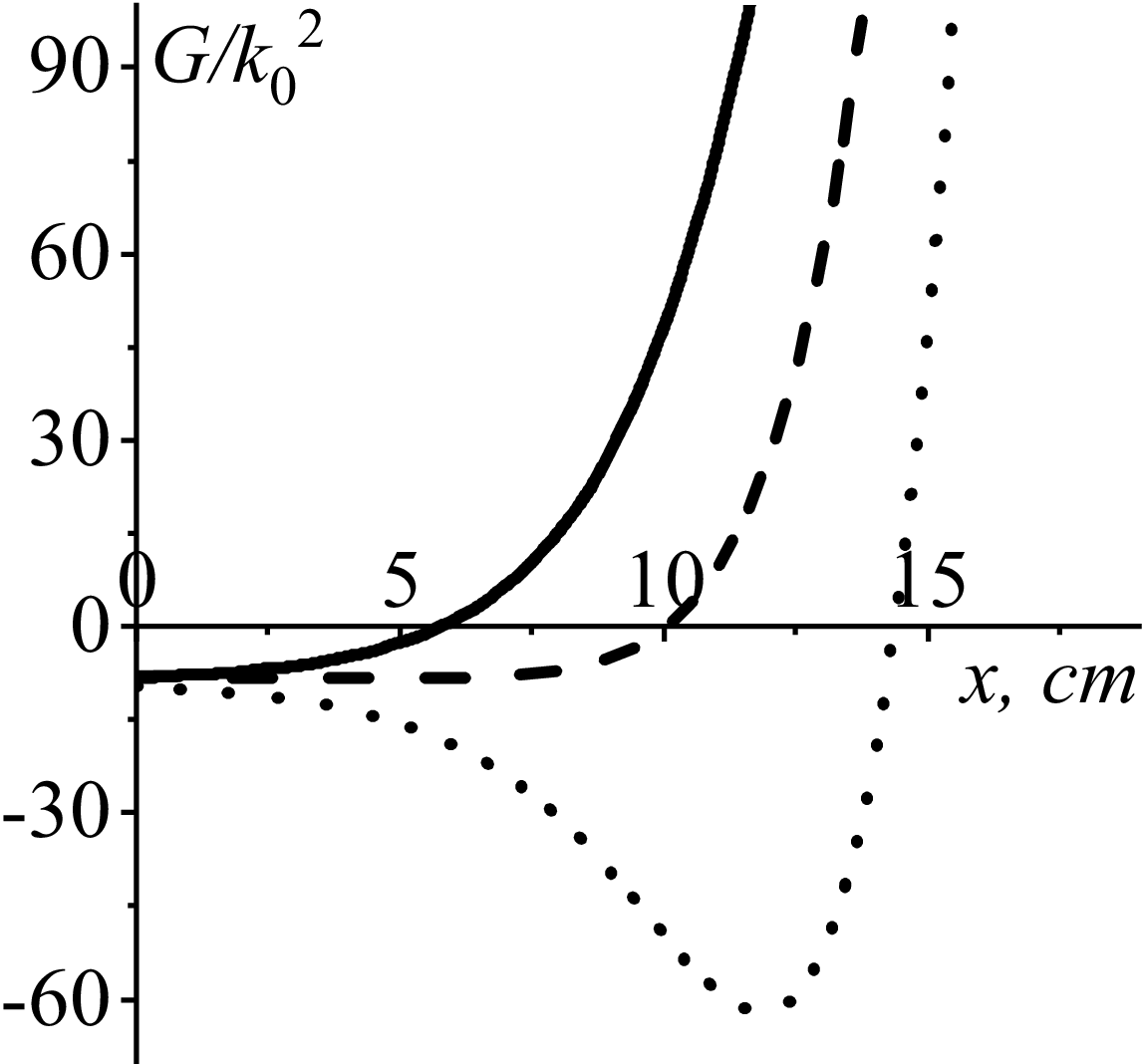
Figure 2 demonstrates evolution of the generalised perpendicular refractive index squared,
 $G(x)/{k}_{0}^{2}$
, for FMSWs with
 $N_{y}=-0.94$
(solid curve),
 $N_{y}=0.0$
(dashed curve),
 $N_{y}=+0.94$
(dotted curve). The following plasma and wave parameters are chosen:
 $N_{z}=3.0$
,
 $\varphi =2.687$
,
 $n(0)=10^{16}\,{\rm m}^{-3}$
,
 $\,\lambda =0.023\,{\rm cm}$
. Here, and hereinafter, plasma is assumed to consist of helium-3 ions and electrons. Cutoff positions are 5.77, 10.04 and
 $14.37\,{\rm cm}$
for FMSWs with
 $N_{y}=-0.94$
(solid curve),
 $N_{y}=0.0$
(dashed curve) and
 $N_{y}=+0.94$
(dotted curve), respectively. One can see from figure 2 that the spatial evolution of
 $G(x)$
is a far from linear one. This confirms the necessity of considering the three different regions mentioned above for searching the FMSW field spatial evolution if the evanescent layer is sufficiently wide.
Evolution of
 $G(x)/{k}_{0}^{2}$
for FMSWs with
 $N_{y}=-0.94$
(solid curve),
 $N_{y}=0.0$
(dashed curve),
 $N_{y}=+0.94$
(dotted curve). Here,
 $N_{z}=3.0$
,
 $\varphi =2.687$
,
 $n(0)=10^{16}\,{\rm m}^{-3}$
,
 $\,\lambda =0.023\,{\rm cm}$
.

5. Numerical analysis
To demonstrate the dependence of the fraction of the transmitted power,
 $P_{\textit{tran}}/P_{0}$
, on the plasma parameters: toroidal and poloidal refractive indices
 $N_{z}$
and
 $N_{y}$
, generator frequency
 $\varphi$
, plasma density decay length
 $\lambda$
and the plasma density at the antenna
 $n(0)$
, is the objective of the present numerical analysis. The basic plasma parameters are chosen from Messiaen & Maquet (Reference Messiaen and Maquet2020): in most cases the toroidal wave index
 $N_{z}=3.0$
and generator frequency
 $\varphi =2.687$
. Plasma density decay length
 $\lambda$
varies around
 $\lambda =0.02\,{\rm m}$
. The numerical analysis is carried out by means of the standard package ‘Wolfram Mathematica’, version 13.1 given in Wolfram (Reference Wolfram2022).
5.1. The dependence of the fraction of the transmitted power on the plasma density decay length
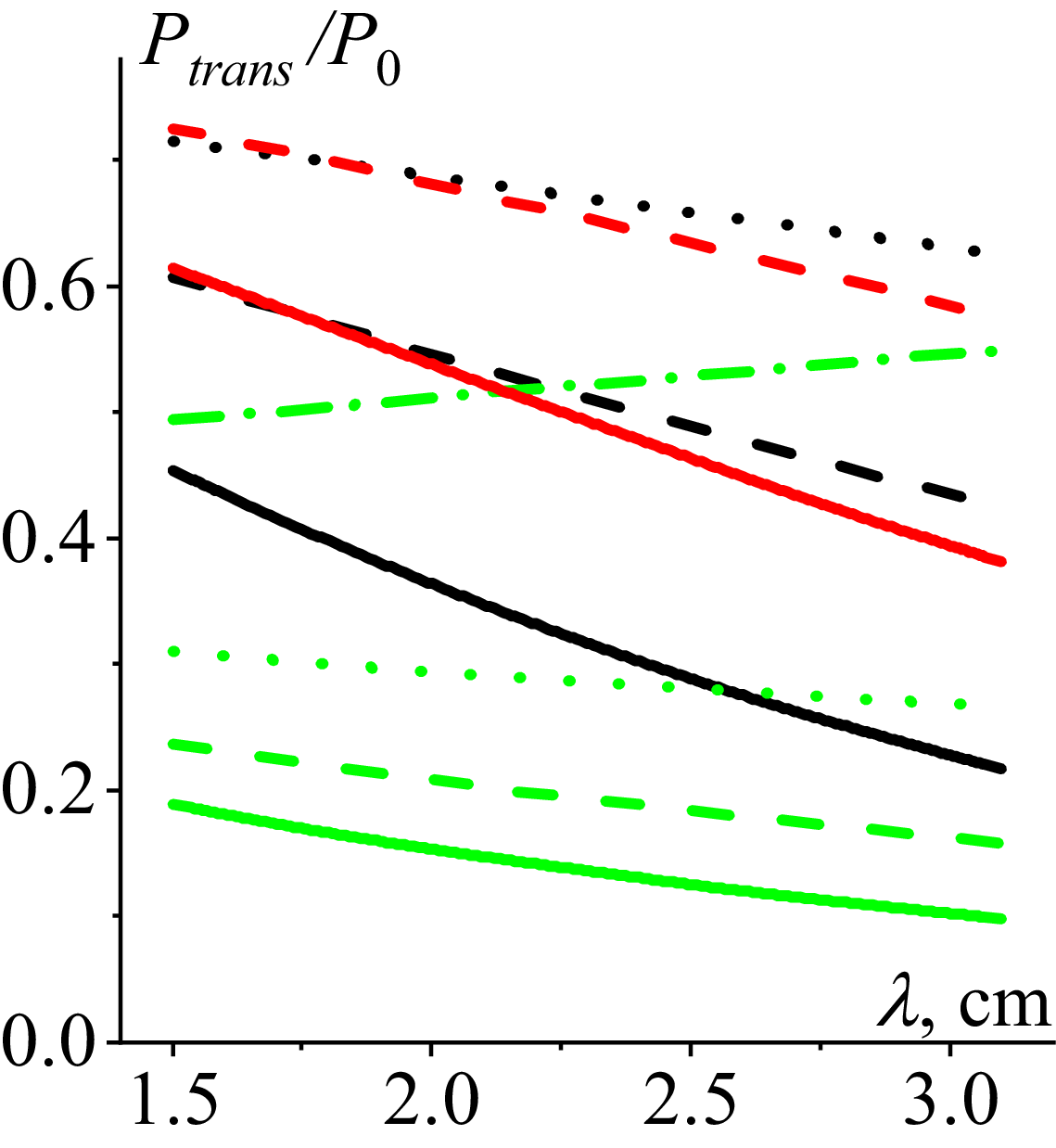
Figures 3–5 present the results of calculating
 $P_{\textit{tran}}/P_{0}$
for FMSWs with a positive poloidal refractive index
 $N_{y}=0.94$
(green curves), zero poloidal refractive index
 $N_{y}=0.0$
(black curves) and a negative poloidal refractive index
 $N_{y}=-094$
(red curves). In most of these figures, an increase of the plasma density decay length
 $\lambda$
causes a decrease of
 $P_{\textit{tran}}/P_{0}$
. For example, for the case of
 $N_{z}=3.0$
,
 $\varphi =2.67$
,
 $n(0)=10^{16}\,{\rm m}^{-3}$
,
 $\,N_{y}=-0.94$
(red dashed curve in figure 5) increase of the plasma density decay length from
 $\lambda =0.015\,{\rm }$
to
 $\lambda =0.031\,{\rm m}$
(by
 $\approx 2.1$
times) is accompanied by decrease of
 $P_{\textit{tran}}/P_{0}$
from
 $P_{\textit{tran}}/P_{0}=0.725$
to
 $P_{\textit{tran}}/P_{0}=0.574$
(by
 $\approx 1.3$
times).
The dependence of
 $P_{\textit{tran}}/P_{0}$
on
 $\,\lambda$
subject to toroidal refractive index:
 $N_{z}=3.0$
(solid curve),
 $\,\,N_{z}=5.0$
(dashed curve),
 $\,N_{z}=7.0$
(dotted curve),
 $N_{y}=0.94$
(green curves),
 $N_{y}=0$
(black curves),
 $N_{y}=-0.94$
(red curve). Here,
 $\varphi =2.687$
,
 $n(0)=10^{18}\,{\rm m}^{-3}$
.

The dependence of
 $P_{\textit{tran}}/P_{0}$
on
 $\,\lambda$
subject to the operating frequency:
 $\varphi =1.5$
(dashed curve),
 $\varphi =2.687$
(solid curve),
 $\varphi =4.5$
(dotted curve).
 $N_{y}=0.94$
(green curves),
 $N_{y}=0$
(black curves). Here,
 $N_{z}=3.0$
,
 $n(0)=10^{17}\,{\rm m}^{-3}$
.

The dependence of
 $P_{\textit{tran}}/P_{0}$
on
 $\,\lambda$
subject to the plasma density at the antenna:
 $n(0)=10^{15}\,{\rm m}^{-3}$
(solid curves),
 $n(0)=10^{16}\,{\rm m}^{-3}$
(dashed curves),
 $n(0)=10^{17}\,{\rm m}^{-3}$
(dotted curves),
 $n(0)=10^{18}\,{\rm m}^{-3}$
(dash-dotted curve),
 $N_{y}=0.94$
(green curves),
 $N_{y}=0$
(black curves),
 $N_{y}=-0.94$
(red curves). Here,
 $N_{z}=3.0$
,
 $\varphi =2.687$
.

Solid green curve in figure 3 and dash-dotted green curve in figure 5 are the only exceptions: they demonstrate an increase of
 $T(\eta _{0})$
(3.14) with an increase of
 $\lambda$
. These curves are calculated for the same set of plasma parameters:
 $N_{z}=3.0$
,
 $\varphi =2.687$
, positive poloidal refractive index
 $N_{y}=0.94$
and relatively high plasma density at the antenna
 $n(0)=10^{18}\,{\rm m}^{-3}$
. This qualitatively different dependence of the fraction of the transmitted power on
 $\lambda$
is explained in detail in Appendix D.
The dependence of
 $T(\eta _{0})$
on
 $\,\lambda$
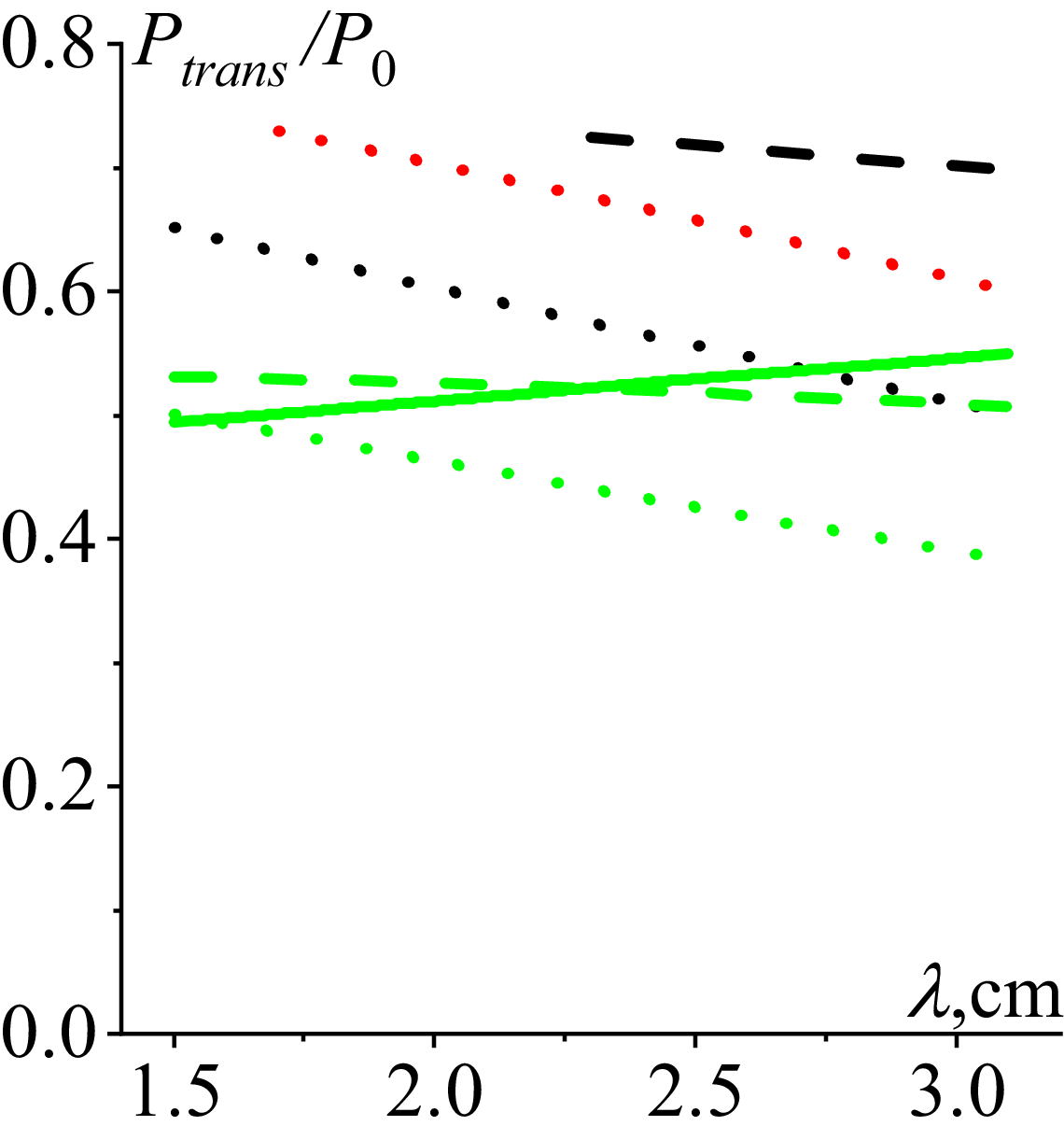
(in cm) subject to a toroidal refractive index is presented in figure 3. The following parameters of the plasma and wave are chosen for the calculations:
 $N_{z}=3.0$
(solid curve),
 $N_{z}=5.0$
(dashed curves),
 $\,N_{z}=7.0$
(dotted curves);
 $\varphi =2.67$
,
 $n(0)=10^{18}\,{\rm m}^{-3}$
. The curves related to FMSWs with
 $N_{y}=-0.94$
and toroidal refractive indices
 $N_{z}=3.0$
and
 $N_{z}=5.0$
are not shown in figure 3 since such FMSWs have no evanescent layer in front of the antenna for the chosen plasma parameters. The same is true for FMSWs with
 $N_{y}=0.0$
and
 $N_{z}=3.0$
. Black dashed curve related to FMSWs with
 $N_{y}=0.0$
and
 $N_{z}=5.0$
is displayed for
 $\lambda \geq 2.2\,{\rm cm}$
only since the evanescent layers are very thin for
 $\lambda \lt 2.2\,{\rm cm}$
so that applicability of Airy function asymptotes (3.7) fails. The applicability is checked by calculating the remainder term
 $5/(72\eta _{0})$
, which is chosen to be smaller than
 $0.9$
in the calculations within the present paper. These large values of the remainder term are observed when the curves in figures 3–5 approach the maximum of transmitted power,
 $Max\{T(\eta _{0})\}=0.8$
.
In all the cases, an increase of the toroidal wave index causes an increase of the evanescent layer width and depth, which in most cases results in the decrease of
 $P_{\textit{tran}}/P_{0}$
. Specifically, an increase of the toroidal refractive index from
 $N_{z}=5.0$
to
 $N_{z}=7.0$
(by
 $1.4$
times) for FMSWs with
 $N_{y}=0.0$
in the case of
 $\lambda =0.025\,{\rm m}$
is accompanied by a decrease of
 $P_{\textit{tran}}/P_{0}$
from
 $P_{\textit{tran}}/P_{0}=0.718$
to
 $P_{\textit{tran}}/P_{0}=0.556$
(by
 $\approx 1.3$
times). The evolution of the green solid curve in figure 3 is discussed in Appendix D.
The results presented in figure 3 are in qualitative agreement with the general principles of plasma electrodynamics. For a fixed radiated power, the larger the toroidal refractive index
 $| N_{z}|$
the wider and deeper the evanescence layer. After passing the wider and deeper evanescence layer, the wave power that reaches the cutoff decays by the factor
 $\exp (-2\eta _{0})$
. This decay causes decrease of the power transmitted through the cutoff, as well as decrease of the wave power reflected from the cutoff. This decrease is stronger for larger
 $| N_{z}|$
. After reflection from the cutoff, the reflected wave passes the evanescence layer once again, with a respective decrease of its power by the same factor
 $\exp (-2\eta _{0})$
. To summarise, an increase of
 $| N_{z}|$
is accompanied by a decrease of both transmitted and reflected wave power.
The dependence of
 $P_{\textit{tran}}/P_{0}$
on
 $\,\lambda$
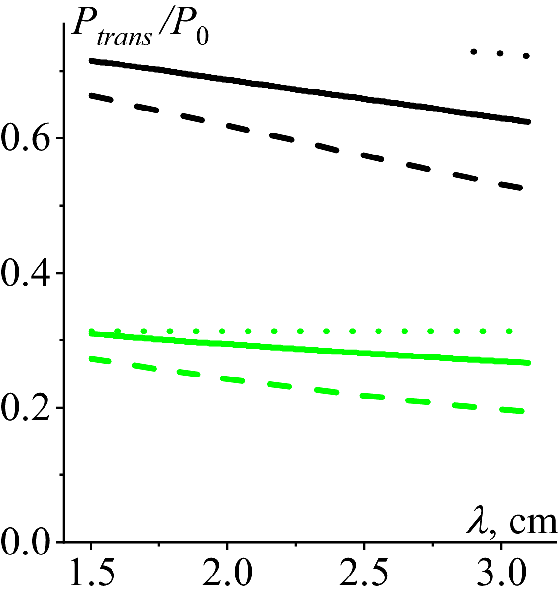
subject to the operating frequency is shown in figure 4. The following plasma and wave parameters are chosen:
 $\varphi =1.5$
(dashed curve),
 $\varphi =2.67$
(solid curve),
 $\varphi =4.5$
(dotted curve);
 $N_{z}=3.0$
,
 $n(0)=10^{17}\,{\rm m}^{-3}$
. No data related to FMSWs with negative refractive indices are displayed in figure 4 since they have no evanescent layer in front of the antenna for the chosen parameters. Dotted black curve related to FMSWs with
 $N_{y}=0$
is shown for
 $\lambda \geq 2.9\,{\rm cm}$
only since the evanescent layer becomes too small for
 $\lambda \lt 2.9\,{\rm cm}$
to provide applicability of Airy function asymptotes (3.7).
Increase of the operating frequency causes a decrease of evanescent layer width which in turn results in the increase of
 $P_{\textit{tran}}/P_{0}$
. For example, increase of the operating frequency from
 $\varphi =1.5$
to
 $\varphi =4.5$
(by three times) in the case of
 $\lambda =0.021\,{\rm m}$
is accompanied by increase of
 $P_{\textit{tran}}/P_{0}$
from
 $P_{\textit{tran}}/P_{0}=0.237$
to
 $P_{\textit{tran}}/P_{0}=0.313$
(by
 $\approx 32\%$
). The dependence of
 $P_{\textit{tran}}/P_{0}$
on
 $\,\lambda$
subject to the operating frequency is in qualitative agreement with that presented in figures 7 and 8 in Ram & Bers (Reference Ram and Bers1984).
The dependence of the fraction of the transmitted power on
 $\,\lambda$
subject to the plasma density at the antenna (
 $x=0$
) is demonstrated in figure 5. The following plasma and wave parameters are chosen:
 $n(0)=10^{15}\,{\rm m}^{-3}$
(solid curves),
 $n(0)=10^{16}\,{\rm m}^{-3}$
(dashed curves),
 $n(0)=10^{17}\,{\rm m}^{-3}$
(dotted curves),
 $n(0)=10^{18}\,{\rm m}^{-3}$
(dash-dotted curve);
 $N_{z}=3.0$
,
 $\varphi =2.687$
,
 $N_{y}=0.94$
(green curves),
 $N_{y}=0$
(black curves),
 $N_{y}=-0.94$
(red curves). The data concerning FMSWs with
 $N_{y}=-0.94$
for plasma densities at the antenna
 $n(0)=10^{17}\,{\rm m}^{-3}$
and
 $n(0)=10^{18}\,{\rm m}^{-3}$
are not shown in figure 5 since such FMSWs have no evanescent layer in front of the antenna. The same is true for FMSWs with
 $N_{y}=0$
for
 $n(0)=10^{18}\,{\rm m}^{-3}$
. Increase of the plasma density at the antenna causes a decrease of the evanescent layer width, which in turn results in the increase of
 $P_{\textit{tran}}/P_{0}$
. For instance, increase of the plasma density at the antenna from
 $n(0)=10^{15}\,{\rm m}^{-3}$
to
 $n(0)=10^{16}\,{\rm m}^{-3}$
in the case of
 $\lambda =0.021\,{\rm cm}$
is accompanied by increase of
 $P_{\textit{tran}}/P_{0}$
from
 $P_{\textit{tran}}/P_{0}=0.522$
to
 $P_{\textit{tran}}/P_{0}=0.672$
(by
 $\approx 29\%$
). The results presented in figure 5 are in qualitative agreement with those in Ram & Bers (Reference Ram and Bers1984), where the higher density at the edge was reported to lead to a higher reflection of the incident power.
Strong dependence of
 $P_{\textit{tran}}/P_{0}$
on the poloidal refractive index sign can be seen in figures 3–5. The coupling dependence on the poloidal wavenumber is well known (see, e.g. Ram & Bers Reference Ram and Bers1984). A detailed three-dimensional field analysis in a slab geometry for antenna–plasma coupling theory was presented therein. The calculated radiation impedance of a single antenna was shown to be significantly modified by including the finite poloidal length of the antenna. The plasma impedance was proved to be highly asymmetric in the poloidal refractive indices
 $N_{y}$
, with good coupling occurring for large negative values of
 $N_{y}$
. Strong sensitivity of the fraction of the transmitted power,
 $P_{\textit{tran}}/P_{0}$
, to the sign of the FMSW poloidal indices is confirmed in the present paper. The value of
 $P_{\textit{tran}}/P_{0}$
for FMSWs with positive
 $N_{y}$
is shown to be sufficiently smaller than those for FMSWs with zero and/or negative poloidal refractive indices, ceteris paribus. These results are also in agreement with those in Girka, Trush & Tierens (Reference Girka, Trush and Tierens2024). It was reported therein that the width of the evanescent layer (being different for different wave field components) for FMSWs with positive poloidal refractive indices is larger than that for FMSWs with zero and/or negative poloidal refractive indices. In most cases, the values of
 $P_{\textit{tran}}/P_{0}$
for FMSWs with
 $N_{y}=0.0$
(black curves) deviate less from those for FMSWs with negative poloidal refractive index
 $N_{y}=-0.94$
(red curves) then from those for FMSWs with positive poloidal refractive index
 $N_{y}=0.94$
(green curves).
The dependence of
 $\textrm{Re}(E_{y})$
on
 $x/\lambda : N_{y}=+0.94$
(solid curve),
 $N_{y}=0.0$
(dash-dotted curve),
 $\,N_{y}=-0.94$
(dashed curve). Here,
 $N_{z}=3.0$
,
 $\varphi =2.687$
,
 $n(0)=10^{15}\,{\rm m}^{-3}$
,
 $\,\lambda =1.7\,{\rm cm}$
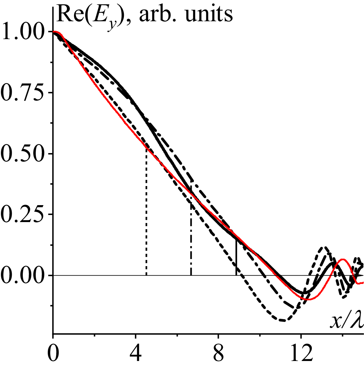
. Vertical lines indicate the positions of the corresponding cutoffs. The thin solid red curve is shown for comparison. This dependence of
 $\textrm{Re}(E_{y})$
on
 $x/\lambda$
is calculated numerically, taking into account the coupling between slow and fast waves for
 $N_{y}=0.0$
.

5.2. The wave field spatial evolution
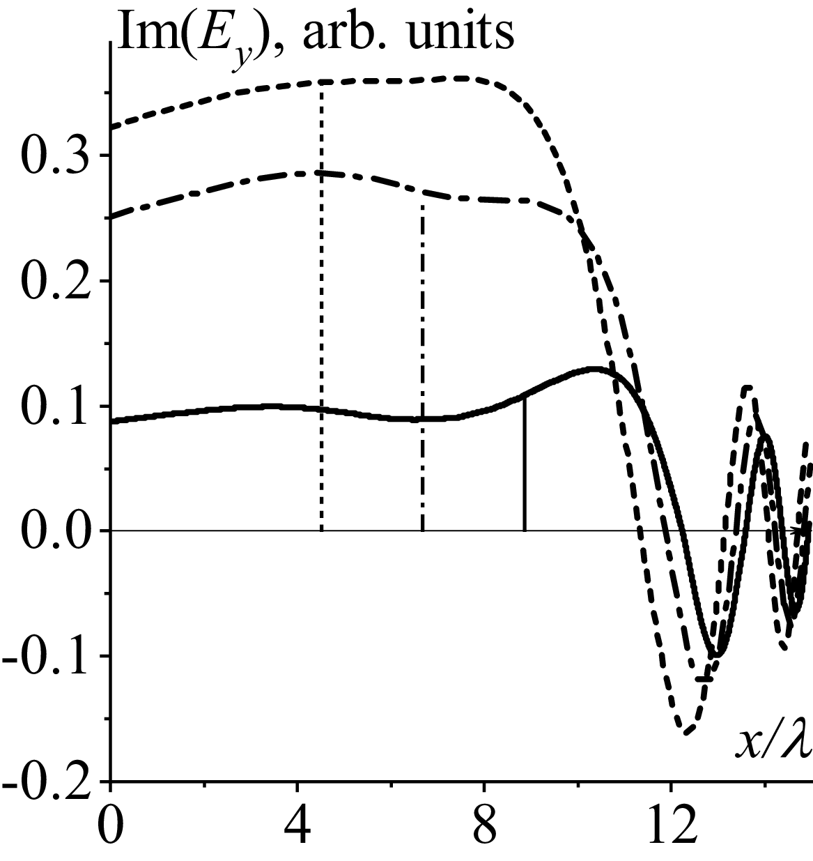
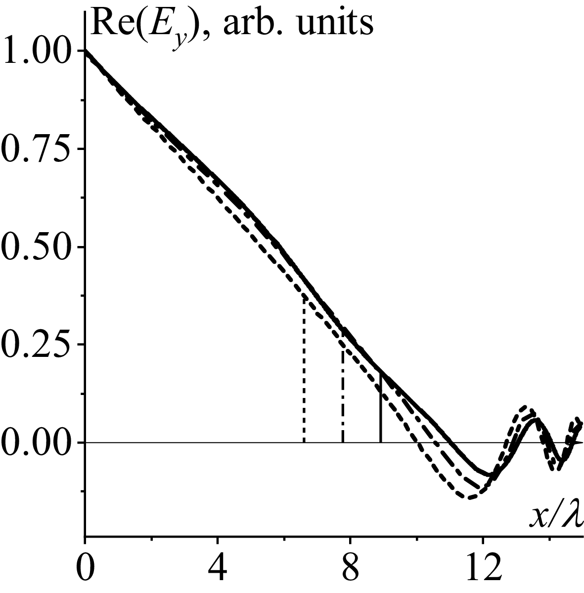
Spatial evolutions of the wave electric field
 $E_{y}$
amplitudes are presented in figures 6–9 for two toroidal refractive indices
 $N_{z}=3.0$
(see figures 6 and 7) and
 $N_{z}=5.0$
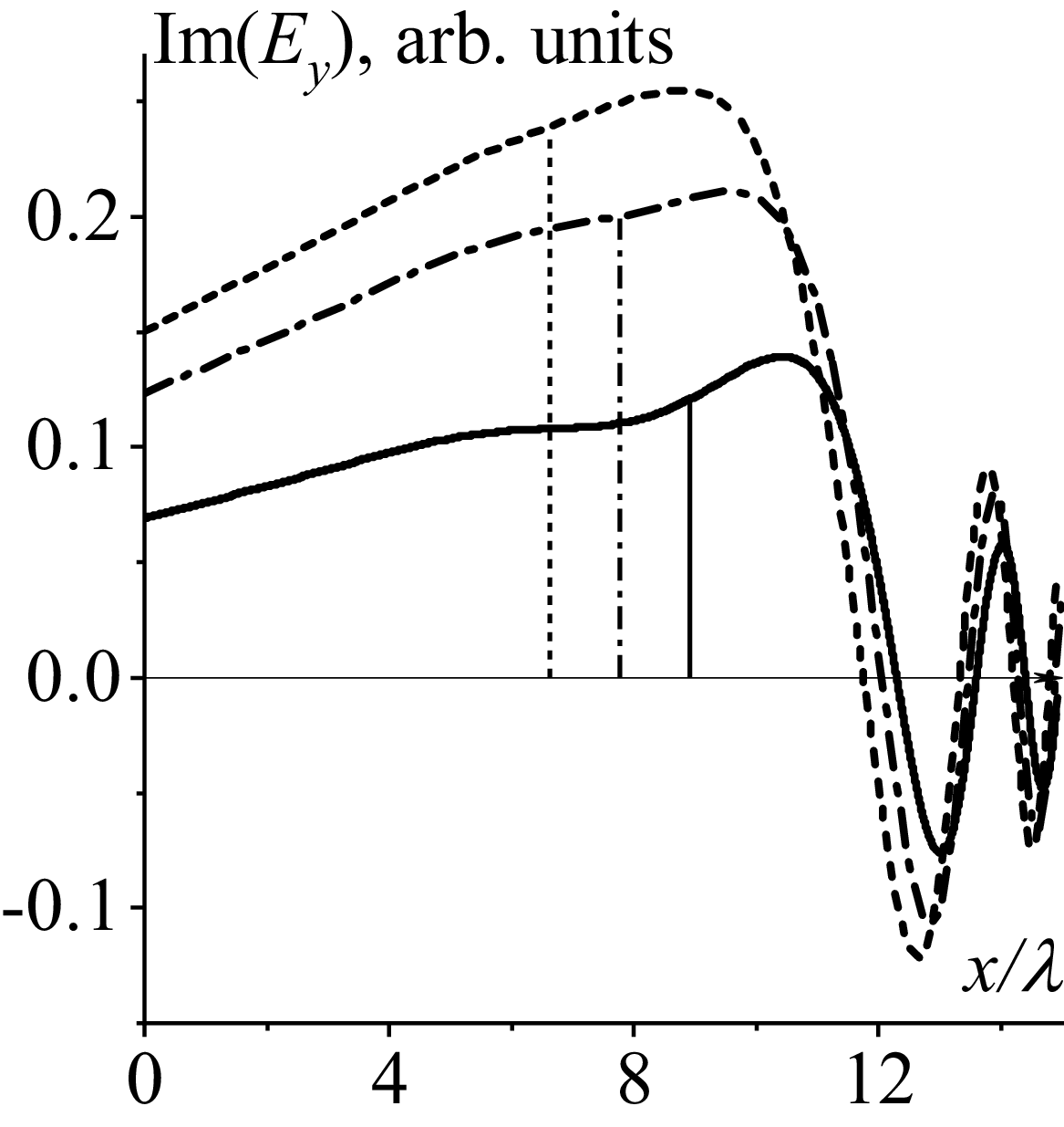
(see figures 8 and 9). Figures 6 and 8 relate to incident waves. Their amplitudes at the antenna are chosen to be unity. Figures 7 and 9 correspond to the reflected waves. The values of their amplitudes at the antenna agree with the calculations of the FMSW reflection coefficient. The curves related to positive poloidal refractive index
 $N_{y}=0.94$
are shown by solid curves. The curves corresponding to negative poloidal refractive index
 $N_{y}=-0.94$
are shown by dashed curves. Those calculated for zero poloidal refractive index
 $N_{y}=0.0$
are given by dash-dotted curves. Plasma density decay length is chosen as
 $\lambda =0.017\,{\rm cm}$
. The maximum value of
 $x$
in figures 6–9 approximately corresponds to the position of the last closed magnetic surface in figure 3 in Ragona & Messiaen (Reference Ragona and Messiaen2016). Operating frequency is chosen to be
 $\varphi =2.687$
, plasma density at the antenna is
 $n(0)=10^{15}\,{\rm m}^{-3}$
.
The dependence of
 $\text{Im}(E_{y})$
on
 $x/\lambda : N_{y}=+0.94$
(solid curve),
 $N_{y}=0.0$
(dash-dotted curve),
 $\,N_{y}=-0.94$
(dashed curve). Here,
 $N_{z}=3.0$
,
 $\varphi =2.687$
,
 $n(0)=10^{15}\,{\rm m}^{-3}$
,
 $\,\lambda =1.7\,{\rm cm}$
. Vertical lines indicate the positions of the corresponding cutoffs.

The same as in figure 6 but for
 $N_{z}=5.0$
. Vertical lines indicate the positions of the corresponding cutoffs.

The same as in figure 7 but for
 $N_{z}=5.0$
. Vertical lines indicate the positions of the corresponding cutoffs.

Vertical lines indicate the positions of the corresponding cutoffs of the
 $E_{y}$
wave field component: solid lines relate to the positions of the cutoff for FMSWs with positive poloidal refractive index
 $N_{y}=+0.94$
, dash-dotted lines relate to FMSWs with
 $N_{y}=0.0$
, and the dashed lines relate to the FMSWs with
 $\,N_{y}=-0.94$
. Specifically, the positions of cutoffs for FMSWs with toroidal refractive index
 $N_{z}=3.0$
in figures 6 and 7, are
 $x=0.1504\,{\rm m}$
for FMSWs with
 $N_{y}=+0.94$
(solid curve),
 $x=0.11\,{\rm m}$
for
 $N_{y}=0.0$
(dash-dotted curve) and
 $x=0.077\,{\rm m}$
for
 $\,N_{y}=-0.94$
(dashed curve). The evanescent layers are naturally wider for FMSWs with larger toroidal refractive indices. The cutoff positions for FMSWs with
 $N_{z}=5.0$
in figures 8 and 9 are located at
 $x=0.1516\,{\rm },\,0.13\,{\rm },\,0.11\,{\rm m}$
for FMSWs with
 $N_{y}=+0.94$
(solid curve),
 $N_{y}=0.0$
(dash-dotted curve) and
 $\,N_{y}=-0.94$
(dashed curve), respectively. Cutoffs for FMSWs with positive poloidal refractive index are the furthest from the antenna, which agrees with the results presented in figures 3–5 and in Girka et al. (Reference Girka, Trush and Tierens2024): their fractions of the transmitted power are the smallest. The evanescent layers for FMSWs with the negative refractive index are the narrowest, which agrees with the largest fractions of the transmitted power and amplitudes of the reflected wave at the antenna.
The thin solid red curve is shown in figure 6 for comparison. This dependence of
 $\textrm{Re}(E_{y})$
on
 $x/\lambda$
is calculated numerically, taking into account the coupling between slow and fast waves (from the full fourth-order cold plasma wave equation) for
 $N_{y}=0.0$
. The comparison of the thin solid red curve with the dash-dotted curve calculated based on asymptotic expressions (2.5)–(2.9) (from truncated second-order (2.2)) demonstrates sufficient qualitative agreement.
When preparing the data for figures 3–9 the presence of the first region is checked by calculating the ratio of the spatial scale of the wave to that of plasma non-uniformity (the observable
 $| ({1}/{G^{1.5}})({{\rm d}G}/{{\rm d}x})|$
) which smallness justifies application of the WKB approximation. The calculations confirm the presence of the first region at least in an unneglectable part of the evanescent layer near the antenna for the cases considered in the present paper. It is clear that, for other plasma parameters, e.g. for higher plasma density in front of the antenna, the evanescent layer is narrower and the conditions for considering the first region fail. In this case, the results obtained in the present paper (in particular, (3.14)) remain valid until the asymptotic representations (3.7) of Airy functions are applicable. One can apply the asymptotes if the arguments of Airy functions at the antenna
 $\xi (0)=\big(({3}/{2}){\int }_{\kern-2pt 0}^{d}\sqrt{-G}{\rm d}x\big)^{2/3}$
are sufficiently large to neglect the next term in the series. The latter condition reads
 $\eta _{0}={\int }_{\kern-2pt 0}^{d}\sqrt{-G}{\rm d}x\gg 5/72\approx 0.07$
(see pages 448 and 449 in Abramowitz & Stegun (Reference Abramowitz and Stegun1964) for details).
6. Conclusions
The present paper develops an analytical approach to studying the influence of an evanescence layer in front of an antenna on the fraction of the transmitted power,
 $P_{\textit{tran}}/P_{0}$
, of the FMSWs presented in Bilato et al. (Reference Bilato, Brambilla, Hartmann and Parisot2005) by accounting for possible non-zero poloidal wave indices of FMSWs. The dependencies of
 $P_{\textit{tran}}/P_{0}$
on the plasma density decay length
 $\lambda$
subject to toroidal and poloidal refractive indices, operating frequency and plasma density in front of the antenna are presented.
The key conclusion of Bilato et al. (Reference Bilato, Brambilla, Hartmann and Parisot2005) was that the exponential factor
 $exp(-2| k_{z}| d)$
, commonly applied for the description of an evanescent layer in front of ion cyclotron fast-wave antennas effect on coupling was too pessimistic. The present analysis confirms this conclusion in calculations for FMSWs with zero poloidal refractive index (
 $N_{y}=0$
),
 ${\int }_{0}^{d}\kappa _{\bot }{\rm d}x\lt | k_{z}| d$
. However, the calculations related to FMSWs with positive poloidal refractive indices,
 $N_{y}\gt 0$
, show that
 ${\int }_{0}^{d}\sqrt{-G}{\rm d}x\gt | k_{z}| d$
. The inequality
 ${\int }_{0}^{d}\sqrt{-G}{\rm d}x\gt | k_{z}| d$
is also recorded in some calculations related to FMSWs with sufficiently large negative poloidal refractive indices,
 $N_{y}\lt 0$
. For example, the inequality
 ${\int }_{0}^{d}\sqrt{-G}{\rm d}x\gt | k_{z}| d$
is observed in the calculations for FMSWs with
 $N_{y}=-1.88$
,
 $\varphi =1.5$
,
 $N_{z}=3.0$
,
 $n(0)=10^{15}\,{\rm m}^{-3}$
if the plasma density decay length
 $\lambda \geq 1.66\,{\rm cm}$
.
Increase of the plasma density decay length
 $\lambda$
, ceteris paribus, is accompanied by a widening of the evanescent layer:
 $P_{\textit{tran}}/P_{0}$
decreases with an increase of
 $\lambda$
in most cases. The FMSWs with positive poloidal refractive indices
 $N_{y}$
appear to be less sensitive to the variation of
 $\lambda$
compared with FMSWs with zero and negative
 $N_{y}$
.
The present study confirms the conclusion reported in Ram & Bers (Reference Ram and Bers1984) about better coupling of FMSWs with negative poloidal refractive indices
 $N_{y}$
than of those with positive
 $N_{y}$
. This should be taken into account in designing and phasing future antennae in ion cyclotron range of frequencies (ICRF).
The present paper develops the theory of ICRF power transmission from an antenna to the core plasma, analysing the influence of a non-zero poloidal wave index and the plasma density decay length on the transmitted power. The model is an extension of that presented in Bilato et al. (Reference Bilato, Brambilla, Hartmann and Parisot2005) and is intentionally kept analytically tractable; as a consequence, several physically significant effects have been left aside. Among these are the confluence of fast and slow waves, the complex toroidal geometry of a tokamak and three-dimensional non-uniformities of both the plasma density and the equilibrium magnetic field. A particular consequence of neglecting wave coupling is worth noting: within the decoupled fast-wave model, the field components exhibit a singular behaviour at the layer
 ${S=N}_{z}^{2}$
, which is simultaneously the Alfvén resonance of the isolated fast wave and the cutoff of the slow wave. Once the coupling between the two waves is retained, this singularity is resolved and the layer becomes a mode-conversion region, potentially modifying the spatial evolution of the fast wave and the transmitted power. A systematic treatment of these effects is beyond the scope of the present paper and is likely to require only numerical tools beyond a reduced analytical model.
Furthermore, the wave evolution in front of the ICRF antenna is the result of interference between sets of modes propagating away from and towards the antenna. Numerous wave phenomena – confluences, mode conversion, the excitation of surface waves on steep gradients and a number of other processes that cannot be accounted for within the framework of the reduced equation (4.1) – can affect incident and reflected waves in different ways. The combination of modes that grow and decay exponentially, together with the presence of peaks in the wave equation caused by cutoffs and/or resonances, may result in the solutions being sensitive to specific plasma parameters.
The assumption of plasma density exponential decay applied in the present paper is based on Stangeby (Reference Stangeby2000) as well as experimental plasma density measurements (see, e.g. Paulus et al. Reference Paulus2025). This plasma density evolution (2.1) is applied for numerical analysis. The assumption of the plasma density exponential decay is of significance also for applying Bessel functions of the first kind of the zeroth order for searching the asymptotic solution of Maxwell’s equations (2.2) and (4.1) in the third region (sufficiently far from the cutoff in the transparent plasma of a tokamak scrape off layer). However, this assumption cannot be considered as a significant restriction for the obtained results. Assumption about the absence of the radio frequency power reflection from a dense plasma provides the relation between two linearly independent solutions of Airy type in (3.6), and the latter relation results in the dependence (3.14) of the transmission coefficient on the optical thickness
 $T(\eta _{0})$
which is the crucial point for further numerical analysis in the present paper.
Acknowledgements
One of the authors is very thankful to the Ukrainian Armed Forces for being alive. He is also grateful to the German people, and in particular to MPIPP, for the chance to work in Garching. The authors are thankful to the reviewers for their helpful comments.
Editor Paolo Ricci thanks the referees for their advice in evaluating this article.
Declaration of interests
The authors report no conflict of interest.
Appendix A. Derivation of asymptotic expressions for the wave field amplitudes in the first region
Theoretical fundamentals of asymptotic methods for solving differential equations are presented in particular in Fedoryuk (Reference Fedoryuk1993). The plasma density in the first region is assumed to be sufficiently small such that
 ${N}_{\bot }^{2}$
(see (1.1)) is negative and almost uniform. It is in place to emphasise that steep gradients of the plasma density (2.1) do not necessarily imply a sharp change in the refractive index
 ${N}_{\bot }^{2}$
if the plasma density is sufficiently small. Under these conditions, (2.2) has the form of an ordinary homogeneous second-order differential equation with constant coefficients,
 ${k}_{\bot }^{2}=-{k}_{\bot 0}^{2}$
. Solution of this equation is well known to be expressed in terms of exponential functions
 \begin{align}E_{y}=A_{01}\exp (-k_{\bot 0}x)+A_{02}\exp (k_{\bot 0}x).\end{align}
According to the theory mentioned above, exponential functions are chosen as the reference ones, and the spatial evolution of
 ${k}_{\bot }^{2}(x)$
is taken into account in two ways. First, the constants are assumed to vary weakly,
 $A_{01,02}\rightarrow A_{1,2}(x)$
, and second, deviation of the arguments of exponential functions from linearity is expected,
 $k_{\bot 0}x\rightarrow \,\chi (x)$
 \begin{align}E_{y}=A_{1}(x)\exp (-\chi (x))+A_{2}(x)\exp (\chi (x)),\end{align}
 \begin{align}\frac{d\kern-1.5pt E_{y}}{{\rm d}x}=\frac{d\kern-1.4pt A_{1}}{{\rm d}x}\exp (-\chi)+\frac{d\kern-1.4pt A_{2}}{{\rm d}x}\exp (\chi)-A_{1}\frac{d\kern-1pt \chi }{{\rm d}x}\exp (-\chi)+A_{2}\frac{d\kern-1pt \chi }{{\rm d}x}\exp (\chi),\end{align}
 \begin{align}\frac{d^{2}E_{y}}{{\rm d}x^{2}} & =\frac{d^{2}A_{1}}{{\rm d}x^{2}}\exp (-\chi)+\frac{d^{2}A_{2}}{{\rm d}x^{2}}\exp (\chi)-2\frac{d\kern-1.4pt A_{1}}{{\rm d}x}\frac{d\kern-1pt \chi }{{\rm d}x}\exp (-\chi)+2\frac{d\kern-1.4pt A_{2}}{{\rm d}x}\frac{d\kern-1pt \chi }{{\rm d}x}\exp (\chi)\nonumber\\[5pt]& \quad + A_{1}\!\left(\frac{d\kern-1pt \chi }{{\rm d}x}\right)^{2}\exp (-\chi)+A_{2}\!\left(\frac{d\kern-1pt \chi }{{\rm d}x}\right)^{2}\exp (\chi)-A_{1}\frac{d^{2}\chi }{{\rm d}x^{2}}\exp (-\chi)+A_{2}\frac{d^{2}\chi }{{\rm d}x^{2}}\exp (\chi).\end{align}
The terms proportional to
 $\exp (\pm \chi )$
are singled out in the rhs of (A4)
 \begin{align}\frac{d^{2}E_{y}}{{\rm d}x^{2}} & =\exp (-\chi)\left[\frac{d^{2}A_{1}}{{\rm d}x^{2}}-2\frac{d\kern-1.4pt A_{1}}{{\rm d}x}\frac{d\kern-1pt \chi }{{\rm d}x}+A_{1}\left(\frac{d\kern-1pt \chi }{{\rm d}x}\right)^{2}-A_{1}\frac{d^{2}\chi }{{\rm d}x^{2}}\right]\nonumber\\[5pt]& \quad +\exp (\chi)\left[\frac{d^{2}A_{2}}{{\rm d}x^{2}}+2\frac{d\kern-1.4pt A_{2}}{{\rm d}x}\frac{d\kern-1pt \chi }{{\rm d}x}+A_{2}\left(\frac{d\kern-1pt \chi }{{\rm d}x}\right)^{2}+A_{2}\frac{d^{2}\chi }{{\rm d}x^{2}}\right].\end{align}
Substitution of expressions (A2) and (A5) into (2.2) provides the following:
 \begin{align} & \exp (-\chi)\left[\frac{d^{2}A_{1}}{{\rm d}x^{2}}-2\frac{d\kern-1.4pt A_{1}}{{\rm d}x}\frac{d\kern-1pt \chi }{{\rm d}x}+A_{1}\left(\frac{d\kern-1pt \chi }{{\rm d}x}\right)^{2}-A_{1}\frac{d^{2}\chi }{{\rm d}x^{2}}+A_{1}{k}_{\bot }^{2}\right]\nonumber\\[5pt]& \quad+\exp (\chi)\left[\frac{d^{2}A_{2}}{{\rm d}x^{2}}+2\frac{d\kern-1.4pt A_{2}}{{\rm d}x}\frac{d\kern-1pt \chi }{{\rm d}x}+A_{2}\left(\frac{d\kern-1pt \chi }{{\rm d}x}\right)^{2}+A_{2}\frac{d^{2}\chi }{{\rm d}x^{2}}+A_{2}{k}_{\bot }^{2}\right]=0.\end{align}
To satisfy (A6) both factors by
 $\exp (\pm \chi )$
should be equal to zero. Let us consider the factor
 $\exp (\chi )$
. The term
 $({d^{2}A_{2}})/({{\rm d}x^{2}})$
is neglected since an exponential function is more sensitive to changes of its argument. The other four terms are distributed into two groups
 \begin{align}A_{2}\left(\frac{d\kern-1pt \chi }{{\rm d}x}\right)^{2}+A_{2}{k}_{\bot }^{2}=0,\end{align}
 \begin{align}2\frac{d\kern-1.4pt A_{2}}{{\rm d}x}\frac{d\kern-1pt \chi }{{\rm d}x}+A_{2}\frac{d^{2}\chi }{{\rm d}x^{2}}=0.\end{align}
To satisfy (A7), the argument of exponential functions reads
 \begin{align}\chi (x)=\pm {\int }_{\kern-4pt 0}^{x}\sqrt{-{k}_{\bot }^{2}}{\rm d}x.\end{align}
After precise dependence
 $\chi (x)$
is known, the dependence of amplitude
 $A_{2}(x)$
can be derived from (A8)
 \begin{align}A_{2}(x)\propto {\kappa _{\bot }}^{-1/2}.\end{align}
The result (A10) does not depend on the sign of the right-hand side of (A9).
The factor
 $\exp (-\chi )$
in (A6) should also be equal to zero. The term
 $({d^{2}A_{1}})/({{\rm d}x^{2}})$
is neglected for the same reason as it is above in regard to the term
 $({d^{2}A_{2}})/({{\rm d}x^{2}})$
. The other four terms in square brackets for
 $\exp (-\chi )$
in (A6) are split into two groups, which follow from (A7) and (A8) by only replacing the subscript
 $2$
by
 $1 : A_{2}\rightarrow A_{1}$
. The replacement does not change the expression (A9) for the argument
 $\chi (x)$
, and saves the dependence (A10) for the amplitude
 \begin{align}A_{1}(x)\propto {\kappa _{\bot }}^{-1/2}.\end{align}
Finally, substituting the definitions (A9), (A10) and (A11) into (A2) makes it possible to write down the asymptotic expression for the wave electric field amplitude in the form (2.5).
Appendix B. Derivation of asymptotic expressions for the wave field amplitudes in the second region
The presence of a cutoff,
 ${k}_{\bot }^{2}=0$
, at
 $x=d$
is the characteristic feature of the second region. This makes it possible to write down (2.2) in truncated representation
 \begin{align}\frac{{d^{2}}E_{y}}{{\rm d}x^{2}}+\frac{{dk}_{\bot }^{2}}{{\rm d}x}_{| x=d}(x-d)\,E_{y}=0.\end{align}
Equation (B1) is the well-known Airy equation (see page 446 in Abramowitz & Stegun Reference Abramowitz and Stegun1964). Airy functions
 $\mathrm{Ai}(\xi )$
and
 $\mathrm{Bi}(\xi )$
are two linearly independent solutions of (B1). That is why the general solution of (B1) can be written as
 \begin{align}E_{y}=B_{01}\mathrm{Ai}\left(-\left(\frac{{dk}_{\bot }^{2}}{{\rm d}x}_{| x=d}\right)^{{1}/{3}}(x-d)\right)+B_{02}\mathrm{Bi}\left(-\left(\frac{{dk}_{\bot }^{2}}{{\rm d}x}_{| x=d}\right)^{{1}/{3}}(x-d)\right).\end{align}
Deviation of
 ${k}_{\bot }^{2}(x)$
from linearity is taken into account in two ways following the theory of asymptotic solving the ordinary differential equations described e.g. in Fedoryuk (Reference Fedoryuk1993). First, the constants are assumed to vary weakly,
 $B_{01,02}\rightarrow B_{1,2}(x)$
, and second, deviation of the arguments of Airy functions from linearity is expected,
 $\big(-\big(({{dk}_{\bot }^{2}})/({{\rm d}x}_{| x=d})\big)^{{1}/{3}}(x-d)\big)\rightarrow \,\xi (x)$
. In other words, asymptotic solution of (2.2) in the second region is to be found in the following form:
 \begin{align}{E}_{y}^{(2)}=B_{1}(x)\mathrm{Ai}(\xi (x))+B_{2}(x)\mathrm{Bi}(\xi (x)).\end{align}
Then the second derivative
 $({d^{2}{E}_{y}^{(2)}})/({{\rm d}x^{2}})$
reads
 \begin{align}\frac{d^{2}{E}_{y}^{(2)}}{{\rm d}x^{2}} & =\frac{d^{2}B_{1}}{{\rm d}x^{2}}\mathrm{Ai}(\xi)+\frac{d^{2}B_{2}}{{\rm d}x^{2}}\mathrm{Bi}(\xi)+2\frac{dB_{1}}{{\rm d}x}\frac{d\mathrm{Ai}}{{\rm d}\xi }\frac{{\rm d}\xi }{{\rm d}x}+2\frac{dB_{2}}{{\rm d}x}\frac{d\mathrm{Bi}}{{\rm d}\xi }\frac{{\rm d}\xi }{{\rm d}x}\nonumber\\[10pt]& \quad + B_{1}\frac{d^{2}\mathrm{Ai}}{{\rm d}\xi ^{2}}\left(\frac{{\rm d}\xi }{{\rm d}x}\right)^{2}+B_{2}\frac{d^{2}\mathrm{Bi}}{{\rm d}\xi ^{2}}\left(\frac{{\rm d}\xi }{{\rm d}x}\right)^{2}+B_{1}(x)\frac{d\mathrm{Ai}}{{\rm d}\xi }\frac{d^{2}\xi }{{\rm d}x^{2}}+B_{2}(x)\frac{d\mathrm{Bi}}{{\rm d}\xi }\frac{d^{2}\xi }{{\rm d}x^{2}},\end{align}
Substituting the result (B4) into (2.2) provides
 \begin{align}& \frac{d^{2}B_{1}}{{\rm d}x^{2}}\mathrm{Ai} +2\frac{dB_{1}}{{\rm d}x}\frac{d\mathrm{Ai}}{{\rm d}\xi }\frac{{\rm d}\xi }{{\rm d}x}+B_{1}\frac{d^{2}\mathrm{Ai}}{{\rm d}\xi ^{2}}\left(\frac{{\rm d}\xi }{{\rm d}x}\right)^{2}+B_{1}\frac{d\mathrm{Ai}}{{\rm d}\xi }\frac{d^{2}\xi }{{\rm d}x^{2}}+{k}_{\bot }^{2}B_{1}\mathrm{Ai}\nonumber\\[5pt]& \quad +\frac{d^{2}B_{2}}{{\rm d}x^{2}}\mathrm{Bi}+2\frac{dB_{2}}{{\rm d}x}\frac{d\mathrm{Bi}}{{\rm d}\xi }\frac{{\rm d}\xi }{{\rm d}x}+B_{2}\frac{d^{2}\mathrm{Bi}}{{\rm d}\xi ^{2}}\left(\frac{{\rm d}\xi }{{\rm d}x}\right)^{2}\!+B_{2}\frac{d\mathrm{Bi}}{{\rm d}\xi }\frac{d^{2}\xi }{{\rm d}x^{2}}+{k}_{\bot }^{2}B_{2}\mathrm{Bi}=0.\end{align}
Second derivatives of Airy functions in respect of their arguments should be replaced according to the definition of Airy functions
 \begin{align}\frac{d^{2}\mathrm{Ai}}{{\rm d}\xi ^{2}}=\xi \mathrm{Ai}(\xi), \quad \frac{d^{2}\mathrm{Bi}}{{\rm d}\xi ^{2}}=\xi \mathrm{Bi}(\xi).\end{align}
Two groups of terms in (B5), those containing
 $\mathrm{Ai}(\xi )$
and its first derivative
 $({d\mathrm{Ai}})/({{\rm d}\xi })$
, and those proportional to
 $\mathrm{Bi}(\xi )$
and its first derivative
 $({d\mathrm{Bi}})/({{\rm d}\xi })$
, should be equal to zero independently.
In the following, the first group is considered in detail. The term
 $({d^{2}B_{1}})/({{\rm d}x^{2}})\mathrm{Ai}$
is neglected since Airy functions are more sensitive to the change of their arguments
 \begin{align}\left| \frac{d^{2}B_{1}}{{\rm d}x^{2}}\mathrm{Ai}\right| \ll \left| 2\frac{dB_{1}}{{\rm d}x}\frac{d\mathrm{Ai}}{{\rm d}\xi }\frac{{\rm d}\xi }{{\rm d}x}\right|.\end{align}
The expression (B3) contains two unknown variables to be determined. That is why the other four terms in (B5) proportional to
 $\mathrm{Ai}(\xi )$
and its first derivative
 $(({d\mathrm{Ai}})/{{\rm d}\xi })$
are used to form two first-order differential equations
 \begin{align}\left(\xi \left(\frac{{\rm d}\xi }{{\rm d}x}\right)^{2}+{k}_{\bot }^{2}\right)B_{1}\mathrm{Ai}(\xi)=0,\end{align}
 \begin{align}\left(2\frac{dB_{1}}{{\rm d}x}\frac{{\rm d}\xi }{{\rm d}x}+B_{1}\frac{d^{2}\xi }{{\rm d}x^{2}}\right)\frac{d\mathrm{Ai}}{{\rm d}\xi }=0.\end{align}
Equation (B8) is used to determine the Airy function argument
 \begin{align}\xi (x)=\begin{cases} \xi (x)=\left(-\dfrac{3}{2}{\displaystyle\int }_{\kern-2pt d}^{x}\sqrt{{-k}_{\bot }^{2}}{\rm d}x\right)^{2/3},\,i\kern-2pt f\,x\lt d;\\[15pt] \xi (x)=-\left(\dfrac{3}{2}{\displaystyle\int }_{\kern-2pt d}^{x}\sqrt{{k}_{\bot }^{2}}{\rm d}x\right)^{{2}/{3}},\,i\kern-2pt f\,x\gt d. \end{cases}\end{align}
After the Airy function argument is determined one can derive the dependence of the amplitude
 $B_{1}(x)$
from (B9)
 \begin{align}B_{1}(x)\propto \left(-\frac{{\rm d}\xi }{{\rm d}x}\right)^{-({1}/{2})}.\end{align}
The same procedure as carried out in the present appendix for the terms containing
 $\mathrm{Ai}(\xi )$
and its first derivative
 $d\mathrm{Ai}/{\rm d}\xi$
can be repeated for those proportional to
 $\mathrm{Bi}(\xi )$
and its first derivative
 $d\mathrm{Bi}/{\rm d}\xi$
. It naturally provides the definition (B10) for Airy function argument, and a dependence like (B11) for the amplitude
 $A_{1}(x)$
 \begin{align}A_{1}(x)\propto \left(-{\rm d}\xi /{\rm d}x\right)^{-({1}/{2})}.\end{align}
Finally, substituting the results (B10), (B11) and (B12) into (B3) gives the asymptotic expression for the wave electric field amplitude in the second region in the form of (2.6).
Appendix C. Derivation of asymptotic expressions for the wave field amplitudes in the third region
In the third region, sufficiently far from the cutoff,
 ${k}_{\bot }^{2}$
increases approximately proportionally to the plasma density
 \begin{align}{k}_{\bot }^{2}\approx k_{\bot }^{2}(d)\exp [(x-d)/\lambda ].\end{align}
Then (2.2) reads
 \begin{align}\frac{{d^{2}}E_{y}}{{\rm d}x^{2}}+{k}_{\bot }^{2}(d)\exp \left[\frac{x-d}{\lambda }\right]E_{y}=0.\end{align}
The following algebra transforms (C2) to the zero-order Bessel equation. First, (C2) is divided by exponential factor
 $\exp \left[{(x-d)}/{\lambda }\right]$
 \begin{align}\frac{1}{\exp [({x-d})/{2\lambda }]}\frac{1}{\exp [({x-d})/({2\lambda })]}\frac{\rm d}{{\rm d}x}\left(\frac{\exp \left[({x-d})/({2\lambda })\right]}{\exp \left[({x-d})/({2\lambda })\right]}\frac{d\kern-1.5pt E_{y}}{{\rm d}x}\right)+{k}_{\bot }^{2}(d)E_{y}=0.\end{align}
Second, the variable is replaced,
 $k_{\bot }(d)\exp [({x-d})/({2\lambda })]{\rm d}x=2k_{\bot }(d)\lambda d$
 $(\exp [({x-d})/({2\lambda })])=d\phi$
 \begin{align}\frac{1}{\phi }\frac{\rm d}{\rm d\phi }\left(\phi \frac{{d}E_{y}}{{\rm d}\phi }\right)+E_{y}=0.\end{align}
Solution of (C4) can be represented in terms of zero-order Bessel functions of the first,
 $J_{0}(\phi )$
, and second,
 $Y_{0}(\phi )$
, kinds (see page 358 in Abramowitz & Stegun Reference Abramowitz and Stegun1964)
 \begin{align}E_{y}=C_{01}J_{0}(\phi)+C_{02}Y_{0}(\phi).\end{align}
Deviation of
 ${k}_{\bot }^{2}(x)$
from exponential evolution (C1) is taken into account in two ways. First, the spatial dependence of Bessel function argument is permitted to be different from the exponential one,
 $\phi \rightarrow p(x)$
. Second, factors
 $C_{01}$
and
 $C_{02}$
are expected to be found weakly dependent on
 $x$
,
 $C_{01,02}\rightarrow C_{1,2}(x)$
. This makes it possible to search the wave electric field amplitude in this region in the following asymptotic form:
 \begin{align}{E}_{y}^{(3)}=C_{1}(x)J_{0}(p(x))+C_{2}(x)Y_{0}(p(x)).\end{align}
Then the second derivative
 $({{d^{2}E}_{y}^{(3)}})/({{\rm d}x^{2}})$
reads
 \begin{align}\frac{{d^{2}E}_{y}^{(3)}}{{\rm d}x^{2}} & =\frac{d^{2}C_{1}}{{\rm d}x^{2}}J_{0}+\frac{d^{2}C_{2}}{{\rm d}x^{2}}Y_{0}+2\frac{dC_{1}}{{\rm d}x}\frac{d\kern-1.1pt J_{0}}{dp}\frac{dp}{{\rm d}x}+2\frac{dC_{2}}{{\rm d}x}\frac{dY_{0}}{dp}\frac{dp}{{\rm d}x}\nonumber\\[5pt]& \quad + C_{1}\frac{d^{2}J_{0}}{dp^{2}}\left(\frac{dp}{{\rm d}x}\right)^{2}+C_{2}\frac{d^{2}Y_{0}}{dp^{2}}\left(\frac{dp}{{\rm d}x}\right)^{2}+C_{1}\frac{d\kern-1.1pt J_{0}}{dp}\frac{d^{2}p}{{\rm d}x^{2}}+C_{2}\frac{dY_{0}}{dp}\frac{d^{2}p}{{\rm d}x^{2}}.\end{align}
Substituting the second derivative
 $({{d^{2}E}_{y}^{(3)}})/({{\rm d}x^{2}})$
(C7) into (2.2) provides
 \begin{align}\frac{d^{2}C_{1}}{{\rm d}x^{2}}J_{0} & +2\frac{dC_{1}}{{\rm d}x}\frac{d\kern-1.1pt J_{0}}{dp}\frac{dp}{{\rm d}x}+C_{1}\frac{d^{2}J_{0}}{dp^{2}}\left(\frac{dp}{{\rm d}x}\right)^{2}+C_{1}\frac{d\kern-1.1pt J_{0}}{dp}\frac{d^{2}p}{{\rm d}x^{2}}+{k}_{\bot }^{2}C_{1}J_{0}\nonumber\\[5pt]& \quad +\frac{d^{2}C_{2}}{{\rm d}x^{2}}Y_{0}+2\frac{dC_{2}}{{\rm d}x}\frac{dY_{0}}{dp}\frac{dp}{{\rm d}x}+C_{2}\frac{d^{2}Y_{0}}{dp^{2}}\left(\frac{dp}{{\rm d}x}\right)^{2}+C_{2}\frac{dY_{0}}{dp}\frac{d^{2}p}{{\rm d}x^{2}}+{k}_{\bot }^{2}C_{2}Y_{0}=0.\end{align}
The second-order derivatives of Bessel functions are excluded based on the Bessel equations
 \begin{align}\frac{d^{2}C_{1}}{{\rm d}x^{2}}J_{0} & +2\frac{dC_{1}}{{\rm d}x}\frac{d\kern-1.1pt J_{0}}{dp}\frac{dp}{{\rm d}x}+C_{1}\left(-J_{0}-\frac{1}{p}\frac{d\kern-1.1pt J_{0}}{dp}\right)\left(\frac{dp}{{\rm d}x}\right)^{2}+C_{1}\frac{d\kern-1.1pt J_{0}}{dp}\frac{d^{2}p}{{\rm d}x^{2}}+{k}_{\bot }^{2}C_{1}J_{0}+\frac{d^{2}C_{2}}{{\rm d}x^{2}}Y_{0}\nonumber\\[5pt]& \quad +2\frac{dC_{2}}{{\rm d}x}\frac{dY_{0}}{dp}\frac{dp}{{\rm d}x}+C_{2}\left(-Y_{0}-\frac{1}{p}\frac{dY_{0}}{dp}\right)\left(\frac{dp}{{\rm d}x}\right)^{2}+C_{2}\frac{dY_{0}}{dp}\frac{d^{2}p}{{\rm d}x^{2}}+{k}_{\bot }^{2}C_{2}Y_{0}=0.\end{align}
Two groups of terms in (C9) should be equal to zero: those containing
 $J_{0}$
and
 ${{\rm d}J_{0}}/{{\rm d}p}$
as well as those proportional to
 $Y_{0}$
and
 ${{\rm d}Y_{0}}/{{\rm d}p}$
since Bessel functions
 $J_{0}$
and
 $Y_{0}$
are linearly independent.
Let us start from the group of terms in (C9) which contain
 $J_{0}$
and
 ${{\rm d}J_{0}}/{{\rm d}p}$
. First, the term proportional to the second derivative
 $({d^{2}C_{1}})/({{\rm d}x^{2}})$
is neglected since spatial dependence of the factor
 $C_{1}$
is assumed to be weaker than that of the Bessel function
 \begin{align}\left| \frac{d^{2}C_{1}}{{\rm d}x^{2}}J_{0}\right| \ll \left| 2\frac{dC_{1}}{{\rm d}x}\frac{d\kern-1.1pt J_{0}}{dp}\frac{dp}{{\rm d}x}\right|.\end{align}
Since two unknown variables are to be found,
 $C_{1}(x)$
and
 $p(x)$
, the other five terms in (C9) which contain
 $J_{0}$
and
 ${{\rm d}J_{0}}/{{\rm d}p}$
are split into two subgroups. One subgroup contains the terms proportional to Bessel function
 $J_{0}$
, and the other its derivative
 ${{\rm d}J_{0}}/{{\rm d}p}$
 \begin{align}-C_{1}J_{0}\left(\frac{dp}{{\rm d}x}\right)^{2}+{k}_{\bot }^{2}C_{1}J_{0}=0,\end{align}
 \begin{align}2\frac{dC_{1}}{{\rm d}x}\frac{d\kern-1.1pt J_{0}}{dp}\frac{dp}{{\rm d}x}-C_{1}\frac{1}{p}\frac{d\kern-1.1pt J_{0}}{dp}\left(\frac{dp}{{\rm d}x}\right)^{2}+C_{1}\frac{d\kern-1.1pt J_{0}}{dp}\frac{d^{2}p}{{\rm d}x^{2}}=0.\end{align}
Solving (C11) makes it possible to determine the dependence of the Bessel function argument on
 $x$
 \begin{align}p(x)={\int }_{\kern-4pt d}^{x}k_{\bot }(x){\rm d}x.\end{align}
After the dependence
 $p(x)$
is known, that of
 $C_{1}(x)$
can be found from (C12)
 \begin{align}C_{1}(x)\propto \sqrt{\frac{p}{({dp})/({{\rm d}x})}}.\end{align}
The calculations carried out above to determine the dependences (C13) for
 $p(x)$
and (C14) for
 $C_{1}(x)$
can be easily repeated for the group of terms in (C9) proportional to
 $Y_{0}$
and
 ${{\rm d}Y_{0}}/{{\rm d}p}$
. The calculations confirm the dependence (C13) for
 $p(x)$
and that similar to (C14) for
 $C_{2}(x)$
 \begin{align}C_{2}(x)\propto \sqrt{\frac{p}{({dp})/({{\rm d}x})}}.\end{align}
Finally, substituting the results (C13)–(C15) into (C6) provides the following asymptotic expression for the amplitude of the wave electric field in the third region:
 \begin{align}{E}_{y}^{(3)}=\sqrt{\frac{{\int }_{\kern-4pt d}^{x}k_{\bot }{\rm d}x}{k_{\bot }}}\left[C_{11}J_{0}\left({\int }_{\kern-4pt d}^{x}k_{\bot }{\rm d}x\right)+C_{12}(x)Y_{0}\left({\int }_{\kern-4pt d}^{x}k_{\bot }{\rm d}x\right)\right].\end{align}
In (C16),
 $C_{11,12}$
are the constants of integration.
Appendix D. Explanation of possible increase of the fraction of the transmitted power with the plasma decay length
The solid green curve in figure 3 and dash-dotted green curve in figure 5 demonstrate the dependence of the transmitted power as a function of the plasma density decay length different from other curves. Specifically, these two curves demonstrate an increase of
 $T(\eta _{0})$
(3.14) with an increase of
 $\lambda$
. These curves are calculated for the same set of plasma parameters:
 $N_{z}=3.0$
,
 $\varphi =2.687$
, positive poloidal refractive index
 $N_{y}=0.94$
and relatively high plasma density at the antenna
 $n(0)=10^{18}\,{\rm m}^{-3}$
. This qualitatively different dependence of the fraction of the transmitted power on
 $\lambda$
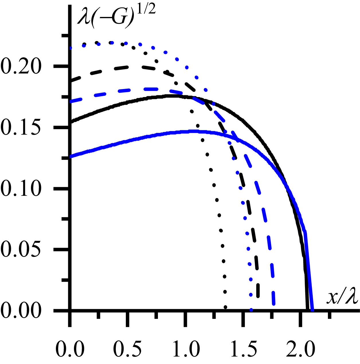
is explained with the help of the curves in figure 10. Two sets of curves are presented there. One set is shown in black, it corresponds to
 $N_{z}=3.0$
. The other set is shown in blue, it relates to higher toroidal refractive index
 $N_{z}=5.0$
. The latter set is presented for comparison in contrast to the first set. Solid curves in figure 10 are calculated for the decay length
 $\lambda =1.5\,{\rm cm}$
, dashed curves correspond to
 $\lambda =2.3\,{\rm cm}$
and dotted curves relate to
 $\lambda =3.1\,{\rm cm}$
. The other plasma parameters are the same as in figure 3.
The optical thickness of the evanescent layer as the area under the curves of
 $\lambda \sqrt{-G}$
as a function of normalised coordinate:
 $N_{z}=3.0$
(black curves),
 $N_{z}=5.0$
(blue curves),
 $\lambda =1.5\,{\rm cm}$
(solid curves),
 $\lambda =2.3\,{\rm cm}$
(dashed curves),
 $\lambda =3.1\,{\rm cm}$
(dotted curves). Here,
 $N_{y}=0.94$
,
 $\varphi =2.687$
,
 $n(0)=10^{18}\,{\rm m}^{-3}$
.

The areas under the curves are equal to the optical thickness of the evanescent layer. Transfer from solid to dashed (and/or from dashed to dotted) curves corresponds to increase of the plasma density decay length. One can see from the comparison of black solid and dashed curves that transfer from a black solid to a black dashed curve is associated with the following change of the areas under the curves. A larger area is lost due to shortening of the evanescent layer than that added due to increase of the evanescent layer depth. The increase of
 $\lambda$
from
 $\lambda =1.5\,{\rm }$
to
 $\lambda =2.3\,{\rm cm}$
causes decrease of optical thickness for the wave with
 $N_{z}=3.0$
and
 $N_{y}=0.94$
from
 $\eta _{0}\approx 0.32$
to
 $\eta _{0}\approx 0.29$
and one observes an increase of the fraction of the transmitted power,
 $T(\eta _{0})$
, in figure 3 from
 $T(\eta _{0})\approx 0.49$
to
 $T(\eta _{0})\approx 0.52$
. Similar decrease of the optical thickness takes place during transfer from the black dashed curve to the black dotted curve.
In contrast to black curves, blue ones demonstrate a larger area under the dashed (dotted) curve than under the solid (dashed) one. A smaller area is lost due to shortening of the evanescent layer than that added due to increase of the evanescent layer depth. The increase of
 $\lambda$
from
 $\lambda =1.5\,{\rm }$
to
 $\lambda =2.3\,{\rm cm}$
causes an increase of the optical thickness for the wave with
 $N_{z}=5.0$
and
 $N_{y}=0.94$
from
 $\eta _{0}\approx 0.28$
to
 $\eta _{0}\approx 0.29$
and a decrease of the fraction of the transmitted power,
 $T(\eta _{0})$
, in figure 3 from
 $T(\eta _{0})\approx 0.53$
to
 $T(\eta _{0})\approx 0.52$
is observed.
Numerical study carried out for larger
 $| N_{y}|$
(specifically, for
 $| N_{y}| =1.88$
) also demonstrates the possibility of
 $T(\eta _{0})$
(3.14) increasing with an increase of
 $\lambda$
. The possibility exhibits itself by intersection of the curves
 $P_{\textit{tran}}/P_{0}$
as the function of
 $\lambda$
related to different
 $N_{z}$
and
 $\varphi$
.
 N⊥2(x)
 N⊥2(x)
 G(x)/k02
 Ny=−0.94
 Ny=0.0
 Ny=+0.94
 Nz=3.0
 φ=2.687
 n(0)=1016m−3
 λ=0.023cm
 Ptran/P0
 λ
 Nz=3.0
 Nz=5.0
 Nz=7.0
 Ny=0.94
 Ny=0
 Ny=−0.94
 φ=2.687
 n(0)=1018m−3
 Ptran/P0
 λ
 φ=1.5
 φ=2.687
 φ=4.5
 Ny=0.94
 Ny=0
 Nz=3.0
 n(0)=1017m−3
 Ptran/P0
 λ
 n(0)=1015m−3
 n(0)=1016m−3
 n(0)=1017m−3
 n(0)=1018m−3
 Ny=0.94
 Ny=0
 Ny=−0.94
 Nz=3.0
 φ=2.687
 Re(Ey)
 x/λ:Ny=+0.94
 Ny=0.0
 Ny=−0.94
 Nz=3.0
 φ=2.687
 n(0)=1015m−3
 λ=1.7cm
 Re(Ey)
 x/λ
 Ny=0.0
 Im(Ey)
 x/λ:Ny=+0.94
 Ny=0.0
 Ny=−0.94
 Nz=3.0
 φ=2.687
 n(0)=1015m−3
 λ=1.7cm
 Nz=5.0
 Nz=5.0
 λ−G
 Nz=3.0
 Nz=5.0
 λ=1.5cm
 λ=2.3cm
 λ=3.1cm
 Ny=0.94
 φ=2.687
 n(0)=1018m−3

 Open access

