1 Introduction
One of the major challenges in the design and development of combustors are thermoacoustic instabilities, which are hard to predict and even more difficult to control. Exemplary applications in the engineering sciences where thermoacoustic instabilities play a major role can be found in Lieuwen & Yang (Reference Lieuwen and Yang2005), among them the complications encountered during the development of the F1 engine for the Apollo mission to the Moon in the 1960s. Currently, thermoacoustic instabilities constitute one of the principal concerns when dealing with lean, premixed combustion, a technological choice taken across many industries to reduce
 $\text{NO}_{x}$
emissions and hence comply with environmental constraints.
Thermoacoustic instabilities arise due to a linear feedback coupling between the unsteady heat release from a heating element and acoustic waves, as proposed by Lord Rayleigh (Reference Rayleigh1945). An example of how this might occur is as follows: perturbations of the flame area generate unsteady heat release which, in turn, acts as a primary source of sound radiation (Dowling & Ffowcs Williams Reference Dowling and Ffowcs Williams1983; Ducruix et al. Reference Ducruix, Schuller, Durox and Candel2003; Candel, Durox & Schuller Reference Candel, Durox and Schuller2004). The generated acoustic waves propagate in the combustor, whose typical shape is susceptible to the development of resonant acoustic modes. Consequently, the acoustic pressure perturbations are partially reflected from the boundary of the geometry and return to the region of unsteady heat release. Upstream velocity fluctuations induced by the acoustic field (Ducruix et al. Reference Ducruix, Schuller, Durox and Candel2003; Poinsot & Veynante Reference Poinsot and Veynante2005), or fuel equivalence ratio perturbations induced by the flow field, cause unsteady heat release at the flame which then closes the feedback loop. In practice, hydrodynamics (Renard et al. Reference Renard, Thévenin, Rolon and Candel2000) and entropy (Marble & Candel Reference Marble and Candel1977; Candel et al. Reference Candel, Durox, Ducruix, Birbaud, Noiray and Schuller2009) mechanisms may also play a role in the feedback mechanism. Based on this description, it follows that interrupting the flame–acoustic coupling would weaken or suppress thermoacoustic instabilities, and indeed this approach is pursued by passive control devices (Putnam Reference Putnam1971; Richards, Straub & Robey Reference Richards, Straub and Robey2003) and by active control strategies (Poinsot et al. Reference Poinsot, Candel, Esposito, Lang and Bourienne1989; McManus, Poinsot & Candel Reference McManus, Poinsot and Candel1993; Annaswamy & Ghoniem Reference Annaswamy and Ghoniem1995; Dowling & Morgans Reference Dowling and Morgans2005; Zhao et al. Reference Zhao, Li, Liu, Zhao, Lu and Wang2018).
Critical for the success of these techniques is the correct capture of the feedback process – still a major challenge for realistic systems (Poinsot Reference Poinsot2017). To add to these difficulties, recent studies have shown that the flame element itself gives rise to a feedback mechanism that does not require acoustic reflections or depend fundamentally on the particular geometry of the combustion chamber. This new type of instability has been labelled intrinsic thermoacoustic instability (Hoeijmakers et al. Reference Hoeijmakers, Kornilov, Lopez Arteaga, de Goey and Nijmeijer2014); its modes are referred to as intrinsic thermoacoustic (ITA) modes (Emmert, Bomberg & Polifke Reference Emmert, Bomberg and Polifke2015).
There is ample theoretical, numerical and experimental evidence (Courtine et al.
Reference Courtine, Selle, Nicoud, Polifke, Silva, Bauerheim and Poinsot2014; Hoeijmakers et al.
Reference Hoeijmakers, Kornilov, Lopez Arteaga, de Goey and Nijmeijer2014; Emmert et al.
Reference Emmert, Bomberg and Polifke2015) that the flame element not only interacts with the acoustic modes of the combustion chamber, but also generates instabilities without acoustic feedback from the boundaries. These ITA modes have been analysed analytically, within low-order network frameworks, where analytic solutions for unstable systems can be obtained even in the presence of no reflection from the boundaries – in contrast to the well-established acoustic feedback loop. The work by Courtine et al. (Reference Courtine, Selle, Nicoud, Polifke, Silva, Bauerheim and Poinsot2014) critically assessed the validity of the theoretical results on ITA modes by applying Crocco’s classical
 $n$
–
 $\unicode[STIX]{x1D70F}$
model and concluded that the model is able to capture the ITA modes. The analytical form of these pure ITA modes is equivalent to outward travelling waves (Hoeijmakers et al.
Reference Hoeijmakers, Kornilov, Lopez Arteaga, de Goey and Nijmeijer2014; Emmert et al.
Reference Emmert, Bomberg and Polifke2015, Reference Emmert, Bomberg, Jaensch and Polifke2017). Their stability is determined by the flame-model parameters only, though Hoeijmakers et al. (Reference Hoeijmakers, Kornilov, Lopez Arteaga, de Goey and Nijmeijer2014) demonstrates that, even for subcritical values of the gain, an appropriate change in the reflection coefficients can still destabilise the system. Experimentally, instabilities have been observed for nearly anechoic conditions at the upstream inlet, with frequencies in good agreement with the theoretical predictions for ITA modes (Hoeijmakers et al.
Reference Hoeijmakers, Kornilov, Lopez Arteaga, de Goey and Nijmeijer2016). In addition, Emmert et al. (Reference Emmert, Meindl, Jaensch and Polifke2016) showed that a stable system can be driven into instability, if excited at intrinsic frequencies. The work by Hosseini et al. (Reference Hosseini, Kornilov, Lopez Arteaga, Polifke, Teerling and de Goey2018) shows that, as the parameters of the system are changed, there is significant interplay between the ITA and the acoustic modes; in particular, they identify a coupling mechanism that causes ITA modes to ‘attach and detach’ from their acoustic counterparts.
Recent work by Mensah et al. (Reference Mensah, Magri, Silva, Buschmann and Moeck2018) and Silva, Yong & Magri (Reference Silva, Yong and Magri2018) identified so-called ‘exceptional points’ of the system, i.e. the parameter combinations for which acoustic and ITA modes coalesce into a degenerate eigenvalue. They show that in the neighbourhood of these points the sensitivities are particularly large. Although not correlated with exceptional points, these regions of large sensitivities in the complex plane were identified previously by Juniper & Sujith (Reference Juniper and Sujith2018). At the exceptional points the eigenvalue sensitivities can no longer be evaluated by a first-order expansion (Mensah et al. Reference Mensah, Magri, Silva, Buschmann and Moeck2018). Further implications for the modelling of the system at such parameter configurations are still open and unresolved.
In light of these rather unexplored instability modes, a comprehensive study is warranted, as it may lead to the development of more accurate design tools for the combustion industry. In particular, the interplay of these ITA modes with the classical thermoacoustic modes needs to be addressed.
Theoretical predictions of thermoacoustic stabilities are generally based on modal (eigenvalue) analysis. Low-order models identify the eigenvalues, which provide frequencies and growth rates of the thermoacoustic modes, and their associated eigenvectors, which describe their spatial shape. The system is deemed stable if all eigenvalues have negative growth rates. This type of analysis, however, provides information about the long-time (Lyapunov) stability of the systems which may differ significantly from the short-time dynamics; in other words, thermoacoustic systems could exhibit transient growth (Schmid & Henningson Reference Schmid and Henningson2001; Schmid Reference Schmid2007). This behaviour is typical of non-normal systems, or systems whose eigenvectors are not orthogonal, and over the past decade thermoacoustic systems have been found both theoretically (Balasubramanian & Sujith Reference Balasubramanian and Sujith2008a
,Reference Balasubramanian and Sujith
b
; Nicoud et al.
Reference Nicoud, Benoit, Sensiau and Poinsot2007; Mariappan & Sujith Reference Mariappan and Sujith2010; Juniper Reference Juniper2011; Mangesius & Polifke Reference Mangesius and Polifke2011; Mariappan, Sujith & Schmid Reference Mariappan, Sujith and Schmid2011; Sujith, Juniper & Schmid Reference Sujith, Juniper and Schmid2016) and experimentally (Wieczorek et al.
Reference Wieczorek, Sensiau, Polifke and Nicoud2011; Zhao Reference Zhao2012; Mariappan, Sujith & Schmid Reference Mariappan, Sujith and Schmid2015) to exhibit non-normal characteristics. These findings are important for the design of combustion systems: firstly, transient growth phenomena may cause significant direct stress to an engine; secondly, they might lead to the triggering of a nonlinear instability (Juniper Reference Juniper2011), once amplification due to transient growth becomes sufficiently large. The non-orthogonality of thermoacoustic modes has been shown analytically and numerically by Nicoud et al. (Reference Nicoud, Benoit, Sensiau and Poinsot2007), and verified in subsequent Galerkin-based studies by Balasubramanian & Sujith (Reference Balasubramanian and Sujith2008a
,Reference Balasubramanian and Sujith
b
) and Magri et al. (Reference Magri, Balasubramanian, Sujith and Juniper2013). Balasubramanian & Sujith (Reference Balasubramanian and Sujith2008b
) investigated the role of transient growth in triggering limit-cycle behaviour and studied how the maximum amplification changed as the heater position and flame time delay varied; growth factors of four to six were reported. Similar amplification was found for variations of the Péclet number and slot half-width (Balasubramanian & Sujith Reference Balasubramanian and Sujith2008a
; Magri et al.
Reference Magri, Balasubramanian, Sujith and Juniper2013). Based on a nonlinear Galerkin model, nonlinear direct-adjoint optimisation was employed by Juniper (Reference Juniper2011) to identify the most likely initial condition that yields triggering of limit-cycle behaviour; the same work attributed triggering to the transient amplification of perturbation energy. The importance of transient effects has further been stressed by Wieczorek et al. (Reference Wieczorek, Sensiau, Polifke and Nicoud2011) who, using the Helmholtz equation, focused attention on the contribution of entropy in the total energy of the flow: augmenting the flow velocity resulted in an increase of non-orthogonality in the modal structures and an increased potential for transient amplification. On the experimental side, Mariappan et al. (Reference Mariappan, Sujith and Schmid2015) demonstrated that modal non-orthogonality increases with growing heater power. The maximum transient energy growth was determined as 2.3, and the associated optimal initial condition corresponded to a linear combination of sine waves of the first and second acoustic modes with similar amplitudes but a
 $90^{\circ }$
phase difference between them. In another study, Zhao (Reference Zhao2012) considered a vertical Rijke tube and investigated the most dangerous flame location as well as the effect on non-orthogonality as mean heat is added. Recently, Blumenthal et al. (Reference Blumenthal, Tangirala, Sujith and Polifke2017) pointed out that non-normal analysis in thermoacoustic systems should be addressed using a carefully selected energy norm. By revisiting previous works, they show that transient growth results can only identify mechanisms linked to the state variables included in the selected norm and have to be interpreted accordingly. As a thermoacoustic system requires the modelling of the feedback from the flame, they follow the semi-norm approach proposed by Foures, Caulfield & Schmid (Reference Foures, Caulfield and Schmid2012) to exclude the unsteady heat release rate from the norm used in an investigation of the maximum energy amplification. Using this technique they analyse a Rijke tube and demonstrate that one of the mechanisms for transient growth relies on a maximisation of a Rayleigh-like term. Furthermore, as the characteristic time scale of the flame response plays a crucial role in transient growth, faster flame responses are found to exhibit larger levels of transient growth.
In summary, previous analyses of the non-normal nature of a Rijke tube conclude that transient growth of acoustic modes is to be expected to contribute to energy amplification by at most a factor of ten; nonlinearities will prevent further growth, as a limit cycle or other nonlinear dynamics (Mariappan & Sujith Reference Mariappan and Sujith2010; Subramanian, Sujith & Wahi Reference Subramanian, Sujith and Wahi2013) is reached and self-sustained oscillations prevail. As these amplification factors are not considered large, recent research efforts have abandoned the study of triggering induced by transient growth.
However, in view of recent findings regarding ITA modes, we perform a non-normal analysis of a Rijke tube, exploring the implications of ITA modes on the sensitivity of the spectrum and the transient amplification of energy. This analysis will employ adjoint techniques together with low-order network models and investigate the pertinent parameter space for the Rijke tube. In § 2 we present the physical set-up for the Rijke tube and state the governing equations. Sections 3 and 4 describe, respectively, the low-order network model and its implementation, and the fully discrete representation. Section 5 provides the mathematical background for the non-modal analysis of our linear system. Modal and non-modal results are shown and discussed in §§ 6 and 7. Concluding remarks are offered in § 8.
2 The Rijke tube: model and governing equations
In this study we investigate the thermoacoustic stability of a simplified combustor taken in the form of a Rijke tube. We start by neglecting the influence of mean flow and mean heat addition. This reduced set-up allows us to more clearly identify and describe the characteristic behaviour of the flame and acoustic modes. The analysis of the problem can be further simplified by treating the flame front as compact, a reasonable assumption when comparing the long acoustic wavelength to the narrow size of the combustion zone (Lieuwen & Yang Reference Lieuwen and Yang2005). Our analysis is concerned only with low frequencies; the associated waves propagate as plane waves in the tube and reduce the problem to one spatial dimension. Furthermore, viscous boundary layer effects are neglected, as the boundary layers are considered far smaller than the tube diameter.
Starting from the one-dimensional Euler equations driven by an unsteady heat-source term, we linearise around a zero mean flow and neglect additions to the mean heat. This results in a uniform temperature in the two sections of the tube, and therefore the same mean flow properties throughout the tube. Under these simplifications, the governing equations for the fluctuating longitudinal velocity
 $u$
and the pressure
 $p$
read
 $$\begin{eqnarray}\displaystyle \left.\begin{array}{@{}c@{}}\displaystyle \frac{\unicode[STIX]{x2202}p}{\unicode[STIX]{x2202}t}+\unicode[STIX]{x1D6FE}\overline{p}\displaystyle \frac{\unicode[STIX]{x2202}u}{\unicode[STIX]{x2202}x}=q(\unicode[STIX]{x1D6FE}-1),\\ \displaystyle \frac{\unicode[STIX]{x2202}u}{\unicode[STIX]{x2202}t}+\displaystyle \frac{\overline{c}^{2}}{\unicode[STIX]{x1D6FE}\overline{p}}\displaystyle \frac{\unicode[STIX]{x2202}p}{\unicode[STIX]{x2202}x}=0,\end{array}\right\} & & \displaystyle\end{eqnarray}$$
bars denoting mean flow properties,
 $q$
representing the unsteady heat release rate per unit area,
 $\unicode[STIX]{x1D6FE}$
being the specific heat ratio and
 $\overline{c}$
denoting the speed of sound. As for boundary conditions, we assume that the Rijke tube is open with loss-free reflections at both ends.
In our following analysis, we will consider two representations of the system: (i) a low-order network model, commonly used to describe such thermoacoustic systems, and (ii) a fully discretised system, facilitating a dynamical-system approach to our problem.
3 The low-order network model
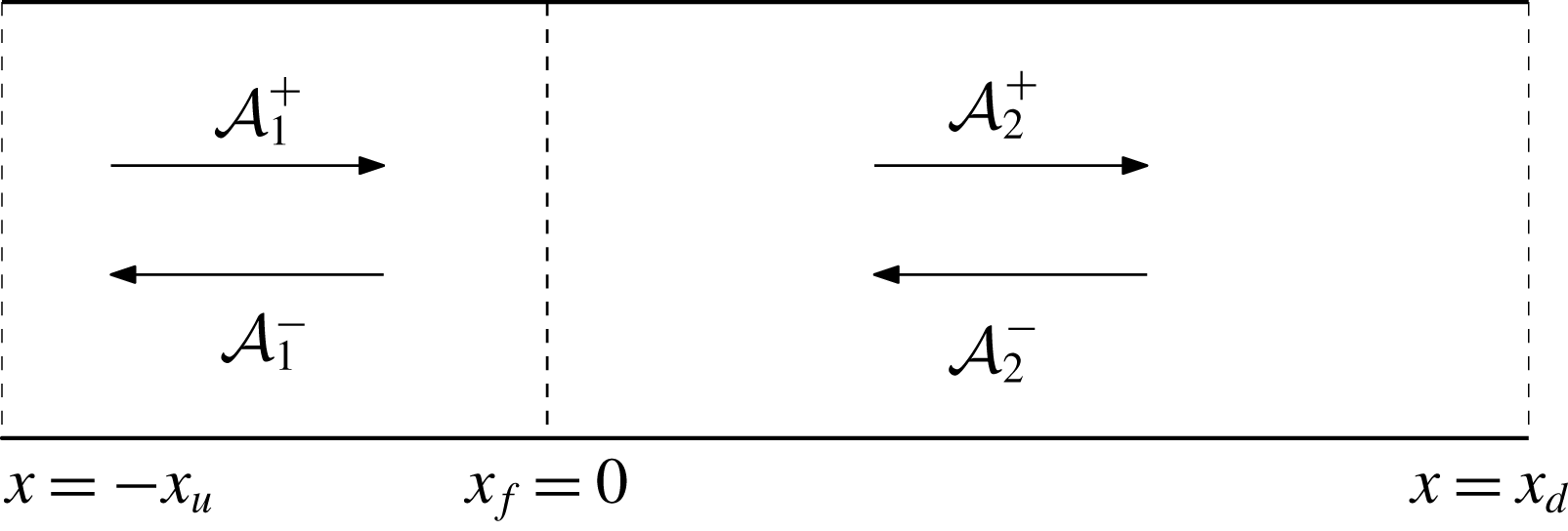
Either side of the flame, equations (2.1) combine to give a one-dimensional wave equation in pressure fluctuation. This means that within the limits of our approximations, we can take advantage of a simplified description of the acoustics in the upstream and downstream sections of the tube and represent the flame by appropriate jump conditions at the flame location (
 $x_{f}$
). The open ends of the Rijke tube (at
 $-x_{u}$
and
 $x_{d}$
) are modelled by appropriate boundary conditions. A schematic of the set-up together with some of the reference parameters is displayed in figure 1. This approximation is generally regarded as a low-order model of a standard Rijke tube, details of which can be found, for example, in McManus et al. (Reference McManus, Poinsot and Candel1993), Dowling & Stow (Reference Dowling and Stow2003) and Sattelmayer & Polifke (Reference Sattelmayer and Polifke2003).
Schematic of the Rijke tube, showing upstream- and downstream-propagating acoustic waves in each section and reference parameters.

The wave forms of the solution of the pressure and velocity perturbations in the upstream and downstream sections of the tube satisfy the wave equation and can be stated as
 $$\begin{eqnarray}\displaystyle & \displaystyle p_{i}={\mathcal{A}}_{i}^{+}\left(t-\frac{x}{\overline{c}}\right)+{\mathcal{A}}_{i}^{-}\left(t+\frac{x}{\overline{c}}\right), & \displaystyle\end{eqnarray}$$
 $$\begin{eqnarray}\displaystyle & \displaystyle u_{i}=\frac{{\mathcal{A}}_{i}^{+}}{\overline{\unicode[STIX]{x1D70C}}\overline{c}}\left(t-\frac{x}{\overline{c}}\right)-\frac{{\mathcal{A}}_{i}^{-}}{\overline{\unicode[STIX]{x1D70C}}\overline{c}}\left(t+\frac{x}{\overline{c}}\right), & \displaystyle\end{eqnarray}$$
where the subscript
 $i=1,2$
corresponds to the respective sections and
 ${\mathcal{A}}_{i}^{\pm }$
represents the travelling wave amplitudes. The model does not include entropy waves, a reasonable approximation for small Mach numbers and open tube ends (Goh & Morgans Reference Goh and Morgans2013).
The flame induces a jump in the acoustic wave strengths across the flame location. The associated conditions follow from applying the quasi-steady linearised conservation laws across the flame (see Dowling Reference Dowling1997; Dowling & Stow Reference Dowling and Stow2003). For our special case (no mean flow and no mean heat release rate), we have
 $$\begin{eqnarray}\displaystyle & \displaystyle p_{2}=p_{1}, & \displaystyle\end{eqnarray}$$
 $$\begin{eqnarray}\displaystyle & \displaystyle u_{2}=u_{1}+\frac{\unicode[STIX]{x1D6FE}-1}{\unicode[STIX]{x1D6FE}\overline{p}}q. & \displaystyle\end{eqnarray}$$
In our simplified set-up, the pressure perturbations are continuous across the flame, while the velocity fluctuations exhibit a discontinuity. To close the system, a flame model, which relates the unsteady heat release rate to the acoustic waves, is needed. We choose the
 $n$
–
 $\unicode[STIX]{x1D70F}$
model (Crocco Reference Crocco1969), properly rescaled for a zero-Mach-number approximation (Morgans & Dowling Reference Morgans and Dowling2007), which relates the unsteady heat release rate
 $q$
(more specifically, its Laplace transform
 $\hat{q}$
) to the velocity perturbations (or its Laplace transform) just upstream of the flame. We have
 $$\begin{eqnarray}\displaystyle {\mathcal{H}}(s)=\frac{1}{\overline{p}\unicode[STIX]{x1D6FE}}\frac{\hat{q}(s)}{\hat{u} _{1}(s)}=n_{f}\text{e}^{-s\unicode[STIX]{x1D70F}_{f}}, & & \displaystyle\end{eqnarray}$$
with
 $s=\unicode[STIX]{x1D70E}+\text{i}\unicode[STIX]{x1D714}$
as the complex eigenfrequency,
 $n_{f}$
denoting the gain and
 $\unicode[STIX]{x1D70F}_{f}$
representing a time lag for the heat release.
The acoustic boundary conditions at the tube ends are prescribed by pressure reflection coefficients
 $R_{u},R_{d}$
linking the outgoing and incoming waves, such that
 ${\mathcal{A}}_{1}^{+}(t)=R_{u}{\mathcal{A}}_{1}^{-}(t-\unicode[STIX]{x1D70F}_{u})$
at the inlet and
 ${\mathcal{A}}_{2}^{-}(t)=R_{d}{\mathcal{A}}_{2}^{+}(t-\unicode[STIX]{x1D70F}_{d})$
at the outlet, with
 $\unicode[STIX]{x1D70F}_{d}=2x_{d}/\overline{c}$
and
 $\unicode[STIX]{x1D70F}_{u}=2x_{u}/\overline{c}$
. For an open–open Rijke tube with loss-free reflections, we take
 $R_{d}=R_{u}=-1$
. The expressions for the wave reflections at the boundaries can also be transformed into the Laplace domain where they read
 $$\begin{eqnarray}\displaystyle {\mathcal{R}}_{u}(s)=\frac{\hat{{\mathcal{A}}}_{1}^{+}}{\hat{{\mathcal{A}}}_{1}^{-}}=R_{u}\text{e}^{-s\unicode[STIX]{x1D70F}_{u}},\quad {\mathcal{R}}_{d}(s)=\frac{\hat{{\mathcal{A}}}_{2}^{-}}{\hat{{\mathcal{A}}}_{2}^{+}}=R_{d}\text{e}^{-s\unicode[STIX]{x1D70F}_{d}}. & & \displaystyle\end{eqnarray}$$
Substituting the wave form of the solutions, also transformed into the Laplace domain, into the flame jump conditions (3.3), (3.4) and boundary conditions (3.6), we can cast our governing system into a matrix form (adapted from Hoeijmakers et al. (Reference Hoeijmakers, Kornilov, Lopez Arteaga, de Goey and Nijmeijer2014)) as follows:
 $$\begin{eqnarray}\displaystyle \underbrace{\left[\begin{array}{@{}cccc@{}}{\mathcal{T}}_{a}(s) & {\mathcal{T}}_{b}(s) & -1 & 0\\ {\mathcal{T}}_{b}(s) & {\mathcal{T}}_{a}(s) & 0 & -1\\ 1 & -{\mathcal{R}}_{u}(s) & 0 & 0\\ 0 & 0 & -{\mathcal{R}}_{d}(s) & 1\\ \end{array}\right]}_{\unicode[STIX]{x1D648}}\left[\begin{array}{@{}c@{}}\hat{{\mathcal{A}}}_{1}^{+}\\ \hat{{\mathcal{A}}}_{1}^{-}\\ \hat{{\mathcal{A}}}_{2}^{+}\\ \hat{{\mathcal{A}}}_{2}^{-}\\ \end{array}\right]=0, & & \displaystyle\end{eqnarray}$$
with
 ${\mathcal{T}}_{a}(s)=(1/2\sqrt{T_{r}})(1+\unicode[STIX]{x1D703}{\mathcal{H}}(s)+\sqrt{T_{r}})$
and
 ${\mathcal{T}}_{b}(s)=(1/2\sqrt{T_{r}})(-1-\unicode[STIX]{x1D703}{\mathcal{H}}(s)+\sqrt{T_{r}})$
, where
 $\unicode[STIX]{x1D703}=\unicode[STIX]{x1D6FE}-1$
and
 $T_{r}$
denotes the temperature ratio across the flame, which in our case is
 $T_{r}=1$
, as we neglect mean heat addition. Requiring non-trivial solutions of the above system results in a dispersion relation for the complex eigenfrequency
 $s=\unicode[STIX]{x1D70E}+\text{i}\unicode[STIX]{x1D714}$
. Mathematically, we require a zero determinant of the matrix
 $\unicode[STIX]{x1D648}$
. We obtain
 $$\begin{eqnarray}\det (\unicode[STIX]{x1D648})={\mathcal{T}}_{a}-{\mathcal{R}}_{d}{\mathcal{T}}_{b}+{\mathcal{R}}_{u}{\mathcal{T}}_{b}-{\mathcal{R}}_{d}{\mathcal{R}}_{u}{\mathcal{T}}_{a}=0.\end{eqnarray}$$
While this dispersion relation (a nonlinear eigenvalue problem) has to be solved numerically in all generality, for special cases, analytical forms for the acoustic and ITA modes can be extracted.
For the case of no unsteady heat addition (i.e. no flame in the tube), the determinant reduces to
 $R_{u}R_{d}\text{e}^{-s(\unicode[STIX]{x1D70F}_{u}+\unicode[STIX]{x1D70F}_{d})}-1=0$
and the dispersion relation for the classical acoustic modes is recovered (Hoeijmakers et al.
Reference Hoeijmakers, Kornilov, Lopez Arteaga, de Goey and Nijmeijer2014):
 $$\begin{eqnarray}\displaystyle \left\{\begin{array}{@{}c@{}}\unicode[STIX]{x1D714}=\displaystyle \frac{2j\unicode[STIX]{x03C0}}{\unicode[STIX]{x1D70F}_{l}},\\ \unicode[STIX]{x1D70E}=-\displaystyle \frac{1}{\unicode[STIX]{x1D70F}_{l}}\ln \left(\displaystyle \frac{1}{R_{u}R_{d}(-1)^{2j}}\right),\end{array}\quad \text{with }j\in \mathbb{Z},\right. & & \displaystyle\end{eqnarray}$$
where
 $\unicode[STIX]{x1D70F}_{l}=\unicode[STIX]{x1D70F}_{u}+\unicode[STIX]{x1D70F}_{d}$
.
For the case of no acoustic modes, we set the tube end reflection coefficients to zero. This case represents an anechoic situation, eliminates the organ pipe modes and highlights the presence of ITA modes. The form of the determinant is simply
 $\unicode[STIX]{x1D703}{\mathcal{H}}(s)+2=0$
, which results in the following dispersion relation (Hoeijmakers et al.
Reference Hoeijmakers, Kornilov, Lopez Arteaga, de Goey and Nijmeijer2014):
 $$\begin{eqnarray}\displaystyle \left\{\begin{array}{@{}c@{}}\unicode[STIX]{x1D714}=\displaystyle \frac{\unicode[STIX]{x03C0}(2k-1)}{\unicode[STIX]{x1D70F}_{f}},\\ \unicode[STIX]{x1D70E}=-\displaystyle \frac{1}{\unicode[STIX]{x1D70F}_{f}}\ln \left(\displaystyle \frac{-2}{(-1)^{2k-1}\unicode[STIX]{x1D703}n_{f}}\right),\end{array}\quad \text{with }k\in \mathbb{Z}.\right. & & \displaystyle\end{eqnarray}$$
A third special case results for identical upstream and downstream reflection coefficients (
 ${\mathcal{R}}_{d}={\mathcal{R}}_{u}$
). This configuration can be achieved by placing the flame at the centre of the tube (for open–open and closed–closed tube arrangements; the flame is then at a velocity node for half of the acoustic modes). In this case, both acoustic and ITA modes satisfy, respectively, (3.9) and (3.10) without taking either the reflection coefficients or the flame gain as zero. The dispersion relation can mathematically be factored as
 $$\begin{eqnarray}\displaystyle \det (\unicode[STIX]{x1D648}) & = & \displaystyle {\mathcal{T}}_{a}-{\mathcal{R}}_{d}{\mathcal{R}}_{u}{\mathcal{T}}_{a}=0\nonumber\\ \displaystyle & = & \displaystyle {\mathcal{T}}_{a}(1-{\mathcal{R}}_{d}{\mathcal{R}}_{u})=0.\end{eqnarray}$$
Hence, the different modes can be identified separately.
Besides the dispersion relation, which identifies and tracks the various eigenvalues in the complex plane as the governing parameters are varied, we are also interested in the sensitivity of the eigenvalues to changes in the system parameters. Sensitivity results have been used recently in optimisation studies of thermoacoustic low-order network models that target specifically the growth rates of the eigenvalues (Aguilar & Juniper Reference Aguilar and Juniper2018; Yang et al.
Reference Yang, Sogaro, Morgans and Schmid2019). While aimed towards the design of thermoacoustically stable systems, such optimisations do not provide specific insight into the interplay of different types of modes. Derivations of adjoint-based sensitivities for the network model set-up can be found in Magri & Juniper (Reference Magri and Juniper2014), Magri, Bauerheim & Juniper (Reference Magri, Bauerheim and Juniper2016) and Aguilar, Magri & Juniper (Reference Aguilar, Magri and Juniper2017); we therefore omit the derivation and state the expression for the sensitivity of the system’s non-degenerate
 $i$
th eigenvalue,
 $s_{i}$
, to perturbations in the
 $j$
th parameter, denoted by
 $g_{j}$
, as
 $$\begin{eqnarray}\frac{\unicode[STIX]{x2202}s_{i}}{\unicode[STIX]{x2202}g_{j}}=-\frac{(\boldsymbol{a}_{i}^{\dagger })^{H}\displaystyle \frac{\unicode[STIX]{x2202}\unicode[STIX]{x1D648}}{\unicode[STIX]{x2202}g_{j}}\boldsymbol{a}_{i}}{(\boldsymbol{a}_{i}^{\dagger })^{H}\displaystyle \frac{\unicode[STIX]{x2202}\unicode[STIX]{x1D648}}{\unicode[STIX]{x2202}s_{i}}\boldsymbol{a}_{i}},\end{eqnarray}$$
where the superscript ‘
 $H$
’ stands for the complex conjugate transpose,
 $\boldsymbol{a}_{i}$
denotes the direct eigenvector corresponding to the
 $i^{\text{i}t}$
eigenvalue and
 $\boldsymbol{a}_{i}^{\dagger }$
represents the adjoint eigenvector obtained by the solution of the adjoint problem
 $(\boldsymbol{a}_{i}^{\dagger })^{H}\unicode[STIX]{x1D648}=0$
.
4 The fully discretised time-domain model
Non-modal analysis provides a tool for analysing the interplay of the modes. To proceed along this line, we require a representation of the system as a temporal evolution problem. We choose the model used by Sayadi et al. (Reference Sayadi, LeChenadec, Schmid, Richecoeur and Massot2014) which accurately captures the velocity jump condition across the flame. The governing equations are identical to (2.1), and the flame model is implemented directly as the inverse Laplace transform of expression (3.5). We have also included acoustic damping (denoted by
 $\unicode[STIX]{x1D701}$
) as in Balasubramanian & Sujith (Reference Balasubramanian and Sujith2008a
), Juniper (Reference Juniper2011) and Sayadi et al. (Reference Sayadi, LeChenadec, Schmid, Richecoeur and Massot2014) to empirically account for acoustic losses in the system. The governing equations read
 $$\begin{eqnarray}\displaystyle \left.\begin{array}{@{}c@{}}\displaystyle \frac{\unicode[STIX]{x2202}p}{\unicode[STIX]{x2202}t}=-\unicode[STIX]{x1D6FE}\overline{p}\displaystyle \frac{\unicode[STIX]{x2202}u}{\unicode[STIX]{x2202}x}-\displaystyle \frac{\overline{c}}{L}\unicode[STIX]{x1D701}\ast p+(\unicode[STIX]{x1D6FE}-1)\unicode[STIX]{x1D6FE}\overline{p}n_{f}\unicode[STIX]{x1D6FF}_{x_{f}}u(t-\unicode[STIX]{x1D70F}_{f}),\\ \displaystyle \frac{\unicode[STIX]{x2202}u}{\unicode[STIX]{x2202}t}=-\displaystyle \frac{\overline{c}^{2}}{\unicode[STIX]{x1D6FE}\overline{p}}\displaystyle \frac{\unicode[STIX]{x2202}p}{\unicode[STIX]{x2202}x},\end{array}\right\} & & \displaystyle\end{eqnarray}$$
where
 $\unicode[STIX]{x1D6FF}_{x_{f}}$
is the Dirac function centred at
 $x_{f}$
and
 $\ast$
represents the convolution operator. The model for the acoustic damping follows Sterling & Zukoski (Reference Sterling and Zukoski1991) and Matveev & Culick (Reference Matveev and Culick2003) with
 $\unicode[STIX]{x1D701}_{j}=b_{1}j^{2}+b_{2}\sqrt{j}$
. In the present study, instead of using typical values for
 $b_{1}$
and
 $b_{2}$
as found in Juniper (Reference Juniper2011) and Subramanian et al. (Reference Subramanian, Sujith and Wahi2013), we set the parameters to
 $1\times 10^{-5}$
in order to match the set-up of the low-order network system. Equation (4.1) represents a delayed partial differential equation. It is discretised in space using a staggered grid with
 $N=155$
collocation points and compact finite differences (Lele Reference Lele1992; Nagarajan, Lele & Ferziger Reference Nagarajan, Lele and Ferziger2003) to represent spatial derivatives (see Sayadi et al. (Reference Sayadi, LeChenadec, Schmid, Richecoeur and Massot2014) for details). The semi-discretised equation constitutes a system of ordinary delay-differential equations. Introducing
 $\boldsymbol{p}$
and
 $\boldsymbol{u}$
as the pressure and velocity vectors on the staggered grid, we define the state variable
 $\boldsymbol{x}=[\boldsymbol{p},\boldsymbol{u}]^{\text{T}}$
and obtain the system
 $$\begin{eqnarray}\dot{\boldsymbol{x}}=\unicode[STIX]{x1D63C}_{0}\boldsymbol{x}(t)+\unicode[STIX]{x1D63C}_{1}\boldsymbol{x}(t-\unicode[STIX]{x1D70F}_{f}),\end{eqnarray}$$
where the matrix
 $\unicode[STIX]{x1D63C}_{0}$
contains all spatial derivatives and damping, while the matrix
 $\unicode[STIX]{x1D63C}_{1}$
accounts for the (discontinuous) flame effects discretised with a ghost fluid method (Fedkiw et al.
Reference Fedkiw, Aslam, Merriman and Osher1999).
For the above time-delay system, the associated characteristic equation (dispersion relation) reads
 $$\begin{eqnarray}(-\unicode[STIX]{x1D706}\unicode[STIX]{x1D644}+\unicode[STIX]{x1D63C}_{0}+\unicode[STIX]{x1D63C}_{1}\text{e}^{-\unicode[STIX]{x1D70F}_{f}\unicode[STIX]{x1D706}})\boldsymbol{x}=0.\end{eqnarray}$$
The above equation is in the form of a nonlinear eigenvalue problem due to the appearance of the eigenvalue
 $\unicode[STIX]{x1D706}$
in the exponential term. In what follows, we use the infinitesimal generator discretisation (IGD) method, as proposed in Jarlebring (Reference Jarlebring2008), to solve the delay-differential equation.
The method transforms the ordinary delay-differential equation into a partial differential equation by introducing a ‘memory’ coordinate
 $\unicode[STIX]{x1D703}$
. The memory domain spans the time interval
 $\unicode[STIX]{x1D703}\in [t-\unicode[STIX]{x1D70F},t]$
. Along this dimension, information simply advects from time
 $t-\unicode[STIX]{x1D70F}$
to the current state at
 $t$
. A proof of equivalence between the delay-differential equation and the embedded partial differential equation is provided in Jarlebring (Reference Jarlebring2008). Under the IGD scheme, the delay-differential equation
 $$\begin{eqnarray}\displaystyle \left.\begin{array}{@{}c@{}}\displaystyle {\dot{x}}=\unicode[STIX]{x1D63C}_{0}\boldsymbol{x}(t)+\unicode[STIX]{x1D63C}_{1}\boldsymbol{x}(t-\unicode[STIX]{x1D70F}_{f}),\quad t\geqslant 0,\\ \displaystyle \boldsymbol{x}=\boldsymbol{x}_{0}(t),\quad t\in [-\unicode[STIX]{x1D70F}_{f},0],\end{array}\right\} & & \displaystyle\end{eqnarray}$$
transforms into
 $$\begin{eqnarray}\displaystyle \left.\begin{array}{@{}c@{}}\displaystyle \frac{\unicode[STIX]{x2202}\boldsymbol{v}}{\unicode[STIX]{x2202}t}=\displaystyle \frac{\unicode[STIX]{x2202}\boldsymbol{v}}{\unicode[STIX]{x2202}\unicode[STIX]{x1D703}},\quad t\geqslant 0,\unicode[STIX]{x1D703}\in [-\unicode[STIX]{x1D70F}_{f},0],\\ \displaystyle \left.\frac{\unicode[STIX]{x2202}\boldsymbol{v}}{\unicode[STIX]{x2202}\unicode[STIX]{x1D703}}\right|_{(t,0)}=\unicode[STIX]{x1D63C}_{1}\boldsymbol{v}(t,-\unicode[STIX]{x1D70F}_{f})+\unicode[STIX]{x1D63C}_{0}\boldsymbol{v}(t,0),\quad t\geqslant 0,\\ \displaystyle \boldsymbol{v}(0,\unicode[STIX]{x1D703})=\boldsymbol{x}_{0}(\unicode[STIX]{x1D703}),\end{array}\right\} & & \displaystyle\end{eqnarray}$$
where
 $\boldsymbol{v}(t,\unicode[STIX]{x1D703})$
is equivalent to
 $\boldsymbol{x}(t-\unicode[STIX]{x1D703})$
. We discretise the memory coordinate
 $\unicode[STIX]{x1D703}$
using 30 Chebyshev polynomials, collocated on Gauss–Lobatto points (Jarlebring Reference Jarlebring2008), and write the full problem as a discrete system of linear ordinary differential equations:
 $$\begin{eqnarray}\frac{\unicode[STIX]{x2202}\boldsymbol{v}}{\unicode[STIX]{x2202}t}=\frac{\unicode[STIX]{x2202}\boldsymbol{v}}{\unicode[STIX]{x2202}\unicode[STIX]{x1D703}}\rightarrow \frac{\unicode[STIX]{x2202}\boldsymbol{v}}{\unicode[STIX]{x2202}t}=\unicode[STIX]{x1D63C}\boldsymbol{v}.\end{eqnarray}$$
It is worth noting that the IGD technique results in a higher-dimensional problem owing to the additional memory coordinate to the one-dimensional spatial discretisation. In particular, the eigenvectors of the full operator represent mode shapes of a two-dimensional problem as they include memory information. In previous investigations, this memory dimension has been treated by ‘freezing’ the associated degrees of freedom and by setting them to zero (Juniper Reference Juniper2011), therefore disregarding the response of the system due to memory effects. We will show that transient growth relies notably on excitations in the memory dimension, which translates into a dependency on past time signals.
The calculation of energy growth and of pseudospectra requires the definition of a matrix norm for
 $\unicode[STIX]{x1D63C}$
. The physical weighting of the state vector components and the weights stemming from the discretisation (in the spatial and memory direction) can be combined into a positive definite weight matrix which, in turn, can be decomposed into its Cholesky factors
 $\unicode[STIX]{x1D652}$
. The acoustic energy integral can then be written as
 $$\begin{eqnarray}\displaystyle \frac{1}{2}\int _{\unicode[STIX]{x1D703}}\int _{L}\left(\displaystyle \frac{1}{\unicode[STIX]{x1D6FE}\overline{p}}p^{2}+\overline{\unicode[STIX]{x1D70C}}u^{2}\right)\text{d}x\,\text{d}\unicode[STIX]{x1D703}=\boldsymbol{v}^{H}\unicode[STIX]{x1D652}^{H}\unicode[STIX]{x1D652}\boldsymbol{v}=\langle \unicode[STIX]{x1D652}\boldsymbol{v},\unicode[STIX]{x1D652}\boldsymbol{v}\rangle =\Vert \unicode[STIX]{x1D652}\boldsymbol{v}\Vert _{2}^{2}. & & \displaystyle\end{eqnarray}$$
As the memory dimension is discretised on Gauss–Lobatto points, we use Clenshaw–Curtis quadrature weights for representing the integral in this coordinate direction (Trefethen & Embree Reference Trefethen and Embree2005).
Before proceeding, we wish to justify our choice of norm in light of the work of Blumenthal et al. (Reference Blumenthal, Tangirala, Sujith and Polifke2017). The above integral is taken over both the spatial and the memory direction. We stress that this choice implies that the acoustic energy is integrated over a period of time equivalent to
 $\unicode[STIX]{x1D70F}_{f}$
, and therefore not instantaneous. This, however, does not include non-acoustic state variables (which can arise from separately modelling the flame’s unsteady heat release), and thus transient growth investigations will not show any short-term amplification resulting from non-acoustic sources.
5 Non-modal analysis
Non-normal linear systems can exhibit short-time characteristics that are significantly different from the long-time dynamics described by the eigenvalues. Transient energy amplification or the pseudoresonance are such non-modal phenomena. For a linear initial-value problem of the form
 $$\begin{eqnarray}\frac{\text{d}\boldsymbol{v}}{\text{d}t}=\unicode[STIX]{x1D63C}\boldsymbol{v},\end{eqnarray}$$
the formal solution can be stated in terms of the matrix exponential
 $$\begin{eqnarray}\boldsymbol{v}(t)=\text{e}^{t\unicode[STIX]{x1D63C}}\boldsymbol{v}(0),\end{eqnarray}$$
which constitutes a mapping of the initial condition
 $\boldsymbol{v}(0)$
onto a solution of (5.1) at a later time
 $t$
. As we are interested in the energy evolution of the system, we will concentrate on
 $$\begin{eqnarray}G(t)=\max _{\Vert \boldsymbol{v}(0)\Vert =1}\sqrt{\langle \boldsymbol{v}(t),\boldsymbol{ v}(t)\rangle }=\max _{\Vert \boldsymbol{v}(0)\Vert =1}\Vert \boldsymbol{v}(t)\Vert =\max _{\Vert \boldsymbol{v}(0)\Vert =1}\Vert \text{e}^{t\unicode[STIX]{x1D63C}}\boldsymbol{v}(0)\Vert =\Vert \text{e}^{t\unicode[STIX]{x1D63C}}\Vert .\end{eqnarray}$$
The maximum energy amplification of any unit-norm initial condition will be governed by
 $\Vert \text{e}^{t\unicode[STIX]{x1D63C}}\Vert$
. The particular choice of norm to measure the size of the evolution operator above can be accounted for by replacing the matrix
 $\unicode[STIX]{x1D63C}$
by a similarity-transformed matrix
 $\unicode[STIX]{x1D63D}$
according to
 $$\begin{eqnarray}\unicode[STIX]{x1D63D}=\unicode[STIX]{x1D652}\unicode[STIX]{x1D63C}\unicode[STIX]{x1D652}^{-1},\end{eqnarray}$$
using the weight matrix
 $\unicode[STIX]{x1D652}$
introduced above. We are also interested in identifying the initial condition
 $\boldsymbol{v}(0)$
that achieves the maximum (transient) energy growth at a specific time
 $t^{\star }$
: a singular value decomposition of
 $\text{e}^{t^{\star }\unicode[STIX]{x1D63D}}$
will furnish this optimal initial condition (Schmid & Henningson Reference Schmid and Henningson2001).
In general, the evolution of
 $\Vert \text{e}^{t\unicode[STIX]{x1D63D}}\Vert$
can be quantified or approximated at three different times of interest (Trefethen & Embree Reference Trefethen and Embree2005): at asymptotically large times (
 $t\rightarrow \infty$
), at intermediate times and at very short times (
 $t=0^{+}$
). The proper quantities to investigate these different regimes can be found in Schmid & Henningson (Reference Schmid and Henningson2001) and, specifically for thermoacoustic systems, in Sujith et al. (Reference Sujith, Juniper and Schmid2016). We briefly state the final results.
5.1 Asymptotic large-time behaviour (
 $t\rightarrow \infty$
)

In the asymptotic limit of large times, the matrix exponential norm is governed by the least stable eigenvalue of
 $\unicode[STIX]{x1D63D}$
. In this case, the spectrum of
 $\unicode[STIX]{x1D63D}$
, denoted by
 $\unicode[STIX]{x1D6EC}(\unicode[STIX]{x1D63D})$
, accurately describes the long-term behaviour.
5.2 Transient behaviour at intermediate times
In this case, the matrix exponential norm gives an accurate account of the linear dynamics. Approximations of the maximum transient energy growth
 $G_{max}=\max _{t\geqslant 0}G(t)$
can be derived (Trefethen & Embree Reference Trefethen and Embree2005), resulting in the definition of the Kreiss constant
 $K$
:
 $$\begin{eqnarray}K(\unicode[STIX]{x1D63D})=\sup _{\text{Re}\,z>0}\text{Re}(z)\Vert (z\unicode[STIX]{x1D644}-\unicode[STIX]{x1D63D})^{-1}\Vert ,\end{eqnarray}$$
with
 $z\in \mathbb{C}$
and
 $\unicode[STIX]{x1D644}$
as the identity matrix. The Kreiss constant
 $K$
represents the ratio of the value of a particular resolvent contour (see the definition of the pseudospectrum below) and its protrusion into the unstable part of the complex plane. It can be shown (Trefethen & Embree Reference Trefethen and Embree2005) that the Kreiss constant provides a lower bound on the maximum transient energy growth
 $G_{max}$
.
5.3 Short-time behaviour (
$t=0^{+}$
)

The short-time dynamics of non-normal linear systems indicates the potential for transient growth. It provides a measure of ‘how fast’ energy can be amplified. The quantity to compute and investigate is the numerical abscissa (Trefethen & Embree Reference Trefethen and Embree2005) of
 $\unicode[STIX]{x1D63D}$
or, expressed equivalently, the maximum protrusion of the numerical range into the unstable half-plane (see Horn & Johnson Reference Horn and Johnson1991). The value of this protrusion is directly linked to the slope of
 $G(t)$
at
 $t=0^{+}$
.
The above quantities will be analysed for our thermoacoustic system, in particular as they relate to the acoustic and ITA structures. They are closely related to the
 $\unicode[STIX]{x1D716}$
-pseudospectra
 $\unicode[STIX]{x1D6EC}_{\unicode[STIX]{x1D716}}$
of the operator
 $\unicode[STIX]{x1D63D}$
(Trefethen & Embree Reference Trefethen and Embree2005) defined as
 $$\begin{eqnarray}\unicode[STIX]{x1D6EC}_{\unicode[STIX]{x1D716}}(\unicode[STIX]{x1D63D})=\{z\in \mathbb{C}:\Vert (z\unicode[STIX]{x1D644}-\unicode[STIX]{x1D63D})^{-1}\Vert \geqslant \unicode[STIX]{x1D716}^{-1}\}.\end{eqnarray}$$
In words, the
 $\unicode[STIX]{x1D716}$
-pseudospectrum of the matrix
 $\unicode[STIX]{x1D63D}$
is the part of the complex plane where the resolvent norm of the operator is greater than a positive
 $\unicode[STIX]{x1D716}^{-1}$
. This definition is equivalent to (Reddy, Schmid & Henningson Reference Reddy, Schmid and Henningson1993; Trefethen Reference Trefethen1999)
 $$\begin{eqnarray}\unicode[STIX]{x1D6EC}_{\unicode[STIX]{x1D716}}(\unicode[STIX]{x1D63D})=\{z\in \mathbb{C}:\unicode[STIX]{x1D6EC}(\unicode[STIX]{x1D63D}+\unicode[STIX]{x1D640})\text{ for a perturbation matrix }\unicode[STIX]{x1D640}\in \mathbb{C}^{N\times N}\text{ with }\Vert \unicode[STIX]{x1D640}\Vert \leqslant \unicode[STIX]{x1D716}\},\end{eqnarray}$$
where
 $N$
is the dimension of the vector space. The above establishes a relationship between the sensitivity of eigenvalues to perturbations in
 $\unicode[STIX]{x1D63D}$
of order
 $\unicode[STIX]{x1D716}$
and the resolvent norm contours. This link will be further explored below, together with the sensitivity of individual eigenvalues to structured, parametric perturbations.
In what follows, the
 $\unicode[STIX]{x1D716}$
-pseudospectra are computed using a shift-invert Arnoldi method as described in Toh & Trefethen (Reference Toh and Trefethen1996) and Wright & Trefethen (Reference Wright and Trefethen2001).
The maximum energy amplification analysis together with the investigation of the most dangerous initial condition, as explained, has been performed using the full norm given by (4.7). Alternatively, it can also be based on the instantaneous acoustic energy. This can be done by using either the methodology proposed by Blumenthal et al. (Reference Blumenthal, Tangirala, Sujith and Polifke2017) or the technique used by Skene & Schmid (Reference Skene and Schmid2019). For completeness, we have also investigated transient growth by maximising the instantaneous acoustic energy, using the methodology from Skene & Schmid (Reference Skene and Schmid2019). The results, while not shown here, are qualitatively similar and match the results performed with the full norm.
6 Results: low-order network model
We commence by analysing the low-order network model, probing its spectral properties, the interplay of acoustic and ITA modes and their sensitivities to parameter changes. Before proceeding, we explicitly state how we classify acoustic and ITA modes. We distinguish if a mode is behaving in an acoustic or intrinsic manner based on the proximity of the eigenvalue to the trajectories of either the pure acoustic or pure ITA modes defined by (3.9) and (3.10), respectively. Each trajectory is obtained by evaluating (3.9) or (3.10), respectively, for each incremental change of the time delay in the chosen range. Practically, we have implemented this using only the growth rates, as the ITA modes in our cases are strongly damped. This definition is different from the one proposed in previous work (Hoeijmakers et al. Reference Hoeijmakers, Kornilov, Lopez Arteaga, de Goey and Nijmeijer2014; Emmert et al. Reference Emmert, Bomberg and Polifke2015; Hosseini et al. Reference Hosseini, Kornilov, Lopez Arteaga, Polifke, Teerling and de Goey2018), where a mode is classified as ITA (or acoustic) based on the limit of reducing the flame gain (reflection coefficients) to zero. Our choice is based on the argument that, as the parameters of the system are changed, the behaviour of the modes can alternate between the two types (see discussion of figure 3). Therefore, classifying a mode by taking a limit, which implies changing a parameter, is for our work less relevant, in view of the aim of understanding the sensitivities of the modes in the current system configuration.
Parameter settings for the open-ended Rijke tube configuration.

6.1 Interplay between acoustic and ITA modes
The parameters of the open-ended Rijke tube configuration are shown in table 1. The following acoustic time scale
 $t^{\ast }=L/\overline{c}$
is used for normalisation. We begin with an overview of the behaviour of the modes as we change
 $\unicode[STIX]{x1D70F}_{f}$
for two locations of the flame: a slightly perturbed case from the symmetric configuration with
 $x_{f}=0.48L$
(figure 2; supplementary movie 1 available at https://doi.org/10.1017/jfm.2019.632) and a more pronounced one with
 $x_{f}=0.4L$
(figure 3; supplementary movie 2).
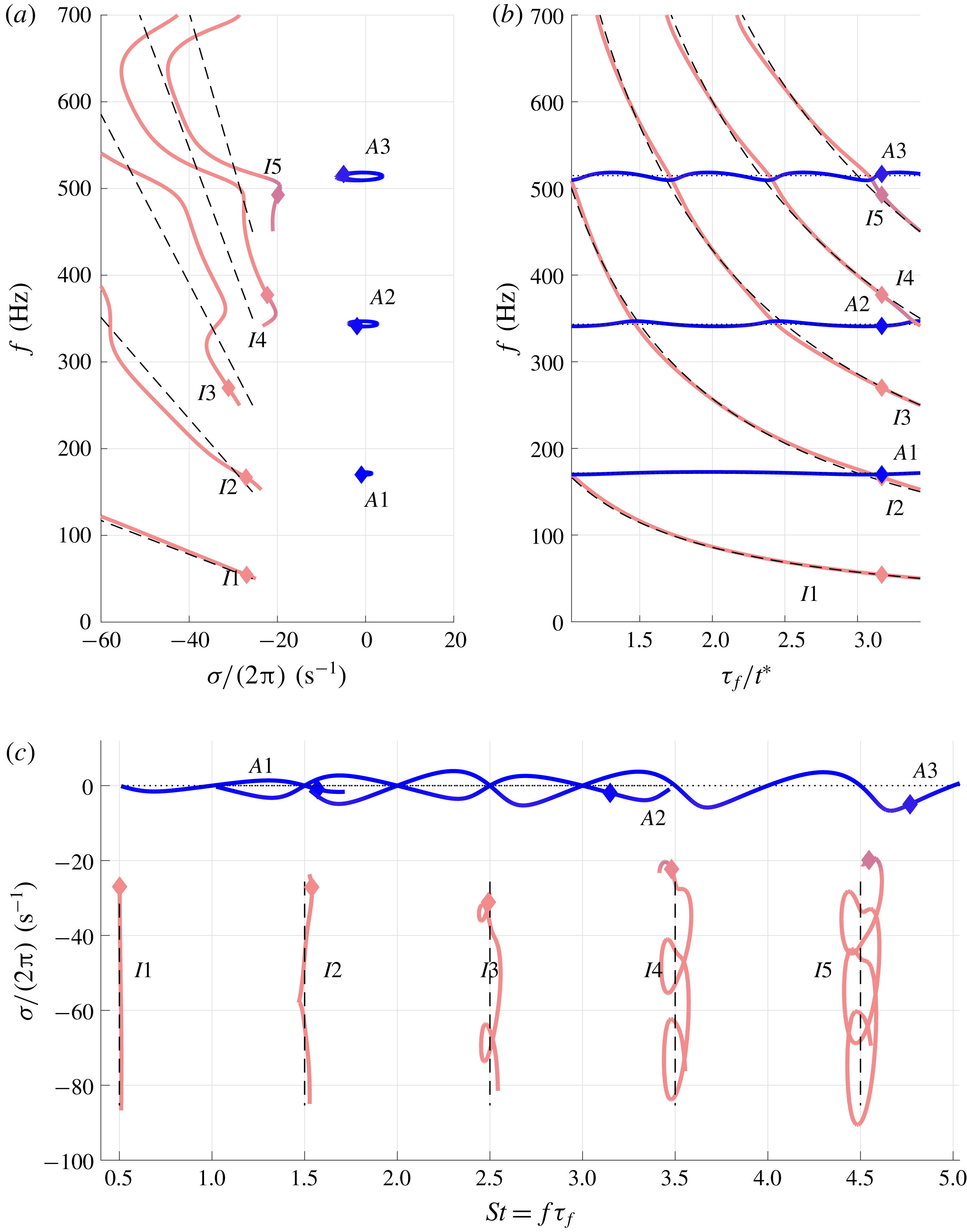
Case
 $x_{f}=0.48L$
. Loci of the acoustic (blue) and ITA (pink) modes in the complex plane (a), frequency behaviour as the flame time delay is changed (b) and growth rate against Strouhal number (c). The loci have been colour coded based on their location in the complex plane. Locations near the imaginary axis (
 $\unicode[STIX]{x1D70E}/(2\unicode[STIX]{x03C0})>-10~\text{s}^{-1}$
) are in dark blue (dark grey in the black-and-white version) and for
 $\unicode[STIX]{x1D70E}/(2\unicode[STIX]{x03C0})<-20~\text{s}^{-1}$
we use light pink (light grey). The range in between changes colour linearly. Superimposed are the analytical values of the pure ITA (dashed lines, (3.10)) and pure acoustic (dotted lines, (3.9)) modes, which also correspond to the solutions of the symmetric case
 $(x_{f}=0.5L)$
. In (a) the movement of the acoustic modes, as the flame time delay is increased, is clockwise, while the ITA modes move towards the lower-right corner of the panel. The diamond (♦) marks an example location of the modes when
 $\unicode[STIX]{x1D70F}_{f}/t^{\ast }=3.16$
. The modes are labelled as either
 $I$
, ITA; or
 $A$
, acoustic. The figure is also available as an animation as supplementary movie 1.

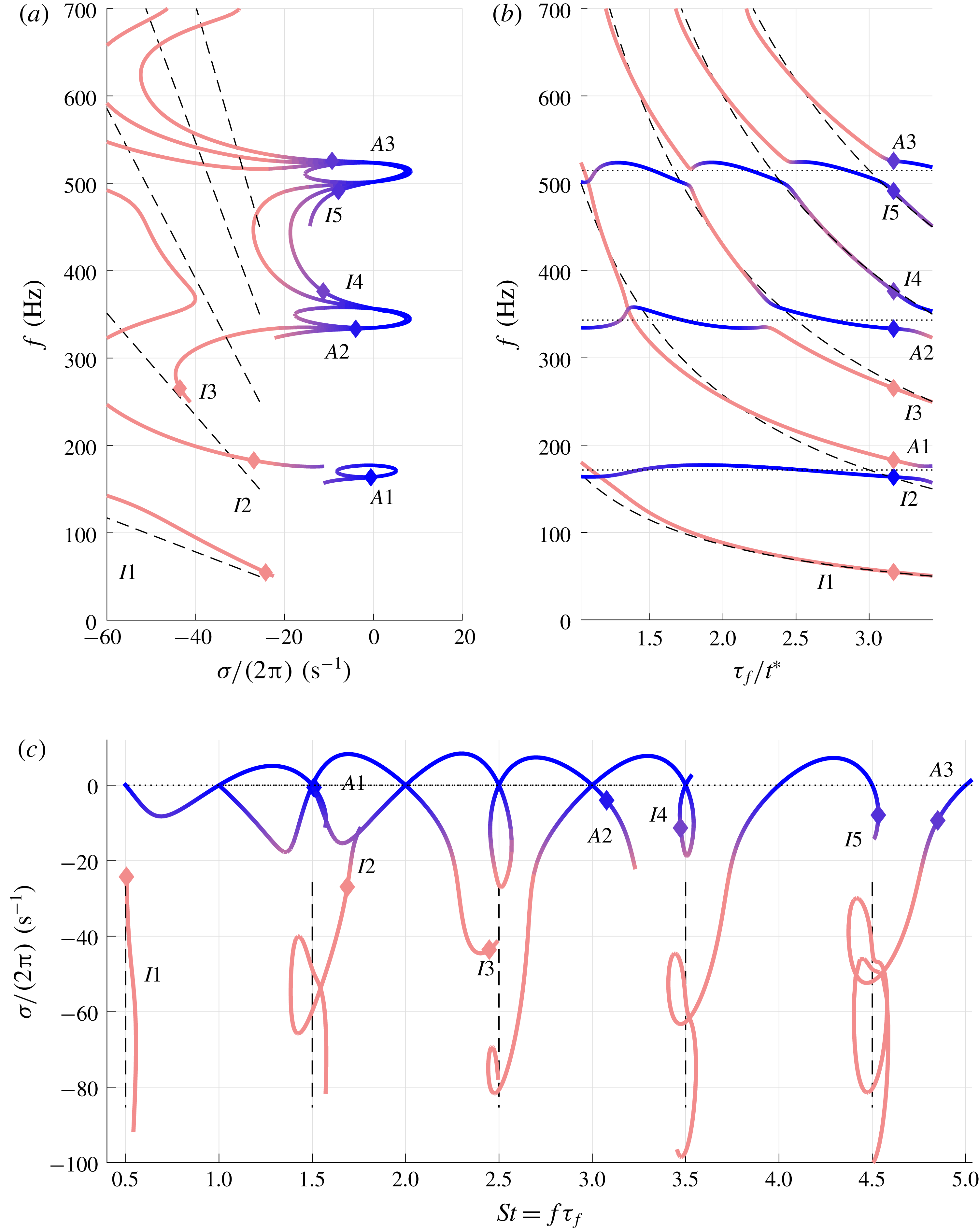
Case
 $x_{f}=0.40L$
. Loci of the acoustic and ITA modes in the complex plane (a), frequency behaviour as the flame time delay is changed (b) and growth rate against Strouhal number (c). Also available as an animation as supplementary movie 2. Labels and colours are as described in the caption of figure 2. We notice the modes alternate between acoustic and ITA behaviours.

We show the loci of the modes in the complex plane (figures 2
a and 3
a), then we separate the real and imaginary parts of the eigenvalues so that we can observe the evolution of the frequencies against changes in the time delay (figures 2
b and 3
b). The growth rates are plotted against the Strouhal number
 $S_{t}=f\unicode[STIX]{x1D70F}_{f}$
(figures 2
c and 3
c). We point out that while the normalisation with the Strouhal number shows a very clear separation in behaviour of the modes, it is also misleading as the frequency in the Strouhal number is itself a function of the time delay
 $(S_{t}=f\unicode[STIX]{x1D70F}_{f}=f(\unicode[STIX]{x1D70F}_{f})\unicode[STIX]{x1D70F}_{f})$
. Details of colours, annotations and labels are described in the caption of figure 2.
The results show that, for flame positions close to symmetry (
 $x_{f}\approx L/2$
), the loci of each acoustic mode form orbits around the corresponding fundamental acoustic frequency of the tube (figure 2
a). This behaviour is reflected in figure 2(c) where the acoustic (blue) modes oscillate between stable and unstable, as well as in the frequency plot of figure 2(b). Here the frequencies oscillate around the nearest pure acoustic tone: mode
 $A1$
oscillates around 171 Hz, mode
 $A2$
around 343 Hz and mode
 $A3$
around 515 Hz.
These almost periodic oscillations are in agreement with the Rayleigh criterion (Rayleigh Reference Rayleigh1945): when the unsteady heat release rate is in phase with the pressure perturbations, the system’s energy grows, resulting in larger growth rates; when it is out of phase, the growth rates will be damped. The frequency responses are affected in a similar manner by changes in flame time delay.
The size of the orbits depends on the flame location: larger orbits indicate that the product of the amplitude of the pressure
 $p$
with the amplitude of the unsteady heat release rate
 $q$
is larger. In fact, if the flame location is at either a pressure or a velocity node, the product will be zero, and no energy can be fed to the mode.
The ITA (pink) modes in figure 2(a) arise in the left-hand (stable) half-plane, with their frequencies decreasing monotonically as the flame time delay increases. This is in agreement with (3.10); in particular, the approximately
 $1/\unicode[STIX]{x1D70F}_{f}$
-scaling for the frequency is clearly discernible from figure 2(b). The growth rates of the ITA modes also decrease in magnitude as we increase the flame time delay, but not all of them in a monotonic manner. This is reflected in the large loops that the higher-frequency ITA modes draw in figure 2(c). Note that the pure ITA modes (vertical dashed lines) have a Strouhal number that remains constant because it is given by
 $St=f\unicode[STIX]{x1D70F}_{f}$
, which, for the
 $k$
th pure ITA mode, corresponds to
 $(2k-1)/2$
.
In figure 2, we have superimposed an example location of the modes for
 $\unicode[STIX]{x1D70F}_{f}/t^{\ast }=3.16$
with the symbol ♦. The marked frequency of mode
 $I2$
is close to that of
 $A1$
(figure 2
b). The value at which the ITA and acoustic modes have the same frequency is very close to the location where the pure ITA and pure acoustic modes ‘cross’. A simple calculation shows that for the pure
 $k$
th ITA frequency (equation (3.10)) to ‘cross’ the pure
 $j$
th acoustic frequency (equation (3.9)) we require
 $\unicode[STIX]{x1D70F}_{f}/t^{\ast }=(2k-1)/j$
; this can be verified by the ‘crossing’ of the dashed lines with the dotted ones in figure 2(b). In addition, ITA modes ‘cross’ with an acoustic one roughly at the period given by the acoustic mode. For example, mode
 $A1$
crosses with an ITA mode every
 $\unicode[STIX]{x1D70F}_{f}=2t^{\ast }$
units, mode
 $A2$
every
 $\unicode[STIX]{x1D70F}_{f}=t^{\ast }$
units and mode
 $A3$
every
 $\unicode[STIX]{x1D70F}_{f}=2t^{\ast }/3$
units. In the neighbourhood of those values is where the interplay between the modes is strongest as we will see later. We urge the reader to watch supplementary movie 1, an animated version of figure 2, which allows the evolution of the marked modes to be ‘followed’ along their paths.
Figure 3 shows the results for the case when the flame is placed further away from the symmetric configuration, at
 $x_{f}=0.4L$
. In this case there is significant interplay between ITA and acoustic modes. However, in figure 3(b), the combined trajectories of the frequencies recall those of figure 2(b): the pure ITA and pure acoustic paths are loosely followed. In this case, instead of having a single mode tracing only an ITA (or acoustic) path, now the mode interplay is such that they alternate between one path or the other. The results from figure 3(c) also highlight this alternating behaviour. Furthermore, the interplay focuses on the stable part of the complex plane, as the ITA modes are approaching from this side.
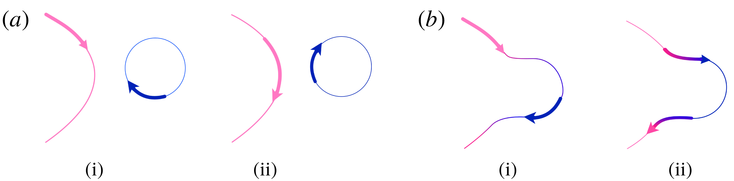
Overall we see that there are two types of interplaying mechanisms, which we sketch in figure 4. The first shows modes approaching with no ‘exchange’ (figure 4 a) and as in the results of figure 2(a). The second does exhibit mode exchange (figure 4 b) as it occurs in the majority of interplaying regions in figure 3(a). These results recall the recent work by Hosseini et al. (Reference Hosseini, Kornilov, Lopez Arteaga, Polifke, Teerling and de Goey2018), in particular, their ‘attachment and detachment’ between ITA and acoustic modes is, in our view, given by an alternating behaviour of the modes. Interestingly, the two types of interplay depicted in figure 4 show that the anti-correlated behaviour of the sensitivities will occur at different locations, depending on the kind of interplay. In the first case, figure 4(a), it occurs when the modes have the same frequency; in the second case, figure 4(b), it occurs when the modes have the same growth rate. We will show in the discussion of the sensitivity results below that the topology of these two types of interplay is linked to the presence of exceptional points.
Sketch (as if the modes are visualised in the complex plane) of the two types of interplay that the modes can exhibit. In the first case (a), the modes approach as shown in panel (i) and the modes approach each other and interplay without exchange (ii). In the second case (b), the modes approach (i) and interplay with exchange (ii). In both cases, the interplay strength depends on the proximity of the eigenvalues to one another.

6.2 Sensitivity analysis
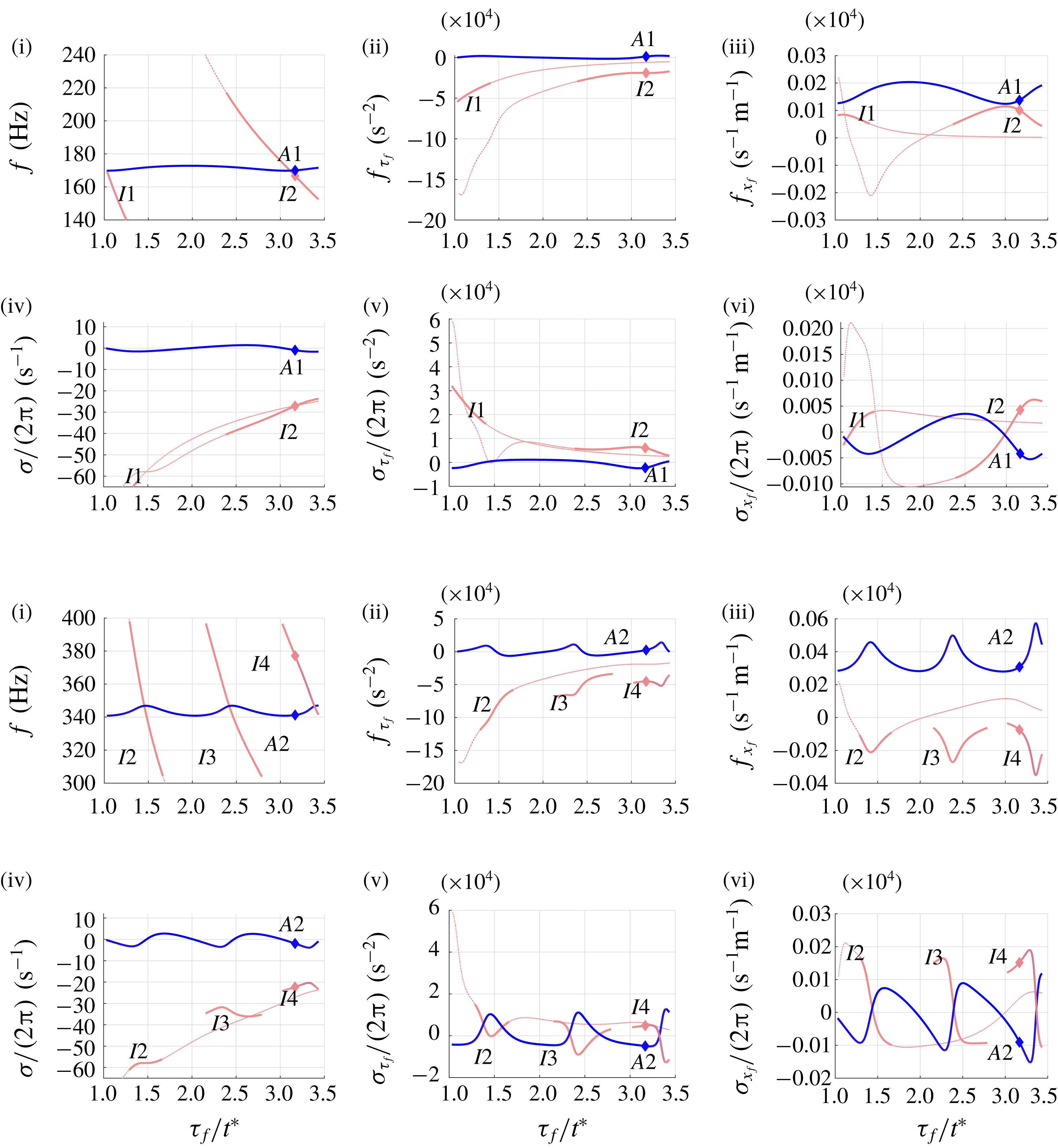
Modal sensitivities at
 $x_{f}=0.48L$
for the first (a) and second (b) acoustic–ITA pairs. Frequencies (i) and growth rates (iv) of the modes are shown for reference. The sensitivities with respect to the flame time delay,
 $f_{\unicode[STIX]{x1D70F}_{f}}$
and
 $\unicode[STIX]{x1D70E}_{\unicode[STIX]{x1D70F}_{f}}/(2\unicode[STIX]{x03C0})$
, are shown in panels (ii, v) and those with respect to the flame location,
 $f_{x_{f}}$
and
 $\unicode[STIX]{x1D70E}_{x_{f}}/(2\unicode[STIX]{x03C0})$
, in panels (iii, vi). Only the full sensitivity curves of ITA modes I1 and I2 are shown as dashed lines, with the interplaying segments in bold. The sensitivities of the other ITA modes are only shown in bold in the relevant interplaying segments. Here
 $\unicode[STIX]{x1D70F}_{f}/t^{\ast }=3.16$
is marked as ♦.

The sensitivities to flame position and flame time delay of both frequency and growth rate for
 $x_{f}=0.48L$
and over the range of time delays investigated are presented in figure 5. In figure 5(a) we show the sensitivities of modes close to the first acoustic frequency (modes A1, I1 and I2), while in figure 5(b) the sensitivities of modes close to the second acoustic frequency (A2, I2, I3 and I4) are displayed. For reference, we also show the frequencies and growth rates versus the flame time delay, respectively, in panels (i) and (iv).
The sensitivities of mode A1 with respect to the flame time delay (
 $f_{\unicode[STIX]{x1D70F}_{f}}$
and
 $\unicode[STIX]{x1D70E}_{\unicode[STIX]{x1D70F}_{f}}$
, respectively, in figures 5
a (ii) and 5
a (v)) show an oscillating behaviour centred around the ordinate axis, in agreement with the Rayleigh criterion. ITA mode I1 clearly shows an inverse proportionality to the flame time delay, while mode I2 deviates from this behaviour around
 $\unicode[STIX]{x1D70F}_{f}/t^{\ast }\approx 3$
and
 $\unicode[STIX]{x1D70F}_{f}/t^{\ast }\approx 1.5$
(the second case is more apparent in figure 5
a (v)). In the first case, the peak of mode I2 corresponds to the interplay with mode A1; in the second case, the mode interplays with mode A2 as can be seen in figure 5
b (iii,v). In order to further highlight this behaviour, we have marked the interplaying segments of each sensitivity curve with a bold line. However, in order to improve the readability of the plots, we keep only these marked segments for the other ITA modes (I3, I4). We stress though that the segments in figure 5(b) are not part of a same line as they belong to the sensitivity curves of different ITA modes, which can be identified by referring to panels (i) and (iv).
The sensitivities with respect to the flame position
 $f_{x_{f}}$
and
 $\unicode[STIX]{x1D70E}_{x_{f}}$
are shown, respectively, in figures 5
a (iii) and 5
a (vi). The sensitivities of A1 show an alternating behaviour. Mode I1 has positive sensitivity with a maximum located at the interplaying region (near
 $\unicode[STIX]{x1D70F}_{f}/t^{\ast }\approx 1$
) before decaying towards zero. Also in this case, mode I2 shows an anti-correlated sensitivity with mode A1 near
 $\unicode[STIX]{x1D70F}_{f}/t^{\ast }\approx 3$
, together with a second region near
 $\unicode[STIX]{x1D70F}_{f}/t^{\ast }\approx 1.5$
anti-correlated with mode A2, as highlighted in figure 5
b (iii,vi).
In general, for the non-exchange type of interplay, the acoustic mode will exhibit sensitivities that oscillate around some constant value, while the ITA modes correlate their sensitivities with those of the acoustic mode they interplay with. The oscillation amplitude of the sensitivities of the acoustic mode and the associated ITA modes is not constant. This is evident in all the sensitivity panels of figure 5(b), where a steepening trend of the sensitivities (e.g. increasingly sharper peaks in figure 5 b (iii)) indicates that the interplay between subsequent ‘crossings’ of ITA modes is becoming stronger as we increase the time delay. This suggests that for increasing flame time delay, the eigenvalue trajectories are closer to the exceptional point associated with the acoustic–ITA pair under consideration. Extremely accurate parameter tuning (beyond the scope of the current model) can lead to the trajectories passing through this point. Further increasing the flame time delay would then result in a change of interplay from the current non-exchange to a mode-exchange type.
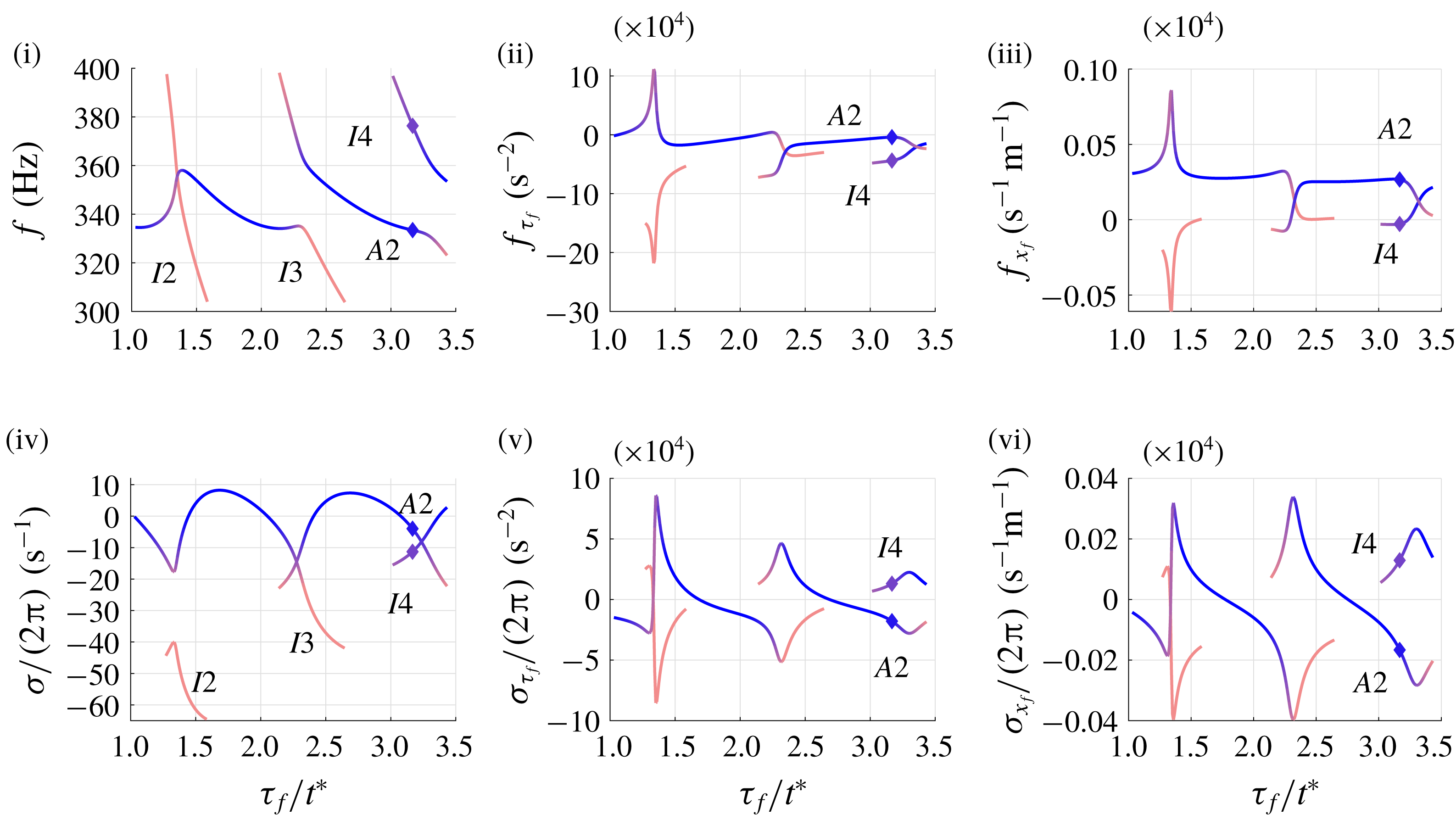
The sensitivities for the case with
 $x_{f}=0.4L$
are shown in figure 6, where only results around the second acoustic frequency are displayed, as the other results are qualitatively similar. The colour coding is based on the classification of either ITA or acoustic modes as in figure 3. Recalling that, as we increase the flame time delay, the interplay is such that different modes will behave as an acoustic mode (see figure 3), we see that their sensitivities reflect this change. Inspecting the sensitivities to the flame time delay (figure 6ii,v), the dark blue segments periodically settle around
 ${\approx}10^{4}~\text{s}^{-2}$
for
 $f_{\unicode[STIX]{x1D70F}_{f}}$
while the growth rates periodically change their sensitivities from a positive to a negative value. These trends are also reflected in the sensitivities with respect to the flame location (figure 6iii–vi) and recollect the trends observed in the non-exchange type in figure 5(b). The periodicity is again dictated by the exchange between the current acoustic mode and the approaching ITA mode and is reflected in the peaks of the sensitivity curves. As observed in figure 5, the strength of the peaks is not constant; rather, larger peaks indicate a proximity to the pertinent exceptional point.
Example of modal sensitivities at
 $x_{f}=0.40L$
for the second acoustic–ITA pair. Frequencies (i) and growth rates (iv) of the modes are shown for reference. The sensitivities with respect to the flame time delay,
 $f_{\unicode[STIX]{x1D70F}_{f}}$
and
 $\unicode[STIX]{x1D70E}_{\unicode[STIX]{x1D70F}_{f}}/(2\unicode[STIX]{x03C0})$
, are shown in panels (ii, v) and those with respect to the flame location,
 $f_{x_{f}}$
and
 $\unicode[STIX]{x1D70E}_{x_{f}}/(2\unicode[STIX]{x03C0})$
, in panels (iii, vi). Only the relevant segments of the sensitivities are plotted as explained in the text. Here
 $\unicode[STIX]{x1D70F}_{f}/t^{\ast }=3.16$
is marked as ♦.

Overall, the results highlight a strong anti-correlated behaviour of the sensitivities (figures 5 and 6) of each acoustic–ITA pair when the modes interplay. This can be intuitively explained by looking at the sketch of figure 4. As the modes approach each other, each will show the sensitivities of its own type. As they interplay, the trajectories in the complex plane follow opposite directions resulting in the anti-correlated behaviour in both frequency and growth rate.
The ‘extreme’ sensitivity (Juniper & Sujith Reference Juniper and Sujith2018) at certain locations is linked to the recent work by Silva et al. (Reference Silva, Yong and Magri2018) and Mensah et al. (Reference Mensah, Magri, Silva, Buschmann and Moeck2018) on exceptional points. The sensitivities of two eigenvalues approaching an exceptional point are expected to increase. Despite our avoiding parameter configurations that give rise to defective eigenvalues (due to limitations of adjoint methods at these exceptional points (Mensah et al. Reference Mensah, Magri, Silva, Buschmann and Moeck2018)), the results show that the effect of exceptional points is nonetheless felt globally. In other words, the presence of exceptional points induces an interplay between modes, influences their trajectories and affects the strength of their parametric sensitivities.
The results are important for optimisation procedures of thermoacoustic systems, which rely on the gradient information of the eigenvalue. Juniper & Sujith (Reference Juniper and Sujith2018) have suggested that the large sensitivities can be used to optimise geometries with very small modifications from the original ones. However, as the interplaying pair has anti-correlated sensitivities, it might be difficult to damp one mode without destabilising others. Of course, if the ITA modes are significantly damped, even large changes will not destabilise the systems, but this might not be the case when the interplay occurs near marginal stability. Furthermore, these results may also explain the evolution of eigenvalues during optimisation studies such as Yang et al. (Reference Yang, Sogaro, Morgans and Schmid2019) where pairs of eigenvalues are seen to present opposite responses to variations in the control parameters.
7 Results: non-modal analysis
We continue our study by focusing on the dynamics of the thermoacoustic problem around parameter combinations that showed strong modal sensitivities. In particular, we will take a non-modal point of view in our analysis. To this end, we locate our flame at
 $x_{f}=0.4679~\text{m}$
and select a flame time delay such that strong sensitivities are encountered for damped, low-frequency modes (
 $f<1000~\text{Hz}$
). In this configuration, higher-frequency unstable modes are present but show a sufficiently small growth rate and thus a negligible influence on our short-time analysis. Moreover, these modes can be discarded on physical grounds as they would be damped under realistic conditions due to acoustic losses in the system as well as a typical low-pass behaviour of real flames (Dowling Reference Dowling1997; Ducruix et al.
Reference Ducruix, Schuller, Durox and Candel2003).
7.1 Angle between acoustic and ITA modes
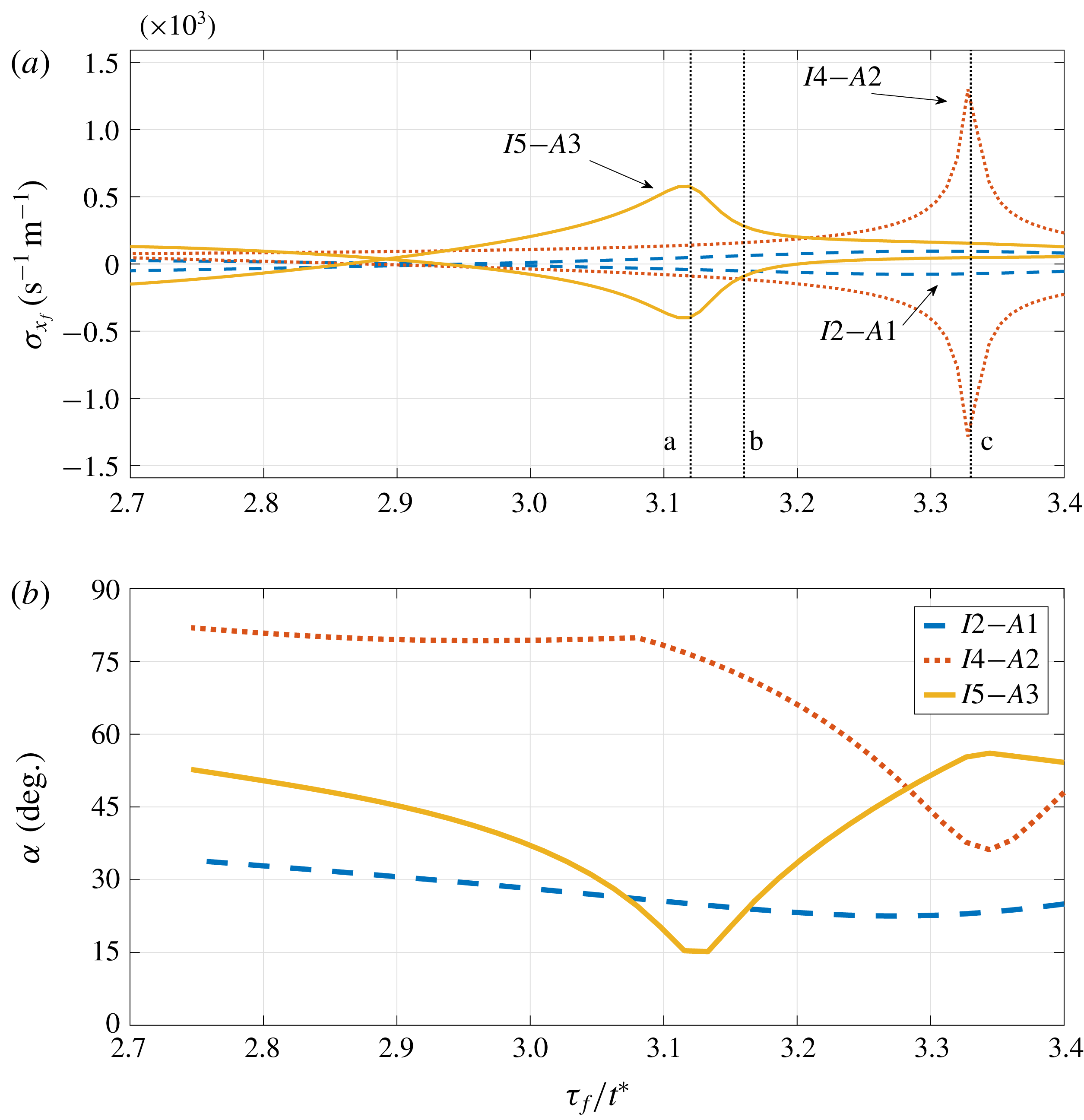
Link between the peak in sensitivities (a) and the angle (b) between selected acoustic–ITA mode pairs. The vertical lines marked as a, b and c correspond, respectively, to the time delays shown in figure 9;
 $\unicode[STIX]{x1D70F}_{f}/t^{\ast }=3.12$
, 3.16 and 3.33.

The marked sensitivity of the acoustic and ITA modes suggests a certain degree of non-normality of the underlying system matrix and, consequently, a noticeable non-orthogonality between the modes. To verify this relation, we investigate the angle between the acoustic and ITA eigenvectors in a narrower range of time delays and juxtapose it to the previous sensitivity results. We evaluate the angles between each one of the first three acoustic modes with every eigenvector in the range (
 $-300\leqslant \unicode[STIX]{x1D70E}\leqslant 50$
,
 $0\leqslant \unicode[STIX]{x1D714}\leqslant 3000\unicode[STIX]{x03C0}$
). The results are shown in figure 7(b) and compared to sensitivity results for the same selection of modes and parameters (see figure 7
a).
A distinct correlation between minima in the angle and regions of strong sensitivity is apparent. This recalls the work by Mensah et al. (Reference Mensah, Magri, Silva, Buschmann and Moeck2018); as the modes approach the exceptional point, the angle between the eigenvectors reduces. At the exceptional point only one eigenvector is found. In our set-up, although the modes never cross at an exceptional point, we also observe the marked decrease in orthogonality between the interplaying modes, corresponding to the region of correlated sensitivities. However, while the eigenvalues of the second acoustic–ITA pair (
 $A2$
–
 $I4$
) exhibit a stronger sensitivity peak, suggesting therefore to be closer to the exceptional point, their non-orthogonality is not as strong as for the first acoustic–ITA pair (
 $A1$
–
 $I2$
). The angle between the second pair (
 $A2$
–
 $I4$
) is not far from being normal (
 ${\approx}80^{\circ }$
) except at the region of interplay, the first pair (
 $A1$
–
 $I2$
) shows an angle that is far from normal (
 ${\approx}30^{\circ }$
) throughout the selected parameter space. The third pair displays intermediate values for the angle, when the modes are far from interplaying.
Overall, we observe a link between the previous sensitivities and the non-normal characteristics of the linear system matrix (expressed as the angle between selected modes). While this finding points towards the presence of non-modal effects, we nonetheless point out that the most non-orthogonal modes do not necessarily correspond to the strongest sensitivity peaks. A more detailed analysis has to reveal the prevalence of non-modal thermoacoustic phenomena in light of acoustic–ITA interplays.
7.2 Pseudospectral analysis
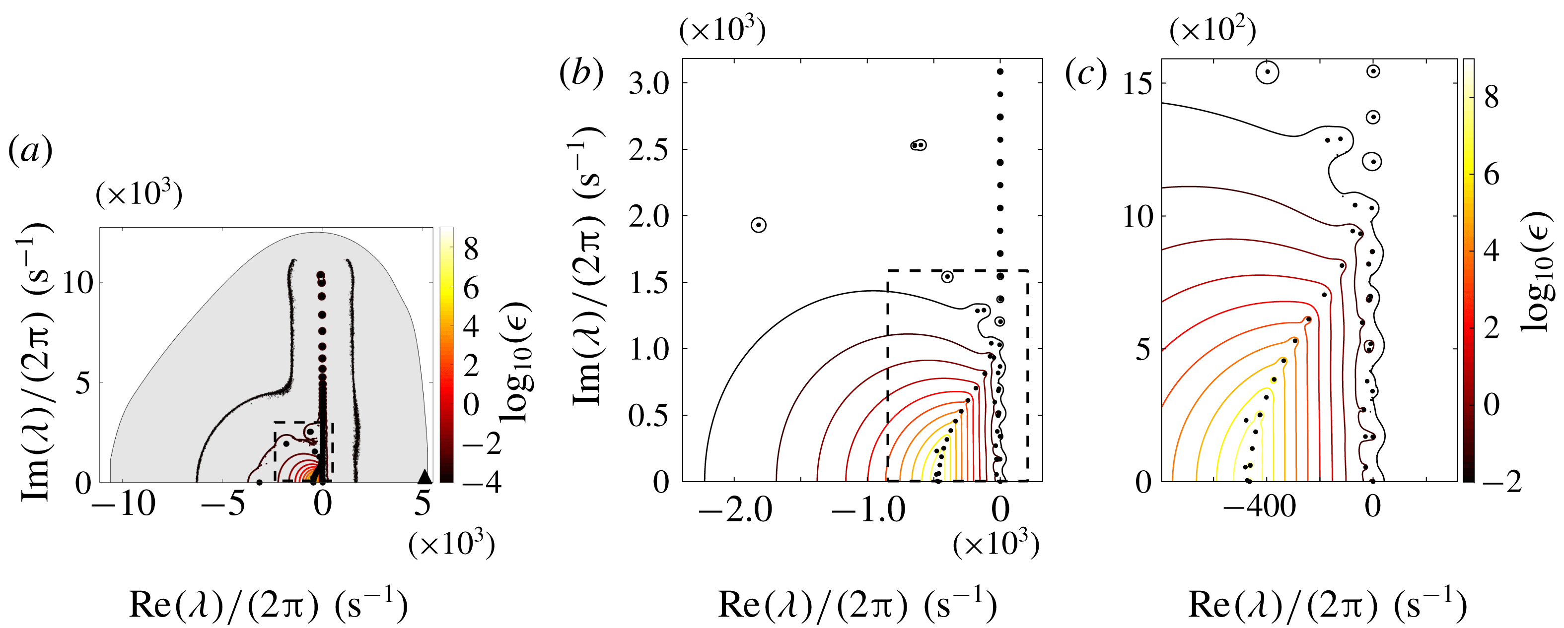
(a) Pseudospectrum (resolvent contours) of the system matrix
 $\unicode[STIX]{x1D63D}$
with superimposed numerical range (grey area), numerical abscissa at
 $3.4\times 10^{4}$
(▴) and spectrum (●) for
 $\unicode[STIX]{x1D70F}_{f}=9.2~\text{ms}$
. Only the upper half of the complex plane is shown as the spectrum is symmetric about the real axis. (b) More detailed view of the area corresponding to the dashed box in (a). (c) More detailed view of the area corresponding to the boxed area in (b).

Pseudospectra (resolvent contours) of the system matrix
 $\unicode[STIX]{x1D63D}$
with logarithmically (
 $\log _{10}$
) spaced contour levels for three different flame time delays. Superimposed is the location of the Kreiss constant (
 $\star$
) for each case.

We proceed with the analysis of the pseudospectra of the system matrix
 $\unicode[STIX]{x1D63D}$
. Figure 8 shows an example of the pseudospectrum, visualised by nested resolvent contours, for the discretised matrix
 $\unicode[STIX]{x1D63D}$
with
 $\unicode[STIX]{x1D70F}_{f}/t^{\ast }=3.16$
. No appreciable qualitative differences can be observed for moderately different flame time delays, and hence only one representative case is shown.
The pseudospectrum confirms the non-normality in the system matrix, with higher contour levels concentrated in the core of the spectrum, around modes that show significant damping. The numerical range (shaded in grey) is included, and the numerical abscissa, i.e. the right-most point of the convex numerical range, is marked by a ▴ symbol. The numerical abscissa is of order
 $O(10^{4})$
, a value that signifies that strong transient effects are particularly fast to occur after
 $t=0$
.
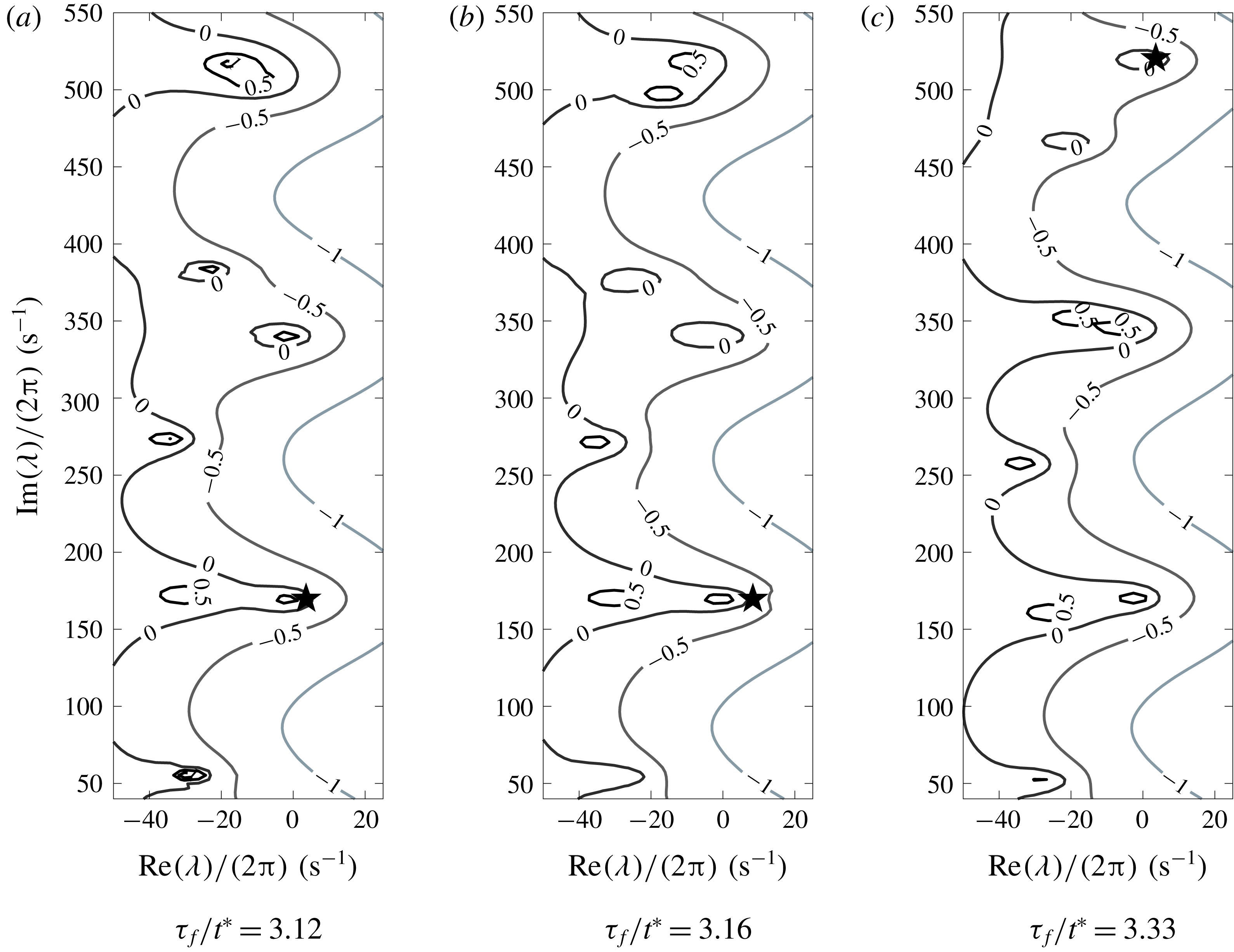
Figure 9 depicts the pseudospectra for
 $\unicode[STIX]{x1D70F}_{f}/t^{\ast }=3.12$
, 3.16 and 3.33 in the low-frequency region near the imaginary axis, focusing on the first three acoustic–ITA pairs, as marked in figure 7(a). In general, little non-normality can be deduced from the pseudospectra, in agreement with previous studies (Magri et al.
Reference Magri, Balasubramanian, Sujith and Juniper2013). However, ITA modes appear to develop more detached resolvent contours (an indication of higher sensitivities) as they interplay with acoustic modes. For example, in the neighbourhood of the third ITA–acoustic pair (near
 ${\approx}530~\text{Hz}$
) the resolvent contour decreases in value from 1 in figure 9(a), to 0.5 in figure 9(b), to 0 in figure 9(c). This decrease in strength correlates with a diminished interplay between the modes. A similar link between an increase of resolvent contour values and an increase in interplay for the second acoustic–ITA pair (at
 ${\approx}330~\text{Hz}$
) is observed in figure 9(b,c), while for the first acoustic–ITA pair the resolvent contours do not change in value, in agreement with the small angle between the respective modes (see the I2–A1 line in figure 7
b).
While the above results do not produce strong evidence for regions of distinct sensitivities, the pseudospectral analysis shows that there is a moderate degree of non-normality in the system, which is further accentuated by the interplay between acoustic and ITA modes. In particular, the Kreiss constant (the computation of the Kreiss constant has been adjusted to the low-frequency region by a subspace projection, as the system matrix contains high-frequency unstable modes) for figure 9(a,b) is located around frequencies that correspond to the first acoustic–ITA pair, suggesting that non-normal effects responsible for transient energy amplification are linked to these particular interplaying modes; this is in agreement with our analysis of the eigenvector angles. This specific pair, while not exhibiting strong sensitivity peaks, is characterised by nearly coalescing frequencies, but markedly different damping rates; the transient energy amplification, however, stems from the non-orthogonality between the involved eigenvectors of the pair. A subspace projection onto various low-frequency modes will shed more light onto the potential for transient energy amplification in our system.
7.3 Transient energy amplification
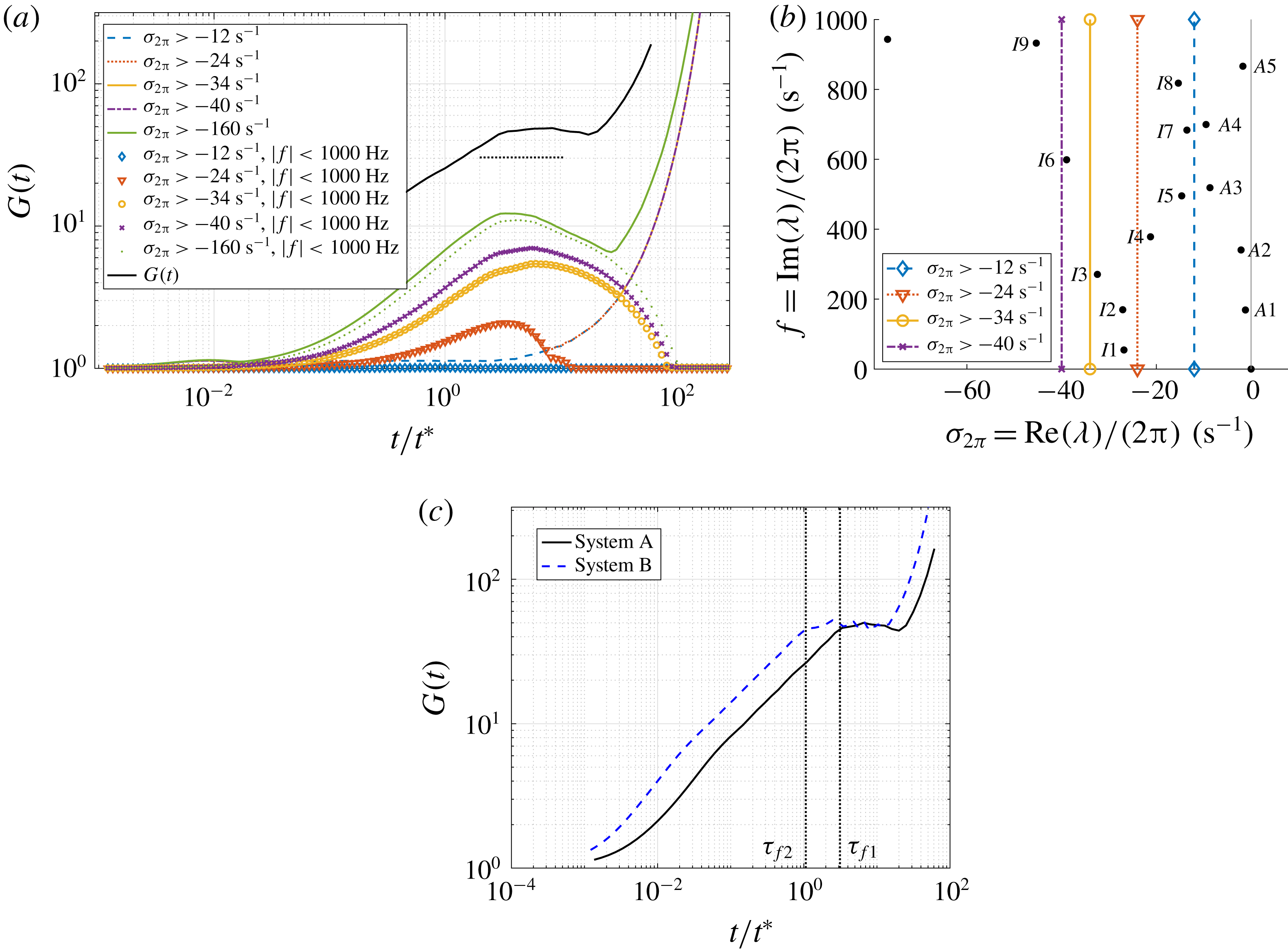
(a) Temporal evolution of the matrix exponential norm
 $G(t)$
(solid black line), together with the evolution of the energy norm for selected modal projections (coloured lines identify different projections based only on growth rate; symbols identify projections in which both growth rate and frequency have been used to select the modal subspace). The dotted horizontal line shows the estimate of maximum transient growth based on the Kreiss constant. (b) Spectrum indicating the selected subspaces for (a). (c) Comparison of
 $G(t)$
for the same system with different flame time delays (system A with
 $\unicode[STIX]{x1D70F}_{f1}/t^{\ast }=3.16$
, system B with
 $\unicode[STIX]{x1D70F}_{f2}/t^{\ast }=1.1$
). The vertical lines indicate the two flame time scales.

The calculation of the maximum energy amplification
 $G(t)$
follows the procedure outlined in § 4, and it is shown as a black solid line in figure 10(a), for the case
 $\unicode[STIX]{x1D70F}_{f}/t^{\ast }=3.16$
. We observe transient growth of
 $O(10)$
, before the unstable high-frequency modes dominate the dynamics at longer time scales. This magnitude is in accordance with the lower bound estimated by the Kreiss constant (obtained by applying (5.5) to the value shown in figure 9
b), indicated in figure 10(a) as a horizontal dashed line. The transient growth found is larger than reported in previous studies (Juniper Reference Juniper2011; Mariappan et al.
Reference Mariappan, Sujith and Schmid2011; Magri et al.
Reference Magri, Balasubramanian, Sujith and Juniper2013; Blumenthal et al.
Reference Blumenthal, Tangirala, Sujith and Polifke2017); this is a direct consequence of our choice of integrating the acoustic energy over a period of time equivalent to
 $\unicode[STIX]{x1D70F}_{f}$
.
Transient growth effects develop over a time scale comparable with the flame time delay: two different cases of
 $\unicode[STIX]{x1D70F}_{f1}/t^{\ast }=3.16$
and
 $\unicode[STIX]{x1D70F}_{f2}/t^{\ast }=1.1$
are included in figure 10(c). This finding is consistent with the form of the equations, as information is linearly advected from the past over an interval
 $\unicode[STIX]{x1D70F}_{f}$
. It suggests that the flame itself (via its delayed heat release) contains potential for transient energy amplification.
To further investigate this point, we project the system matrix onto a subspace spanned by a selection of eigenvectors (see Schmid Reference Schmid2007) to assess the contribution of specific modes to overall transient effects. We include the results in figure 10(a) selecting reduced bases with increasingly smaller growth rates. In particular, the first case (
 $\text{Re}(\unicode[STIX]{x1D706})/2\unicode[STIX]{x03C0}>-12~\text{s}^{-1}$
) contains only acoustic modes, and we observe no transient effects at all. Expanding the subspace to include the least damped ITA modes (
 $\text{Re}(\unicode[STIX]{x1D706})/2\unicode[STIX]{x03C0}>-24~\text{s}^{-1}$
) is sufficient for transient growth to arise with energy gains of
 ${\sim}2$
. Including all ITA modes yields amplifications of
 ${\sim}5$
. We further investigate the effects of excluding higher-frequency modes (i.e. modes with
 $|f|<1000~\text{Hz}$
) and note that the transient dynamics is identical.
This suggests that the presence of ITA modes leads to transient energy gains comparable to or slightly larger than those found in previous studies (Zhao Reference Zhao2012; Magri et al. Reference Magri, Balasubramanian, Sujith and Juniper2013; Mariappan et al. Reference Mariappan, Sujith and Schmid2015). Moreover, for all investigated subspace projections, the time scale for transient growth coincides with the flame time response. This mechanism permits a two-component scenario where transient energy amplification occurs over a first (short) time scale before it feeds, in a second step, the normal, acoustic dynamics. The presence and interplay of acoustic and ITA modes are sufficient for this mechanism to be viable and observable.
7.4 Optimal initial conditions
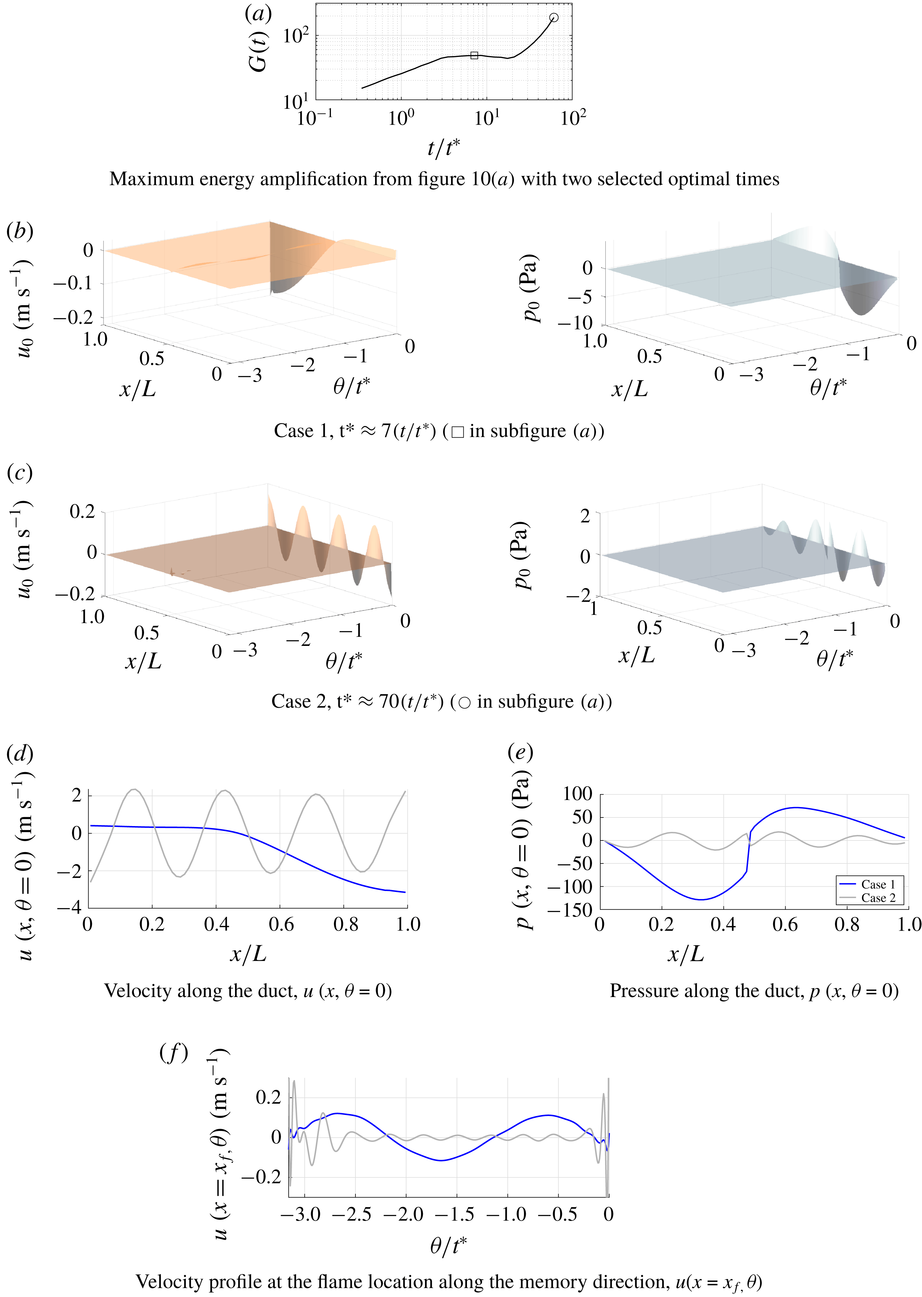
Comparison of two optimal initial conditions. Case 1: optimal initial condition for transient growth (▫). Case 2: optimal initial condition for normal long-time dynamics (○). (a) Maximum energy growth, reproduced from figure 10(a), with the two different optimal times. (b,c) Velocity (left) and pressure (right) of the two optimal initial conditions in both space and memory dimension. Comparison of (d) the velocity and (e) the pressure components of the two initial conditions along the tube (
 $u(x,\unicode[STIX]{x1D703}=0)$
,
 $p(x,\unicode[STIX]{x1D703}=0)$
). (f) Comparison of the velocity signal of the two initial conditions along the memory dimension at the flame location
 $(u(x=x_{f},\unicode[STIX]{x1D703}))$
.

Besides assessing the maximum energy amplification by non-modal effects in thermoacoustic systems, we are also interested in the shape of the particular initial condition that triggers this optimal growth in energy. A similar analysis has been reported in Juniper (Reference Juniper2011) and Blumenthal et al. (Reference Blumenthal, Tangirala, Sujith and Polifke2017). However, owing to the present discretisation of the delay-differential system, we also allow degrees of freedom related to the time delay of the flame model. The initial conditions have been obtained from a singular value decomposition of the matrix exponential; the resulting principal vector is multiplied by
 $\unicode[STIX]{x1D652}^{-1}$
to obtain the optimal pressure and velocity shapes.
Two selected times, concentrating on short- and long-time behaviour, for which initial conditions are to be computed are shown in figure 11(a) superimposed on the maximum growth curve
 $G(t)$
. The resulting initial conditions are depicted in figure 11(b,c). The figure shows the shape of the optimal initial condition in the domain (along the tube as well as along the memory coordinate). Figure 11(b) corresponds to the optimal initial condition that is subject to transient growth, as its optimal time falls within the algebraic amplification period of
 $G(t)$
. The associated shapes of the optimal initial conditions unveil a small-amplitude ridge along the memory coordinate aligned with the flame location
 $x_{f}$
(this is better visualised in figure 11
f, described below), and attached to a modal shape at zero time delay. Other initial conditions (not shown) obtained in the transient optimal time range (
 $\unicode[STIX]{x1D70F}_{f}/t^{\ast }<t/t^{\ast }<10$
) exhibit slightly different spatial modal shapes at zero time delay, but show no qualitative difference in the ridge structure from the one shown in figure 11(b). The presence of the ridge in the memory dimension corresponding to the velocity node placed at the flame location is not surprising, as the flame model is only aware of time-lagged values of this quantity.
The distributions of the memory signal can be compared for the two cases of optimal initial conditions for transient growth and for long-time dynamics to give insight into the mechanism of transient amplification.
The important features of the two different optimal initial conditions are compared in figure 11(d–f). The spatial velocity and pressure distributions along the tube and for the instantaneous time
 $\unicode[STIX]{x1D703}=0$
, respectively
 $u(x,\unicode[STIX]{x1D703}=0)$
and
 $p(x,\unicode[STIX]{x1D703}=0)$
, are compared in figure 11(d,e). The optimal initial condition for the long-time dynamics (case 2) clearly shows the seventh acoustic mode shape, corresponding to the unstable frequency of
 ${\approx}1200~\text{Hz}$
. The comparison of the distribution of the velocity in the memory dimension (
 $u(x=x_{f},\unicode[STIX]{x1D703})$
) is shown in figure 11(f). For case 1, the period of excitation along the memory direction is consistent with the first acoustic mode
 $(2t^{\ast })$
. For case 2, the period of excitation is approximately
 $t^{\ast }/3$
, with a lower amplitude. The above described shapes of the optimal initial conditions for transient and long-time dynamics have also been investigated when the norm is such that only the instantaneous acoustic energy is considered. This was done to ensure that the results are independent of the choice of norm, as highlighted by Blumenthal et al. (Reference Blumenthal, Tangirala, Sujith and Polifke2017). The results showed no qualitative differences from those described above.
7.5 Evolution of the optimal initial condition and transient growth mechanism
Further insight into the mechanism of transient growth for the current system can be gained by analysing the evolution in time of the product between the pressure at the flame location,
 $p(x_{f},t)$
, and the time-lagged velocity at the flame location,
 $u(x_{f},t-\unicode[STIX]{x1D70F}_{f})$
. As this latter term is directly proportional to the unsteady heat release rate (equation (4.1)), the product acts as a surrogate for the argument in the Rayleigh-criterion integral (
 $\int _{T}p^{\prime }q^{\prime }\,\text{d}t$
). We have plotted this quantity for the two cases in figure 12. It can be clearly seen that during the first flame time-delay cycle (its duration is indicated by the vertical dashed line) the initial condition for transient growth is such that the product is always positive. Indeed, the memory signal of the lagged velocity is always in phase with the pressure evolution of the first acoustic mode. After the first cycle of the time delay, the memory signal of the velocity at the flame location has been replaced by the evolving one, and therefore it is no longer optimal, resulting in the product oscillating between positive and negative values. The amplitudes are seen to decay. The large amplitude of the first oscillation immediately after the first time-delay cycle indicates that the energy gained by the system is large.
On the other hand, case 2 shows that the product remains mainly positive throughout the simulation, and the oscillations grow in time. Furthermore, there is no significant change in amplitudes between the oscillations before and after the first time-delay cycle. The results recall those presented in Blumenthal et al. (Reference Blumenthal, Tangirala, Sujith and Polifke2017). The mechanism of excitation relies on a Rayleigh-like source term. However, contrary to their results, the distribution of the flame velocity in the memory direction is key in transient amplification.
The above results suggest that the degrees of freedom related to the time delay of the problem are of significant importance in the transient-growth analysis and that a particular excitation at the flame location can produce noticeable energy gains. Furthermore, the short-time dynamics of our system is governed by the excitation at the flame over the course of the time delay, in agreement with Blumenthal et al. (Reference Blumenthal, Tangirala, Sujith and Polifke2017), while the long-time dynamics is independent of the flame element and predominantly acoustic in nature.
Evolution of the product between the pressure perturbation at the flame location
 $p(x_{f},t)$
and the delayed value of the velocity at the flame
 $u(x_{f},t-\unicode[STIX]{x1D70F}_{f})$
. The dashed vertical line indicates the first complete flame time-delay cycle. Case 1 corresponds to an initial condition subject to transient growth (indicated with ▫ in figure 11
a). Case 2 corresponds to an initial condition with no transient growth (indicated with ○ in figure 11
a).

The link between transient dynamics and the presence of ITA modes is, however, more subtle. Our results show that, while the non-orthogonality between the two types of modes is correlated to appreciable sensitivities, transient effects show no such link. In fact, the pseudospectral and Kreiss-constant results have shown that a proximity to the imaginary axis of either mode of an acoustic–ITA pair with similar frequencies is more important. For these cases, the pair was composed of a slightly damped acoustic mode and a significantly damped ITA mode with similar frequency; in addition, the angle between the modes was small, but no substantial sensitivities were found. In summary, within the limitations of our simplified thermoacoustic system, transient effects with amplification factors between two and five occur, once both acoustic and ITA modes are included in the analysis.
8 Conclusions
We have considered a simplified version of a horizontal Rijke tube as a quintessential example of thermoacoustic instability. Our focus was a study of the system’s dynamics for parameter configurations that induce strong modal sensitivities. These configurations are encountered when acoustic modes, which are typically related to the geometric shape of the combustion chamber, interplay with ITA modes.
Varying the flame time delay and the flame location, we observe pairs of eigenvalues, consisting of one acoustic mode and one ITA mode, that approach each other and may exchange type. This interplay is reflected in pronounced modal sensitivities which become increasingly larger as the two modes approach each other in the complex plane.
Changing to a dynamical-system representation of the problem, a non-modal stability approach has been chosen based on non-orthogonality arguments, pseudospectra, Kreiss-constant estimates, numerical abscissas, transient growth computations and optimal initial conditions. While a correlation between a diminishing angle between acoustic and ITA modes and parametric regions of high modal sensitivities could be established, transient growth effects did not follow the same correlation. An analysis of the pseudospectra of the system matrix revealed that the proximity to the imaginary axis of only one of the modes in an acoustic–ITA pair is a sufficient factor for transient growth, which is also captured by the location of the Kreiss constant in the complex plane. Stronger sensitivities are caused by an interplay between the third acoustic–ITA modal pair. While the pseudospectral contours appear extended around this interplaying pair, the location in a highly damped region of the complex plane severely limits any contributions to transient growth. In contrast, despite showing small modal sensitivity, the acoustic mode of the first acoustic–ITA pair is close to the imaginary axis, the angle between the two modes is rather small and the pseudospectral contours protrude visibly into the unstable half-plane. The Kreiss constant, providing a lower bound on the maximum transient growth, is consequently linked to this pair of modes.
An analysis of the matrix exponential norm confirms amplification factors of order
 $O(10)$
over short time scales, corroborated by a substantial numerical abscissa. Using projections on reduced subspaces (spanned by selected modes), the various contributions to the overall transient amplification have been identified: while a purely acoustic basis yielded no transient growth, the inclusion of ITA modes produced transient energy gains similar to previous studies. Furthermore, a change in the flame time delay induced a commensurate change in the time that the maximum energy gain is reached. This finding identifies the flame component of the Rijke tube as a potential transient amplifier, acting over one flame time scale. This is further supported by studying the optimal initial condition: a perturbation in the velocity component concentrated at the flame location and acting over the duration of the flame time delay has been found responsible for the maximum energy gain due to non-modal effects. Modal effects (without significant transient growth) are dominated by purely acoustic perturbations and govern the long-time dynamics of the system.
Overall, the pivotal role of ITA modes in the analysis and design of thermoacoustic systems has been demonstrated. The flame component, and its interplay with the acoustic structures of the combustion chamber, has been identified as the main contributor to transient energy amplification. As such, it contributes directly to thermoacoustic instabilities and indirectly to the triggering of finite-amplitude limit-cycle behaviour.
Acknowledgements
The authors are grateful for the funding provided by the EPSRC Centre for Doctoral Training (CDT) in Fluids Mechanics Across Scales, the Department of Mathematics at Imperial College London and the Department of Mechanical Engineering at Imperial College London.
Supplementary movies
Supplementary movies are available at https://doi.org/10.1017/jfm.2019.632.