1. Introduction
The theory of laminar flames and associated activation-energy asymptotics (Buckmaster & Ludford Reference Buckmaster and Ludford1982; Williams Reference Williams1985; Zel’dovich et al. Reference Zel’dovich, Barenblatt, Librovich and Makhviladze1985), which provides a precise description of premixed flame structures, is based on the strong nonlinearity of chemical reactions. As a result of this highly nonlinear behaviour, the flame structure features two distinct zones with markedly different characteristic scales: a preheat zone, corresponding to an equilibrium between convection and diffusion of chemical species and heat, and a reaction zone characterized by an equilibrium between molecular diffusion and reaction processes. An essential characteristic of activation-energy asymptotics (AEA) is to restrict the dimensions of the region in which chemical reaction is significant.
This flame theory cannot be readily extended to the consideration of turbulent reactive flows (Liñán & Williams Reference Liñán and Williams1993). The complexity of the physical mechanisms involved in turbulent flames indeed requires the introduction of many ad hoc simplifications which restrict the development of their theoretical analyses as well as the extension of flame theory to turbulent combustion. As a consequence, the description of the turbulent flame structures remains essentially based on phenomenological grounds. For instance, the different regimes of turbulent premixed combustion are identified from a direct comparison between turbulence and chemistry characteristic length and time scales (Borghi Reference Borghi1984, Reference Borghi and Casci1985; Peters Reference Peters1986). More recently, direct numerical simulation (DNS) studies have shed some light on the phenomenology of flame–turbulence interactions, and the most recent research efforts concern the analysis of the interaction of high-speed turbulence with flames (Poludnenko & Oran Reference Poludnenko and Oran2010) or combustion regimes associated with large values of the Karlovitz number (Savre, Carlsson & Bai Reference Savre, Carlsson and Bai2013) as well as the transition to the distributed burning regime (Aspden, Day & Bell Reference Aspden, Day and Bell2011). However, one of the most studied regimes of turbulent premixed combustion remains the so-called flamelet regime that corresponds to very small values of the (laminar) flame characteristic scales in comparison with the turbulence characteristic scales, i.e. situations featuring high Damköhler number. In this limit the flame brush is considered to be composed of local laminar flame elements (flamelets) convected by the turbulent motions. The corresponding regime of turbulent premixed combustion undoubtedly remains the best suited to perform theoretical analyses of turbulent combustion, such as those early performed by Clavin & Williams (Reference Clavin and Williams1979), Bray et al. (Reference Bray, Libby, Masuya and Moss1981) and Libby & Bray (Reference Libby and Bray1981). In this regime, based on the early works of Kolmogorov, Petrovskii & Piskunov (Reference Kolmogorov, Petrovskii and Piskunov1937), it has been shown that the propagation of the turbulent flame brush is mainly controlled by the phenomena involved at its leading edge (pulled waves). The leading edge is subject to strong modifications in the turbulent transport processes in the form of a transition from a classical gradient-like diffusion mechanism to a countergradient or segregation mechanism, which is associated with flame surface displacements under the influence of laminar flamelet propagation and thermal expansion effects (Bray et al. Reference Bray, Libby, Masuya and Moss1981; Libby & Bray Reference Libby and Bray1981; Robin, Mura & Champion Reference Robin, Mura and Champion2011). As evidenced from both direct numerical simulation studies (Rutland & Cant Reference Rutland and Cant1994; Veynante et al. Reference Veynante, Trouvé, Bray and Mantel1997; Robin et al. Reference Robin, Mura, Champion and Hasegawa2010, Reference Robin, Mura and Champion2011) and experimental investigations, see for instance Kalt, Chen & Bilger (Reference Kalt, Chen and Bilger2002), the corresponding transition takes place throughout a very thin region of the turbulent flame brush located in the vicinity of the leading edge, which emphasizes the crucial need for its accurate description. In this respect travelling wave analyses have been recently extended to generalized, i.e. non-gradient, closures of the turbulent transport, exhibiting a possible transition from pulled to pushed waves due to countergradient transport (Sabel’nikov & Lipatnikov Reference Sabel’nikov and Lipatnikov2013). Accordingly, the objective of the present study is to propose a refined analysis of the leading edge of the turbulent flame brush, in a manner quite similar to the one retained within the AEA framework. This leads to a description of the different layers that compose its internal structure. The dominant physical mechanisms involved in each of these layers can be identified and their respective characteristic thickness evaluated. The evolution of the scalar fluctuations through the different sublayers is also studied analytically via the segregation rate evolution, a key parameter in models for the mean chemical rate and turbulent transport terms, which also reflects the presence of flamelets when approaching unity. The examination of DNS databases shows that this segregation rate decreases on both sides of the turbulent flame brush (Mura, Tsuboi & Hasegawa Reference Mura, Tsuboi and Hasegawa2008), which provides an additional argument in favour of a refined analysis of the influence of flame brush edges so as to understand how bimodality and associated large-Damköhler-number conditions are reached within the flamelet regime of turbulent premixed combustion.
This manuscript is organized as follows: § 2 introduces the physical concepts and characteristic length and time scales. In § 3, the most important results of the thin flamelet statistical description are summarized before extending it to be valid at the boundaries of the turbulent flame brush where the influence of laminar flame finite thickness becomes non-negligible. Finally, the manuscript ends with a new and detailed analysis of the entire structure of the turbulent flame brush, where an analytical description of the progress variable segregation rate evolution is provided.
2. Flamelet characteristic scales
2.1. Laminar flamelets versus turbulent flamelet elements
The whole description of the turbulent flames proposed in the present study assumes that the local flame structure can be represented by laminar flame elements. These laminar flame elements, hereafter denoted by finite thickness flamelets, are characterized by their own length scale
 $l_{x}$
, which can differ from the thickness of the freely propagating laminar flame
 $l_{f}$
. The introduction of this specific length scale
 $l_{x}$
modifies neither the phenomenology of the flame–turbulence interaction involved in the wrinkled flames regime, nor the results of the associated Bray–Moss–Libby (BML) theory (Bray & Libby Reference Bray, Libby, Libby and Williams1994). However, as shown below, it is an intermediate step before the subsequent investigation of the behaviour of flame brush boundaries, which constitutes one objective of this study. It may also be thought as a first step towards an unified characterization of the turbulent premixed combustion regimes. Before setting more precisely the definition of such finite thickness flamelets, we now proceed by recalling well-known characteristics of both the laminar flame structure and turbulent premixed combustion regimes.
We use a progress variable
 $c$
, defined to be zero (
 $c\equiv 0$
) in the fresh reactants and unity (
 $c\equiv 1$
) in the fully burnt products. Accordingly, under the low-Mach-number approximation, the equation of state reduces to
 ${\it\rho}={\it\rho}_{u}/(1+{\it\tau}c)$
, where
 ${\it\tau}={\it\rho}_{u}/{\it\rho}_{b}-1$
denotes the expansion factor, with
 ${\it\rho}_{u}$
and
 ${\it\rho}_{b}$
the density in the fresh reactants and combustion products respectively. In a first step of the analysis, let us consider a single-step reaction mechanism of the form R (reactants)
 $\rightarrow$
P (products), where the reaction rate is given by an Arrhenius expression
 ${\it\omega}_{Y_{R}}=B{\it\rho}Y_{R}\exp (-T_{a}/T)$
with activation temperature
 $T_{a}$
and mass fraction of reactant
 $Y_{R}$
. It is convenient to follow Williams (Reference Williams1985) and cast this expression into the following form
 $$\begin{eqnarray}{\it\omega}_{c}=\mathscr{B}\frac{{\it\rho}_{u}(1-c)}{(1+{\it\tau}c)}\exp \left(-\frac{{\it\beta}(1-c)}{1-{\it\alpha}(1-c)}\right)\end{eqnarray}$$
which corresponds to the rate of production of the progress variable
 $c$
. In this expression, the quantity
 $\mathscr{B}=B\exp (-{\it\beta}/{\it\alpha})$
is the reduced pre-exponential factor,
 ${\it\alpha}=(T_{b}-T_{u})/T_{b}$
denotes the temperature factor, with
 $T_{u}$
and
 $T_{b}$
the temperature of fresh reactants and fully burned gases respectively, and
 ${\it\beta}={\it\alpha}T_{a}/T_{b}$
is the Zel’dovich number. The structure of such premixed laminar flames has been analysed for large values of the Zel’dovich number
 ${\it\beta}$
, see for instance Clavin (Reference Clavin1985). In this case, the chemical reaction rate
 ${\it\omega}_{c}$
can be considered as exponentially small in the major part of the flow except at the trailing edge of the premixed flame front, where the value of the progress variable approaches unity. Thus, a preheat zone where heat diffuses towards fresh reactants, followed by a thin reaction zone on the hot gas side, are identified. In the limit of infinitely large values of
 ${\it\beta}$
, the thickness of this reaction zone, i.e.
 $l_{R}$
, becomes vanishingly small in comparison with the thickness of the preheat zone, so that the thickness of the latter is approximately equal to the flame thickness
 $l_{f}$
.
To analyse the structure of the premixed flame, it is expedient to adopt a coordinate system attached to the flame. The flow is thus steady, planar, and one-dimensional in the retained frame of reference. The preheat zone is characterized by an equilibrium between convection and diffusion, and the progress variable transport equation reduces to:
 $$\begin{eqnarray}{\it\rho}_{u}u_{f}\frac{\text{d}c}{\text{d}x}=\frac{\text{d}}{\text{d}x}\left({\it\rho}D\frac{\text{d}c}{\text{d}x}\right),\end{eqnarray}$$
where
 $u_{f}$
is the laminar flame propagation velocity and
 $D$
denotes the molecular diffusion coefficient. (Note that for the sake of conciseness and simplicity, Lewis and Schmidt number effects have been discarded from the present analysis.) In the preheat zone, the variations of
 ${\it\rho}D$
are neglected only for the sake of simplicity and the non-dimensional form of (2.2) reduces to:
 $$\begin{eqnarray}\text{d}c/\text{d}x^{\ast }=c,\end{eqnarray}$$
where
 $x^{\ast }=x/l_{f}$
. The progress variable evolution
 $c(x)$
is thus found to be exponential from the fresh gases side at
 $x\rightarrow -\infty$
(
 $c=0$
), where it is governed by molecular diffusion, to the fully burnt gases at
 $x\rightarrow 0$
(
 $c\rightarrow 1$
), where chemical reactions occur. The progress variable thus varies over an infinite distance and the quantity
 $l_{f}$
characterizes the thickness associated with its significant variations across the flame front, as such the laminar flame thickness is often deduced from the highest values of the scalar gradient. This allows one to depict the corresponding characteristic length scale from the tangent to
 $c(x)$
at the position of the maximum scalar gradient. In the limit of large values of the Zel’dovich number
 ${\it\beta}$
the location of this maximum corresponds to
 $c\rightarrow 1$
. In this case, over the characteristic distance
 $l_{f}$
, the progress variable varies from
 $c_{l_{f}}=\exp (-1)$
, which is a non-negligible value, to unity, and the progress variable variations become negligible, i.e. of the order of one percent, at a distance from the reaction zone, which is approximately five times larger than
 $l_{f}$
. The definition of the characteristic thickness of the laminar flame
 $l_{f}$
yields the characteristic time scale of the laminar flame:
 $t_{f}=l_{f}/u_{f}$
. It is noteworthy that, from a detailed description of chemistry and molecular transport, see for instance Ern & Giovangigli (Reference Ern and Giovangigli1995), other definitions involving intermediate species could be retained for the flame thickness
 $l_{f}$
.
Once the characteristic length and time scales of the laminar premixed flame structure,
 $l_{f}$
and
 $t_{f}$
, are defined, a comparison with their turbulence counterparts, i.e. the integral scales (
 $l_{t}$
,
 $t_{t}$
) and the Kolmogorov scales (
 $l_{{\it\eta}_{K}}$
,
 $t_{{\it\eta}_{K}}$
) can be performed. In this respect the Taylor length scale has been also recently shown to be an essential ingredient to describe the interaction between combustion and turbulence at the smallest scales (Mura & Champion Reference Mura and Champion2009). Such comparisons are at the basis of the construction of turbulent premixed combustion diagrams (Barrère Reference Barrère1974; Borghi Reference Borghi1984, Reference Borghi and Casci1985; Williams Reference Williams1985; Peters Reference Peters1986, Reference Peters1999; Pope Reference Pope1987) with a relationship between the structure and the propagation of turbulent premixed flames emphasized in the early studies of Damköhler (Reference Damköhler1947). The corresponding characteristic velocities are respectively denoted
 $u_{f}$
,
 $u_{RMS}=l_{t}/t_{t}$
and
 $u_{{\it\eta}_{K}}=l_{{\it\eta}_{K}}/t_{{\it\eta}_{K}}$
, with the root mean square velocity fluctuations, i.e.
 $u_{RMS}$
, readily deduced from the turbulence kinetic energy
 $\widetilde{k}$
. Moreover, in the following,
 $\widetilde{{\it\Phi}}$
denotes the Favre-averaged value of any quantity
 ${\it\Phi}$
, while
 ${\it\Phi}^{\prime \prime }={\it\Phi}-\widetilde{{\it\Phi}}$
is the corresponding fluctuation. The smallest scales of the turbulent flow field are associated with molecular processes induced by viscous effects, so that
 $l_{{\it\eta}_{K}}={\it\nu}/u_{{\it\eta}_{K}}$
, with
 ${\it\nu}$
the molecular viscosity, and
 $Re_{{\it\eta}_{K}}=1$
. These viscous processes are similar in many respects to the molecular diffusion mechanisms that occur in the premixed laminar flame front, which is also characterized by a flame Reynolds number
 $Re_{f}$
approximately equal to unity. Following the classical K41 description of turbulence (Kolmogorov Reference Kolmogorov1941), the turbulent scales can be related to the turbulent kinetic energy
 $\widetilde{k}$
and its dissipation rate
 $\widetilde{{\it\epsilon}}$
, thus leading to
 $t_{t}=\widetilde{k}/\widetilde{{\it\epsilon}}$
,
 $l_{t}=\widetilde{k}^{3/2}/\widetilde{{\it\epsilon}}$
,
 $t_{{\it\eta}}=({\it\nu}/\widetilde{{\it\epsilon}})^{1/2}$
and
 $l_{{\it\eta}_{K}}=({\it\nu}^{3}/\widetilde{{\it\epsilon}})^{1/4}$
(Tennekes & Lumley Reference Tennekes and Lumley1972). This also provides the definitions of the following classical non-dimensional numbers: (i) the turbulence Reynolds number
 $Re_{t}=u_{RMS}l_{t}/{\it\nu}=(t_{t}/t_{{\it\eta}})^{2}$
, which compares the turbulence integral scale to the Kolmogorov scale, (ii) the Damköhler number
 $Da=t_{t}/t_{f}$
, which compares the turbulence integral scale to the laminar premixed flame characteristic scale, and (iii) the Karlovitz number
 $Ka=t_{f}/t_{{\it\eta}_{K}}$
, which compares the laminar premixed flame characteristic scale to the Kolmogorov scale. Accordingly, these numbers are interrelated:
 $Re_{t}=Da^{2}Ka^{2}$
. In the following we will concentrate on departures from the flamelet regime at the flame brush edges, with
 $Re_{t}$
and
 $Ka$
retained as the two independent parameters. Indeed the Karlovitz number appears as the relevant parameter to analyse the small-scale turbulence–flame interactions. Discarding the possible influence of non-unity Schmidt number effects, the Karlovitz number may be also expressed as the ratio of laminar flame to Kolmogorov length scales, i.e.
 $Ka=t_{f}/t_{{\it\eta}}=(l_{f}/l_{{\it\eta}_{K}})^{2}$
. The present study is conducted under the assumption of finite but sufficiently large values of both Reynolds and Damköhler numbers so as to enforce a scale separation argument between the integral scales and the smallest scales of the flow where molecular mechanisms, i.e. viscous processes, molecular diffusion and chemical reactions, take place. The focus is placed on the effects of finite values of the Karlovitz number. Following the early analyses of Klimov (Reference Klimov1963) and Williams (Reference Williams1976) the corresponding limit, which is given by
 $Ka$
sufficiently larger than unity, is indeed standardly retained to define the upper boundary of the wrinkled (or corrugated) flamelet regime of turbulent combustion. Above this limit, the influence of the turbulent flow field on the local flame structures may become non-negligible and may no longer be reduced to slight modifications of local flamelet propagation velocity through strain and curvature effects. In the following, the Karlovitz number will be used to define precisely the characteristic thickness of flamelets.
In the wrinkled flames regime, it is considered that the inner structure of laminar flames is not altered by turbulent eddies, the influence of which is restricted to strain and curvature effects. Accordingly, laminar flamelet structures are retained as a common building block of many turbulent combustion representations. Such flamelet representations imply that, at the smallest scales of the turbulent flow, the molecular processes involved in flames, i.e. molecular diffusion and chemical reactions, are the dominant processes. The characteristic length scale of these laminar-like flamelet structures is standardly considered to be
 $l_{f}$
. As far as turbulent reacting flows are concerned, the laminar flame thickness
 $l_{f}$
is required to delineate a priori the regimes of turbulent combustion. However, this quantity does not provide any information about the real thickness of flamelets present in the turbulent flows and may not be relevant to characterize it. Therefore it is chosen here to define the flamelet characteristic size, denoted by
 $l_{x}$
, as the scale at which the molecular processes involved in flames become the dominant processes. We introduce the quantity
 $R_{fx}=l_{f}/l_{x}$
, the ratio of the laminar flame thickness to the turbulent flamelets characteristic size. We anticipate that its value is related to the Karlovitz number and, the greater is
 $Ka$
, the larger is
 $R_{fx}$
. Accordingly, in the wrinkled flame regime,
 $l_{x}$
is expected to be larger than
 $l_{f}$
and flamelets will include the major part of the laminar premixed flame structure. Clearly, the introduction of
 $l_{x}$
may allow one to study departures from this regime, including situations where
 $l_{x}$
is of the same order of magnitude as
 $l_{f}$
, and even situations where
 $l_{x}<l_{f}$
. The limit case
 $l_{x}\rightarrow \infty$
means that the entire laminar flame structure may subsist in the turbulent flow, while for
 $l_{x}\rightarrow 0$
laminar flamelets can no longer be maintained, and flame thickening effects are expected. Accordingly, the dimensionless number
 $R_{fx}$
can be used to describe intermediate situations. It is worth noting that some descriptions of the progressive alteration of the flamelet inner profile by turbulence have been previously proposed by Pope & Anand (Reference Pope and Anand1984) and Mura, Galzin & Borghi (Reference Mura, Galzin and Borghi2003). Eventually, turbulent flamelets can be considered as portions of laminar flame elements that only contain the highest values of the scalar gradient. Accordingly, when located in a turbulent flow, the lowest values of the scalar gradient found in laminar flames will be altered by turbulent eddies so that the associated compositions, i.e. the smallest and highest values of
 $c$
, will not follow a laminar flamelet profile: flamelets are perturbed by turbulence (Mura et al.
Reference Mura, Galzin and Borghi2003). The extreme values of the progress variable that delineate the flamelet profile are no longer zero and unity, but will be denoted
 $c_{min}$
and
 $c_{max}$
. Accordingly, the flamelet thickness in the composition space can also be introduced:
 ${\it\delta}_{c}=c_{max}-c_{min}$
. It is directly related to
 $R_{fx}$
, and the specific cases previously discussed are
 ${\it\delta}_{c}\rightarrow 1$
when
 $R_{fx}\rightarrow 0$
, and
 ${\it\delta}_{c}\rightarrow 0$
when
 $R_{fx}\rightarrow \infty$
. The procedure retained to relate
 ${\it\delta}_{c}$
and
 $R_{fx}$
is detailed in the following paragraph.
We now consider that the flamelet characteristic size
 $l_{x}$
, which is associated with the scale at which molecular effects become the dominant process, corresponds to the smallest scales of turbulence
 $l_{{\it\eta}_{K}}$
. The Kolmogorov length scale is thus retained as the most natural characteristic scale to represent the molecular processes taking place in turbulent flamelets. However, it should be noted that other characteristic scales, such as the Gibson scale introduced by Peters (Reference Peters1986), could have been retained as well. Clearly, it must be emphasized that the choice of
 $l_{{\it\eta}_{K}}$
is mainly motivated by the sake of simplicity, since it will make easier the subsequent analytical derivations. This description is thus fully consistent with the classical K41 theory, which considers that molecular phenomena operate only at the smallest scales of the turbulent flow. Accordingly, the ratio of the laminar flame and flamelet length scales is therefore approximated by
 $$\begin{eqnarray}R_{fx}\equiv l_{f}/l_{x}=\sqrt{Ka}.\end{eqnarray}$$
The final objective with the finite thickness flamelet formalism introduced above is to analyse the physical behaviour of the edges of turbulent premixed flame brushes. This will be done at the end of the manuscript, but other issues should be first addressed to provide: (i) a more realistic description of laminar flame structures, i.e. considering finite values of the Zel’dovich number as well as detailed chemistry influence; (ii) the procedure to evaluate
 ${\it\delta}_{c}$
,
 $c_{max}$
and
 $c_{min}$
from the Karlovitz number; and (iii) an extension of the classical presumed PDF model to be consistent with the finite thickness flamelet formalism. These are the objectives of the forthcoming sections of the manuscript.
2.2. Calculation of flamelet structures
The consequences associated with the introduction of the flamelet characteristic length scale
 $l_{x}$
are now studied (i) analytically for infinitely large values of
 ${\it\beta}$
, (ii) numerically when considering simplified chemistry in order to analyse effects of finite values of
 ${\it\beta}$
, and (iii) numerically when considering realistic chemical processes based on a detailed description of the chemical mechanisms. For infinitely large values of
 ${\it\beta}$
the laminar flame structure has been described in the previous section and it has been recalled that
 $c(x^{\ast })=\exp (x^{\ast })$
from
 $x^{\ast }\rightarrow -\infty$
to
 $x^{\ast }=0$
, and
 $c=1$
from
 $x^{\ast }=0$
to
 $x^{\ast }\rightarrow \infty$
. In order to analyse the influence of finite values of the Zel’dovich number
 ${\it\beta}$
, laminar flame calculations based on simplified chemistry and transport properties are first considered. The conservation equations are solved in a frame of reference attached to the flame and only the steady-state solution is evaluated. Thus the transport equation of the progress variable is:
 $$\begin{eqnarray}{\it\rho}_{u}u_{f}\frac{\text{d}c}{\text{d}x}=\frac{\text{d}}{\text{d}x}\left({\it\rho}D\frac{\text{d}c}{\text{d}x}\right)+{\it\omega}_{c},\end{eqnarray}$$
where
 $u_{f}$
denotes the velocity in the fresh reactants. According to (2.1) the reaction rate is given by
 ${\it\omega}_{c}={\it\rho}_{u}\mathscr{B}\mathscr{F}(c;{\it\tau},{\it\beta})$
with the function
 $\mathscr{F}(c;{\it\tau},{\it\beta})$
defined as follows:
 $$\begin{eqnarray}\mathscr{F}(c;{\it\tau},{\it\beta})=\frac{(1-c)}{1+{\it\tau}c}\text{exp}\left[\frac{-{\it\beta}(1-c)}{1-{\it\tau}(1-c)/(1+{\it\tau})}\right].\end{eqnarray}$$
Introducing the variable
 $Y=\text{d}c/\text{d}x^{\ast }$
, the dimensionless form of (2.5) reduces to:
 $$\begin{eqnarray}\frac{\text{d}Y}{\text{d}c}=1-\frac{E\mathscr{F}}{Y},\end{eqnarray}$$
where
 $E=\mathscr{B}D_{u}/u_{f}^{2}$
(
 $D_{u}$
denotes the molecular diffusivity in the fresh reactants) and the variations of
 ${\it\rho}D$
are neglected only for the sake of simplicity. The above equation is solved in the domain
 ${\it\epsilon}\leqslant c\leqslant 1-{\it\epsilon}$
with the following conditions applied at the boundaries: the progress variable gradient
 $Y=\text{d}c/\text{d}x^{\ast }$
is set to
 $c$
at the cold edge (preheat zone) of the flame and to
 $A(1-c)$
at the hot edge, with
 $A$
evaluated according to Bray et al. (Reference Bray, Champion, Libby and Swaminathan2006). To conduct the numerical simulations, the boundaries of the computational domain, i.e.
 ${\it\epsilon}$
and
 $1-{\it\epsilon}$
, have been set with the parameter
 ${\it\epsilon}$
chosen as small as possible. The resulting length of the computational domain is, at least, five times larger than
 $l_{f}$
. The expansion factor
 ${\it\tau}$
has been set to
 $6.5$
, note that the same value has been considered in our previous DNS investigations (Robin et al.
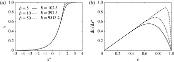
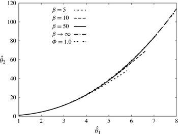
Reference Robin, Mura and Champion2011). The obtained solution, i.e the profile of the progress variable gradient
 $Y(x^{\ast })$
across the flame, the corresponding eigenvalue
 $E$
of the problem, and the progress variable profile
 $c(x^{\ast })$
are provided in figure 1 for different values of the Zel’dovich number
 ${\it\beta}=5$
,
 ${\it\beta}=10$
and
 ${\it\beta}=50$
. The pre-exponential factor and molecular diffusion coefficient values have been set to
 $B=1.2\times 10^{6}~\text{s}^{-1}$
and
 $D_{u}=5\times 10^{-5}~\text{m}^{2}~\text{s}^{-1}$
.
Laminar flame structure
 $c(x^{\ast })$
(a) and its gradient
 $\text{d}c/\text{d}x^{\ast }$
(b) obtained for different values of
 ${\it\beta}$
from numerical simulations considering simplified chemistry and transport properties.

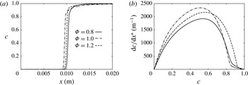
More realistic laminar flame structures are now evaluated from a detailed chemical mechanism using the Cantera library. A methane air flame is considered here for three distinct values of the equivalence ratio
 ${\it\Phi}=0.8$
,
 ${\it\Phi}=1.0$
and
 ${\it\Phi}=1.2$
. Chemistry is described with the detailed GRI3.0 mechanism (Bowman et al.
Reference Bowman, Hanson, Gardiner, Frenklach, Lissianski, Goldenberg, Smith, Crosley and Golden1997). The resulting profiles of the progress variable
 $c(x)$
and the corresponding scalar gradient
 $\text{d}c/\text{d}x$
are presented in figure 2 with the progress variable evolution deduced from
 ${\it\rho}={\it\rho}_{u}/(1+{\it\tau}c)$
. The burning velocities values are respectively
 $28.0~\text{cm}~\text{s}^{-1}$
,
 $38.6~\text{cm}~\text{s}^{-1}$
and
 $33.9~\text{cm}~\text{s}^{-1}$
. The characteristic length scale
 $l_{f}$
of these laminar flame structures are also required to pursue the present analysis. They are evaluated from the maximum value of the scalar gradient, i.e.
 $l_{f}=1/(\text{d}c/\text{d}x)_{max}$
, so that
 $l_{f}=0.52$
mm for
 ${\it\phi}=0.8$
,
 $l_{f}=0.43$
mm for
 ${\it\phi}=1.0$
and
 $l_{f}=0.46$
mm for
 ${\it\phi}=1.2$
. The most striking difference between the results obtained with the simplified chemistry, see figure 1, and the present results obtained with detailed chemistry, which are gathered in figure 2, is associated with the specific behaviour at the burnt gases side. The detailed chemical mechanism leads to a slow evolution of the progress variable from
 $c=0.9$
to
 $c=1.0$
on the burnt gases side. This is clearly visible on the scalar gradient profiles, see figure 2. We will see in the following sections that this specific behaviour has strong consequences not only on the PDF shapes but also on the boundaries of the flamelet structures considered in this study. It is indeed expected that turbulence may alter the laminar flamelet profile in zones where the scalar gradients are rather weak.
Laminar flame structure
 $c(x)$
(a) and its gradient
 $\text{d}c/\text{d}x$
(b) obtained for different values of the equivalence ratio from computations based on a detailed description of chemistry.

According to the discussion of § 2.1, flamelets are presently viewed as laminar flame structure fragments. These flame elements can be determined from the profiles presented in figures 1 and 2 or by considering infinite values of the Zel’dovich number
 ${\it\beta}$
. However, as emphasized in the previous section, their boundaries in the physical space, i.e.
 $x_{max}$
and
 $x_{min}$
, as well as in the composition space, i.e.
 $c_{max}$
and
 $c_{min}$
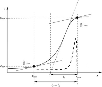
, must – as a prerequisite – be precisely determined from the Karlovitz number value. The following procedure has been retained to this purpose:
-
(1) From the knowledge of the Karlovitz number
 $Ka$
and laminar flame thickness
$l_{f}$
, the flamelet length scale
$l_{x}$
is evaluated from (2.4).
-
(2) Then, the flamelet boundaries in the physical space
$x_{min}$
and
$x_{max}$
are positioned in order to have
$l_{x}=x_{max}-x_{min}$
and
$|\text{d}c/\text{d}x|_{x_{min}}=|\text{d}c/\text{d}x|_{x_{max}}$
.


Description of the procedure retained to define the flamelet boundaries in the physical and composition spaces.

Therefore, following this procedure, which is illustrated in figure 3, the flamelet structure is only composed of the highest values of the scalar gradient. This is consistent with a picture that considers that only the flamelet inner structure is maintained in the turbulent flow, while the smallest scalar gradients associated with the laminar flame structure, i.e.
 $|\text{d}c/\text{d}x|<|\text{d}c/\text{d}x|_{x_{min}}$
(or
 $|\text{d}c/\text{d}x|<|\text{d}c/\text{d}x|_{x_{max}}$
), are altered by the turbulent motions: the leading and trailing edges of the laminar flamelet structure are perturbed by the turbulent flow field (Anand & Pope Reference Anand and Pope1984; Pope & Anand Reference Pope and Anand1984; Mura et al.
Reference Mura, Galzin and Borghi2003). The application of this procedure is restricted to the flamelet regime up to the thin reaction regime, but can no longer be used if the reaction zone is modified by the turbulence. In this case, the whole laminar structure, which is a boundary value problem (BVP), is indeed subject to turbulence modulation by its edges.
In the case of infinitely large values of
 ${\it\beta}$
, the value of
 $c_{max}$
is equal to unity, i.e.
 $c_{max}^{{\it\beta}\rightarrow \infty }=1$
, whatever the value of the flamelet length scale
 $l_{x}$
, i.e. whatever the value of
 $R_{fx}$
. Thus, in this limit, the thickness in the composition space is
 ${\it\delta}_{c}^{{\it\beta}\rightarrow \infty }=1-c_{min}^{{\it\beta}\rightarrow \infty }$
. Therefore, the integration of the preheat zone of the flamelet from
 $c_{min}^{{\it\beta}\rightarrow \infty }$
to
 $c_{max}^{{\it\beta}\rightarrow \infty }=1$
, see (2.3), leads to:
 $$\begin{eqnarray}(\ln (1/c_{min}^{{\it\beta}\rightarrow \infty }))^{-1}=R_{fx}.\end{eqnarray}$$
Moreover, the ratio of the laminar flame thickness
 $l_{f}$
to
 $l_{x}=x_{max}-x_{min}$
, i.e.
 $R_{fx}$
, is related to
 $Ka$
through (2.4). Thus, the minimum value
 $c_{min}^{{\it\beta}\rightarrow \infty }$
is directly related to
 $Ka$
:
 $$\begin{eqnarray}c_{min}^{{\it\beta}\rightarrow \infty }=1-{\it\delta}_{c}^{{\it\beta}\rightarrow \infty }=\exp (-Ka^{-1/2}).\end{eqnarray}$$
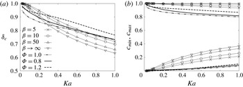
Figure 4 reports the evolution of
 ${\it\delta}_{c}$
,
 $c_{min}$
and
 $c_{max}$
as functions of the Karlovitz number. Whatever the level of description retained (one-step or detailed chemistry), the flamelet thickness in the composition space
 ${\it\delta}_{c}$
is found to decrease with the Karlovitz number value. For finite values of the Zel’dovich number,
 $c_{max}$
is closer to unity than
 $c_{min}$
is close to zero, see figure 4(b). This behaviour is due to the increase of the scalar gradient in the preheat zone, which is weaker than the decrease of the scalar gradient in the reaction zone, see figure 1. An opposite trend is observed when a detailed chemical mechanism is considered because of the specific evolution of the scalar gradient at the burnt gases side of the flame, see figure 2. Figure 4(a) also shows that
 ${\it\delta}_{c}$
decreases with increasing values of the Zel’dovich number because the laminar flame characteristic length scale decreases.
Flamelet thickness
 ${\it\delta}_{c}=c_{max}-c_{min}$
(a), and values
 $c_{min}$
and
 $c_{max}$
(b) as obtained from the different computations based on finite Zel’dovich number or finite-rate, i.e. detailed chemistry, and from the consideration of infinitely large values of the Zel’dovich number.

3. A PDF to represent finite thickness flamelets
3.1. The consequences of flamelet boundaries
The introduction of a specific flamelet length scale leads to a precise definition of their internal structure and boundaries. However, with the objective of describing turbulent flame brushes, the use of these finite thickness flamelets also requires the introduction of a consistent presumed PDF shape. It is chosen here to generalize one of the most studied presumed PDF shapes for turbulent combustion, which is the quasi-bimodal PDF shape introduced in the early analysis of Bray & Moss (Reference Bray and Moss1977). The BML presumed PDF describes the flame brush as composed of three possible states, fresh gases (
 $c\equiv 0$
), fully burnt gases (
 $c\equiv 1$
) and flamelet structures (
 $0<c<1$
). It has been previously demonstrated to be well suited to tackle the flamelet regimes of turbulent premixed combustion that are presently under consideration. Its general form is:
 $$\begin{eqnarray}\widetilde{P}(c,x)={\it\alpha}_{c}{\it\delta}(c)+{\it\beta}_{c}{\it\delta}(1-c)+{\it\gamma}_{c}\widetilde{f}(c),\end{eqnarray}$$
with
 ${\it\alpha}_{c}+{\it\beta}_{c}+{\it\gamma}_{c}=1$
. The function
 $\widetilde{f}(c)$
represents the PDF conditioned in the internal structure of flamelets, i.e
 $0<c<1$
, its normalization condition is:
 $$\begin{eqnarray}\int _{0}^{1}\widetilde{f}(c)\,\text{d}c=1.\end{eqnarray}$$
In the thin flame limit,
 $\widetilde{f}(c)$
can be shown to be inversely proportional to the progress variable gradient through the flame structure
 $\text{d}c/\text{d}x$
. Such a representation holds provided that the flamelet structures remain locally one-dimensional with stretching and curvature effects neglected. Thus, the internal PDF is
 $$\begin{eqnarray}\widetilde{f}(c)=C_{1}^{\ast }(\text{d}c/\text{d}x^{\ast })^{-1},\end{eqnarray}$$
where
 $C_{1}^{\ast }=C_{1}l_{f}$
is a non-dimensionalized normalization constant. Using this PDF shape (3.1), the first- and second-order moments of the progress variable can be written as:
 $$\begin{eqnarray}\displaystyle & \displaystyle \widetilde{c}={\it\beta}_{c}+{\it\gamma}_{c}I_{1}, & \displaystyle\end{eqnarray}$$
 $$\begin{eqnarray}\displaystyle & \displaystyle \widetilde{c^{\prime \prime 2}}={\it\beta}_{c}+{\it\gamma}_{c}I_{2}-\widetilde{c}^{2}, & \displaystyle\end{eqnarray}$$
 $I_{1}$
and
 $I_{2}$
denote the first- and second-order scalar moments conditioned inside the flame structures, which are defined by:
 $$\begin{eqnarray}\displaystyle & \displaystyle I_{1}=C_{1}^{\ast }I_{1}^{\ast },\quad \text{with }I_{1}^{\ast }=\int _{0}^{1}c\frac{\widetilde{f}(c)}{C_{1}^{\ast }}\,\text{d}c=\int _{0}^{1}c(\text{d}c/\text{d}x^{\ast })^{-1}\,\text{d}c=\int _{-\infty }^{+\infty }c(x^{\ast })\,\text{d}x^{\ast }, & \displaystyle\end{eqnarray}$$
 $$\begin{eqnarray}\displaystyle & \displaystyle I_{2}=C_{1}^{\ast }I_{2}^{\ast },\quad \text{with }I_{2}^{\ast }=\int _{0}^{1}c^{2}\frac{\widetilde{f}(c)}{C_{1}^{\ast }}\,\text{d}c=\int _{0}^{1}c^{2}(\text{d}c/\text{d}x^{\ast })^{-1}\,\text{d}c=\int _{-\infty }^{+\infty }c(x^{\ast })^{2}\,\text{d}x^{\ast }, & \displaystyle\end{eqnarray}$$
 $C_{1}^{\ast }$
deduced from (3.2)
 $C_{1}^{\ast }=(\int _{0}^{1}(\text{d}c/\text{d}x^{\ast })^{-1}\,\text{d}c)^{-1}=(\int _{-\infty }^{+\infty }\,\text{d}x^{\ast })^{-1}$
.
However, the practical computation of these integral quantities requires one to set finite values for the integration boundaries, and the constant
 $C_{1}^{\ast }$
is thus evaluated from
 $$\begin{eqnarray}C_{1}^{\ast }=\left(\int _{x_{min}}^{x_{max}}\,\text{d}x^{\ast }\right)^{-1}=(x_{max}^{\ast }-x_{min}^{\ast })^{-1}={\it\delta}_{x^{\ast }}^{-1},\end{eqnarray}$$
and the values retained for the boundaries
 $x_{min}^{\ast }$
and
 $x_{max}^{\ast }$
have strong implications on the integral quantities
 $C_{1}^{\ast }$
,
 $I_{1}$
,
 $I_{2}$
,
 $I_{1}^{\ast }$
,
 $I_{2}^{\ast }$
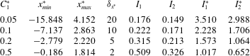
, see table 1 for some examples obtained with
 ${\it\beta}=10$
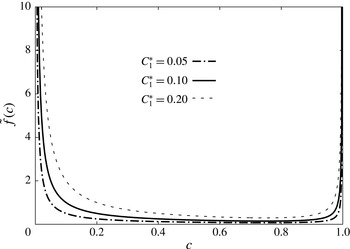
. In figure 5, the PDF
 $\widetilde{f}(c)$
is displayed for different values of the normalization constant
 $C_{1}^{\ast }$
by considering laminar flamelet structures described with simplified chemistry and
 ${\it\beta}=10$
. As expected, the internal PDF
 $\widetilde{f}(c)$
displays a strongly bimodal behaviour with increased probability levels at the boundaries of the domain of definition, i.e.
 $c\rightarrow 0$
and
 $c\rightarrow 1$
. These important levels of probability are associated with the decrease of composition gradients at the boundaries of the flamelet structures. The values retained for the normalization constant
 $C_{1}^{\ast }$
have also strong consequences on the final shapes of the internal PDF, and this highlights the need for a precise definition of the flamelet boundaries, as discussed in the previous sections.
Integral quantities
 $C_{1}^{\ast }$
,
 $I_{1}$
,
 $I_{2}$
,
 $I_{1}^{\ast }$
,
 $I_{2}^{\ast }$
obtained for different values of the integration boundaries
 $x_{min}^{\ast }$
and
 $x_{max}^{\ast }\;({\it\delta}^{\ast }=x_{max}^{\ast }-x_{min}^{\ast })$
and considering single-step global chemistry with
 ${\it\beta}=10$
.

Probability density function of the internal structure of flamelets
 $\widetilde{f}(c)$
obtained from single-step global chemistry with
 ${\it\beta}=10$
for different values of the normalization constant
 $C_{1}^{\ast }$
.

For sufficiently large values of the Damköhler number, the probability
 ${\it\gamma}_{c}$
to lie within flamelet inner structures becomes vanishingly small, i.e.
 ${\it\gamma}_{c}\ll 1$
. It is important to notice that the consideration of this limit implies that the characteristic size of the laminar flame structure is
 $l_{f}$
, which may differ from the thickness
 $l_{x}$
that has been introduced in the previous sections. However, in the limit of infinitely large values of the Damköhler number, the form of the PDF defined by (3.1) reduces to
 $$\begin{eqnarray}\widetilde{P}(c,x)={\it\alpha}_{c}{\it\delta}(c)+{\it\beta}_{c}{\it\delta}(1-c)+\mathit{O}({\it\gamma}_{c}).\end{eqnarray}$$
The progress variable variance
 $\widetilde{c^{\prime \prime 2}}$
reaches its maximum value
 $\widetilde{c}(1-\widetilde{c})$
. This value may be used to normalize the variance levels, thus leading to the segregation rate
 $S$
, which is defined as the ratio of the variance to its maximum possible value, i.e.
 $$\begin{eqnarray}S=\frac{\widetilde{c^{\prime \prime 2}}}{\widetilde{c}(1-\widetilde{c})}.\end{eqnarray}$$
The limit of large Damköhler numbers is then characterized by
 $S\rightarrow 1$
. Eventually, in the limit of large
 $Da$
, the statistical quantities, i.e. variance, turbulent fluxes or higher-order scalar moments are proportional to
 $\widetilde{c}(1-\widetilde{c})$
. This proportionality is the signature of the intermittency between fresh reactants and fully burned gases. Nevertheless, the flamelet PDF (3.1) is not perfectly bimodal and the departure from this bimodal limit, however small it may be, has strong consequences on statistical quantities, especially on the expression of the mean chemical rate. By using (3.4) and (3.5), an expression for the mean chemical rate can be proposed via the probability
 ${\it\gamma}_{c}=(1-S)\widetilde{c}(1-\widetilde{c})/(I_{1}-I_{2})$
, leading to
 $$\begin{eqnarray}\overline{{\it\omega}}={\it\gamma}_{c}I_{{\it\omega}}=(1-S)\widetilde{c}(1-\widetilde{c})I_{{\it\omega}}/(I_{1}-I_{2}),\end{eqnarray}$$
where
 $I_{{\it\omega}}$
is the mean chemical rate conditioned inside the flamelet structures, which can be obtained from laminar flame calculations:
 $$\begin{eqnarray}I_{{\it\omega}}=\int _{0}^{1}{\it\omega}\widetilde{f}(c)\,\text{d}c.\end{eqnarray}$$
Equation (3.11) shows that the mean chemical rate, as other statistical quantities previously discussed, can be written as proportional to
 $\widetilde{c}(1-\widetilde{c})$
. This proportionality to
 $\widetilde{c}(1-\widetilde{c})$
is at the basis of many turbulent combustion closures, see for instance Spalding (Reference Spalding1971, Reference Spalding1976), Bray (Reference Bray, Libby and Williams1980), Mantel & Borghi (Reference Mantel and Borghi1994), Dong et al. (Reference Dong, Robin, Mura and Champion2013). Even if some improvements have been brought to the estimation of the mean chemical rate characteristic time scale, all of these closures still consider a direct proportionality to
 $\widetilde{c}(1-\widetilde{c})$
. However, (3.11) also involves the segregation rate
 $S$
, which is not necessarily constant through the whole flame brush. Therefore, one of the objectives of the present study is to focus on a relevant description of the evolution of the segregation rate
 $S$
through the turbulent flame brush. Such a description may lead to new algebraic closures for the mean chemical rate (cf. (3.11)).
3.2. The segregation rate as a delimiter of the flame brush edges
As just described, considering large values of the Damköhler number leads to
 ${\it\gamma}_{c}\ll {\it\alpha}_{c},{\it\beta}_{c}$
, which allows one to neglect
 ${\it\gamma}_{c}$
in (3.1). However, the leading edge is associated with the appearance of the first flamelet structure in the flow. Thus, at this leading edge the probability to be in fully burnt product may become smaller than the probability to lie inside a flamelet. Therefore, we consider here that the leading edge is characterized by
 ${\it\beta}_{c}\ll {\it\gamma}_{c}$
. Then, the PDF support given by (3.1) reduces to
 $\widetilde{P}(c,x)={\it\alpha}_{c}{\it\delta}(c)+{\it\gamma}_{c}\widetilde{f}(c)$
. The normalization condition of this PDF gives
 ${\it\alpha}_{c}+{\it\gamma}_{c}=1$
, and the first- and second-order moments of the progress variable are written as:
 $\widetilde{c}={\it\gamma}_{c}I_{1}$
, and
 $\widetilde{c^{\prime \prime 2}}={\it\gamma}_{c}I_{2}-\widetilde{c}^{2}$
. Therefore, the segregation rate is:
 $S=(I_{2}/I_{1}-\widetilde{c})/(1-\widetilde{c})$
, a quantity clearly smaller than unity.
For large values of the Damköhler number the probability for a point of the flow to be inside a flamelet is still negligible compared to the probability to be in fresh gases, i.e.
 ${\it\gamma}_{c}\ll {\it\alpha}_{c}$
, so that
 $\widetilde{c}\rightarrow 0$
and the segregation rate at the leading edge is entirely determined from flamelet properties:
 $$\begin{eqnarray}S_{(\widetilde{c}\rightarrow 0)}\rightarrow I_{2}/I_{1}.\end{eqnarray}$$
A similar analysis can be performed at the trailing edge of the flame brush where
 ${\it\alpha}_{c}\ll {\it\gamma}_{c}$
. In this situation, the segregation rate is
 $S=1-(I_{1}-I_{2})/(\widetilde{c}(1-I_{1}))$
. For large values of the Damköhler number, the probability to find a flamelet is negligible in comparison with the fully burnt gases probability, i.e.
 ${\it\gamma}_{c}\ll {\it\beta}_{c}$
so that
 $\widetilde{c}\rightarrow 1$
and the segregation rate at the trailing edge is entirely determined from flamelet properties:
 $$\begin{eqnarray}S_{(\widetilde{c}\rightarrow 1)}\rightarrow 1-(I_{1}-I_{2})/(1-I_{1}).\end{eqnarray}$$
To summarize, when large Damköhler numbers are considered, the segregation rate is close to unity inside the flame brush
 $S\rightarrow 1$
, but does decrease on both edges to reach
 $I_{2}/I_{1}$
at the leading edge and
 $1-(I_{1}-I_{2})/(1-I_{1})$
at the trailing edge. Therefore, (3.13) and (3.14) provide a criterion to delineate the flame brush boundaries, where the bimodal characteristic holds, solely from flamelet properties. In the limit
 ${\it\beta}\rightarrow \infty$
, i.e. when
 $\text{d}c/\text{d}x^{\ast }=c$
, and infinitely thin flamelets, i.e.
 $C_{1}^{\ast }\rightarrow 0$
, the following analytical form of the segregation rate at the leading edge is obtained:
 $$\begin{eqnarray}S_{(\widetilde{c}\rightarrow 0)}=I_{2}/I_{1}=I_{2}^{\ast }/I_{1}^{\ast }=\int _{0}^{1}c\,\text{d}c\left/\int _{0}^{1}\right.\,\text{d}c=1/2.\end{eqnarray}$$
Similarly the following is found at the trailing edge:
 $$\begin{eqnarray}S_{(\widetilde{c}\rightarrow 1)}=1-(I_{1}-I_{2})/(1-I_{1})=1-(I_{1}^{\ast }-I_{2}^{\ast })/((1/C_{1}^{\ast })-I_{1}^{\ast })\rightarrow 1.\end{eqnarray}$$
Eventually, the main conclusion of this analysis is that in the case of high values of the Damköhler and Zel’dovich numbers and considering infinitely thin flamelets (
 $C_{1}^{\ast }=0$
), the segregation rate at the leading edge is not unity but
 $1/2$
. Moreover, the values of the segregation rate at the flame brush edges also depend on the normalization constant
 $C_{1}^{\ast }$
so that the local flame boundaries must be precisely defined via the finite thickness flamelet concept previously introduced.
3.3. Generalized PDF shape
The description of the flamelet characteristic scales introduced in the previous section leads to the introduction of a generalized form of the PDF that takes into account the flamelet finite thickness:
 $$\begin{eqnarray}\widetilde{P}(c,x)={\it\alpha}_{c}{\it\delta}(c-c_{min})+{\it\beta}_{c}{\it\delta}(c_{max}-c)+{\it\gamma}_{c}\widetilde{f}(c),\end{eqnarray}$$
where
 $c_{min}$
and
 $c_{max}$
are the extreme values of the progress variable beyond which the flamelet structures (scalar gradient) are altered by turbulence. It should be emphasized that considering Dirac delta functions at
 $c_{min}$
and
 $c_{max}$
constitutes an important simplification of the PDF support but will allow one to study departures from the infinitely large Damköhler limit associated with
 $c_{min}\rightarrow 0$
and
 $c_{max}\rightarrow 1$
. It is noteworthy that a PDF shape based on two Dirac delta functions has been previously considered in the analysis of Libby & Williams (Reference Libby and Williams2000).
Accordingly the first- and second-order moments of the progress variable are:
 $$\begin{eqnarray}\displaystyle & \displaystyle \widetilde{c}={\it\alpha}_{c}c_{min}+{\it\beta}_{c}c_{max}+{\it\gamma}_{c}I_{1}, & \displaystyle\end{eqnarray}$$
 $$\begin{eqnarray}\displaystyle & \displaystyle \widetilde{c^{\prime \prime 2}}={\it\alpha}_{c}c_{min}^{2}+{\it\beta}_{c}c_{max}^{2}+{\it\gamma}_{c}I_{2}-\widetilde{c}^{2}, & \displaystyle\end{eqnarray}$$
 $$\begin{eqnarray}\displaystyle & \displaystyle I_{1}=\int _{c_{min}}^{c_{max}}c\widetilde{f}(c)\,\text{d}c, & \displaystyle\end{eqnarray}$$
 $$\begin{eqnarray}\displaystyle & \displaystyle I_{2}=\int _{c_{min}}^{c_{max}}c^{2}\widetilde{f}(c)\,\text{d}c, & \displaystyle\end{eqnarray}$$
 $$\begin{eqnarray}\int _{c_{min}}^{c_{max}}\widetilde{f}(c)\,\text{d}c=1.\end{eqnarray}$$
The flamelet properties differ from those associated with the BML limit only through the integration boundaries. The internal PDF still obeys (3.3), but with a normalization constant unambiguously related to the turbulent flamelet characteristic length scale
 $l_{x}$
:
 $C_{1}^{\ast }=(x_{max}^{\ast }-x_{min}^{\ast })^{-1}=l_{f}/(x_{max}-x_{min})=l_{f}/l_{x}\equiv R_{fx}$
, which introduces, via equation (2.4), a dependency of the internal PDF
 $\widetilde{f}(c)$
to the Karlovitz number
 $Ka$
. Therefore the introduction of finite thickness flamelets allows one to define all the parameters that are involved in the PDF support given by (3.17). One can see some similarities between this PDF shape (3.17) and the one introduced in the early analyses by Borghi et al. (Reference Borghi, Argueyrolles, Gauffie and Souhaite1986), Borghi (Reference Borghi1988) which accounts for finite-rate chemistry influence at the leading edge of the flame brush. The main difference between the two approaches lies in the consideration of the flamelet internal PDF
 $\widetilde{f}(c)$
.
The dependence of the above PDF shape on the values of both the Reynolds and Karlovitz numbers now deserves to be analysed further. Considering first the thin flame limit, a quasi-bimodal PDF shape is obtained, i.e.
 ${\it\gamma}_{c}\rightarrow 0$
, and (3.17) becomes:
 $$\begin{eqnarray}\displaystyle \widetilde{P}(c,x)={\it\alpha}_{c}{\it\delta}(c-c_{min})+{\it\beta}_{c}{\it\delta}(c_{max}-c)+\mathit{O}({\it\gamma}_{c}). & & \displaystyle\end{eqnarray}$$
However, the flamelet length scale
 $l_{x}$
is now associated with the smallest length scale of turbulence
 $l_{{\it\eta}_{K}}$
and not to the laminar flame scale
 $l_{f}$
as standardly considered in studies of turbulent combustion regimes. Thus, considering (3.17), the probability to lie inside a flamelet is now related to the Reynolds number. Accordingly, the assumption
 ${\it\gamma}_{c}\rightarrow 0$
in (3.17) is associated with large values of the Reynolds number. This is one of the most important differences between the BML PDF (3.1) and the PDF proposed in (3.17). This specificity is only the consequence of the introduction of the flamelet length scale
 $l_{x}$
, which differs from the laminar flame scale
 $l_{f}$
. Therefore, in the limit of large values of the Reynolds number, the segregation rate reaches its maximum value
 $S_{max}$
, which differs from unity and can be expressed from (3.23):
 $$\begin{eqnarray}\lim _{Re_{t}\rightarrow \infty }S_{max}=\frac{(c_{max}-\widetilde{c})(\widetilde{c}-c_{min})}{\widetilde{c}(1-\widetilde{c})}.\end{eqnarray}$$
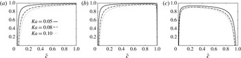
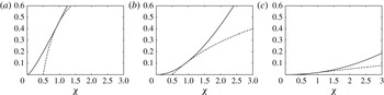
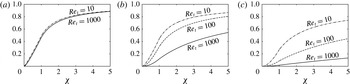
Evolution of the maximum value of the segregation rate
 $S_{max}$
across the flame brush for different values of the Karlovitz number and for the different types of laminar flame structures: infinite values of the Zel’dovich number, i.e. equation (3.25) (a), finite Zel’dovich number but simplified chemistry (b) and detailed description of the chemistry (c).

This expression (3.24) clearly shows that the segregation rate vanishes at both sides of the flame brush when
 $\widetilde{c}\rightarrow c_{min}$
and
 $\widetilde{c}\rightarrow c_{max}$
. The introduction of finite thickness flamelets thus leads to a realistic evolution of the maximum value of the segregation rate through the flame brush without imposing a specific evolution for the mean chemical rate. Moreover, the extreme values
 $c_{min}$
and
 $c_{max}$
that appear in (3.24) are related to the Karlovitz number, as described in previous sections. An analytical expression can be obtained for the segregation rate in the limit of large values of both the Reynolds and Zel’dovich numbers (
 ${\it\beta}\rightarrow \infty$
means
 $c_{max}\rightarrow 1$
): (3.24) leads to
 $S_{max}=1-c_{min}/\widetilde{c}$
, and (2.9) allows one to reveal the Karlovitz number dependence:
 $$\begin{eqnarray}\lim _{Re_{t}\rightarrow \infty ,{\it\beta}\rightarrow \infty }S_{max}=1-\exp (-1/\sqrt{Ka})/\,\widetilde{c}.\end{eqnarray}$$
Figure 6 displays the segregation rate profile for infinite values of the Reynolds number, i.e. (3.24) and for different values of the Karlovitz number. Figure 6(a–c) correspond, respectively, to the case of infinite values of the Zel’dovich number, i.e. (3.25), the case of finite Zel’dovich number but simplified chemistry, and to calculations conducted with detailed chemistry. As expected, these profiles show that the segregation rate varies significantly in small layers on both sides of the flame brush, i.e. the leading and trailing edges. Following the proposed approach, the characteristic thickness of these layers in the composition space is related to the Karlovitz number for the leading edge and both the Karlovitz and Zel’dovich number for the trailing edge. In the limit of infinite values of the Zel’dovich number the layer at the trailing edge disappears completely. In contrast, the consideration of detailed chemistry leads to a thicker layer at the trailing edge. As expected, the layer at the leading edge becomes thicker for increasing values of the Karlovitz number.
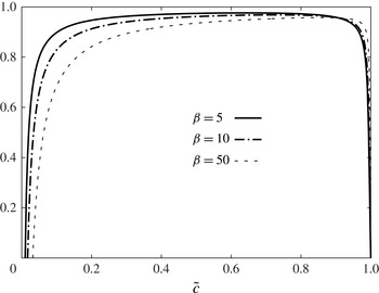
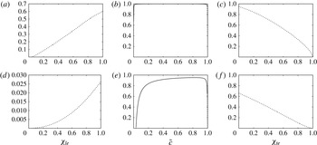
Evolution of the maximum value of the segregation rate
 $S_{max}$
across the flamebrush obtained with single-step chemistry for different values of the Zel’dovich number.

Expression (3.24) and the corresponding figure 7 reproduce qualitatively the evolution that may be postprocessed from DNS databases. It also allows one to estimate the characteristic thickness of both layers at the flame edges, which are related to the Karlovitz and Zel’dovich numbers. It is worth noting that expression (3.24) has been obtained for vanishingly small values of
 ${\it\gamma}_{c}$
, but its knowledge is required to evaluate the mean chemical rate. Thus, the departures from the maximum value of the segregation rate, i.e. denoted here
 $S_{max}$
and given by (3.24) must be considered. The resulting expression for the mean chemical rate is found to be similar to the one obtained in the BML case, as given by (3.11), but the maximum value of the segregation rate is now
 $S_{max}$
instead of unity:
 $$\begin{eqnarray}\overline{{\it\omega}}=(S_{max}-S)\widetilde{c}(1-\widetilde{c})I_{{\it\omega}}/(I_{1}-I_{2}),\end{eqnarray}$$
where
 $I_{{\it\omega}}$
is the mean chemical rate conditioned inside the flamelet structures:
 $$\begin{eqnarray}I_{{\it\omega}}=\int _{c_{min}}^{c_{max}}{\it\omega}\widetilde{f}(c)\,\text{d}c.\end{eqnarray}$$
The modified form of the PDF proposed above uses a generalized description of the segregation rate through the flame brush and gives evidence of the existence of boundary layers associated with the flame edges. Moreover, as demonstrated in § 3.2, the expression for the segregation rate (3.24), which has been obtained for vanishingly small values of
 ${\it\gamma}_{c}$
(
 $Re_{t}\rightarrow \infty$
), no longer holds at the leading edge when the first flamelet appears, i.e.
 ${\it\beta}_{c}\ll {\it\gamma}_{c}$
, and at the trailing edge when the last flamelet disappears, i.e.
 ${\it\alpha}_{c}\ll {\it\gamma}_{c}$
. Accordingly, we now proceed with a refined analysis of the turbulent flame brush.
4. Turbulent flame brush structure
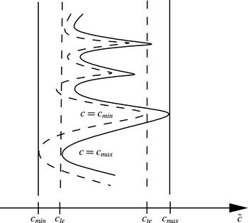
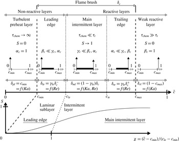
As shown above, the strong decay of the segregation rate that is evidenced on both sides of the flame brush can be related to the Karlovitz number. However, this specific evolution of the segregation rate has been obtained under the assumption of strong bimodality, an assumption that no longer holds at the flame edges. Thus, the turbulent flame brush edges and the turbulent flame brush structure as a whole must now be qualitatively and quantitatively analysed in detail. Figure 8 shows the typical sketch of a turbulent flame brush consistent with the finite thickness flamelet presumed PDF introduced in this paper. Accordingly, the flame brush is delineated by
 $c_{min}<\widetilde{c}<c_{max}$
. Figure 8 illustrates also the appearance of the first flamelet structure and the disappearance of the last flamelet structure, respectively at the leading and trailing edges, associated with the existence of thin layers where the bimodal behaviour no longer holds. The thicknesses of these layers are associated with the laminar flamelet thickness, considered herein to be of the same order of magnitude as the Kolmogorov scale. However, the thicknesses in the composition space of these layers, i.e.
 ${\it\delta}_{le}=c_{le}-c_{min}$
and
 ${\it\delta}_{te}=c_{max}-c_{te}$
, must be evaluated from the knowledge of the Karlovitz number and one additional small parameter, which is the inverse of the turbulent Reynolds number. For large values of the Zel’dovich number we provide below an analytical description of the leading edge, the internal structure of which is studied by using stretched coordinates. Eventually, the description of the reactive flow field is extended beyond these edges, i.e outside the flame brush for
 $\widetilde{c}<c_{min}$
and
 $\widetilde{c}>c_{max}$
.
Structure of the turbulent flame brush.

4.1. Beyond the edges of the flame brush
The flow associated with the smallest values (largest values) of the mean progress variable
 $\widetilde{c}<c_{min}$
, (
 $\widetilde{c}>c_{max}$
), cannot be described within the classical BML framework. However, as emphasized in previous sections, taking into account non-negligible values of the Karlovitz number leads us to consider non-negligible value of
 $c_{min}$
and (
 $1-c_{max}$
). For these very small (or approaching unity) values of the progress variable, the scalar gradient cannot be maintained by chemical reactions so that the turbulent motions are strong enough to promote the mixing of available chemical species. The segregation rate becomes vanishingly small and the progress variable PDF may be approximated from a Dirac delta peak positioned at the mean composition, i.e.
 $\widetilde{P}(c;x)={\it\delta}(c-\widetilde{c})$
.
4.1.1. Turbulent preheat layer
Accordingly, upstream of the turbulent flame brush, a turbulent preheat layer must be considered. The chemical reactions are exponentially small in this zone and can therefore be discarded from its analysis. The physical mechanisms at play lead to an equilibrium between mean convection and turbulent transport:
 $$\begin{eqnarray}{\it\rho}_{u}S_{T}\frac{\text{d}\widetilde{c}}{\text{d}x}=-\frac{\text{d}}{\text{d}x}(\overline{{\it\rho}u^{\prime \prime }c^{\prime \prime }}).\end{eqnarray}$$
Provided that it is modelled with a standard gradient law:
 $\overline{{\it\rho}u^{\prime \prime }c^{\prime \prime }}=-\overline{{\it\rho}}D_{t}\,\text{d}\widetilde{c}/\text{d}x$
, the corresponding turbulent transport mechanism leads to an exponential profile for
 $\widetilde{c}(x)$
in this preheat layer. The physical mechanisms involved in this layer are indeed similar to those involved in the preheat zone of laminar flames, but the transport and propagation mechanisms are controlled by turbulent motions rather than molecular effects. Its thickness in the composition space is
 ${\it\delta}_{pl}=c_{min}$
and so is related to the Karlovitz number.
4.1.2. Weak reactive layer
Downstream of the flame brush for
 $\widetilde{c}>c_{max}$
, the strength of chemical reactions becomes weaker and weaker, i.e. the characteristic chemical time scale becomes large in comparison with the characteristic turbulent time scale. However, contrasting with the turbulent preheat layer (discussed above) where
 $\widetilde{c}=0$
is reached at
 $x\rightarrow -\infty$
, thanks to turbulent transport, chemical reactions here drive the evolution of the mean progress variable towards unity. The characteristic thickness of this layer is
 ${\it\delta}_{rl}=1-c_{max}$
in the composition space. Finally, even though this zone may not be essential to describe the turbulent flame propagation mechanism, it is expected to be important to characterize the formation of polluting species.
4.2. Description of flame brush edges and main intermittent layer
Even though the flame brush is composed of thin flamelets and characterized by a highly intermittent dynamics, the assumption of a vanishingly small value of
 ${\it\gamma}_{c}$
is no longer valid on both edges of the flame brush, corresponding to the first and last flamelet occurrences respectively.
4.2.1. Characteristic thickness of the flame brush edges
In order to evaluate the thickness of these boundary layers, hereafter denoted
 ${\it\delta}_{le}$
and
 ${\it\delta}_{te}$
, the mean progress variable values
 $c_{le}$
and
 $c_{te}$
are introduced and respectively characterized by
 ${\it\beta}_{c}=0$
on the fresh gases side (absence of fully burnt gases) and
 ${\it\alpha}_{c}=0$
on the burnt gases side (absence of fresh reactants), see figure 8. The presumed PDF shape (3.17) allows one to determine the values
 $c_{le}$
and
 $c_{te}$
that are related to (i) the Karlovitz number value, and (ii) the probability to be inside flamelets at these boundaries, i.e.
 ${\it\gamma}_{le}$
and
 ${\it\gamma}_{te}$
. The probability to be inside the flamelet structures at the leading edge
 ${\it\gamma}_{le}$
is associated with the flame brush propagation mechanism. The value retained for
 ${\it\gamma}_{le}$
can be related to the frequency of appearance of these first flamelets. However, the detailed study of the propagation mechanism is beyond the scope of this study. Then, for the sake of simplicity, we consider here that the probability to be inside these smallest structures is proportional to the ratio of their thickness
 $l_{x}=l_{{\it\eta}_{K}}$
to the largest scale of the turbulence, i.e. the integral length scale
 $l_{t}$
, which is responsible for the largest wrinkles of the flame front. Thus the value of
 ${\it\gamma}_{le}$
is approximated by
 ${\it\gamma}_{le}=Re_{t}^{-3/4}$
. For the sake of simplicity, we also consider that the probability to be inside flamelets at the trailing edge is the same as the probability to be inside flamelets at the leading edge, i.e.
 ${\it\gamma}_{le}={\it\gamma}_{te}$
. Then, (3.18) and (3.19), once applied at the leading edge (
 ${\it\beta}_{c}=0$
,
 $\widetilde{c}=c_{le}$
) and trailing edge (
 ${\it\alpha}_{c}=0$
,
 $\widetilde{c}=c_{te}$
) leads respectively to:
 $$\begin{eqnarray}\displaystyle & \displaystyle c_{le}=(1-{\it\gamma}_{le})c_{min}+{\it\gamma}_{le}I_{1}, & \displaystyle\end{eqnarray}$$
 $$\begin{eqnarray}\displaystyle & \displaystyle c_{te}=(1-{\it\gamma}_{te})c_{max}+{\it\gamma}_{te}I_{1}. & \displaystyle\end{eqnarray}$$
Therefore, the thicknesses of the leading and trailing layers, expressed in the mean composition space, are:
 $$\begin{eqnarray}\displaystyle & \displaystyle {\it\delta}_{le}=c_{le}-c_{min}={\it\gamma}_{le}(I_{1}-c_{min}), & \displaystyle\end{eqnarray}$$
 $$\begin{eqnarray}\displaystyle & \displaystyle {\it\delta}_{te}=c_{max}-c_{te}={\it\gamma}_{te}(c_{max}-I_{1}). & \displaystyle\end{eqnarray}$$
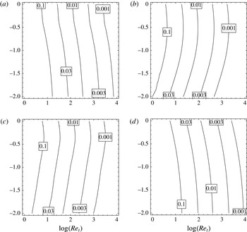
Profiles of the isovalues of
 ${\it\delta}_{le}$
(a,b) and
 ${\it\delta}_{te}$
(c,d) plotted in logarithmic coordinates associated with the Reynolds (abscissa) and Karlovitz number (ordinate). (a,c) Detailed description of chemistry (
 ${\it\phi}=1.0$
). (b,d) Infinite value of the Zel’dovich number.

Then, following the approximation retained above for the inner flamelet probabilities and according to (2.9), the thicknesses of these boundary layers are entirely determined from the knowledge of the Karlovitz and Reynolds numbers. Moreover, (4.4) and (4.5) also show that these thicknesses become vanishingly small for large values of the Reynolds number, since
 ${\it\gamma}_{le}$
and
 ${\it\gamma}_{te}$
tend to zero. However, the effect of the Karlovitz number on these boundary layers will depend on the description retained for the laminar flame structure considered through
 $c_{min}$
,
 $c_{max}$
and
 $I_{1}$
. For example,
 $(I_{1}-c_{min})$
vanishes and
 $(c_{max}-I_{1})$
tends to unity for vanishingly small values of the Karlovitz number when a simplified chemistry is considered.
Considering the limit of infinitely large Zel’dovich number, we obtain analytical expressions for the thicknesses of these boundary layers:
 $$\begin{eqnarray}\displaystyle & \displaystyle {\it\delta}_{le}^{{\it\beta}\rightarrow \infty }=Re_{t}^{-3/4}\left(Ka^{1/2}(1-\exp (-Ka^{-1/2}))-\exp (-Ka^{-1/2})\right), & \displaystyle\end{eqnarray}$$
 $$\begin{eqnarray}\displaystyle & \displaystyle {\it\delta}_{te}^{{\it\beta}\rightarrow \infty }=Re_{t}^{-3/4}(1-Ka^{1/2}(1-\exp (-Ka^{-1/2}))). & \displaystyle\end{eqnarray}$$
 ${\it\delta}_{le}$
in the coordinates (
 $\log Re_{t}$
,
 $\log Ka$
). The isolines are almost vertical. In comparison with the Reynolds number, the weak influence of the Karlovitz number on the thickness of the leading edge layer is clearly shown.
4.2.2. Behaviour of the segregation rate at the edges of the flame brush
Use of the presumed PDF shape (3.17) also leads to the determination of the segregation rates at these boundaries:
 $$\begin{eqnarray}\displaystyle & \displaystyle S_{le}=\frac{(1-{\it\gamma}_{le})c_{min}^{2}+{\it\gamma}_{le}I_{2}-c_{le}^{2}}{c_{le}(1-c_{le})}, & \displaystyle\end{eqnarray}$$
 $$\begin{eqnarray}\displaystyle & \displaystyle S_{te}=\frac{(1-{\it\gamma}_{te})c_{max}^{2}+{\it\gamma}_{le}I_{2}-c_{te}^{2}}{c_{te}(1-c_{te})}. & \displaystyle\end{eqnarray}$$
Therefore, the values of the segregation rate at the boundaries of the bimodal layer are fully determined from the Reynolds and Karlovitz numbers. Once again, in the limit of infinitely large values of the Zel’dovich number
 ${\it\beta}$
, analytical expressions, that are not detailed here, can be derived. Figure 10 displays the isovalues of
 $S_{le}$
in the (
 $\log Re_{t}$
,
 $\log Ka$
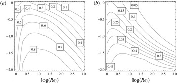
)-coordinates. This figure shows that the maximum value of the segregation rate at the leading edge is obtained for finite values of the Reynolds number. In fact, the effect of the Reynolds number is quite complex since it affects both the value
 $c_{le}$
and the weight of the second-order scalar moment
 $I_{2}$
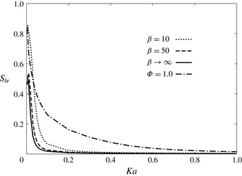
at the leading edge. Figure 10 also confirms that the maximum value of the segregation rate at the leading edge is obtained for vanishingly small values of the Karlovitz number. This maximum value is unity whatever single-step or detailed chemical descriptions are considered, but it is found to be 0.5 in the limit of infinitely large values of the Zel’dovich number. Figure 11 reports the evolution of the segregation rate at the leading edge as a function of the Karlovitz number for large values of the Reynolds number. It is observed that this segregation rate decreases rapidly. The slowest decrease is obtained for a detailed representation of the chemistry, while the highest decrease corresponds to the limit case of infinitely large values of the Zel’dovich number. This behaviour can be compared to that obtained by using the standard BML representation, i.e. bimodal distribution with Dirac delta functions positioned respectively at
 $c=0$
and
 $c=1$
. The asymptotic limit of vanishingly small values of the Karlovitz number are the same for the two PDF shapes, i.e.
 $S_{le}=0.5$
for
 ${\it\beta}\rightarrow \infty$
and
 $S_{te}\rightarrow 1$
for the other cases. However, when the classical BML PDF shape is considered,
 $S_{le}=0.5$
is the minimum possible value of
 $S$
, while the segregation rate at the leading edge can be zero when the PDF shape introduced in this paper is used, see figure 11. Moreover, in the limit of large values of the turbulent Reynolds number but with vanishingly small values of the Karlovitz number, i.e.
 $c_{min}\rightarrow 0$
and
 $c_{max}\rightarrow 1$
, equations (4.8)–(4.9) give
 $S_{le}\rightarrow I_{2}/I_{1}$
and
 $S_{te}\rightarrow 1$
. These expressions are fully consistent with the flame brush boundaries obtained by using the BML PDF shape, as shown in § 3.2. Finally, it is noteworthy that, at the boundary of the leading edge where the assumption of intermittency between reactants at
 $c_{min}$
and products at
 $c_{max}$
may hold, the segregation rate is far from being systematically unity and can even become vanishingly small for non-negligible values of the Karlovitz number.
Profile of the isovalues of
 $S_{le}$
plotted in logarithmic coordinates associated with the Reynolds (abscissa) and Karlovitz number (ordinate): (a) detailed chemistry (
 ${\it\phi}=1.0$
), (b) infinite value of the Zel’dovich number.

Evolution of the segregation rate at the leading edge obtained for
 $Re_{t}=1000$
.

4.2.3. Characteristic thickness of the main intermittent layer
As the flame brush is bounded on each side by two thin layers associated with its leading and trailing edges, the thickness in the composition space of its main (intermittent) layer can be deduced from the thicknesses of the two edge layers just described. Inside the flame brush, at a sufficient distance from these edges, see figure (8), the intermittent nature of the turbulent reactive flows holds: the composition changes abruptly from
 $c=c_{min}$
to
 $c=c_{max}$
. Put in other words, the molecular processes involved in flames occur at the smallest scales of the turbulent flow and the probability
 ${\it\gamma}_{c}$
to lie inside flamelets is small enough to consider that second-order averaged quantities (variance, scalar turbulent fluxes, etc.) are proportional to
 $(c_{max}-\widetilde{c})(\widetilde{c}-c_{min})$
. The thickness
 ${\it\delta}_{ml}$
of the zone where the behaviour of the flame brush can be considered as intermittent is obtained from the characteristic thickness of both boundary layers, see figure (8):
 $$\begin{eqnarray}{\it\delta}_{ml}=c_{te}-c_{le}=(1-{\it\gamma}_{le}){\it\delta}_{c}=(1-{\it\gamma}_{le})(c_{max}-c_{min}).\end{eqnarray}$$
The main layer thickness
 ${\it\delta}_{ml}$
is found to be proportional to the laminar flamelet thickness
 ${\it\delta}_{c}$
and can thus be related to the Karlovitz number. Moreover, it is also dependent on the Reynolds number through the value of
 ${\it\gamma}_{le}$
. For large values of the Reynolds number, the thickness in the mean composition space of the bimodal layer
 ${\it\delta}_{ml}$
tends to the laminar flamelet thickness
 ${\it\delta}_{c}$
. For vanishingly small values of the Karlovitz number, we recover
 ${\it\delta}_{c}=c_{max}-c_{min}=1$
; the thickness in the mean composition space of the bimodal layer
 ${\it\delta}_{ml}$
is only related to the probability to lie inside the flamelet structures at the leading edge
 ${\it\gamma}_{le}$
. Provided that we consider vanishingly small values of the Karlovitz number and large values of the Reynolds number, this main layer thickness tends to unity, i.e.
 ${\it\delta}_{ml}=1$
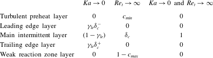
. The limit values associated with each sublayer thickness are gathered in table 2.
Limit values of the characteristic thickness in the composition space of each sublayer of the flame brush. Note that the following definitions are used:
 ${\it\delta}_{c}=c_{max}-c_{min}$
,
 ${\it\delta}_{c}^{-}=I_{1}-c_{min}$
,
 ${\it\delta}_{c}^{+}=c_{max}-I_{1}$
, and
 ${\it\delta}_{c}={\it\delta}_{c}^{+}+{\it\delta}_{c}^{-}$
.

Finally, for sufficiently large Zel’dovich number
 ${\it\beta}$
, and using (2.9), the value of the inner flamelet probability provides an analytical expression for
 ${\it\delta}_{ml}$
that involves only the Reynolds and Karlovitz numbers:
 $$\begin{eqnarray}{\it\delta}_{ml}^{{\it\beta}\rightarrow \infty }=\lim _{{\it\beta}\rightarrow \infty }{\it\delta}_{ml}=(1-Re_{t}^{-3/4})(1-\exp (-Ka^{-1/2})).\end{eqnarray}$$
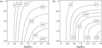
Figure 12 reports isovalues of
 ${\it\delta}_{ml}$
plotted in (
 $\log Re_{t}$
,
 $\log Ka$
) coordinates. The displayed results have been obtained by considering either the limit case of infinitely large values of the Zel’dovich number or a detailed chemical mechanism (
 ${\it\Phi}=1.0$
). The shape of the obtained isolines tends to be vertical on the left bottom part of the figure, i.e. small values of the Reynolds and Karlovitz numbers. This means that the Karlovitz number has only little influence on the characteristic thickness
 ${\it\delta}_{ml}$
. The Reynolds number is the essential parameter for such conditions. This is in sharp contrast with the behaviour observed on the top right side of the figure, which corresponds to large values of the Reynolds and Karlovitz numbers. The isolines obtained here tend to be horizontal. This means that the Reynolds number has only little influence on
 ${\it\delta}_{ml}$
. In such conditions the value of the characteristic thickness is controlled by the Karlovitz number. Similar shapes are obtained for both conditions (large
 ${\it\beta}$
or detailed chemistry) but the obtained thickness
 ${\it\delta}_{ml}$
tends to be thinner when a detailed chemical mechanism is considered.
Profiles of the isovalues of
 ${\it\delta}_{ml}$
plotted in logarithmic coordinates associated with the Reynolds (abscissa) and Karlovitz number (ordinate). (a) Detailed chemistry (
 ${\it\phi}=1.0$
). (b) Infinite value of the Zel’dovich number.

Eventually, this analysis provides a clear bounded domain in the composition space, i.e.
 ${\it\delta}_{ml}$
, where the intermittent behaviour of the flame brush is valid and this domain is fully determined from the values of the Reynolds and Karlovitz numbers. This is expected to be relevant if the purpose is to delineate more precisely the domain where standard turbulent combustion closures, i.e. using a bimodal PDF, apply. To get a deeper understanding of the evolution of averaged quantities from the fresh gases side, where turbulent motions predominate, to this intermittent zone of the flame brush, the internal structure of the leading edge is studied in detail in the following section.
4.3. Connection between the leading and intermittent layers
4.3.1. Internal structure of the leading edge
Within the present description of the turbulent flame brush, the leading edge is considered as the sublayer where the first flamelet appears, see figure 8. The point of view adopted here is similar to the one retained to describe boundary layers in turbulent flows, including the viscous sublayer where molecular processes become dominant, but only within a very thin region in the vicinity of a wall. Accordingly, as wall laws are required to deal with these thin layers in Reynolds-averaged Navier–Stokes (RANS) numerical simulations, we anticipate that a specific treatment will be required to deal with the leading edge in numerical simulations of turbulent flames. The description proposed here constitutes a step in this direction.
The PDF support (3.17) associated with
 ${\it\beta}_{c}=0$
is only valid to determine the boundary
 $c_{le}$
and the consideration of smaller values of the mean progress variable, i.e.
 $c_{min}<\widetilde{c}<c_{le}$
, will require one to account for the smallest scales of turbulence and consider the inner structure of flamelets. At the upstream side of this layer
 $\widetilde{c}\rightarrow c_{min}$
, the structure becomes sensitive to the presence of flamelets with the appearance of the first preheat zone, see figure 8. Thus, at the very beginning of the leading edge, the maximum value found for the progress variable is not
 $c_{max}$
because the trailing edge of the instantaneous flamelet structure does not appear at this location. Accordingly, in this layer, the PDF support (3.17) is modified by replacing
 $c_{max}$
by
 ${\hat{c}}$
, which is an additional parameter of the PDF. The limit situation
 ${\hat{c}}=c_{max}$
is obtained only when the complete structure of the first flamelet appeared. This maximum value of
 ${\hat{c}}$
is reached at the downstream boundary of the leading layer, i.e
 $\widetilde{c}=c_{le}$
. It must be pointed out that, in the limiting case of large values of the Zel’dovich number, this layer is only composed of the preheat zones of flamelets, so that it is a fully non-reactive layer except at the downstream boundary when
 $\widetilde{c}=c_{le}$
, where the reactive sublayer of the leading edge is located. Therefore, in a more general case, this leading layer is reactive only in a small region near its downstream boundary for which its characteristic thickness corresponds to the thickness of the reactive zone of the laminar flamelet.
As the characteristic thickness of this leading layer corresponds to the smallest scale of turbulence and is associated with the characteristic length scale of flamelets, the probability to lie inside flamelet structures is supposed to be constant through the whole leading layer:
 ${\it\gamma}_{c}={\it\gamma}_{le}$
, and the mean and variance of the progress variable can be written as:
 $$\begin{eqnarray}\displaystyle & \displaystyle \widetilde{c}=(1-{\it\gamma}_{le})c_{min}+{\it\gamma}_{le}\hat{I} _{1}, & \displaystyle\end{eqnarray}$$
 $$\begin{eqnarray}\displaystyle & \displaystyle \widetilde{c^{\prime \prime 2}}=(1-{\it\gamma}_{le})c_{min}^{2}+{\it\gamma}_{le}\hat{I} _{2}-\widetilde{c}^{2}, & \displaystyle\end{eqnarray}$$
 $\hat{I} _{1}$
and
 $\hat{I} _{2}$
are similar to equations (3.20) and (3.21) but with
 ${\hat{c}}$
as the upper boundary:
 $$\begin{eqnarray}\displaystyle & \displaystyle \hat{I} _{1}=\int _{c_{min}}^{{\hat{c}}}c\widetilde{f}(c)\,\text{d}c, & \displaystyle\end{eqnarray}$$
 $$\begin{eqnarray}\displaystyle & \displaystyle \hat{I} _{2}=\int _{c_{min}}^{{\hat{c}}}c^{2}\widetilde{f}(c)\,\text{d}c. & \displaystyle\end{eqnarray}$$
 $I_{1}$
and
 $I_{2}$
that correspond to the first and second moments conditioned inside the entire flamelet structures associated with
 ${\hat{c}}=c_{max}$
. Normalization of the partial PDF
 $\widetilde{f}(c)$
yields:
 $$\begin{eqnarray}\int _{c_{min}}^{{\hat{c}}}\widetilde{f}(c)\,\text{d}c=1.\end{eqnarray}$$
Therefore, the mean and variance of the progress variable are both related to the Reynolds number via
 ${\it\gamma}_{le}$
, to the Karlovitz number via
 $c_{min}$
and to the maximum value of the progress variable
 ${\hat{c}}$
. To proceed towards a detailed inspection of the leading edge, stretched coordinates associated with the progress variable
 $c$
, as well as normalized first- and second-order moments conditioned in the flamelets
 $\hat{I} _{1}$
and
 $\hat{I} _{2}$
are introduced:
 $$\begin{eqnarray}{\it\zeta}=\frac{c}{c_{min}},\quad \hat{{\it\theta}}_{1}=\frac{\hat{I} _{1}}{c_{min}},\quad \hat{{\it\theta}}_{2}=\frac{\hat{I} _{2}}{c_{min}^{2}},\end{eqnarray}$$
We also define the normalized upper boundary
 $\hat{{\it\zeta}}={\hat{c}}/c_{min}$
. Substituting the normalized variables defined by (4.17) in (4.14) and (4.15) leads to:
 $$\begin{eqnarray}\displaystyle & \displaystyle \hat{{\it\theta}}_{1}=\int _{1}^{\hat{{\it\zeta}}}{\it\zeta}\widetilde{f}({\it\zeta})\,\text{d}{\it\zeta}, & \displaystyle\end{eqnarray}$$
 $$\begin{eqnarray}\displaystyle & \displaystyle \hat{{\it\theta}}_{2}=\int _{1}^{\hat{{\it\zeta}}}{\it\zeta}^{2}\widetilde{f}({\it\zeta})\,\text{d}{\it\zeta}, & \displaystyle\end{eqnarray}$$
 $\widetilde{f}({\it\zeta})=\widetilde{f}(c)/c_{min}$
. Therefore, from
 $\hat{{\it\theta}}_{1}(\hat{{\it\zeta}})$
and
 $\hat{{\it\theta}}_{2}(\hat{{\it\zeta}})$
, i.e (4.18) and (4.19), the evolution of the second moment conditioned in the flamelets
 $\hat{{\it\theta}}_{2}(\hat{{\it\theta}}_{1})$
can be obtained.
In the limit
 ${\it\beta}\rightarrow \infty$
, (4.18) and (4.19) can be rewritten as:
 $$\begin{eqnarray}\displaystyle & \displaystyle \hat{{\it\theta}}_{1}=C_{1}^{\ast }\int _{1}^{\hat{{\it\zeta}}}\,\text{d}{\it\zeta}=C_{1}^{\ast }(\hat{{\it\zeta}}-1), & \displaystyle\end{eqnarray}$$
 $$\begin{eqnarray}\displaystyle & \displaystyle \hat{{\it\theta}}_{2}=C_{1}^{\ast }\int _{1}^{\hat{{\it\zeta}}}{\it\zeta}\,\text{d}{\it\zeta}=\frac{1}{2}C_{1}^{\ast }(\hat{{\it\zeta}}^{2}-1), & \displaystyle\end{eqnarray}$$
 $$\begin{eqnarray}C_{1}^{\ast }=\left(\int _{1}^{\hat{{\it\zeta}}}{\it\zeta}^{-1}\,\text{d}{\it\zeta}\right)^{-1}=\ln \left(\hat{{\it\zeta}}\right)^{-1}.\end{eqnarray}$$
Then, (4.20) and (4.21) lead to:
 $$\begin{eqnarray}\displaystyle & \displaystyle \hat{{\it\theta}}_{1}=(\hat{{\it\zeta}}-1)\ln (\hat{{\it\zeta}})^{-1}, & \displaystyle\end{eqnarray}$$
 $$\begin{eqnarray}\displaystyle & \displaystyle \hat{{\it\theta}}_{2}={\textstyle \frac{1}{2}}(\hat{{\it\zeta}}^{2}-1)\ln (\hat{{\it\zeta}})^{-1}, & \displaystyle\end{eqnarray}$$
 $$\begin{eqnarray}-\frac{\exp (-1/\hat{{\it\theta}}_{1})}{\hat{{\it\theta}}_{1}}=-\frac{\hat{{\it\zeta}}}{\hat{{\it\theta}}_{1}}\exp \left(-\frac{\hat{{\it\zeta}}}{\hat{{\it\theta}}_{1}}\right)\end{eqnarray}$$
which is solved as
 $\hat{{\it\zeta}}=f(\hat{{\it\theta}}_{1})$
using the secondary real branch
 $W_{-1}$
of the Lambert function (Corless et al.
Reference Corless, Gonnet, Hare, Jeffrey and Knuth1996):
 $$\begin{eqnarray}\hat{{\it\zeta}}=-\hat{{\it\theta}}_{1}W_{-1}\left(-\frac{\exp (-1/\hat{{\it\theta}}_{1})}{\hat{{\it\theta}}_{1}}\right).\end{eqnarray}$$
Now, using (4.26), the second-order moment conditioned in the flamelets, given by (4.24), can be obtained as a function of the first-order moment:
 $$\begin{eqnarray}\hat{{\it\theta}}_{2}=\frac{\left(\hat{{\it\theta}}_{1}W_{-1}\left(-{\displaystyle \frac{\exp (-1/\hat{{\it\theta}}_{1})}{\hat{{\it\theta}}_{1}}}\right)\right)^{2}-1}{2\ln \left(-\hat{{\it\theta}}_{1}W_{-1}\left(-{\displaystyle \frac{\exp (-1/\hat{{\it\theta}}_{1})}{\hat{{\it\theta}}_{1}}}\right)\right)}.\end{eqnarray}$$
Evolution of the second-order moment conditioned in the flamelets
 $\hat{{\it\theta}}_{2}$
as a function of the first-order moment conditioned in the flamelets
 $\hat{{\it\theta}}_{1}$
considering either the limit of infinitely large values of the Zel’dovich number, i.e. equation (4.27), single-step or detailed chemistry.

Figure 13 shows the evolution of the second-order moment conditioned in the flamelets
 $\hat{{\it\theta}}_{2}$
inside the leading edge for the different flames considered in this study, including the limit case of infinite values of the Zel’dovich number as given by (4.27). Thanks to the definition used for
 $\hat{{\it\theta}}_{1}$
and
 $\hat{{\it\theta}}_{2}$
, the Karlovitz and Reynolds numbers do not affect the shapes of the curves presented in figure 13. Only the internal structure of laminar flames, as described with simplified or detailed chemical mechanisms, can influence these second-order moment evolutions, though the value of the Karlovitz number changes the extrema of these first- and second-order moments conditioned in the flamelets. Therefore, the stretched coordinates
 $\hat{{\it\theta}}_{1}$
and
 $\hat{{\it\theta}}_{2}$
are now both normalized as:
 $$\begin{eqnarray}{\it\chi}=\frac{\hat{{\it\theta}}_{1}-1}{{\it\theta}_{1}-1},\quad {\it\psi}=\frac{\hat{{\it\theta}}_{2}-1}{{\it\theta}_{2}-1},\end{eqnarray}$$
where
 ${\it\theta}_{1}$
and
 ${\it\theta}_{2}$
are respectively
 $I_{1}/c_{min}$
and
 $I_{2}/c_{min}^{2}$
, functions of the Karlovitz number. These normalized variables are related to
 $\widetilde{c}$
and
 $\widetilde{c^{2}}$
as follows:
 $$\begin{eqnarray}{\it\chi}=\frac{\widetilde{c}-c_{min}}{c_{le}-c_{min}},\quad {\it\psi}=\frac{\widetilde{c^{2}}-c_{min}^{2}}{(\widetilde{c^{2}})_{le}-c_{min}^{2}}.\end{eqnarray}$$
Then, from (4.28), the evolution of
 ${\it\psi}({\it\chi})$
through the leading layer is:
 $$\begin{eqnarray}{\it\psi}=\frac{1}{{\it\theta}_{2}-1}\left({\displaystyle \frac{\left((1+{\it\chi}({\it\theta}_{1}-1))W_{-1}\left(-\displaystyle \frac{\exp (-1/(1+{\it\chi}({\it\theta}_{1}-1)))}{(1+{\it\chi}({\it\theta}_{1}-1))}\right)\right)^{2}-1}{2\ln \left(-(1+{\it\chi}({\it\theta}_{1}-1))W_{-1}\left(-{\displaystyle \frac{\exp (-1/(1+{\it\chi}({\it\theta}_{1}-1)))}{(1+{\it\chi}({\it\theta}_{1}-1))}}\right)\right)}}-1\right).\end{eqnarray}$$
In the case of infinitely thin flames, i.e.
 $Ka\rightarrow 0$
, the above (4.30) reduces to
 ${\it\psi}={\it\chi}^{2}$
. Eventually, from the second-order moment
 ${\it\psi}({\it\chi})$
, the evolution of the segregation rate
 $S({\it\chi})$
through the leading edge, i.e.
 ${\it\chi}<1$
, can be obtained and compared to the evolution of the segregation rate
 $S({\it\chi})$
through the intermittent layer, i.e.
 ${\it\chi}>1$
, see figure 14.
Segregation rate profile as obtained for infinitely large values of the Zel’dovich number,
 $Re_{t}=1000$
and distinct values of the Karlovitz number (
 $Ka=0.01$
(a), 0.03 (b), 0.1 (c)). The continuous lines correspond to the solution of the leading edge internal structure valid for
 ${\it\chi}<1$
, while the dashed lines correspond to the intermittent layer solution valid for
 ${\it\chi}>1$
.

4.3.2. Internal structure of the intermittent layer
For finite values of the Reynolds number, the profile of the segregation rate within the main intermittent layer can be deduced from the first- and second-order centred moments of the progress variable, through equations (3.18) and (3.19). As emphasized above the knowledge of
 ${\it\gamma}_{c}$
is required to determine the segregation rate through the whole flame brush. However, close to the leading edge, it is considered that
 ${\it\gamma}_{c}$
is almost constant, i.e.
 ${\it\gamma}_{c}={\it\gamma}_{le}$
, and may thus be related to the Reynolds number. This assumption, once applied to (3.18) and (3.19), allows one to express the segregation rate as a function of
 $Re_{t}$
,
 $Ka$
and the mean progress variable. Moreover, it ensures a perfect continuity between the solutions obtained in the internal structure of the leading edge and in the main intermittent layer, since the two segregation rate solutions match at
 ${\it\chi}=1$
. Figure 14 displays the evolution of the segregation rate from the beginning of the leading edge at
 ${\it\chi}=0$
to the main intermittent layer (
 ${\it\chi}\rightarrow \infty$
) for different values of
 $Ka$
. As expected, it increases slowly for the largest values of the Karlovitz number. It is also observed that the solution of the internal structure of the leading edge is strongly curved for large values of the Karlovitz number, while it is almost a straight line for vanishingly small values of this number. This behaviour is a direct outcome of the properties of the Lambert functions involved in the solution of the internal structure of the leading edge.
Complete solution of the segregation rate evolution at the leading edge for infinitely large values of the Zel’dovich number and different values of the Reynolds and Karlovitz number (
 $Ka=0.01$
(a), 0.03 (b), 0.1 (c)).

Profiles of the segregation rate across the entire flame brush structure obtained for
 $Re_{t}=1000$
and
 $Ka=0.01$
(a–c) and
 $Ka=0.1$
(d–f), with
 ${\it\chi}_{le}={\it\chi}=(\tilde{c}-c_{min})/(c_{le}-c_{min})$
and
 ${\it\chi}_{te}=(\tilde{c}-c_{te})/(c_{max}-c_{te})$
. The value of the Zel’dovich number is set to
 ${\it\beta}=10$
.

The complete solutions that have been derived from the present analysis are plotted in figure 15 for various values of the Reynolds number. The first remarkable result is that the increase of the segregation rate is smaller for the largest values of the Reynolds number. This behaviour is explained by the thickness of the leading edge, which is thinner for larger values of the Reynolds number, i.e.
 ${\it\delta}_{le}\rightarrow 0$
for
 $Re_{t}\rightarrow \infty$
, see equation (4.6), so that the bimodal limit is reached for larger values of
 ${\it\chi}$
. The second important result is that for vanishingly small values of the Karlovitz number, the profiles of the segregation rate tend to be the same whatever the values of the Reynolds number. Actually, for
 $Ka\rightarrow 0$
, i.e. infinitely thin flamelets, and
 ${\it\beta}\rightarrow \infty$
, the asymptotic segregation rate profile
 $S({\it\chi})$
obtained in the intermittent layer is given by:
 $$\begin{eqnarray}S=1-(2\,{\it\chi})^{-1},\quad \text{for }{\it\chi}>1,\text{ with }{\it\beta}\rightarrow \infty \text{and }Ka\rightarrow 0,\end{eqnarray}$$
and in the leading edge layer:
 $$\begin{eqnarray}S={\it\chi}/2,\quad \text{for }{\it\chi}<1,\text{ with }{\it\beta}\rightarrow \infty \text{and }Ka\rightarrow 0,\end{eqnarray}$$
The procedure retained above to describe the leading edge can also be applied to flames described with either global or detailed chemistry. However, the description of the chemistry prevents the obtention of analytical expressions. For instance, figure 16 provides the profiles of the segregation rate across the entire flame brush structure as obtained from the consideration of single-step chemistry with
 ${\it\beta}=10$
. As already evidenced with
 ${\it\beta}\rightarrow \infty$
, the segregation rate profile at the leading edge tends to be a straight line for vanishingly small values of the Karlovitz number. It is also worth noting that the segregation profile displayed in figure 16 is consistent with those postprocessed from DNS databases, see for instance Mura et al. (Reference Mura, Tsuboi and Hasegawa2008). The results obtained in this section are gathered in figure 17, which displays the different non-reactive and reactive sublayers that compose the turbulent flame brush, with emphasis on the transition between the leading edge sublayer and the main intermittent layer. The Reynolds number controls the thickness of the leading edge layer, while the Karlovitz number controls its internal structure and so the evolution of the second-order moment towards a bimodal behaviour.
Summary of the main results, including each sublayer of the turbulent premixed flame brush with its characteristic thickness and associated dependences on the turbulent Reynolds number and Karlovitz number.

Before concluding, it must be emphasized that the analysis of both the leading and trailing edges still requires additional work. As an example, the influence of dilatation as well as the viscosity increase at the trailing edge may indeed deserve further attention. Concerning the latter effect, viscosity changes may be partly taken into account by considering the corresponding local variations of the Karlovitz and Reynolds numbers. The molecular viscosity of the mixture could be deduced from the composition statistics. The Karlovitz and Reynolds numbers are evaluated as functions of the local mixture and flow characteristics. Critically strained or critically curved flamelets may also play a crucial role in the flame dynamics, as emphasized in the leading points model of turbulent flame propagation introduced by Zel’dovich & Frank-Kamenetskii (Reference Zel’dovich and Frank-Kamenetskii1947), see also Amato & Lieuwen (Reference Amato and Lieuwen2014). Fast propagating, highly perturbed, i.e. curved and strained, reacting structures indeed concentrate on the leading edge and are thus expected to control to a large extent the propagation of the turbulent flame brush. These highly curved and strained leading edges can undergo local extinctions. Incorporating such flame strain and curvature effects is difficult in a theoretical analysis but could be attempted in forthcoming developments of turbulent combustion closures based for instance on a tabulation methodology. However, it is acknowledged that the proper choice of edge flame building blocks as strained planar flames, expanding (or converging) spherical flames, and expanding cylindrical flames, is prone to debate (Lipatnikov Reference Lipatnikov2013).
5. Conclusions
For premixed conditions, classical combustion diagrams do provide a useful picture of the interaction between combustion and turbulence. However, they do not give a detailed view of the structure of the turbulent premixed brush. Therefore the subject of the present study is the description and analysis of this brush. In this work, after a brief introduction of the physical mechanisms and associated characteristic length and time scales, the structures of laminar premixed flames are considered as flamelet building blocks. Then, the standard BML approach is considered and subsequently modified to deal with the description of the boundaries of turbulent flame brushes where the influence of laminar flame finite thickness becomes non-negligible. Finally, a layered description of the turbulent premixed flame brush is proposed. The obtained results complete usefully classical turbulent combustion diagrams. In particular, a refined description of turbulent premixed flame brushes that reflects the influence of both the Reynolds and the Karlovitz number is obtained. This allows one to get further insights into the layered structure of the premixed turbulent flame brush in terms of boundary layers using the Karlovitz number as the suitable small characteristic parameter. The evolution of the progress variable segregation rate as a relevant marker of turbulence–chemistry interactions is central to this discussion. Special attention is also paid to the leading edge, the influence of which is known to be essential to determine flame brush propagation features. An analytic description of this leading edge is indeed obtained in the limit case of infinitely large values of the Zel’dovich number, showing that, once properly normalized, the second-order moment follows the secondary real branch
 $W_{-1}$
of a Lambert function. The behaviour of the leading edges is also analysed for situations featuring finite values of the Zel’dovich number as well as finite-rate chemistry effects through the consideration of detailed chemical schemes. Finally, another interesting point concerns turbulent combustion modelling. Turbulent combustion closures do often involve the closure of a transport equation for a progress variable variance or segregation rate, which requires a specific closure for the scalar dissipation rate to be settled. The most recent analyses have confirmed that this quantity remains very difficult to represent, and the corresponding closures rely on quite complex expressions that involve many modelling parameters and constants. Since it leads to an analytical description of the segregation rate evolution through the flame brush, the above investigation may provide an interesting way to circumvent the difficulties associated with the use of such complicated closures.