II. SS RELATIONSHIP

Material properties are obtained from load–displacement curves from tensile tests. First, the point where the load decreases for the first time (necking point) is to be determined. Up to the necking point, true stress σ_t and true strain ε_t can be calculated by

(1) $${{\rm{\sigma }}_{\rm{t}}} = {{\rm{\sigma }}_{\rm{e}}}(1 + {{\rm{\varepsilon }}_{\rm{e}}})\,;\,{{\rm{\varepsilon }}_{\rm{t}}} = \ln (1 + {{\rm{\varepsilon }}_{\rm{e}}})\quad .$$

After necking, mean true SS values can be obtained by

(2) $${{\rm{\sigma }}_{\rm{t}}} = P{\rm{/}}A\,;\,{{\rm{\varepsilon }}_{\rm{t}}} = \ln \,({A_{\rm{0}}}{\rm{/}}A)\quad ,$$

where A, A ₀, and P are current cross-sectional area, initial cross-sectional area, and tensile load, respectively; σ_e and ε_e are engineering stress and engineering strain, respectively. Prior to necking, the specimen is in a uniaxial stress state, whereas after necking, it is in a triaxial stress state. Since the flow stress associated with a triaxial stress state is bigger than the flow stress associated with a uniaxial stress state, an appropriate correction is required. Bridgman ^{Reference Bridgman9} suggested the following equations to calculate the stresses in the smallest cross-section

(3) $${{\rm{\sigma }}_{\rm{r}}} = {{\rm{\sigma }}_{\rm{t}}} = {{{{\rm{\sigma }}_{{\rm{am}}}}} \over {\left( {1 + 2R/a} \right)}}\left[ {{{\ln \left( {{{{a^2} \,+ \,2aR \,- \,{r^2}} \over {2aR}}} \right)} \over {\ln \left( {1 + {a \over {2R}}} \right)}}} \right]\quad ,$$

(4) $${{\rm{\sigma }}_{\rm{a}}} = {{{{\rm{\sigma }}_{{\rm{am}}}}} \over {\left( {1 + 2R/a} \right)}}{{1 + \ln \left( {{{{a^2}\, + \,2aR \,- \,{r^2}} \over {2aR}}} \right)} \over {\ln \left( {1 + {a \over {2R}}} \right)}}\quad ,$$

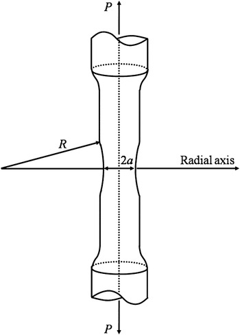
where σ_r, σ_t, σ_a, and σ_am are radial, hoop, axial, and mean axial stress, respectively. R is the radius of curvature in the necking region, a is the radius of the smallest cross-section, and r is the radial distance from the centerline (Fig. 1). Neglecting shear stresses, the equivalent stress can be calculated by

(5) $${{\rm{\sigma }}_{\rm{e}}} = {1 \over {\sqrt 2 }}{\left[ {{{({{\rm{\sigma }}_{\rm{r}}} - {{\rm{\sigma }}_{\rm{t}}})}^2} + {{({{\rm{\sigma }}_{\rm{t}}} - {{\rm{\sigma }}_{\rm{a}}})}^2} + {{({{\rm{\sigma }}_{\rm{a}}} - {{\rm{\sigma }}_{\rm{r}}})}^2}} \right]^{1/2}}\quad ,$$

so that the ratio of equivalent stress to mean axial stress is

(6) $${{{{\rm{\sigma }}_{\rm{e}}}} \over {{{({{\rm{\sigma }}_{\rm{a}}})}_{{\rm{mean}}}}}} = {1 \over {\left( {1 + {{2R} \over a}} \right)\left[ {\ln \left( {1 + {a \over {2R}}} \right)} \right]}} = B\quad ,$$

where B is the Bridgman correction factor. Generally, the value of B has to be less than 1 after diffuse necking. A drawback of Bridgman's correction method is that R and a have to be measured (which is difficult).

FIG. 1.

Schematic of necking in tensile specimen.

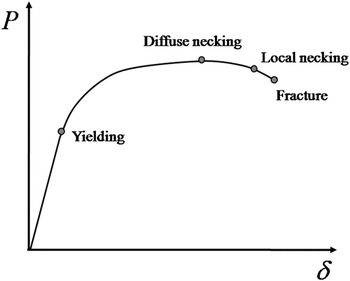
Sheet specimens show characteristics different from those of round specimen. Figure 2 shows a typical load–displacement curve for ductile metal sheet specimens. The elastic–plastic deformation is uniform up to the onset of diffuse necking, but nonuniform afterwards. Once diffuse necking has set in plate specimens, the cross-section loses its initially rectangular shape and fracture generally happens only shortly afterward. Therefore, to obtain mean true SS curves, the current area A has to be measured in the minimum cross-section. Zhang et al. ^{Reference Zhang, Hauge, Odegard and Thaulow16} expressed the reduction of cross-sectional area as a function of thickness reduction.

FIG. 2.

Schematic plot of the load–displacement record from a tension test.

Scheider et al. ^{Reference Scheider, Brocks and Cornec17} proposed a correction factor for rectangular specimens by means of which a triaxial stress state can be converted into a uniaxial stress state (effective stress). Unlike the Bridgman coefficient, this correction method takes into account the change in cross-section. However, the method suggested by Zhang et al. ^{Reference Zhang, Hauge, Odegard and Thaulow16} is only applicable to isotropic materials and when the thickness reduction relative to the initial thickness is below 50%.

III. TENSILE TEST AND FINITE ELEMENT MODELING

Tensile tests are performed with plate specimens of four different materials: Al6061, SS400, Zircaloy-4, and Zirlo. The load–displacement curve of Al6061 can be approximated by a power law, whereas that of SS400 can only be described by a function that is somewhere between a power law and a linear function. The mechanical behavior of Zircaloy-4 and Zirlo can be expressed by bilinear functions. Note that cracking or tearing may occur during stamping of Zircaloy-4 and Zirlo sheets. ^{Reference Hyun, Kim, Lee and Kim18,Reference Hyun, Kim, Lee and Kim19} An accurate evaluation of material properties for Zircaloy-4 and Zirlo is therefore important.

Tensile specimens are made according to Korea Standard 13B, that is, width W = 12.5 mm, gauge length L _g = 50 mm, parallel body length L _p = 60 mm, radius of shoulder r = 25 mm, and thickness t = 0.5 mm for Zircaloy-4 and Zirlo, 4.0 mm for Al6061 and 3.7 mm for SS400. Since the effect of load application rate is negligible in normal tensile tests, load is applied with a rate of 5.0 mm/min. Anisotropy coefficient tests are performed with Zircaloy-4 and Zirlo specimens. Samples are prepared featuring three different angles α between rolling and loading directions (α = 0°, 45,° and 90°). For tensile tests, only specimens with α = 0° are used. Anisotropy coefficient tests are performed with specimens featuring a grid of 2 × 2 mm² squares imprinted on the specimen surface. The strain in thickness direction can be calculated by means of the condition of plastic incompressibility

(7) $${{\rm{\varepsilon }}_{\rm{1}}} + {{\rm{\varepsilon }}_2} + {{\rm{\varepsilon }}_3} = 0\quad ,$$

where ε₁, ε₂, and ε₃ are the strains in length, width, and thickness directions. The anisotropy coefficient r is defined as

(8) $$r \;\equiv\; {{\rm{\varepsilon }}_2}/{{\rm{\varepsilon }}_3}\quad .$$

The anisotropy coefficient is calculated from the grid deformation before necking (elongation = 15%). In this study, the normal anisotropy coefficient r _n is obtained from the anisotropy coefficients according to three different angles α (= 0°, 45°, and 90°) between rolling and loading directions.

(9) $${r_{\rm{n}}} = {{{r_{\rm{0}}} + 2{r_{{\rm{45}}}} + {r_{{\rm{90}}}}} \over 4}\quad .$$

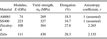
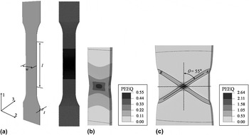
In this paper, we consider the r _n obtained by Eq. (9) as the anisotropy coefficient r. Mechanical properties and anisotropy coefficients are listed in Table I. For FE analysis, the commercial program ABAQUS ²⁰ is used. Figure 3(a) shows the FE models for plate specimens. Considering only loading and geometric symmetry, an FE model comprising one fourth or one eighth of the tensile specimen could be adopted. However, the deformation depends on the material properties and the geometry of the specimen. The angle θ between neck and loading axis, for instance, varies with the aspect ratio W/t and the strain-hardening exponent n [Fig. 3(b)]. ^{Reference Hyun, Kim, Lee and Kim18} Since in real tensile tests generally asymmetric deformation occurs and a single localized band [such as A or B in Fig. 3(c)] develops, a full FE model needs to be used. The FE model consists of about 180,000 8-node brick elements (C3D8) and 130000 nodes (ABAQUS, 2010). ²⁰

TABLE I.

Mechanical properties and anisotropy coefficient for four different specimens.

FIG. 3.

(a) FE models for plate tensile test specimens, and the distribution of equivalent plastic strain with aspect ratio (W/t) and n; (b) W/t = 5, n = 0.1; and (c) W/t = 15, n = 0.05.

Ductile rupture in metals is usually accompanied by necking phenomena, rendering applicable the Gurson–Tvergaard–Needleman (GTN) model. ^{Reference Gurson21,Reference Tvergaard and Needleman22} However, the GTN model requires additional material parameters that are difficult to obtain and is therefore not applied here. Instead, we perform geometrically nonlinear FE analyses assuming isotropic or anisotropic elastic–plastic materials that obey the Mises or the Hill yield criteria.

When analyzing tensile tests with plate specimens, the necking phenomena can be simulated by incorporating flaws in the initial FE model or by adding head and shoulder of the specimen. Assuming large initial flaws, stresses are overestimated in FEA and the resulting SS curve is influenced by the size and shape of the induced flaws.

Zhang et al. ^{Reference Zhang, Ødegard, Sovik and Thaulow23} investigated the influence of initial flaws oriented in the plate specimen's thickness direction on the material's real SS curve. If the specimen's shoulder radius is three times the specimen thickness, the stress error (the deviation of the experimental stress value from the stress obtained by FE analysis) hardly exceeds the relative size of the flaw (relative to the specimen width) in the specimen's width direction. The stress error can be controlled via the size of the initial notch radius. ^{Reference Zhang, Ødegard, Sovik and Thaulow23} However, if head and shoulder are added to the FE model, the necking phenomenon can be simulated without introducing initial flaws. In this study, the latter method is applied; head and shoulder are identical to those of actual test specimens.

IV. PREDICTION OF LOCAL NECKING

A. Theoretical prediction of local necking

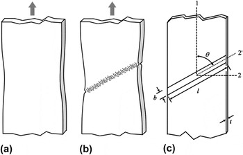
We speak of necking when heterogeneous deformations occur in a tensile test specimen. Diffuse necking has set in when these heterogeneous deformations range over a length greater than the specimen thickness and occur at maximum tensile load [Fig. 4(a)]. The strain value at diffuse necking is equal to the strain hardening coefficient n for isotropic materials. In plate specimens, local necking (i.e., highly unstable deformation) generally occurs between diffuse necking and fracture [Fig. 4(b)]. When local necking occurs, material on both sides of the neck is not (further) deformed. Although contraction in width direction is prevented, local necking is accompanied by strain reduction in both width and thickness directions [Fig. 4(c)]. Under uniaxial loading conditions, the critical strain at which local necking sets in is ε₁ = 2n. ^{Reference Hill24} For biaxial stretching, the following equation must be satisfied

(10) $${{\rm{\varepsilon }}_1} = {n \over {1 + {\rm{\rho }}}}\quad ,$$

where ρ is the strain ratio ε₂/ε₁. For anisotropic material subject to uniaxial tension, ρ can be expressed in terms of the normal anisotropy coefficient r.

(11) $${\rm{\rho }} = {{\rm{\varepsilon }}_2}{\rm{/}}{{\rm{\varepsilon }}_1} = - {r \over {1 + r}}\quad .$$

FIG. 4.

Development of a diffuse neck (a), localized neck (b), and coordinate axes used in the analysis are shown in (c).

Combining Eqs. (10) and (11), we get for the local necking strain ε₁ = n (1 + r).

B. Analytical prediction of local necking

Since the width of local necking is approximately equal to the thickness, the elongation after local necking is generally very small and failure occurs very soon (Fig. 2). FE analysis data are valid only up to local necking so that the onset of local necking may be considered as the validity limit of true SS data. To predict local necking, we use the ratio of strain sets.

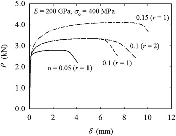
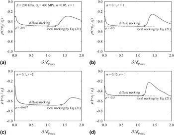
We obtain load–displacement (P–δ) curves for isotropic materials with elastic modulus E = 200 GPa, yield strength σ₀ = 400 MPa, and different strain-hardening exponents n = (0.05, 0.1, 0.15) and for one anisotropic material with n = 0.1 and r = 2 (Fig. 5). Since strains are maximum in the center of the plate specimen, local necking and fracture occur there. We observe the change of minor/major strains at the center of specimen. The ratio ρ has a constant value of −0.5 (r = 1) and −0.67 (r = 2) up to the onset of local necking; once strains start to concentrate in the local necking region, |ρ| decreases rapidly (Fig. 6). The hardening in the neck counteracts the width reduction, while the stress components there remain at constant ratios. The more pronounced the strain hardening, the larger is the deformation. We express the onset of local necking in terms of $\left| {{{\rm{\rho }}_{P{\rm{max}}}}} \right|$ (ρ-value at maximum load) and n (Fig. 6)

(12) $$\left| {{{\rm{\rho }}_{{\rm{local}}}}} \right| = \left| {{{\rm{\rho }}_{{P_{\max }}}}} \right|\left( {1 - cn} \right)\quad .$$

FIG. 5.

Load–displacement curves for various values of n.

FIG. 6.

The ratio of ε₂ to ε₁ versus displacement for various values of n.

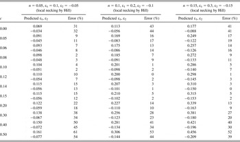
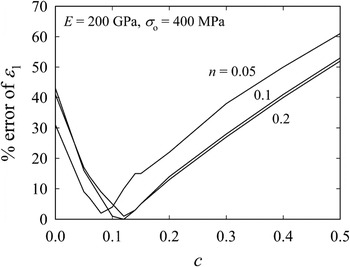
To determine the range of c that yields an error between theoretical local strains and those predicted by Eq. (12) of less than 5%, we start off by assuming a value for c ∈ [0, 0.5] and calculate |ρ_local| for n = (0.05, 0.1, 0.15). FEA values for ε₁ and ε₂ corresponding to |ρ_local| are then compared to theoretical local strains. Doing so, we obtain c ∈ [0.08, 0.1] for n = 0.05, c ∈ [0.1, 0.15] for n = 0.1, and c ∈ [0.1, 0.15] for n = 0.15 (Table II and Fig. 7). The common value of c (c = 0.1) is finally taken to predict local necking for the range n = ∈ [0, 0.5, 0.15]. If the power law SS relation is used, i.e., σ = Kε ⁿ , n is equal to ε₁|P _max. Equation (12) can then be written as

(13) $$\left| {{\rm{\rho }}_{{\rm{local}}} } \right| = \left| {{\rm{\rho }}_{P_{\max } } } \right|\left( {1 - 0.1\left. {{\rm{\varepsilon }}_1 } \right|_{P_{\max } } } \right)\quad .$$

TABLE II.

Error of predicted minor/major strain for three different n.

FIG. 7.

Error of predicted major strain ε₁ with coefficient c for three different n.

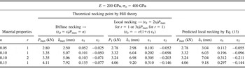
In Table III, strains (ε₁, ε₂) calculated by Eq. (14) are compared with the strains from Hill's theory. To evaluate the point of local necking, we determine by FEA the absolute value of the principal strain at the specimen's center and the principal strain ratio at maximum tensile load (ε₁|P _max and $\left| {{{\rm{\rho }}_{{P_{{\rm{max}}}}}}} \right|$ ). Inserting in Eq. (13) then delivers the principal strain ratio at local necking.

TABLE III.

Obtained strains at diffusion and local necking points from uniaxial tensile analysis.

At local necking, the gap between major strains by Eq. (13) and those from Hill's theory (ε₁ = 2n for r = 1, ε₁ = 3n for r = 2) is less than 5% so that Eq. (13) may be regarded as a criterion for initiation of local necking. However, accurate determination of local necking initiation using Eq. (13) must be preceded by accurate analysis of the material behavior. In Sec. V, we therefore obtain postnecking data for four (real) materials (Al6061, SS400, Zircaloy-4, Zirlo) applying the weight-average method proposed by Ling. Then we determine the point of local necking for these materials using Eq. (13) and study the influence of material anisotropy on the SS curve and the local necking strain.

V. SS RELATIONSHIP AFTER DIFFUSE NECKING

Ling ^{Reference Ling12} expressed the material behavior after diffuse necking by a combination of linear and power law functions

(14) $${{\rm{\sigma }}_{\rm{t}}} = {{\rm{\sigma }}_{\rm{d}}}\left[ {w\left( {1 + {{\rm{\varepsilon }}_{\rm{t}}} - {{\rm{\varepsilon }}_{\rm{d}}}} \right) + \left( {1 - w} \right)\left( {{{{\rm{\varepsilon }}_{\rm{t}}^{{{\rm{\varepsilon }}_{\rm{d}}}}} \over {{\rm{\varepsilon }}_{\rm{d}}^{{{\rm{\varepsilon }}_{\rm{d}}}}}}} \right)} \right]\quad ,$$

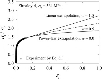
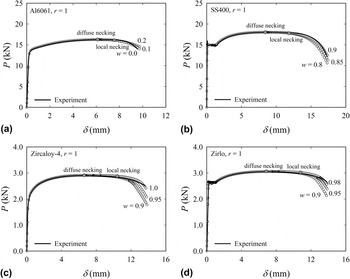
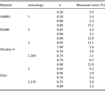
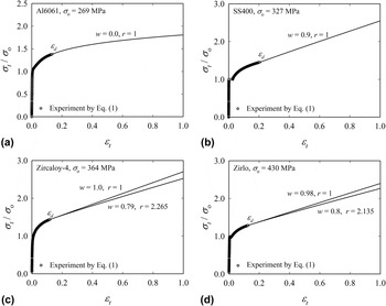
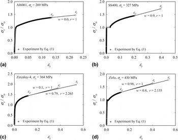
where σ_d and ε_d are true stress and true strain, respectively, at the point of diffuse necking. Note that setting w = 1 in Eq. (14) means bilinear and w = 0 power law behavior (Fig. 8). The weight factor w ∈ [0, 1] is then determined by minimizing the gap between experimental and numerical FE load–displacement curve. We skip the conversion of triaxial stress state to uniaxial stress state (i.e., the Bridgman correction) and directly fit tensile test data to analytical results by changing w (Fig. 9). For a given displacement, the gap between experimental load and FEA load reaches its maximum value close to the point of fracture. However, it is difficult to obtain the fracture displacement accurately from P–δ test data. We thus introduce an approximate fracture displacement δ_f which is about δ_f = 9.3 mm (Al6061), 17.4 mm (SS400), 13.9 mm (Zircaloy-4), and 14.2 mm (Zirlo) and determine w so that the load difference between experiment and analysis is less than 3% at δ_f; the obtained SS data are taken as the final SS data. Table IV lists the weight factor w and the corresponding load gap near the fracture point. When isotropic material behavior is assumed, the weights w for Al6061, SS400, Zircaloy-4, and Zirlo are 0.0, 0.90, 1.0, and 0.98, respectively. Corresponding SS curves are depicted in Fig. 10.

FIG. 8.

True SS curves from test and extrapolated one.

FIG. 9.

Load–displacement curves of four different specimens for various values of w for (a) Al6061, (b) SS400, (c) Zircaloy-4, and (d) Zirlo.

TABLE IV.

Comparison of maximum error for loads obtained from tensile test and FE analysis.

FIG. 10.

True SS curves for four different specimens for various values of w for (a) Al6061, (b) SS400, (c) Zircaloy-4, and (d) Zirlo.

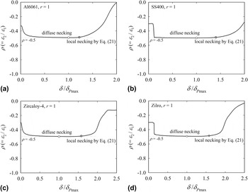
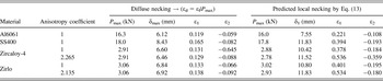
Figure 11 shows the change of minor-to-major strain ratio for each material. The strains at local necking (ε_l) obtained by Eq. (13) are 0.221, 0.394, 0.378, and 0.401 for Al6061, SS400, Zircaloy-4, and Zirlo, respectively (Table V). For isotropic materials, the theoretical local necking point based on Hill's theory is ε_l = 2n = 2ε₁|P _max. Since Al6061 obeys the power law (w = 0), the local necking point based on Hill's theory is 0.238. For Al6061, the difference between the strain calculated by Eq. (14) and the theoretical value is approximately 7%. On the contrary, Zirlo does not obey the power law (w = 1.0) and thus Hill's theory is not applicable. Figure 12 shows the final true SS curves up to the local necking point for the four materials.

FIG. 11.

The ratio of ε₂ to ε₁ versus displacement of (a) Al6061, (b) SS400, (c) Zircaloy-4, and (d) Zirlo.

TABLE V.

Obtained strains at diffusion and local necking points for four different specimens.

FIG. 12.

Modified true SS curve for (a) Al6061, (b) SS400, (c) Zircaloy-4, and (d) Zirlo.

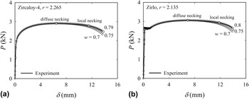
Material anisotropy affects the SS curves and the local necking point. Anisotropy coefficients are obtained from anisotropy tests on Zircaloy-4 and Zirlo. Anisotropy coefficients from tests with angular offset from the rolling direction are (r ₀ = 1.528, r ₄₅ = 2.506, r ₉₀ = 2.520 for Zircaloy-4) and (r ₀ = 2.247, r ₄₅ = 2.223, r ₉₀ = 1.846 for Zirlo). In the FE analysis, we use the normal anisotropy calculated by Eq. (10). Considering the anisotropy of both materials, the new weight factors w are found to be 0.79 and 0.80 for Zircaloy-4 (r = 2.265) and Zirlo (r = 2.135), respectively (Fig. 13). Local necking strains are 39% (Zircaloy-4; ε_l = 0.378| _{r = 1} → 0.536| _{r = 2.265}) and 33% (Zirlo: ε_l = 0.401| _{r = 1} → 0.534| _{r = 2.135}) higher than those obtained assuming isotropic material behavior [Table V and Figs. 12(c) and 12(d)].

FIG. 13.

Load–displacement curves of (a) Zircaloy-4 (r = 2.265) and (b) Zirlo (r = 2.135) for various values of w.

VI. DETERMINATION OF APPARENT FRACTURE STRAIN

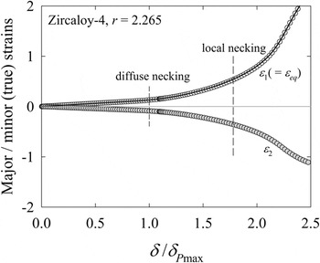
Figure 14 shows the changes of major and minor strain (ε₁, ε₂) with increasing displacement. ε₁ ( $\buildrel\textstyle.\over=$ equivalent strain, ε_eq) rises rapidly after the point of local necking. One way to obtain the fracture strain ε_f (or the fracture stress) is to measure the cross-section A _f at fracture [Eq. (2)]. However, after diffuse necking, the cross-section deviates from its initial rectangular shape, ^{Reference Zhang, Hauge, Odegard and Thaulow16} making the measurement of A _f difficult. Further, since the stress calculated by Eq. (2) is the mean stress corresponding to a triaxial stress state, a correction (such as the Bridgman correction) from triaxial stress to uniaxial stress state would be necessary.

FIG. 14.

Change of major and minor strains (ε₁ and ε₂) with displacement.

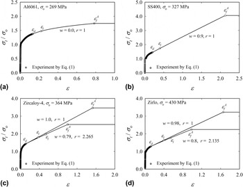
Consider the SS curve for anisotropic Zircaloy-4 (r = 2.265, w = 0.79) in Fig. 10(c), which is again shown in Fig. 15(a) as a dashed line (I). FE analysis based on the SS curve (I) in Fig. 15(a) yields the P–δ curve (dashed line I) in Fig. 15(b). In contrast to the experiment, the curve does not exhibit a pronounced load drop. Based on this observation, we suggest an SS curve that shows no hardening after a certain strain limit ε_L. Taking into account that strain limits should be larger than the local necking strain ε_l, we assume three hardening limits at 0.8, 0.9, and 1.0.

FIG. 15.

(a) σ_t–ε_t curves of Zircaloy-4 for three different ${\rm{\varepsilon }}_{\rm{f}}^A$ ; (b) P–δ curves for various hardening limit strains; and (c) enlargement of the load drop region of (b).

In Fig. 15(b), the experimental P–δ curve is shown together with those generated by FE analyses based on the four SS curves (dashed line I and solid lines II) in Fig. 15(a). All five P–δ curves show a similar run up to the point of sharp load drop. Taking a closer look at the region around that point [Fig. 15(c)], we find that when assuming ε_L = 1.0, the load drop point is the closest to experiment. Thus ε_L =1.0 may be taken as the apparent fracture strain ${\rm{\varepsilon }}_{\rm{f}}^A$ for Zircaloy-4 (note that ${\rm{\varepsilon }}_{\rm{f}}^A$ = ε₁ at δ_f). Having obtained ${\rm{\varepsilon }}_{\rm{f}}^A$ for the other three materials, we replot the true SS curves of Fig. 10 in Fig. 16, but now with nonhardening behavior after ${\rm{\varepsilon }}_{\rm{f}}^A$ . These types of SS curve are useful in, for instance, large deformation stamping.

FIG. 16.

Modified true SS curves up to apparent fracture strain for (a) Al6061, (b) SS400, (c) Zircaloy-4, and (d) Zirlo.

VII. CONCLUDING REMARKS

In this study, we developed a procedure to obtain accurate true SS data by tensile tests on plate specimens and FEA. In particular, we established a method to predict the strain at the onset of local necking in terms of the minor-to-major strain ratio and examined the influence of material anisotropy on the SS curve and the strain at local necking.

True SS data prior to diffuse necking were obtained from tensile tests while true SS data after diffuse necking were obtained by the triaxial-to-uniaxial stress conversion method proposed by Ling. Analytical load–displacement data were directly fit to tensile test data.

Due to the fact that fracture happens shortly after local necking without any further significant elongation, local necking was regarded as a valid upper limit of true SS curves. To find the onset of local necking, we observed the change of minor-to-major strain ratio |ρ| at the specimen center. The ratio |ρ| remains constant up to the local necking point and decays after local necking. Therefore, the local necking point was defined as the point where |ρ| drops suddenly; |ρ_local| was calculated based on the major strain and the minor-to-major strain ratio at maximum load. The major strain corresponding to |ρ_local| is considered the strain value at the onset of local necking.

A correction factor c was determined such that FEA local strains match theoretical values. The proposed method was validated by comparing the predicted local necking strains of materials obeying the power law with theoretical local necking strains. Thereafter, we determined the local necking strains for Al6061, SS400, Zircaloy-4, and Zirlo. The effects of anisotropic coefficients on true SS curves and local necking were discussed and it was found that when considering material anisotropy, the weight factor w decreases by approximately 20% and the local necking strain increases by approximately 40%; accounting for material anisotropy yielded more accurate true SS curves.

The major strain at the approximate fracture displacement was regarded as the apparent fracture strain. As a result, our method is not only useful for obtaining true SS curves but also to predict the point of local necking for nonpower law hardening materials. Furthermore, assuming nonhardening material behavior after apparent fracture strain can be a simple but an effective way of dealing with ductile fracture.