





1. Introduction
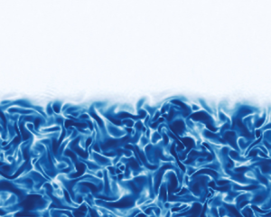
Turbulent flows are often bounded by regions of non-turbulent motion (Pope Reference Pope2000). Examples include virtually all canonical turbulent free-shear flows, i.e. turbulent mixing layers, turbulent jets and turbulent wakes, but the same is true of turbulent boundary layers. In these flows, the non-turbulent (NT) and turbulent (T) flow regions are separated by the turbulent/non-turbulent interface (TNTI), which is a very sharp and highly contorted layer (Bisset, Hunt & Rogers Reference Bisset, Hunt and Rogers2002; Westerweel et al. Reference Westerweel, Fukushima, Pedersen and Hunt2009; da Silva et al. Reference da Silva, Hunt, Eames and Westerweel2014). The sharpness of the TNTI is connected with an abrupt transition in the vorticity field observed between the T and NT flow regions, which can be defined for being regions with and without vorticity, respectively (Westerweel et al. Reference Westerweel, Fukushima, Pedersen and Hunt2005).
Whereas the vorticity and other quantities, e.g. passive scalar concentration, display abrupt changes across the TNTI layer (Watanabe et al. Reference Watanabe, Sakai, Nagata, Ito and Hayase2014; Silva & da Silva Reference Silva and da Silva2017), other quantities evolve smoothly across this layer, e.g. the mean and fluctuating velocity fields vary slowly across the TNTI layer, as shown by Taveira & da Silva (Reference Taveira and da Silva2013). In particular, while the cross Reynolds stresses,  $\langle u_i u_j \rangle$ with
 $i \ne j$, are rigorously zero in the NT flow region near the TNTI layer, the normal Reynolds stresses,
 $\langle u_i u_j \rangle$ with
 $i = j$, are typically very high in this region. For example, Westerweel et al. (Reference Westerweel, Fukushima, Pedersen and Hunt2009) and Taveira & da Silva (Reference Taveira and da Silva2013) have shown that the streamwise normal Reynolds stresses in the TNTI layer from a planar turbulent jet are already approximately one half their value inside the turbulent core region of the flow.
The fact that very important potential velocity fluctuations exist in the NT region close to the TNTI layer can be understood by the presence of both large- and small-scale vorticity structures in the T region bounding the TNTI layer. Indeed, it has been shown that these structures themselves define the geometry of the TNTI layer (da Silva et al. Reference da Silva, Hunt, Eames and Westerweel2014) and the intense potential velocity fluctuations observed in the NT region can be explained by the motion induced by these structures (da Silva, dos Reis & Pereira Reference da Silva, dos Reis and Pereira2011; Watanabe et al. Reference Watanabe, Jaulino, Taveira, da Silva, Nagata and Sakai2017).
The investigation of the potential velocity fluctuations bounding a TNTI layer began with the pioneering work of Phillips (Reference Phillips1955). Here we denote the fluctuating velocity vector field by  $u_i (\boldsymbol {x},t)$, with
 $i=1,2,3$, where
 $\boldsymbol {x}=x_i$ (
 $i=1,2,3$) and
 $t$ are the three spatial coordinates and the time, respectively, and the index
 $i=2$ corresponds to the direction normal to the TNTI layer. Here, use is made of the Reynolds decomposition, i.e. the total velocity field is the sum of the mean and fluctuating velocity fields, respectively
 $\langle U_i (\boldsymbol {x}) \rangle + u_i (\boldsymbol {x},t)$, where the brackets ‘
 $\langle \ \rangle$’ represent an averaging operation to be described later. By using a kinetic energy spectrum with an infrared (low wavenumber) region of the form
 $E(k) \sim k^{4}$, which is implied by assuming that
 $E(k)$ is differentiable at the origin, Phillips (Reference Phillips1955) was able to obtain asymptotic laws governing the profiles of all the second-order moments of the fluctuating velocity
 $\langle u_i u_j (x_2) \rangle$ (
 $i,j=1,2,3$) as a function of the distance from the TNTI layer,
 $x_2$, provided this distance is much bigger than the integral scale of turbulence,
 $x_2 \gg L$, e.g.
 $\langle u_1^{2} \rangle \sim x_2^{-4}$. He was also able to demonstrate other interesting results, e.g.
 $\langle u^{2}_2 (x_2) \rangle = \langle u^{2}_1 (x_2) \rangle + \langle u^{2}_3 (x_2) \rangle$.
By using rapid distortion theory (RDT), Carruthers & Hunt (Reference Carruthers and Hunt1986) were able to extend the relation derived by Phillips (Reference Phillips1955) for the entire range of coordinates  $x_2$, which allowed them to obtain the mean profiles of many important quantities in the NT region, such as the profile of the integral scale of turbulence. The analysis assumes that the NT region evolves in the absence of mean shear and, although the work focuses on the effects of stable stratification, the classical (Phillips Reference Phillips1955) results are recovered when considering no stratification. More recently, Teixeira & da Silva (Reference Teixeira and da Silva2012) used RDT to extend the analysis of the potential velocity fluctuations by considering the effects of a thin viscous layer roughly coinciding with the TNTI layer. While extending the results obtained by Phillips (Reference Phillips1955), both Carruthers & Hunt (Reference Carruthers and Hunt1986) and Teixeira & da Silva (Reference Teixeira and da Silva2012) recovered the asymptotic results of Phillips (Reference Phillips1955), such as the relation
 $\langle u^{2}_2 (x_2) \rangle = \langle u^{2}_1 (x_2) \rangle + \langle u^{2}_3 (x_2) \rangle$, which is independent of the shape of the kinetic energy spectrum assumed in the derivations.
The asymptotic laws governing the potential velocity fluctuations derived by Phillips (Reference Phillips1955) have also been observed in a number of experimental works such as in turbulent jets (Bradbury Reference Bradbury1965; Sunyach & Mathieu Reference Sunyach and Mathieu1969), turbulent wakes (Thomas Reference Thomas1973; Fabris Reference Fabris1979; Antonia, Shah & Browne Reference Antonia, Shah and Browne1987), turbulent mixing layers (Wygnanski & Fiedler Reference Wygnanski and Fiedler1970) and also in turbulent boundary layers (Bradshaw Reference Bradshaw1967; Kovasznay, Kibens & Blackwelder Reference Kovasznay, Kibens and Blackwelder1970).
Numerical verification has also been obtained in several works, such as in turbulent planar jets (Taveira & da Silva Reference Taveira and da Silva2013). Surprisingly, all these works claim to have recovered the asymptotic relations  $\langle u_1^{2} \rangle , \langle u_2^{2} \rangle , \langle u_3^{2} \rangle \sim x_2^{-4}$; however, it is important to stress that this law, like other similar laws derived by Phillips (Reference Phillips1955), is based on the assumed form of the kinetic energy spectrum in the infrared region (
 $E(k) \sim k^{4}$), also denoted as Batchelor spectrum (Davidson Reference Davidson2004), while, with the exception of Bradshaw (Reference Bradshaw1967), no mention of the form of the spectra in the infrared region is made in the experiments.
It is noteworthy that Phillips (Reference Phillips1955), Bradshaw (Reference Bradshaw1967), Carruthers & Hunt (Reference Carruthers and Hunt1986) and Teixeira & da Silva (Reference Teixeira and da Silva2012) all mention the fact that their theoretical results for the irrotational velocity fluctuations depend on the form of the kinetic energy spectrum at low wavenumbers, but they do not try to extend their results to different forms of the spectra. Nevertheless, it has been shown that spectra of the form  $E(k) \sim k^{2}$ (Saffman Reference Saffman1967), also denoted as Saffman spectrum (Davidson Reference Davidson2004), do arise in several turbulent flows. Spectra with the general form
 $E(k) \sim k^{n}$, in the infrared region, where
 $n$ is a constant, have also been assumed to exist in several other turbulent flows (Birkhoff Reference Birkhoff1954; Eyink & Thomson Reference Eyink and Thomson2000; Vassilicos Reference Vassilicos2011; Oberlack & Zieleniewicz Reference Oberlack and Zieleniewicz2013).
The present work uses RDT to generalise the analytical results obtained by Phillips (Reference Phillips1955), by considering turbulent flows where the kinetic energy spectrum in the infrared region follows the law  $E(k) \sim k^{2}$ (Saffman turbulence). For this case, and for large distances from the TNTI (
 $x_2 \gg L$), the velocity variance in the NT region evolves as
 $\langle u_i^{2} \rangle \sim x_2^{-3}$ (
 $i=1,2,3$), while the Taylor micro-scale
 $\lambda$ and viscous dissipation rate
 $\varepsilon$ evolve as
 $\langle \lambda \rangle \sim x_2$ and
 $\langle \varepsilon \rangle \sim x_2^{-5}$, respectively.
The new theoretical results are confirmed using several new direct numerical simulations (DNS) of shear-free turbulence (SFT), where a TNTI interface layer is generated in the absence of mean shear. Moreover, the effects of the Reynolds number and peak wavenumber are assessed, and it is shown that these results are robust and independent of these parameters. The new results are expected to be valid for other flow configurations, e.g. in the presence of mean shear, such as jets and wakes, provided the kinetic energy spectra in the turbulence region exhibits a Batchelor or a Saffman spectrum, because, as described above, the results of Phillips (Reference Phillips1955), which correspond to a Batchelor spectrum, have been observed in numerous flow configurations exhibiting mean shear.
This paper is organised as follows. The next section (§ 2) reviews the classical results obtained by Phillips (Reference Phillips1955) and extends them, using RDT, by considering an infrared kinetic energy spectrum with a form  $E(k) \sim k^{2}$. Section 3.1 describes the numerical methods, simulations and validation of the new simulations used in the present work. Section 4 assesses the new theoretical results obtained in this work. The paper ends with an overview of the main results of the paper (§ 5).
2. Analytical descriptions of the irrotational flow region
In this section, the classical theoretical results derived by Phillips (Reference Phillips1955) for the behaviour of the velocity fluctuations in the NT region near a TNTI layer are briefly reviewed and, by using RDT, these results are extended for the case of energy spectra obeying a power law of the form  $E(k) \sim k^{2}$ in the infrared region.
2.1. Phillips's asymptotic decay rates for the velocity fluctuations in the NT region
In the seminal work by Phillips (Reference Phillips1955), the problem of determining the velocity fluctuations in the irrotational flow region in the vicinity of a turbulent region was approached by considering a potential inviscid flow. One of the boundaries of the quiescent fluid domain was set as an infinite perturbation plane, with a fluctuating velocity field defined so as to satisfy a prescribed kinetic energy spectrum. Given the symmetry of the problem, tangential directions to the perturbation plane ( $x_1$ and
 $x_3$) are considered infinite. Phillips (Reference Phillips1955) thus created a model for the TNTI, where the effects of the perturbation plane in the irrotational flow domain are set by matching the normal velocity fluctuations at that plane. This model only allows for kinematic coupling between turbulent and non-turbulent regions, i.e. it precludes the prescription of any type of dynamical interaction between the two flow regions. Phillips (Reference Phillips1955) then showed that as the distance from the TNTI (
 $x_2$) increases, the importance of the larger wavenumbers is suppressed, so that the velocity fluctuations depend only on the shape of the infrared region of the spectrum at
 $x_2=0$. Specifically, the kinetic energy of the potential velocity fluctuations at a distance
 $x_2$ from the TNTI is (Phillips Reference Phillips1955),
 \begin{equation} \tfrac{1}{2} \langle \boldsymbol{u}^{2} (x_2) \rangle = \int \theta(k_1,k_3)\ \textrm{e}^{{-}2k_{13} x_2} \, {\textrm{d}}k_1\, {\textrm{d}}k_3, \end{equation}
where  $k_{13} = \sqrt {k_1^{2} + k_3^{2}}$ is the magnitude of the wavenumber vector
 $\boldsymbol {k_{13}} = (k_1,k_3)$ in planes
 $x_2 = \textrm {const.}$, and
 $\theta(k_1,k_3)$ is a two-dimensional spectrum of the normal velocity component
 $u_2 (x_1,0,x_3)$ defined by
 \begin{equation} {\theta}(k_1,k_3) = \frac{1}{(2{\rm \pi} )^{2}} \int \langle u_2 (x_1,0,x_3) u_2 (x_1',0,x_3') \rangle \, \textrm{e}^{-\textrm{i}\, \boldsymbol{k_{13}} \cdot \boldsymbol{r} } \, {\textrm{d}} \boldsymbol{r}, \end{equation}
with  $\boldsymbol {r} = (r_1,r_3) = (x_1'-x_1,x_3'-x_3)$. The two-dimensional kinetic energy spectrum at a distance
 $x_2$ from the TNTI is given by
 \begin{equation} E(k_{13}, x_2) = \int \theta(k_1,k_3)\ \textrm{e}^{{-}2k_{13} x_2} \, {\textrm{d}}S(k_{13}) = E_0(k_{13})\ \textrm{e}^{{-}2k_{13} x_2}, \end{equation}
where  ${\textrm {d}}S(k_{13})$ is the arc for the integration over circular shells with radius
 $k_{13}$, while
 $E_0(k_{13})$ is the kinetic energy spectrum at the interface (
 $x_2=0$). To compute the irrotational velocity fluctuations, Phillips (Reference Phillips1955) uses a spectrum
 ${\theta }(k_1,k_3)$ with the form
 \begin{equation} \theta(k_1, k_3) = k_i k_j \theta^{ij} + O(k_{13}^{3}), \end{equation}
where  $\theta ^{ij}$ is a constant, which is reminiscent of the usual form of the three-dimensional kinetic energy spectrum given by Batchelor (Reference Batchelor1953) as
 \begin{equation} E(k) = C k^{4} + O(k^{6}), \end{equation}
where  $k = (k_1^{2} + k_2^{2} +k_3^{3})^{1/2}$ is the magnitude of the three-dimensional wavenumber vector,
 $\boldsymbol {k} = (k_1,k_2,k_3)$, and
 $C$ is a constant. By replacing (2.4) into (2.1), Phillips (Reference Phillips1955) arrives at
 \begin{equation} \tfrac{1}{2} \langle \boldsymbol{u}^{2} \rangle \sim x_2^{{-}4}, \end{equation}
which is then generalised into
 \begin{equation} \langle u_i^{2} \rangle \sim x_2^{{-}4}, \quad \textrm{for } i=1,2, \textrm{ or } 3. \end{equation}
Phillips (Reference Phillips1955) also showed that the potential velocity fluctuations obey the relation
 \begin{equation} \langle u^{2}_2 (x_2) \rangle = \langle u^{2}_1 (x_2) \rangle + \langle u^{2}_3 (x_2) \rangle, \end{equation}
and that all the cross stresses are zero, e.g.  $\langle u_1 u_2 (x_2) \rangle = 0$. Additionally, using relations independent of the shape of the energy spectra (Phillips Reference Phillips1955; Teixeira & da Silva Reference Teixeira and da Silva2012)
 \begin{equation} \left\langle \left(
\frac{ \partial u_i }{ \partial x_2 } \right)^{2}
\right\rangle = \left\langle \left( \frac{ \partial u_i }{
\partial x_1 } \right)^{2} \right\rangle + \left\langle
\left( \frac{ \partial u_i }{ \partial x_3 } \right)^{2}
\right\rangle , \end{equation}
and
 \begin{equation} \left\langle \left(
\frac{ \partial u_2 }{ \partial x_i } \right)^{2}
\right\rangle = \left\langle \left( \frac{ \partial u_1 }{
\partial x_i } \right)^{2} \right\rangle + \left\langle
\left( \frac{ \partial u_3 }{ \partial x_i } \right)^{2}
\right\rangle , \end{equation}
together with
 \begin{equation} \varepsilon = \nu \left[ \langle \omega^{2} \rangle + 2 \frac{ \partial^{2} \langle u^{2}_2 \rangle}{ \partial x_2^{2}} \right], \end{equation}
where  $\nu$ is the kinematic viscosity and
 $\langle \omega ^{2} \rangle$ is the mean enstrophy in the turbulence region, the following scaling laws (inside the irrotational region) for the Taylor micro-scale can be obtained:
 \begin{equation} \lambda_i \sim x_2 \quad (i=1,2,3), \end{equation}
where the Taylor micro-scale is defined by
 \begin{equation} \lambda_i = \sqrt{\frac{\langle u_i^{2} \rangle}{\langle (\partial u_i / \partial x_i)^{2} \rangle}} (\textrm{no summation}) \quad (i=1,2,3), \end{equation}
which implies that the viscous dissipation rate follows the law
 \begin{equation} \varepsilon \sim x_2^{{-}6}. \end{equation}
This completes the scaling relations obtained by Phillips (Reference Phillips1955), while assuming the form of the two-dimensional spectrum of the normal velocity component described in (2.4).
The dynamical interaction between the turbulent and non-turbulent flow regions, not accounted for by Phillips (Reference Phillips1955), is included by Carruthers & Hunt (Reference Carruthers and Hunt1986), where pressure interactions are considered in a stably stratified non-turbulent region, and by Teixeira & da Silva (Reference Teixeira and da Silva2012), where viscous effects in the vicinity of the TNTI are included. These works resorted to using RDT, which is valid for time intervals much smaller than the characteristic time scale of nonlinear interactions. The introduction of dynamical interactions between the turbulent and non-turbulent regions, by coupling the T and NT regions in a physically consistent way, preserves the asymptotic results at large distances from the interface, typically for distances from the TNTI larger than the integral scale of turbulence  $x_2 \gg L$ (Carruthers & Hunt Reference Carruthers and Hunt1986; Teixeira & da Silva Reference Teixeira and da Silva2012). Similarly, Teixeira & da Silva (Reference Teixeira and da Silva2012) show that the effects of viscosity, which are restricted in that case to a very thin layer within the TNTI, quickly fade away from this interface, in agreement with (2.1) from Phillips (Reference Phillips1955), which implies that the velocity fluctuations far from the TNTI depend only on the largest scales of the flow within the turbulent region.
2.2. Extending the classical results for an infrared energy spectrum with  $E(k) \sim k^{2}$

As mentioned in the introduction, while Phillips (Reference Phillips1955), Bradshaw (Reference Bradshaw1967), Carruthers & Hunt (Reference Carruthers and Hunt1986) and Teixeira & da Silva (Reference Teixeira and da Silva2012) mention the dependency of the asymptotic behaviour laws for the irrotational velocity fluctuations on the shape of the kinetic energy spectrum at lower wavenumbers, they did not extend their results for a general kinetic energy spectrum of the form  $E(k) \sim k^{n}$, even though turbulent flows with
 $n=4$ (Batchelor turbulence) and
 $n=2$ (Saffman turbulence), as well as other cases, have been reported (Davidson Reference Davidson2004). This generalisation for the case
 $n=2$ is done in this section.
The expression for the variance of the tangential velocity fluctuations in the irrotational part of the flow was given by Teixeira & da Silva (Reference Teixeira and da Silva2012) (their (3.18)) as
 \begin{equation} \langle u_1^{2} (x_2) \rangle = \frac{1}{16 {\rm \pi}} \int_0^{2{\rm \pi} } \int_0^{+\infty} \int_{-\infty}^{+\infty} \frac{E(k)}{k^{4}} k_{13}^{3} \cos^{2} \alpha \, \textrm{e}^{{-}2 k_{13} x_2} \, {\textrm{d}}k_2\, {\textrm{d}}k_{13} \, {\textrm{d}} \alpha,\end{equation}
where  $k_{13}=(k_1^{2}+k_3^{2})^{1/2}$,
 $k_1$ and
 $k_3$ are the components of the wavenumber in the directions tangential to the TNTI, and
 $k_2$ is the component of the wavenumber in the normal direction. Here
 $\alpha$ is the angle made by
 $(k_1,k_3)$. Note that in (2.15), cylindrical coordinates were adopted for the integrals. This expression is valid for any energy spectrum
 $E(k)$, with
 $k = (k_1^{2} + k_2^{2} + k_3^{2})^{1/2} = (k_{13}^{2} + k_2^{2})^{1/2}$.
In Teixeira & da Silva (Reference Teixeira and da Silva2012), an exponential energy spectrum with a power law of  $k^{4}$ in the infrared region was considered, namely
 \begin{equation} E(k)= \frac{1}{(2 {\rm \pi})^{1/2}} q^{2} \lambda_\infty ( k \lambda_\infty )^{4} \, \textrm{e}^{(-{1}/{2}) (k \lambda_\infty )^{2}},\end{equation}
(their (2.26)), where  $q$ is the root mean square (RMS) velocity in the homogeneous turbulence, i.e. the other (turbulent) side of the TNTI, and
 $\lambda _\infty$ is the corresponding Taylor micro-scale. An energy spectrum of the same type, but where the power law in the infrared region is
 $k^{2}$, takes the form
 \begin{equation} E(k)=\frac{9}{5} \left( \frac{3}{10 {\rm \pi}} \right)^{1/2} q^{2} \lambda_\infty ( k \lambda_\infty )^{2} \, \textrm{e}^{(-{3}/{10}) (k \lambda_\infty )^{2}}.\end{equation}
Note that both the coefficient that defines the amplitude of the spectrum and that in the exponential have different values from those in (2.16), because the spectrum must be consistent with the definitions of the RMS velocity and Taylor micro-scale. Another property of the exponential spectra of the form (2.17) is that their integral length scale  $L_\infty$ and Taylor micro-scale
 $\lambda _\infty$ are related by a fixed factor. For (2.16), the relation is
 $L_\infty =({\rm \pi} /2)^{1/2} \lambda _\infty$ (as noted by Teixeira & da Silva Reference Teixeira and da Silva2012) and for (2.17),
 $L_\infty =(27 {\rm \pi}/40)^{1/2} \lambda _\infty$.
If (2.17) is used in (2.15), the integration over the angle  $\alpha$ may be performed analytically, because
 $E(k)$ does not depend on
 $\alpha$, which yields a multiplication by a factor of
 ${\rm \pi}$. The integration over the wavenumber
 $k_2$ is less immediate, and yields
 \begin{equation} \langle u_1^{2} (x_2) \rangle = \frac{9}{80} \left( \frac{3 {\rm \pi}}{10} \right)^{1/2} q^{2} \int_0^{+\infty} \left[ 1 - \varPhi \left( \sqrt{\frac{3}{10}} k_{13}^{\prime} \right) \right] k_{13}^{\prime 2} \, \textrm{e}^{{-}2 k_{13}^{\prime} (x_2/\lambda_\infty)} \, {\textrm{d}}k_{13}^{\prime}, \end{equation}
where  $k_{13}^{\prime }=k_{13} \lambda _\infty$ and
 $\varPhi$ is the error function. This expression is considerably more complicated than that obtained by Teixeira & da Silva (Reference Teixeira and da Silva2012) for (2.16), but its asymptotic behaviour as
 $x_2 \rightarrow \infty$ can be obtained in a similar way, resulting in some simplifications. Namely, the contributions to the integral over
 $k_{13}$ when
 $x_2 \gg 1$ come mainly from small values of
 $k_{13}$. When this approximation is made, the error function reduces approximately to zero, and (2.18) simplifies to
 \begin{equation} \langle u_1^{2} (x_2) \rangle \sim \frac{9}{320} \left( \frac{3 {\rm \pi}}{10} \right)^{1/2} \frac{q^{2}}{(x_2/\lambda_\infty)^{3}}. \end{equation}
Note that the proportionality coefficients present in this expression depend on the shape of the spectrum (2.17), more specifically on the constants included in its definition, but the type of asymptotic variation with  $x_2$ only relies on the type of dependence of the spectrum at small wavenumbers. This was also the case with the asymptotic expression obtained by Teixeira & da Silva (Reference Teixeira and da Silva2012) for a spectrum proportional to
 $k^{4}$ in the infrared region, which yielded instead
 \begin{equation} \langle u_1^{2} (x_2) \rangle \sim \frac{3}{128} \frac{q^{2}}{(x_2/\lambda_\infty)^{4}}, \end{equation}
(their (3.20)). Because the relation stating that  $\langle u_2^{2} (x_2) \rangle = 2 \langle u_1^{2} (x_2) \rangle$ remains valid for any energy spectrum, it is straightforward to obtain
 $\langle u_2^{2} (x_2) \rangle$ from (2.19) (or (2.20)).
By using the relations presented in § 2.1, the asymptotic power law governing the viscous dissipation rate can be easily obtained as
 \begin{equation} \varepsilon = 2 \nu \frac{\partial^{2} \langle u_2^{2} \rangle}{\partial x_2^{2}} \sim \frac{27}{20} \left( \frac{3 {\rm \pi}}{10} \right)^{1/2} \nu \frac{q^{2}}{\lambda_\infty^{2}} \frac{1}{(x_2/\lambda_\infty)^{5}} = \frac{9}{100} \left( \frac{3 {\rm \pi}}{10} \right)^{1/2} \frac{\varepsilon_\infty}{(x_2/\lambda_\infty)^{5}},\end{equation}
where, in the last equality, the fact that the dissipation rate in the isotropic turbulence is defined as  $\varepsilon _\infty = 15 \nu q^{2}/\lambda _\infty ^{2}$ has been used. This should be compared with the corresponding relation obtained by Teixeira & da Silva (Reference Teixeira and da Silva2012), which can be written as
 \begin{equation} \varepsilon = \frac{1}{8} \frac{\varepsilon_\infty}{(x_2/\lambda_\infty)^{6}},\end{equation}
(their (3.22)).
The Taylor micro-scale is defined as (see (3.27) of Teixeira & da Silva Reference Teixeira and da Silva2012)
 \begin{equation} \lambda_1 = \left[ \frac{\langle u_1^{2} \rangle}{\left\langle \left( \dfrac{\partial u_1}{\partial x_1} \right)^{2} \right\rangle} \right]^{1/2}.\end{equation}
Its behaviour is controlled by the behaviour of  $\langle (\partial u_1/\partial x_1)^{2} \rangle$ (in addition to that of
 $\langle u_1^{2} \rangle$). Because differentiation with respect to
 $x_1$ corresponds in Fourier space to multiplication by
 $k_1$, by analogy with (2.15),
 $\langle (\partial u_1/\partial x_1)^{2} \rangle$ can be expressed as
 \begin{equation} \left\langle \left( \frac{\partial u_1}{\partial x_1} \right)^{2} \right\rangle = \frac{1}{16 {\rm \pi}} \int_0^{2 {\rm \pi}} \int_0^{+\infty} \int_{-\infty}^{+\infty} \frac{E(k)}{k^{4}} k_{13}^{5} \cos^{4} \alpha \, \textrm{e}^{{-}2 k_{13} x_2} \, {\textrm{d}}k_2\, {\textrm{d}}k_{13} \, {\textrm{d}} \alpha.\end{equation}
Following the same procedure as before, the integration over  $\alpha$ is straightforward, corresponding to multiplication by
 $3 {\rm \pi}/4$, and the integration over
 $k_2$ proceeds identically as in (2.15), using also (2.17). Taking again the limit
 $x_2 \rightarrow \infty$, for which contributions to the integral come mostly from small
 $k_{13}$, we obtain
 \begin{equation} \left\langle \left( \frac{\partial u_1}{\partial x_1} \right)^{2} \right\rangle \sim \frac{81}{1280} \left( \frac{3 {\rm \pi}}{10} \right)^{1/2} \frac{q^{2}}{\lambda_\infty^{2}} \frac{1}{(x_2/\lambda_\infty)^{5}}.\end{equation}
Then, using the definition (2.23), and also (2.25) and (2.19), the Taylor micro-scale can be shown to take the asymptotic form for  $x_2 \rightarrow \infty$ as
 \begin{equation} \lambda_1 \sim \tfrac{2}{3} x_2.\end{equation}
This result shows that the Taylor micro-scale increases linearly from the TNTI into the irrotational flow region, which has the same qualitative asymptotic behaviour for the energy spectrum (2.17) as the expression obtained by Teixeira & da Silva (Reference Teixeira and da Silva2012) for the energy spectrum (2.16), namely
 \begin{equation} \lambda_1 \sim \left( \frac{32}{135} \right)^{1/2} x_2,\end{equation}
(their (3.29)).
2.3. Effect of the form of the kinetic energy spectrum in the new theoretical results
It is well known that the shape of the initial kinetic energy spectrum largely determines the temporal evolution of decaying isotropic turbulence (Davidson Reference Davidson2004). Moreover, as described above, the spectrum also has a crucial effect on the statistics of the potential velocity fluctuations in the irrotational region near a TNTI, as shown in (2.15). However, it is often argued that the asymptotic behaviour of the velocity fluctuations in the NT region depend only on the infrared region of the kinetic energy spectrum, which is assumed to follow a power law  $E(k) \sim k^{n}$ for
 $k<k_p$, because the higher wavenumbers
 $k>k_p$ of the energy spectra are modulated by the increase in the distance to the TNTI, as shown in (2.3). Therefore, it is important to insure that a particular shape of the kinetic energy spectra at high wavenumbers (
 $k>k_p$) does not affect the present theoretical results.
To assess this, we employ a simple model spectrum defined by Pope (Reference Pope2000),
 \begin{equation} E(k) = C_k \varepsilon^{2/3}\,f_{k_p}\,f_{k_\eta} k^{-{5}/{3}}, \end{equation}
where  $C_k=1.5$ is the Kolmogorov constant, with
 \begin{equation} f_{k_p} = \left\{ \frac{k/k_p}{[(k/k_p)^{2} + c_{k_p}]^{1/2}}\right\}^{{5}/{3} + n}, \end{equation}
and
 \begin{equation} f_{k_\eta} = \exp \{ -\beta [ [ (k/k_\eta)^{4} + c_{k_\eta}^{4} ]^{1/4} - c_{k_\eta} ] \}, \end{equation}
where  $k_p$ is again the peak wavenumber,
 $k_\eta$ is a dissipation scale wavenumber, and the parameters
 $\beta$,
 $c_{k_p}$ and
 $c_{k_\eta }$ are chosen for the spectrum to represent fully-developed isotropic turbulence at high turbulent Reynolds number
 $Re_{\lambda }$. Specifically, these parameters were set to
 $\beta = 5.2$,
 $c_{k_p} = 6.78$ and
 $c_{k_\eta } = 0.40$ (Pope Reference Pope2000).
The model spectrum defined by (2.28) allows an assessment of the dependence of the asymptotic mean profiles of kinetic energy on the integral length scale of turbulence, which is assumed to be  $L = k_p^{-1}$, and also on the power law of the infrared kinetic energy spectrum
 $n$. Moreover, by using distinct values of the ratio
 $k_\eta /k_p$, the dependence of the results on
 $Re_{\lambda }$ can be explored.
We start this analysis by comparing the results obtained from integrating the equation
 \begin{equation} \langle u_1^{2} (x_2) \rangle = \tfrac{1}{16} \int_0^{{\rm \pi} } \int_0^{+\infty} E(k) \sin^{3} \theta \ \textrm{e}^{{-}2 k \sin \theta x_2} \, {\textrm{d}}k \, {\textrm{d}} \theta,\end{equation}
which is the same as (2.15), but with the integral expressed in spherical polar coordinates instead of cylindrical coordinates (Teixeira & da Silva Reference Teixeira and da Silva2012), using (i) the form of the initial energy spectrum employed in the DNS of decaying homogeneous isotropic turbulence (DHIT), (3.1) shown in the next section, and (ii) the spectrum given by (2.28) reproducing a Batchelor ( $n=4$) or a Saffman (
 $n=2$) spectrum.
Figure 1 shows the resulting profiles of  $\langle u_i u_i \rangle$ as a function of the distance (
 $x_2-x_2^{I}$) from a particular surface within the TNTI layer – the so-called irrotational boundary (IB) – which is the surface separating the turbulent and non-turbulent flow regions, which is located at
 $x_2 = \pm x_2^{I}$. The profiles of
 $\langle u_i u_i \rangle$ have been obtained by integrating (2.31) using the two expressions for
 $E(k)$, i.e. using (2.28) and (3.1). For the integration of (2.28), we prescribed
 $k_p=80$ and
 $k_\eta = 8/3 \times 10^{5}$. It is clear that no difference is observed in the resulting power laws for the kinetic energy decay rate in both cases, because we recover
 $\langle u_i u_i \rangle \sim x_2^{- 3}$ and
 $\langle u_i u_i \rangle \sim x_2^{-4}$ for
 $n=2$ and
 $n=4$, respectively, which is equal to the asymptotic power laws obtained when
 $E(k) \sim k^{n}$ is used to analytically integrate (2.31).
Profiles of  $\langle u_i u_i \rangle$ as function of the distance from the TNTI layer (
 $x_2$) obtained though numerical integration of (2.31) by using the initial spectrum used in the DNS ((3.1)), solid lines; and that defined in (2.28), dashed lines; for a Batchelor spectrum (
 $n=4$) and a Saffman spectrum (
 $n=2$). In all cases,
 $k_p = 80$ and
 $k_\eta = 8/3 \times 10^{5}$. The mean profiles of kinetic energy
 $\langle u_i u_i \rangle$ are normalised by their value at the irrotational boundary (IB) which is the surface separating the turbulent and non-turbulent flow regions, and is located at
 $x_2 = \pm x_2^{I}$, while the distance from the IB (
 $x_2-x_2^{I}$) is normalised by the integral scale of turbulence assumed to be
 $L = k_p^{-1}$.

Figure 2 shows the effects of the turbulent Reynolds number on the kinetic energy decay rates in the non-turbulent flow region. Notice that this is equivalent to assessing the effects of the size of the inertial range region of the kinetic energy spectrum  $k_p < k< k_{\eta }$. Figure 2(a) shows the spectra given by (2.28) while figure 2(b) shows the profiles of
 $\langle u_i u_i \rangle$ in the non-turbulent region resulting from numerical integration of these spectra by solving (2.31). Different input parameters are used for the spectra. We fix
 $k_p=80$ and vary the dissipation wavenumber by using
 $k_{\eta } = 1/3\times 10^{4}$,
 $8/3\times 10^{5}$ and
 $8/3 \times 10^{6}$, which correspond to
 $Re_{\lambda } \sim 31$,
 $576$ and
 $2674$, respectively. The Reynolds number
 $Re_\lambda$ was estimated by taking
 $k_p \approx L^{-1}$,
 $k_\eta \approx \eta ^{-1}$ and by using the following relations for isotropic turbulence (Pope Reference Pope2000),
 \begin{equation} \frac{k_p}{k_\eta} \sim \frac{\eta}{L} \approx Re^{-{3}/{4}}_L, \end{equation}
and
 \begin{equation} Re_\lambda = ( \tfrac{20}{3} Re_L )^{1/2}. \end{equation}
Effect of the Reynolds number, represented by the size of the wavenumber range between  $k_p < k < k_{\eta }$, and the profiles of
 $\langle u_i u_i \rangle$ in the non-turbulent region obtained by integrating (2.31) with the spectra given by (2.28) with varying input parameters, for both
 $n=2$ and
 $n=4$. All spectra have
 $k_p=80$, where solid and dashed lines correspond to
 $n=2$ and
 $n=4$, respectively. The values of
 $k_{\eta }$ used are
 $1/3\times 10^{4}$,
 $8/3\times 10^{5}$ and
 $8/3 \times 10^{6}$, which correspond to
 $Re_{\lambda }$ of
 $31$,
 $576$ and
 $2674$, respectively. (a)
 $E(k)$ defined by (2.28) and (b)
 $\langle u_i u_i (x_2) \rangle$ obtained by integrating (2.31).

For low Reynolds numbers ( $Re_{\lambda } \sim 31$), which are similar to those of the DNS used in the present work, the form of the spectrum resembles that used to start the present DNS of DHIT, while the other cases clearly resemble spectra from high-Reynolds-number turbulence, where the values of
 $k_\eta$ were chosen to obtain
 $Re_\lambda$ differing by one order of magnitude (Pope Reference Pope2000). It is clear that the magnitude of the Reynolds number, or equivalently the extent of the wavenumber region as
 $k_p < k< k_{\eta }$, does not alter the scaling laws for the non-turbulent profiles of
 $\langle u_i u_i \rangle$ obtained from (2.31). This result justifies the use of DNS of DHIT with relatively low
 $Re_{\lambda }$ as a valid method to explore the asymptotic behaviour of the velocity fluctuations in the irrotational region.
The effect of the spectrum peak  $k_p$ on the asymptotic decay laws of the kinetic energy in the non-turbulent region is investigated in figure 3, which shows the mean profiles of
 $\langle u_i u_i \rangle$ in the non-turbulent region resulting from the numerical integration of (2.31), using (2.28) as the input spectrum for several values of
 $k_p$, specifically, we use
 $k_p = 3$,
 $5$,
 $10$ and
 $20$. As in the previous figure, both the cases of
 $n=2$ and
 $n=4$ are considered. As the value of
 $k_p$ increases, and therefore the integral scale
 $L$ decreases, the power law behaviour in the profiles of velocity variance
 $\langle u_i u_i \rangle$ begins closer to the interface (
 $x_2=0$) (figure 3a). Interestingly, when the normal distance
 $x_2$ is normalised by
 $k_p$, all the mean profiles of
 $\langle u_i^{2} \rangle$ collapse (figure 3b). Because the integral length scale of turbulence is assumed to be
 $L \sim k_p^{-1}$, this shows that the power law appears whenever
 $x_2 > L$, as expected; however, in no way does the prescribed value of
 $k_p$ affect the decay rate of the power laws
 $\langle u_i u_i \rangle \sim x_2^{-4}$ and
 $\langle u_i u_i \rangle \sim x_2^{-3}$ obtained for
 $n=4$ and
 $n=2$, respectively.
Effect of the peak wavenumber  $k_p$ on the profiles of
 $\langle u_i u_i \rangle$ in the non-turbulent region of the SFT simulations, obtained by integrating (2.31) with spectra given by (2.28), for both
 $n=2$ and
 $n=4$, where
 $k_p$ is varied as
 $k_p = 3$,
 $5$,
 $10$ and
 $20$: (a) using the normal distance
 $x_2$ without any normalisation (the arrow indicates increasing values of
 $k_p$); (b) normalising
 $x_2$ with the peak wavenumber
 $k_p$.

3. Direct numerical simulations
This section describes the numerical methods employed to carry out all the simulations analysed in the present work. The work relies on DNS of two flow configurations: (i) DHIT and (ii) SFT, where a turbulent front evolves into a quiescent (non-turbulent) flow region in the absence of mean shear.
3.1. Numerical methods
All the simulations employ the same code, which is an in-house Navier–Stokes solver that uses the classical pseudo-spectral methods (collocation method) for spatial discretisation (Canuto et al. Reference Canuto, Hussaini, Quarteroni and Zang1987), and a three-step third-order explicit Runge–Kutta scheme for the temporal advancement (Williamson Reference Williamson1980). The simulation domain is a triple periodic cube with sides equal to  $2 {\rm \pi}$ and the simulations are fully de-aliased using the
 $2/3$ rule. The computational grid is uniform and isotropic (
 ${\rm \Delta} x_1={\rm \Delta} x_2 = {\rm \Delta} x_3$) with
 $N_1 \times N_2 \times N_3$ collocation points, where
 $N_1 = N_2 = N_3$. More details on this code can be found in Silva, Zecchetto & da Silva (Reference Silva, Zecchetto and da Silva2018) and references therein.
3.2. Direct numerical simulations of DHIT and SFT
In the present work, we have carried out two DNS of DHIT. Both simulations use a total of  $N_1 \times N_2 \times N_3 = 1024 \times 1024 \times 1024$ collocation points along the
 $x_1$,
 $x_2$ and
 $x_3$ directions, respectively, and the kinematic viscosity is equal to
 $\nu = 2.67\times 10^{-4}$.
The two simulations basically differ in the details of the initial velocity field, obtained from a random number generator, which creates a divergent-free velocity field with initial variance equal to  $\langle u^{2}_1 \rangle = \langle u^{2}_2 \rangle = \langle u^{2}_3 \rangle = 1$ and a prescribed kinetic energy spectrum with the form
 \begin{equation} E(k) \sim k^{n} \ \textrm{e}^{{-}2 ( {k}/{k_p})^{2}}, \end{equation}
where  $k_p$ defines the peak wavenumber while
 $n$ controls the slope in the low-wavenumber (infrared) region (Ishida, Davidson & Kaneda Reference Ishida, Davidson and Kaneda2006). We designate the two DHIT simulations by
 $K4$ and
 $K2$, where the parameter
 $n$ is set to
 $n=4$ (Batchelor turbulence, Batchelor Reference Batchelor1953) and
 $n=2$ (Saffman turbulence, Saffman Reference Saffman1967), respectively, while the peak wavenumber is located at
 $k_p=30$ for both simulations. Figure 4 shows the initial kinetic energy spectrum for the two simulations, with the infrared slopes of
 $n=2$ and
 $n=4$ for
 $K2$ and
 $K4$, respectively.
Initial kinetic energy spectrum for the two DNS of DHIT used in the present work. Here  $K2$ and
 $K4$ correspond to the cases where the parameter
 $n$ in (3.1) is set to
 $2$ and
 $4$, respectively.

As in Ishida et al. (Reference Ishida, Davidson and Kaneda2006), we define a Reynolds number based on the integral scale of turbulence, which is assumed to be equal to the peak wavenumber  $L = k_p^{-1}$. This Reynolds number is defined as
 $Re_{k_p} = \langle u^{2} \rangle ^{1/2}/(k_p \nu )$ and, similarly in the following discussion, the time is normalised by the initial integral length scale turnover time
 $T_{k_p} = 1 / ( \langle u^{2} \rangle ^{1/2} k_p )$, i.e.
 $\tau =t/T_{kp}$. The initial Reynolds number for both simulations is equal to
 $Re_{k_p} =125$, as in the DHIT simulations of Ishida et al. (Reference Ishida, Davidson and Kaneda2006).
As shown in Ishida et al. (Reference Ishida, Davidson and Kaneda2006), to preserve the slope of the kinetic energy spectrum at low wavenumbers during the kinetic energy decay phase, the initial spectrum peak must be  $k_p > 20$. Ishida et al. (Reference Ishida, Davidson and Kaneda2006) also show that to attain the correct (theoretical) kinetic energy decay rates in DNS of DHIT, the Reynolds number must be at least
 ${Re}_{k_p} > 100$. These constraints are both fulfilled with the values of
 $Re_{k_p} =125$ and
 $k_p=30$ used in the present simulations. Moreover, the ratio of the maximum effective wavenumber
 $k_{max}$ and the peak wavenumber is
 $k_{max}/k_p=12$. This choice allows maximising the Reynolds number
 ${Re}_{k_p}$, while keeping the appropriate resolution. Starting with the initial conditions described above, each DHIT simulation follows the typical evolution described in many previous works (e.g. Ishida et al. Reference Ishida, Davidson and Kaneda2006). Initially, enstrophy increases with time as the kinetic energy spectrum develops, which increases the range of active wavenumbers, until a maximum (
 $\tau _{\omega }$, enstrophy peak) is attained, which is then followed by a slow decay. As will be shown in the following for both simulations, the rates of kinetic energy decay
 $\langle u^{2} \rangle \sim \tau ^{-m}$ recover the expected theoretical values, with
 $m=10/7$ and
 $m=6/5$ for the
 $K4$ and
 $K2$ simulations, respectively, after the enstrophy peak is attained.
From these two DHIT simulations, we generate DNS of SFT, where a turbulent front, which separates the turbulent and non-turbulent flow regions, evolves in the absence of mean shear. The procedure to obtain the SFT simulations has been described in several papers (Perot & Moin Reference Perot and Moin1995; Cimarelli et al. Reference Cimarelli, Cocconi, Frohnapfel and Angelis2015; Silva et al. Reference Silva, Zecchetto and da Silva2018) and so is only briefly outlined here.
Each SFT simulation starts from the velocity field obtained at a given time  $\tau =\tau _{SFT}$ from one of the DHIT simulations, where
 $\tau _{SFT}$ is always taken at a time after the enstrophy peak,
 $\tau _{SFT} > \tau _{\omega }$. At the selected time instant of the desired DHIT simulation, the velocity in the central domain region
 $- H/2 \leqslant x_2 \leqslant H/2$ is preserved, while the velocity in the remaining domain is set to zero, where
 $H$ is a parameter defining the width of the initial turbulent region. This is done through the convolution of the velocity field with a hyperbolic tangent profile (Cimarelli et al. Reference Cimarelli, Cocconi, Frohnapfel and Angelis2015; Silva et al. Reference Silva, Zecchetto and da Silva2018), which creates an initial SFT flow where turbulent (
 $H/2 \leqslant x_2 \leqslant H/2$) and non-turbulent (
 $x_2<-H/2 \wedge x_2>H/2$) flow regions are separated by a turbulent/non-turbulent interface. Each SFT then evolves for a few time iterations, whereby the initial isotropic turbulence flow region spreads into the irrotational (quiescent) region, in the absence of mean shear. Therefore, two distinct (upper and lower) TNTI layers develop within the computational domain as the turbulence slowly decays within the core of the turbulent region.
Several widths of the initial turbulence region  $H$ were tested to determine the influence of the hyperbolic tangent profile convolution on the shape of the resulting kinetic energy spectra. It was found that the effects of the hyperbolic tangent convolution were minimised with
 $H/2{\rm \pi} \approx 1/5$. It is important to maximise both the size of the initial turbulent region
 $H$, so that the large scales of motion remain unaffected, and the size of the non-turbulent region (
 $2{\rm \pi} -2H$) to ensure that it is not affected by the (periodic) boundary conditions. Several numerical experiments then led to the optimal ratio
 $H/2{\rm \pi} \approx 1/5$ used here. In this process, we also confirmed the need to use a size of the turbulent region with at least
 $H \gtrsim 4 L$, as described by Cimarelli et al. (Reference Cimarelli, Cocconi, Frohnapfel and Angelis2015) (we are using
 $H \gg 4 L$). Moreover, the adaptation of the irrotational flow region was found to require only four time steps, which correspond to
 $1.84 \tau _{\eta }$ and
 $1.56 \tau _{\eta }$ for the simulations
 $K2$ and
 $K4$, respectively, where
 $\tau _{\eta } = (\nu /\varepsilon )^{1/2}$ is the Kolmogorov time and
 $\varepsilon$ is the viscous dissipation rate.
The identification of the TNTI layer was done using the volume method described by Silva et al. (Reference Silva, Zecchetto and da Silva2018) and references therein, which characterises the IB, i.e. the outermost layer of the TNTI, by assessing the variation of the vorticity magnitude with the volume of the turbulent flow region. This allows the determination of a vorticity magnitude threshold  $\omega _{th}$ that identifies the IB.
Figure 5 shows the contours of enstrophy for the  $K4$ simulation at several instants corresponding to the SFT phase of the simulation. The initial size of the turbulent region contains many integral scales, with
 $H \approx 38 L$ in both cases, and it is clear that the TNTI remains quite far from the boundaries of the computational domain. For the instants considered, few strong excursions of turbulent flow into the irrotational flow region can be observed and the large-scale geometry of the TNTI remains relatively flat. This allows one to use ‘classical’ statistics, i.e. averaging any flow quantity at a given
 $x_2$ coordinate by using the two homogeneous flow directions (
 $x_1,x_3$), instead of using the conditional statistics featured in many recent works dealing with the TNTI. This choice is also supported by many well-known classical results, which have reported that the asymptotic results from Phillips (Reference Phillips1955) can be easily observed using similar ‘classic’ averaging procedures, e.g. Bradshaw (Reference Bradshaw1967).
Enstrophy contours in the  $(x_1,x_2)$ plane for the
 $K4$ simulation for several instants corresponding to the SFT phase of the simulation. (a)
 $\tau =24.69$, (b)
 $\tau =31.43$, (c)
 $\tau =61.01$ and (d)
 $\tau =112.05$.

Figure 6 shows a zoom of the TNTI for both simulations at approximately the same instant ( $\tau \approx 30$). The TNTI is sharp for both simulations, as observed in numerous other studies dealing with this interface, and it is clear that the turbulent region
 $H$ contains a large number of large-scale structures.
Zoom of the enstrophy contours in the  $(x_1,x_2)$ plane near the TNTI for the
 $K2$ and
 $K4$ simulations at similar time instants. The figures show only half of the turbulent region
 $H/2$. (a)
 $K4$ for
 $\tau =31.43$ and (b)
 $K2$ for
 $\tau =33.78$.

3.3. Assessment of the DHIT and SFT simulations
Figure 7 shows the temporal evolution of the kinetic energy,  $\frac {1}{2} \langle \boldsymbol {u}^{2} \rangle$, and enstrophy,
 $\langle \omega ^{2} \rangle = \langle \omega _i\omega _i \rangle$, for two DNS of DHIT. Initially, for times
 $\tau \lesssim 1$, the enstrophy and therefore also the kinetic energy dissipation rate
 $\varepsilon = \nu \langle \omega _i \omega _i \rangle$ (where
 $\omega _i = \varepsilon _{ijk} \partial u_j /\partial x_k$ is the vorticity vector) are negligible. However, for
 $\tau \gtrsim 1$, the enstrophy (and dissipation) increase reaching a maximum at
 $\tau = \tau _{\omega }$ (enstrophy peak), which is followed by a decay in enstrophy (and dissipation). The kinetic energy decays from the start of the simulation, initially, very slowly (
 $\tau \lesssim 1$), and attains its maximum decay rate roughly when the viscous dissipation is at its maximum (
 $\tau = \tau _{\omega } \approx 5$), which is followed by a smaller decay rate (
 $\tau \gtrsim 10$), where the classical theoretical laws for the decay of isotropic turbulence are recovered after
 $\tau \sim 70$.
Evolution of turbulent kinetic energy,  $\frac {1}{2} \langle \boldsymbol {u}^{2} \rangle$, and enstrophy,
 $\langle \omega _i\omega _i \rangle$, in the
 $K4$ and
 $K2$ simulations of DHIT.

The theoretical decay laws for the kinetic energy decay in isotropic turbulence for Batchelor turbulence (Batchelor Reference Batchelor1953) and Saffman turbulence (Saffman Reference Saffman1967), which correspond to the simulations  $K4$ and
 $K2$, respectively, can be attested in figure 8. The figure shows the temporal evolution for the exponent
 $m$ for simulations
 $K4$ and
 $K2$, which defines the rate of kinetic energy decay, i.e.
 \begin{equation} \tfrac{1}{2} \langle \boldsymbol{u}^{2} \rangle \sim \tau^{{-}m}.\end{equation}
Temporal evolution of the kinetic energy decay exponent  $m$ defined in (3.2) for the simulations
 $K4$ and
 $K2$. The two crosses represent the initialisation points for the subsequent SFT simulations,
 $\tau _{SFT}$.

In practice, the exponent  $m$ is computed as
 \begin{equation} m (\tau) = \frac{\tau}{\frac{1}{2} \langle \boldsymbol{u}^{2} \rangle } \frac{\partial \frac{1}{2} \langle \boldsymbol{u}^{2} \rangle}{\partial \tau},\end{equation}
where a Gaussian filter is applied to the mean kinetic energy signal prior to the computation of the derivative in (3.3), so as to remove any possible numerical noise in this computation.
In agreement with the theoretical predictions, the turbulent kinetic energy tends to a power law decay with  $\frac {1}{2} \langle \boldsymbol {u}^{2} \rangle (\tau ) \sim \tau ^{-m}$, where
 $m$ approaches the theoretical values of
 $10/7$ and
 $6/5$ for the simulations
 $K4$ and
 $K2$, respectively (Davidson Reference Davidson2004; Ishida et al. Reference Ishida, Davidson and Kaneda2006).
Finally, figure 9 shows the kinetic energy spectrum for the  $K4$ and
 $K2$ simulations at several instants. These spectra are consistent with similar observations made in many previous DNS of decaying isotropic turbulence (Lesieur Reference Lesieur1997). Initially (
 $\tau < \tau _{\omega }$), we observe the typical filling up of the kinetic energy at high wavenumbers for both simulations, until, by the time the peak enstrophy is attained (
 $\tau = \tau _{\omega }$), the wavenumber range is fully developed. After this (
 $\tau > \tau _{\omega }$), it is clear that the mean kinetic energy is decaying, because the magnitude of the kinetic energy spectra decreases for all wavenumbers and
 $\frac {1}{2} \langle \boldsymbol {u}^{2} \rangle = \int _{0}^{\infty } E(k)\, {\textrm {d}}k$. Concomitantly, the spectrum peak is seen to be shifting towards smaller wavenumbers for both simulations, while the spectra slope in the infrared region is preserved, i.e.
 $E(k) \sim k^{n}$, where
 $n$ is constant during the decay, even during the SFT simulation. However (for
 $\tau \gtrsim 5$), while the energy peaks shift towards smaller wavenumbers, the extent of the region where the power law
 $E(k) \sim k^{n}$ is observed decreases. In the case of the
 $K2$ simulation, this occurs at a faster rate than with the
 $K4$ simulation. Because the shape of the kinetic energy spectrum in this region determines the profiles of
 $\langle u_i u_i \rangle$ in the irrotational region of SFT simulations, it is necessary that the initialisation of the SFT simulations be made prior to the extinction of this region. For this reason, the
 $K2$ simulation of SFT has to be started before
 $m$ attains its theoretical value of
 $m=6/5$. However, for the
 $K4$ simulation, although the
 $E(k) \sim k^{n}$ region is conserved for a longer period of time,
 ${Re}_\lambda$ decreases to significantly low values. Thus, also for this case, the initialisation of the corresponding SFT simulation is started prior to the point where the theoretical value of
 $m=10/7$ is attained, even though both DHIT simulations are carried out for the longest possible time after the enstrophy peak. These considerations determine the time instants from the DHIT simulations that were used to generate the initial conditions for the two SFT simulations, which are
 $\tau =26.25$ and
 $\tau =24.65$ for the
 $K2$ and
 $K4$ simulations, respectively, and these are indicated by crosses in figure 8. The resolution of the velocity fields at these instants is
 $k_{max}\eta \sim 1.2$ for both simulations, where
 $k_{max}$ is the maximum wavenumber.
Kinetic energy spectrum for the simulations  $K2$ and
 $K4$ at several instants: at the initial stages of the simulation (
 $t < t_{\omega }$), at the enstrophy peak (
 $t = t_{\omega }$), after the enstrophy peak (
 $t > t_{\omega }$), at the time instant used to initialise the SFT simulations (
 $t = t_{SFT}$) and during the SFT simulation (
 $t > t_{SFT}$). (a)
 $K2$ and (b)
 $K4$.

Figure 10 shows the profiles of mean enstrophy  $\langle \omega _i \omega _i \rangle$ used in the analysis of SFT, which were generated by the instantaneous fields stemming from the
 $K2$ and
 $K4$ simulations, as described before. These profiles are computed with a single instantaneous field, where the averaging comes from spatial averages done in the
 $x_1$ and
 $x_3$ homogeneous directions, and moreover, the samples are duplicated by adding the data from the two (upper and lower) TNTIs for each simulation. In these and the following figures, the normal coordinate (
 $x_2$) is subtracted by the initial position of the TNTI (
 $x_2^{I}$), which separates the flow field into the irrotational (
 $x_2 - x_2^{I} <0$) and turbulent (
 $x_2-x_2^{I}>0$) flow regions. Even though the profiles are made using ‘classical’ statistics and not the conditional averaging used in many works that deal with the TNTI, e.g. Bisset et al. (Reference Bisset, Hunt and Rogers2002), Westerweel et al. (Reference Westerweel, Fukushima, Pedersen and Hunt2009), da Silva et al. (Reference da Silva, Hunt, Eames and Westerweel2014), the profiles retain the fast enstrophy rise observed at the TNTI (
 $x_2-x_2^{I}=0$) bridging the enstrophy from the irrotational and turbulent flow regions.
Mean profiles of enstrophy  $\langle \omega _i \omega _i \rangle$ for the SFT simulations generated from the velocity fields for the
 $K2$ and
 $K4$ simulations at
 $\tau =26.30$ and
 $\tau =24.69$, respectively. The normal coordinate (
 $x_2$) is subtracted by the initial position of the TNTI (
 $x_2^{I}$), which separates the flow field into the irrotational (
 $x_2 - x_2^{I} <0$) and turbulent (
 $x_2-x_2^{I}>0$) flow regions.

Figure 11 shows the mean profiles of  $\langle u^{2}_2 \rangle$ and
 $\langle u^{2}_1 \rangle + \langle u^{2}_3 \rangle$ from the SFT simulations at several times. The results show that for sufficiently large distances from the TNTI layer (
 $(x_2-x_2^{I})/L \gg 1$), the relation
 $\langle u^{2}_2 (x_2) \rangle = \langle u^{2}_1 (x_2) \rangle + \langle u^{2}_3 (x_2) \rangle$, predicted by Phillips (Reference Phillips1955), and its independence from the shape of the kinetic energy spectrum in the infrared region do hold in the present SFT simulations. A slight deviation from this relation only occurs for very large distances from the TNTI, where the effects of the periodic boundary conditions start to influence the statistics.
Mean profile of variance of the velocity components  $\langle u^{2}_2 \rangle$ (lines without symbols) and
 $\langle u^{2}_1 \rangle + \langle u^{2}_3 \rangle$ (lines with symbols) for the SFT simulations generated from the velocity fields for the
 $K2$ and
 $K4$ simulations at several time instants. (a) Simulation
 $K4$ and (b) Simulation
 $K2$.

This completes the assessment of the DNS of DHIT and SFT. The next section will focus on the verification of the new theoretical relations derived in the present work.
4. Assessment of the new theoretical results in DNS of SFT
We now turn to the verification of the new theoretical results using the  $K2$ and
 $K4$ DNS from the SFT phase of the simulations.
Figure 12 shows mean profiles of variance of the normal velocity  $\langle u_2^{2} (x_2) \rangle$ for several time instants, obtained from the two SFT simulations used in the present work, which were generated from the DHIT simulations initialised with energy spectra with
 $E(k) \sim k^{2}$ and
 $E(k) \sim k^{4}$ (in the infrared region). At the instants chosen for the analysis (
 $\tau \approx 25\text{--}100$), the turbulent Reynolds number in both simulations is
 $Re_{\lambda } \approx 30$, which is also close to the value used in similar analyses of decaying isotropic turbulence (Ishida et al. Reference Ishida, Davidson and Kaneda2006; Teixeira & da Silva Reference Teixeira and da Silva2012). More importantly, as we have shown above, the present theoretical results are independent of the magnitude of the Reynolds number and therefore the present results are generally valid and of general interest to higher-Reynolds-number flows.
Profiles of normal velocity variance  $\langle u_2^{2} (x_2) \rangle$ in the NT region for the SFT simulations
 $K2$ and
 $K4$ at several time instants, computed for the lower (
 $x_2 < 0$, red) and upper (
 $x_2 > 0$, blue) regions. The profiles exhibit regions with power laws of
 $\langle u_2^{2} (x_2) \rangle \sim x_2^{-4}$ and
 $\langle u_2^{2} (x_2) \rangle \sim x_2^{-3}$ for the simulations with
 $n=4$ and
 $n=2$, respectively. (a)
 $K4$ for several time instants and (b)
 $K2$ for several time instants.

Clearly, the form of the kinetic energy in the infrared region determines the decay of the velocity fluctuations in the non-turbulent region, as expected from the discussion in § 2. Specifically, the mean profiles confirm that in the non-turbulent region, the normal velocity variance decays as  $\langle u_2^{2} (x_2) \rangle \sim x_2^{-4}$ and
 $\langle u_2^{2} (x_2) \rangle \sim x_2^{-3}$ for initial energy spectra with
 $E(k) \sim k^{4}$ and
 $E(k) \sim k^{2}$, respectively, in the infrared region. Similar results are observed for the other velocity components (not shown).
Both profiles exhibit power law regions for large distances from the TNTI, and cease to obey this power law when approaching the periodic boundary conditions imposed at the edges of the computational domain. Indeed, the small upturn observed at the end of the profiles is a non-physical phenomenon that arises from the periodic boundary conditions required in the present DNS using pseudo-spectral schemes; however, these conditions do not prevent us from observing the power law regions predicted by the new theoretical results, as shown here.
Figure 13 shows similar profiles for the Taylor micro-scale in the normal direction  $\lambda _2$, which is expected to have the same asymptotic behaviour to the Taylor micro-scale defined in § 2 (Teixeira & da Silva Reference Teixeira and da Silva2012). The advance of the TNTI is clearer here than in the previous figure, and shows that for both simulations (
 $K2$ and
 $K4$) and for the four times, the mean profile of
 $\lambda _2$ exhibits a power law region with
 $\lambda _2 \sim x_2$ in agreement with the results discussed in § 2.
Profiles of Taylor micro-scale  $\lambda _2$ in the NT region for the SFT simulations
 $K2$ and
 $K4$ at several time instants, computed for the lower (
 $x_2 < 0$, red) and upper (
 $x_2 > 0$, blue) regions. The profiles exhibit regions with power laws of
 $\lambda _2 \sim x_2$ for both simulations (with
 $n=4$ and
 $n=2$). (a)
 $K4$ for several time instants and (b)
 $K2$ for several time instants.

Finally, figure 14 shows the profiles for the viscous dissipation rate  $\varepsilon$. Again, the advance of the TNTI is clearly observed in both cases, and the figures show that for both simulations and for the three times, the mean profile of
 $\varepsilon$ exhibits a power law region with
 $\varepsilon \sim x_2^{-6}$ and
 $\varepsilon \sim x_2^{-5}$ for the simulations with a kinetic energy spectrum with
 $E(k) \sim k^{4}$ and
 $E(k) \sim k^{2}$, respectively, again in agreement with the results discussed in § 2.
Profiles of viscous dissipation rate  $\varepsilon$ in the NT region for the SFT simulations with
 $K2$ and
 $K4$ at several time instants, computed for the lower (
 $x_2 < 0$, red) and upper (
 $x_2 > 0$, blue) regions. The profiles exhibit regions with power laws of
 $\varepsilon \sim x_2^{-6}$ and
 $\varepsilon \sim x_2^{-5}$ for the simulations with
 $n=4$ and
 $n=2$, respectively. (a)
 $K4$ for several time instants and (b)
 $K2$ for several time instants.

It is noteworthy that the asymptotic behaviour for the Taylor micro-scale and viscous dissipation predicted by Phillips (Reference Phillips1955) for the more usual case of  $E(k) \sim k^{4}$ is observed in the present data, but has been very rarely reported before in either experimental data or numerical simulations. This therefore attests to the robustness of the present DNS and corroborates that the behaviour of these variables for a spectrum with
 $E(k) \sim k^{2}$ is also recovered.
The results from this section confirm that the theoretical results derived more than half a century ago by Phillips (Reference Phillips1955) in fact constitute a particular case of a more general decay law.
5. Conclusions
More than half a century ago, Phillips (Reference Phillips1955) derived several scaling laws associated with the irrotational motions arising in the non-turbulent region near a TNTI bounding a turbulent flow, such as a turbulent jet, turbulent wake or a turbulent boundary layer. Defining  $x_2$ as the distance from the TNTI, Phillips (Reference Phillips1955) deduced that sufficiently far from the interface, typically for distances greater than
 $x_2 > L$, where
 $L$ is the integral scale of turbulence from the nearby turbulent region, the kinetic energy of the potential velocity fluctuations decays as
 $\langle u_i^{2} \rangle \sim x_2^{-4}$, with
 $i=1,2,3$, while the tangential
 $u_1$ and
 $u_3$, and normal
 $u_2$ velocity fluctuations, in relation to the TNTI, obey the law
 $\langle u^{2}_2 (x_2) \rangle = \langle u^{2}_1 (x_2) \rangle + \langle u^{2}_3 (x_2) \rangle$.
In the present work, it is shown that this result is in fact a particular case of a more general law whereby the potential velocity fluctuations decay as  $\langle u_i^{2} \rangle \sim x_2^{-\gamma}$, for
 $i=1,2,3$, where
 $\gamma$ is a power law related to the kinetic energy spectrum at low wavenumbers,
 $E(k) \sim k^{n}$. Specifically, if the turbulent flow region bordering the TNTI displays a Batchelor (
 $E(k) \sim k^{4}$) or Saffman (
 $E(k) \sim k^{2}$) spectrum, the decay of the velocity fluctuations will satisfy
 $\langle u_i^{2} \rangle \sim x_2^{-4}$ and
 $\langle u_i^{2} \rangle \sim x_2^{-3}$, (
 $i=1,2,3$) respectively. Moreover, the relation
 $\langle u^{2}_2 (x_2) \rangle = \langle u^{2}_1 (x_2) \rangle + \langle u^{2}_3 (x_2) \rangle$ holds independently of the shape of the spectrum in the infrared region. The new decay laws have been confirmed by DNS of shear-free turbulence, i.e. turbulent flows where a TNTI layer separates a turbulent region from a region of non-turbulent (irrotational) motion, which evolves in the absence of mean shear. The new theoretical results extend not only the asymptotic relations from Phillips (Reference Phillips1955) and Carruthers & Hunt (Reference Carruthers and Hunt1986), but also those from Teixeira & da Silva (Reference Teixeira and da Silva2012). Specifically, it was demonstrated that the profile of mean viscous dissipation rate follows
 $\varepsilon \sim x_2^{-6}$ and
 $\varepsilon \sim x_2^{-5}$ for a Batchelor and a Saffman spectrum, respectively, while the Taylor micro-scale follows
 $\lambda _i \sim x_2$ (for both cases), the latter not being dependent on the particular form of the kinetic energy spectrum in the infrared region.
Finally, it is confirmed that the asymptotic behaviour of the velocity fluctuations in the non-turbulent region depends only on the infrared region of the kinetic energy spectrum. Specifically, the new asymptotic results are robust and insensitive to particular changes in the form of the kinetic energy spectrum for wavenumbers  $k > k_p$, where
 $k_p$ is the energy spectrum peak, as well as the value of
 $k_p$ itself and the extent of the wavenumber region
 $k > k_p$, which indirectly also reflects the lack of sensitivity of these results to the magnitude of the Reynolds number.
Arguably, the asymptotic results should be valid also for TNTIs arising from other flow types and including mean shear, such as turbulent planar jets or wakes, provided the kinetic energy spectra in the infrared wavenumber range exhibits a Batchelor or a Saffman spectrum.
Acknowledgements
C.B.d.S. acknowledges Fundação para a Ciência e Tecnologia (FCT) through IDMEC, under LAETA, project UIDB/50022/2020. The authors acknowledge Minho Advanced Computing Center for providing HPC computing and consulting resources that have contributed to the research results reported within this paper (https://macc.fccn.pt). The authors acknowledge the Laboratory for Advanced Computing at University of Coimbra for providing HPC computing and consulting resources (http://www.lca.uc.pt).
Declaration of interests
The authors report no conflict of interest.



