1. Introduction
After the 2008 global financial crisis, restrictions on loans, higher borrowing costs, and financial regulations, which directly affected credit markets, translated into distortions across the entire economy. A series of papers has emerged examining the role of banks, credit risk, and bank capital in transmitting technological and financial shocks to the real economy.Footnote 1 In this context, the study of macroprudential policy and its relationship with monetary policy has gained increasing importance. Macroprudential policies aim to reduce the probability of a collapse of the financial system, which would substantially affect interest rates, exchange rates, and asset prices, thereby impacting the economy broadly. Moreover, macroprudential policies can enhance the financial system’s resilience by mitigating the economic impact of financial crises.
According to Basel III (Reference Basel2011), one of the main causes of the 2008 financial crisis was the excessive leverage of the banking sector. This situation, combined with the erosion of bank capital, made it difficult for banks to absorb losses. Moreover, the crisis was amplified by a procyclical deleveraging process, and the negative effects of financial system crises spilled over into the real economy. To address the crisis, the Basel Committee introduced fundamental reforms aimed at strengthening banking supervision, regulation, and risk management. The Committee also recommends building a bank capital buffer to absorb unexpected losses during periods of economic stress, which can be released when necessary. This countercyclical capital buffer additionally moderates credit growth in periods of financial stability, thereby increasing banks’ cost of leverage.
My paper presents a framework to analyze the consequences of introducing a specific macroprudential policy, a time-varying capital requirement, on macroeconomic and financial stability in an environment of imperfect banking competition(IBC), where a few large banks control the equilibrium loan rate. The macroprudential approach prevents excessive lending to the private sector to ensure financial stability. I also study the interaction between monetary and macroprudential policies and their effects on agents’ welfare in the presence of financial frictions. Credit flows are intermediated by a banking sector characterized by Cournot competition, in which the spread is determined endogenously. Banks accumulate capital subject to capital adequacy costs, and borrowers face collateral constraints.
According to Angelini et al. (Reference Angelini, Neri and Panetta2014), some countries have already started to use countercyclical capital requirements, and macroprudential authorities have followed suit, as the recently approved Basel III reform provides for a countercyclical capital buffer, among other instruments.Footnote 2 To examine the interaction between macroprudential and monetary policies in an environment of IBC, I consider an economy comprising households, entrepreneurs, and imperfectly competitive banks. Entrepreneurs face financial constraints and offer their assets as collateral to obtain bank loans, with borrowing limited to the expected resale value of their assets. I further assume that savers do not lend directly to borrowers, but instead deposit their funds in banks, which are responsible for extending loans. A few large banks dominate the system, exercising market power under Cournot competition. Banks can also accumulate capital through retained earnings.
In this context, monetary policy follows a standard Taylor rule. Moreover, I consider a macroprudential regulator and study how the introduction of macroprudential policy affects the welfare of banks, entrepreneurs, and households, depending on the type of shock affecting the economy.Footnote 3 I use a time-varying capital requirement as a macroprudential policy instrument, which can affect both real and financial variables. The supply of credit to the real economy is constrained by the availability of bank capital, in accordance with Basel regulations. My results show that macroprudential policy efficiently mitigates financial and collateral shocks, generating welfare gains for all agents, including banks. Notably, macroprudential policy reduces banks’ costs associated with deviations from the optimal leverage target, allowing them to recover more quickly from financial shocks. Moreover, macroprudential policy enables entrepreneurs to increase investment due to lower credit costs and prevents deleveraging, thereby mitigating adverse effects on the real side of the economy.
I calibrate the model for Brazil to examine whether the interaction between macroprudential and monetary policies can mitigate business-cycle fluctuations in the presence of four main adverse shocks: (i) productivity, (ii) collateral, (iii) financial, and (iv) investment shocks. The Brazilian banking sector is chosen because it allows Cournot competition, whereby a few large banks dominate a significant fraction of financial market assets. In Brazil, the five largest banks accounted for 85% of total banking system assets in 2019. Bank assets include interbank loans, earning assets, foreclosed real estate, fixed assets, current tax assets, goodwill, and other assets.Footnote 4
The banking system in Brazil, characterized by the dominance of a few large banks, is crucial for understanding the impact of macroprudential policies under Cournot competition. While specific to Brazil, this banking system has implications for other economies with comparable levels of bank concentration.Footnote 5 This system may provide useful insights, especially in markets where a few banks influence the equilibrium loan rate and control financial assets. The patterns observed in Brazil could be informative for other economies with similar banking structures, highlighting their broader applicability.
My results also show that macroprudential policy exerts a redistributive effect on welfare, depending on the type of shock. Banks experience reduced welfare at the expense of households and entrepreneurs under productivity and investment shocks, because macroprudential policy limits banks’ capital accumulation. In contrast, increased banking competition can enhance the effectiveness of macroprudential policy, contributing to welfare improvements for households and entrepreneurs. Under higher banking competition, the IBC channel cannot amplify adverse shocks. Combined with macroprudential policy, which limits the bank stress (BS) channel – the other channel that amplifies shocks – the ability of banks to adjust the spread is further constrained.
The remainder of this paper is organized as follows: Section 2 describes how my paper contributes to the existing macroprudential policy literature. Section 3 presents the model. Section 4 describes the possible policy regimes. Section 5 presents the calibration of the structural parameters of the model. Section 6 presents a dynamic analysis of the effects of adverse shocks (productivity, collateral, financial, and investment) on the real and financial sides of the economy, considering the interaction between macroprudential and monetary policies. Section 7 analyzes welfare gains for agents resulting from the introduction of macroprudential policy. Section 8 shows how banking competition could reduce fluctuations in the main model variables. Section 9 presents a sensitivity analysis that tests the robustness of the baseline results by varying key model parameters. Section 10 concludes.
2. Relation to the literature
The literature has consistently shown that excessive credit expansion can trigger financial crises (Reinhart and Rogoff, Reference Reinhart and Rogoff2008; Borio and Drehmann, Reference Borio and Drehmann2009; Jordà et al., Reference Jordà, Schularick and Taylor2013; Angeles, Reference Angeles2015), often leading to substantial declines in housing and asset prices (Kannan et al. Reference Kannan, Rabanal and Scott2011; Borio, Reference Borio2014; Muir, Reference Muir2017).Footnote 6 In this context, macroprudential policy is crucial in mitigating risks associated with credit cycles, aiming to maintain financial stability and smooth credit supply fluctuations. The literature on the effects of macroprudential policy on financial stability is extensive and diverse. It can be broadly categorized into three main strands: (i) studies examining the interaction between macroprudential and monetary policies (N’Diaye, Reference N’Diaye2009; Chami and Cosimano, Reference Chami and Cosimano2010; Beau et al. Reference Beau, Clerc and Mojon2012; Kannan et al. Reference Kannan, Rabanal and Scott2012; Lambertini et al. Reference Lambertini, Mendicino and Punzi2013; Angeloni and Faia, Reference Angeloni and Faia2013); (ii) analyses suggesting that macroprudential policy can be more effective than monetary policy under specific conditions (Cecchetti and Kohler, Reference Cecchetti and Kohler2012; Quint and Rabanal, Reference Quint and Rabanal2013; Gelain and Ilbas, Reference Gelain and Ilbas2017; Collard et al. Reference Collard, Dellas, Diba and Loisel2017); and (iii) research investigating the implications of specific macroprudential tools – such as time-varying capital requirements – for financial stability (Covas and Fujita, Reference Covas and Fujita2009; Angelini et al. Reference Angelini, Neri and Panetta2014; Zhang, Reference Zhang2020; Dia and VanHoose, Reference Dia and VanHoose2023).
This paper contributes to these three strands as follows: (i) it analyzes the interaction between macroprudential and monetary policies in an imperfectly competitive (Cournot) banking environment, where a few large banks control a substantial share of financial market assets and face capital adequacy costs; (ii) it demonstrates that macroprudential policy can effectively complement monetary policy by promoting financial and macroeconomic stability, mitigating the effects of the BS channel on shock transmission; (iii) it investigates the role of time-varying capital requirements, showing that the welfare benefits of macroprudential policy are amplified under higher banking competition, depending on the type of shock affecting the economy.
The first strand emphasizes various macroprudential instruments and the effectiveness of their interaction with monetary policy. According to N’Diaye (Reference N’Diaye2009), binding countercyclical macroprudential regulations help reduce output fluctuations and lower the risk of financial instability. These rules enable monetary authorities to achieve output and inflation objectives with smaller adjustments in interest rates. This approach also helps contain asset price fluctuations, reduce financial accelerator effects, and minimize systemic risk. In this vein, Chami and Cosimano (Reference Chami and Cosimano2010) highlight how monetary policy influences banks’ capital and lending behavior under Basel-type regulations, particularly in uncompetitive banking sectors. Monetary policy affects banks’ net interest margins, thereby impacting profitability and their incentive to hold capital – ultimately influencing the supply of credit. In turn, Beau et al. (Reference Beau, Clerc and Mojon2012) show that interactions between macroprudential and monetary policies can affect both the conduct and effectiveness of monetary policy. Macroprudential authorities can help contain the propagation of destabilizing shocks in asset prices and credit supply to the real economy. In this context, Lambertini et al. (Reference Lambertini, Mendicino and Punzi2013) highlight the potential benefits of coordinating monetary and macroprudential policies to counter housing and credit cycles. The effectiveness of macroprudential measures depends on several factors, including the conduct of monetary policy.
Still within this strand of the literature, Kannan et al. (Reference Kannan, Rabanal and Scott2012) and Angeloni and Faia (Reference Angeloni and Faia2013) introduce capital ratios as a policy tool within a dynamic stochastic general equilibrium (DSGE) framework. While both studies examine the role of capital ratios in stabilizing the economy, they approach it from different perspectives. Kannan et al. (Reference Kannan, Rabanal and Scott2012) show that strong monetary policy responses to accelerating mechanisms driving credit and housing price growth can promote macroeconomic stability. A macroprudential instrument specifically designed to absorb credit market cycles would also provide stabilization benefits when the economy faces shocks in the financial sector or housing demand. In turn, Angeloni and Faia (Reference Angeloni and Faia2013) investigate the role of banks in transmitting shocks, the effects of monetary policy when banks are exposed to runs, and the interaction between monetary policy and capital requirements. Their findings suggest that the optimal policy combination includes slightly countercyclical minimum capital requirements alongside monetary policy responses to asset prices or bank leverage.
The second stream of the literature demonstrates that macroprudential policy can stabilize the economy beyond the capabilities of monetary policy alone. The effectiveness of these policies, however, depends critically on the nature of shocks, the structural environment, parameter values, and especially the degree of coordination between monetary and macroprudential authorities. Cecchetti and Kohler (Reference Cecchetti and Kohler2012) show that capital adequacy requirements and interest rates can act as substitutes in stabilizing the economy, with macroprudential tools proving particularly effective in mitigating supply shocks by limiting the widening of lending spreads. Meanwhile, Quint and Rabanal (Reference Quint and Rabanal2013) examine the optimal combination of macroprudential and monetary policies within an estimated model for the euro area that incorporates financial frictions. Their findings suggest that the introduction of macroprudential rules reduces volatility, enhances welfare, and can partially compensate for constraints in national monetary policy. Moreover, while macroprudential policy generally improves savers’ welfare, its impact on borrowers varies depending on the prevailing economic shocks.
In this regard, Gelain and Ilbas (Reference Gelain and Ilbas2017) find that macroprudential policy is more effective than monetary policy, particularly under adverse financial shocks. Monetary policy has a limited impact, as lowering interest rates does not directly address frictions in financial intermediation. By contrast, macroprudential policy, acting directly on banks’ balance sheets, can mitigate credit contractions and recessions. Their model demonstrates that activating the macroprudential instrument during financial shocks mitigates the decline in output and causes inflation to fall, thereby reducing the need for an aggressive monetary response and providing a more targeted approach to stabilizing the economy. In turn, Collard et al. (Reference Collard, Dellas, Diba and Loisel2017) highlight that macroprudential policy is more efficient than monetary policy in directly addressing excessive financial risk assumed by banks, whereas monetary policy should be used primarily to manage the economic cycle. In this scenario, the two policies can even be coordinated to work in opposite directions: if a shock increases risk in banks, macroprudential policy can raise capital requirements to contain the risk, while monetary policy can reduce interest rates to mitigate the adverse effects on credit and production.
The third stream of the literature analyzes the consequences of a specific type of macroprudential policy, namely time-varying capital requirements, on macroeconomic stability. In this context, Covas and Fujita (Reference Covas and Fujita2009) quantify the procyclical effects of bank capital requirements in a general equilibrium model where financing the production of capital goods is constrained by an agency problem. The authors find that output fluctuations are smaller in economies that implement time-varying capital requirements.Footnote 7 Similarly, Angelini et al. (Reference Angelini, Neri and Panetta2014) study the properties of time-varying capital requirements using a DSGE model with a monopolistic banking sector, based on Gerali et al. (Reference Gerali, Neri, Sessa and Signoretti2010). The banking system is sufficiently realistic to allow capital requirements to affect real and financial variables independently of monetary policy. Credit supply to the real economy is limited by the availability of bank capital (Basel agreements), which is accumulated from retained earnings. Angelini et al. (Reference Angelini, Neri and Panetta2014) suggest that when supply shocks drive economic dynamics, capital requirements have a negligible effect on output volatility and inflation. However, in the case of financial shocks, macroprudential policy effectively reduces output volatility.
Unlike previous studies, Zhang (Reference Zhang2020) examine the transmission mechanism and optimal capital requirements in a general equilibrium model where borrowers choose between regulated commercial banks (CBs) and unregulated shadow banks (SBs). Tightening capital requirements has multiple effects: it increases the cost of funds for CBs, reduces their credit supply, and shifts borrowers toward higher-leverage SBs as CB lending rates rise, which in turn increases total borrowing. Calibration of the model for the United States shows that raising capital requirements has positive net effects on total loans and real GDP when borrowers can freely choose between CB and SB financing, making optimal capital requirements countercyclical. Conversely, the effects are negative and procyclical in a segmented credit market.
In this line, Dia and VanHoose (Reference Dia and VanHoose2023) present a model of macroprudential policy under time-varying capital requirements in an environment of imperfect banking competition IBC, involving dominant banks with market power and marginal banks that treat loan rates as given. Dominant banks determine their loan amounts in a competitive equilibrium, which sets the market lending rate. Marginal banks then take this rate as given when making their lending decisions. The authors show that increasing capital requirements substantially rebalances banks’ asset portfolios and liabilities, often leading to sharp contractions in credit. Specifically, as capital requirements rise, banks may adjust their portfolios by reducing lending, which results in higher market loan rates and lower equilibrium lending levels. This scenario highlights the importance of considering the effect of competition when evaluating the impact of capital requirement changes on lending dynamics.
In this paper, unlike most of the literature, a few large banks dominate the banking system under Cournot competition and accumulate capital from retained earnings. Banks incur a cost when deviating from the optimal leverage target and can readjust the spread through IBC and BS channels. Macroprudential policy acts on the BS channel, preventing banks from amplifying the effects of adverse shocks as they are transmitted through this channel, thereby mitigating fluctuations in real and financial variables. In this framework, macroprudential policy lowers credit costs and speeds up overall economic recovery by reducing spread fluctuations.
Lastly, the findings also indicate that macroprudential policy affects welfare distribution across agents, depending on the type of shock. In the case of productivity and investment shocks, the macroprudential policy leads to welfare gains for households, and entrepreneurs at the expense of banks. Conversely, in the case of collateral and financial shocks, macroprudential policy leads to welfare improvements for all agents in the economy. Moreover, higher banking competition enhances the effectiveness of macroprudential policy by weakening the imperfect competition channel, consequently further reducing banks’ ability to adjust the spread and amplify the effects of adverse shocks.
3. Model
The model is composed of six types of agents: households, entrepreneurs, capital producers, retailers, CBs, and the central bank.
3.1 Households
Households consume
 $c$
and supply labor
 $l$
. They provide homogeneous labor services, which are sold to entrepreneurs. Entrepreneurs set the nominal wage
 $w$
. The representative household maximizes the following utility function:
 \begin{align} \max _{\{c_t,l_t\}} \mathbb{E}_t \sum _{s=0}^{\infty } \beta ^{s} \left [ \ln (c_{t+s}) + \phi _l \ln (1-l_{t+s}) \right ] \end{align}
which depends on consumption
 $c_{t+s}$
, labor supply
 $l_{t+s}$
, and the relative utility weight of leisure
 $\phi _l$
, with
 $\beta \in (0,1)$
denoting the household’s subjective discount factor. The household’s maximization problem is subject to the following budget constraint in real terms:
 \begin{align} c_t + d_t = \dfrac {R_{t-1}^{d} d_{t-1}}{\pi _t} + w_t l_t + \Gamma ^{CP}_{t} + \Gamma ^{R}_{t} + div_{t}^{B} \end{align}
where
 $\pi _t \equiv \frac {p_t}{p_{t-1}}$
denotes the inflation rate,
 $d_t$
represents households’ deposits,
 $R^{d}_{t}$
is the interest rate on deposits, and
 $\Gamma ^{CP}_{t}$
and
 $\Gamma ^{R}_{t}$
are lump sum aggregate profits from the capital producers and retailers sectors, respectively. Dividends
 $div_{t}^{B}$
are paid by CBs. The first-order conditions of this problem can be expressed as:
 \begin{align} \lambda _t &= \dfrac {1}{c_t} \\[-12pt] \nonumber \end{align}
 \begin{align} \lambda _t w_t &= \dfrac {\phi _l}{(1-l_t)} \\[-12pt] \nonumber \end{align}
 \begin{align} \lambda _t &= \beta \mathbb{E}_t \left [ \lambda _{t+1} \dfrac {R_{t}^{d}}{\pi _{t+1}} \right ] \\[12pt] \nonumber \end{align}
where (5) represents the intertemporal Euler equation, which can also be written as:
 \begin{align} 1 = \mathbb{E}_t \left [\Lambda _{t,t+1}\dfrac {R_{t}^{d}}{\pi _{t+1}}\right ] \end{align}
where
 $ \Lambda _{t,t+1} = \beta \frac {\lambda _{t+1}}{\lambda _t} = \beta \frac {u'(c_{t+1})}{u'(c_t)} = \beta \frac {c_t}{c_{t+1}}$
is the stochastic discount factor in period
 $t$
for real payoffs in period
 $t+1$
, with
 $u(c_t) = \ln (c_t)$
.
3.2 Entrepreneurs
Entrepreneurs derive utility from consumption
 $c^{E}_{t}$
:
 \begin{align} \mathbb{E}_t \sum _{s=0}^{\infty } (\beta ^E)^s \ln \left(c_{t+s}^{E} \right) \end{align}
where
 $\beta ^E$
is the discount factor. Entrepreneurs maximize their lifetime utility subject to the following budget constraint:
 \begin{align} c^{E}_{t} + w_t l_{t} + q_t k_{t} + \dfrac {R^{b}_{t-1}b_{t-1}}{\pi _t} = \dfrac {y_{t}^{w}}{x_t} + q_t(1-\delta )k_{t-1} + b_t \end{align}
where
 $\delta$
is the depreciation rate of physical capital,
 $q_t$
is the price of physical capital,
 $R^{b}_{t}$
is the interest rate on loans
 $b_t$
, and
 $\frac {1}{x_t}$
denotes the price of the wholesale good
 $y^{w}_{t}$
produced in period
 $t$
using Cobb-Douglas production technology with constant returns to scale (CRS):
 \begin{align} y^{w}_{t} = z_t k_{t-1}^{\alpha } l_{t}^{1-\alpha } \end{align}
where productivity
 $z_t$
follows an autoregressive AR(1) process:
 \begin{align} \ln (z_t) = \psi _z \ln (z_{t-1}) + \varepsilon _{t}^{z} \end{align}
where
 $\psi _z \in (0,1)$
is the persistence of process
 $z_t$
, and
 $\varepsilon _{t}^{z}$
is a productivity shock with variance
 $\sigma ^{2}_{z}$
.
Entrepreneurs are also subject to the borrowing constraint:
 \begin{align} b_t \leq m^{k}_{t} \mathbb{E}_t \left [ \dfrac {q_{t+1} (1-\delta ) k_{t} \pi _{t+1} }{R^{b}_{t}} \right ] \end{align}
where
 $m^{k}_{t}$
is the pledgeability ratio, and the term in brackets represents the value of the entrepreneurs’ collateral given by the market value of physical capital
 $k_t$
. Assuming that physical capital
 $k_t$
can be used as collateral, let
 $m^{k}_{t} \in (0,1)$
denote the fraction of physical capital that banks can seize if entrepreneurs default on their loans. The pledgeability ratio
 $m_{t}^{k}$
is subject to a collateral shock and follows an AR(1) process:
 \begin{align} \ln \big(m_{t}^{k}\big) = \psi _{m^{k}} \ln \left(m^{k}_{t-1}\right) + \varepsilon ^{m^{k}}_{t} \end{align}
where
 $\psi _{m^{k}}$
indicates the persistence of process
 $m_{t}^{k}$
, and
 $\varepsilon ^{m^{k}}_{t}$
is a collateral shock with variance
 $\sigma ^{2}_{m^k}$
. The first-order conditions of this problem are:Footnote
8
 \begin{align} \lambda _{1,t}^{E} &= \dfrac {1}{c_{t}^{E}} \\[-12pt] \nonumber \end{align}
 \begin{align} w_t &= (1-\alpha ) \dfrac {y^{w}_{t}}{x_t l_{t}} \\[-12pt] \nonumber \end{align}
 \begin{align} \lambda _{2,t}^{E} &= \lambda _{1,t}^{E} - \beta ^E \mathbb{E}_t \left [\lambda _{1, t+1}^{E} \dfrac {R^{b}_{t}}{\pi _{t+1}}\right ] \\[-12pt] \nonumber \end{align}
 \begin{align} \lambda _{1,t}^{E} q_{t} &=\beta ^E \mathbb{E}_t \left [\lambda _{1,t+1}^{E} \left (\alpha \dfrac {y^{w}_{t+1}}{x_{t+1} k_{t}} + (1-\delta ) q_{t+1}\right )\right ] \notag \\ &\quad + \lambda _{2,t}^{E} \mathbb{E}_t \left [\dfrac {m^{k}_{t}(1-\delta ) q_{t+1} \pi _{t+1}}{R^{b}_{t}}\right ] \\[12pt] \nonumber \end{align}
Combining (13) and (15), we obtain the following expression in the steady state:
 \begin{align} \lambda _{2}^{E} = \dfrac {1}{c^E}\left ( 1-\beta ^E \dfrac {R^{b}}{\pi } \right ) \end{align}
To ensure that the borrowing constraint is always binding in the steady state,
 $\lambda _{2}^{E}$
must be positive, which implies that
 $\beta ^{E} \lt \beta$
. The heterogeneity in
 $\beta$
and
 $\beta ^E$
guarantees that entrepreneurs are net borrowers in the steady state.Footnote
9
The entrepreneur’s net worth
 $n_t$
in period
 $t$
, after the productivity shock has been realized and the output
 $y^{w}_{t}$
produced, is defined as:
 \begin{align} n_t = \dfrac { y^{w}_{t}}{x_t} - w_t l_t + q_t(1-\delta )k_{t-1} - \dfrac {R_{t-1}^{b}b_{t-1}}{\pi _t} \end{align}
where
 $q_t(1-\delta )k_{t-1}$
is the total value of the capital stock and
 $\frac {R_{t-1}^{b}b_{t-1}}{\pi _t}$
is the loan interest payment at the beginning of period
 $t$
. Then,
 $c^{E}_{t}$
can be expressed in terms of
 $n_t$
:
 \begin{align} c_{t}^{E} + q_t k_{t} = n_t + b_t \end{align}
which implies that entrepreneurs finance consumption
 $c^{E}_{t}$
and the purchase of new capital
 $k_t$
through bank loans
 $b_t$
and retained earnings
 $n_t$
. Under the assumption of log utility,
 $c_{t}^{E}$
is a fixed proportion of accumulated profits
 $n_t$
:
 \begin{align} c_{t}^{E} = (1-\beta ^E)n_t \end{align}
Note that the binding borrowing constraint (11) determines entrepreneurs’ loan demand, implying an inverse relationship between the equilibrium loan rate
 $R^{b}_{t}$
and loan quantity
 $b_t$
. In a perfectly competitive banking environment, the loan rate
 $R^{b}_{t}$
equals the gross deposit rate
 $R^{d}_{t}$
, thus
 $b_t$
is determined accordingly. Under IBC, each bank determines its loan quantity and thereby influences the loan rate
 $R^{b}_{t}$
. In particular, for given asset prices
 $q_{t+1}$
and
 $\pi _{t+1}$
, a higher loan rate
 $R^{b}_{t}$
corresponds to a lower loan quantity
 $b_t$
.
3.3 Capital producers
The perfectly competitive capital producers purchase non-depreciated capital from entrepreneurs and also purchase final consumption good
 $i_t$
from retail firms to produce new capital
 $k_t$
at the end of period
 $t$
:
 \begin{align} k_t = (1-\delta )k_{t-1} + i_t \end{align}
where
 $i_t$
is also gross investment. The activity of capital producers increases the physical capital stock
 $k_t$
, which is then sold back to entrepreneurs at price
 $q_t$
at the end of the period. Following Christiano et al. (Reference Christiano, Eichenbaum and Evans2005), it is assumed that old capital can be converted into new capital at a one-to-one rate subject to a quadratic investment adjustment cost
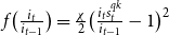 $f\big(\frac {i_t}{i_{t-1}}\big) = \frac {\chi }{2}\big(\frac {i_t s^{qk}_{t}}{i_{t-1}} -1\big)^2$
. Moreover,
 $\chi \gt 0$
reflects the magnitude of the adjustment cost, and
 $s_{t}^{qk}$
is the total factor productivity of the investment
 $i_t$
that follows an AR(1) process:
 \begin{align} \ln \left(s_{t}^{qk}\right) = \psi _{s^{qk}}\ln \left(s_{t-1}^{qk}\right)+ \varepsilon _{t}^{qk} \end{align}
where
 $\psi _{s^{qk}}$
measures the degree of persistence of
 $s_{t}^{qk}$
and
 $\varepsilon _{t}^{qk}$
is an investment-productivity shock with variance
 $\sigma ^{2}_{s^{qk}}$
. The capital producers’ optimization problem can be written as:
 \begin{align} \begin{aligned} \max _{\{i_t,k_t\}} \quad & \mathbb{E}_t \sum _{s=0}^{\infty } \Lambda _{t,t+s} \left [ q_t k_t - q_t(1-\delta ) k_{t-1} - i_t - \dfrac {\chi }{2} \left ( \dfrac {i_t s_{t}^{qk} }{i_{t-1}}-1\right )^2 i_t\right ] \\ \textrm {s.t.}\quad & k_t = (1-\delta )k_{t-1} + i_t \end{aligned} \end{align}
where
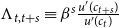 $\Lambda _{t,t+s} \equiv \beta ^s \frac {u'(c_{t+s})}{u'(c_t)}$
is the stochastic discount factor since households own capital producers. The capital producers’ problem yields the following relation to the capital price
 $q_t$
, taking the first-order condition with respect to
 $i_t$
:
 \begin{align} q_t &= 1 + \frac {\chi }{2}\left (\frac {i_t s_t^{qk}}{i_{t-1}}-1\right )^2 + \chi \left (\frac {i_t s_t^{qk}}{i_{t-1}}-1\right )\left (\frac {i_t}{i_{t-1}}\right )s_t^{qk} \notag \\ &\quad - \chi \mathbb{E}_t \left [ \Lambda _{t,t+1}\left (\frac {i_{t+1}s_{t+1}^{qk}}{i_t}-1\right ) \left (\frac {i_{t+1}}{i_t}\right )^2 s_{t+1}^{qk} \right ] \end{align}
All profits
 $\Gamma _{t}^{CP}$
earned outside the steady state (
 $q \neq 1$
) by the capital producers’ sector are returned to households, where
 $\Gamma _{t}^{CP} = (q_t -1)i_t - \frac {\chi }{2}\left (\frac {i_t s_{t}^{qk}}{i_{t-1}}-1\right )^2 i_t$
.
3.4 Retailers
The retailers are assumed to be monopolistically competitive. They buy wholesale good
 $y^{w}_{t}(i)$
from entrepreneurs at wholesale price
 $p^{w}_{t}(i)$
and differentiate it without cost. Each retailer
 $i$
then sells its unique variety
 $y_t(i)$
at nominal price
 $p_t(i)$
, applying a markup
 $x_t(i) = \frac {p_t(i)}{p^{w}_{t}(i)}$
on the wholesale price. The output of the final consumption good
 $y_t$
is a constant elasticity of substitution (CES) composite of all the different varieties produced by the retailers (using the Dixit and Stiglitz (Reference Dixit and Stiglitz1977) framework):
 \begin{align} y_t = \left [ \int _{0}^{1} y_{t} (i)^{\frac {\epsilon -1}{\epsilon }} di\right ]^{\frac {\epsilon }{\epsilon -1}} \end{align}
where
 $\epsilon \gt 1$
is the elasticity of substitution across different varieties. Retailers’ prices are sticky and indexed to a combination of past and steady-state inflation. Then, retailers must choose
 $\{p_t(i)\}_{t=0}^{\infty }$
to maximize profits given by:
 \begin{align} \Gamma ^{R} &= \mathbb{E}_t \sum _{s=0}^{\infty } \Lambda _{t,t+s} \Big [p_t(i) y_t(i) - p_t^{w}(i) y_t(i) - \frac {\kappa _{\pi }}{2}\Big (\frac {p_t(i)}{p_{t-1}(i)} - \pi _{t-1}^{\iota _p} \overline {\pi }^{\,1-\iota _p}\Big )^2 p_t y_t \Big ] \end{align}
subject to a downward-sloping demand coming from consumers’ maximization of a consumption aggregator:
 \begin{align} y_t(i) = y_t \left ( \dfrac {p_t(i)}{p_t}\right )^{-\epsilon } \end{align}
where
 $\kappa _{\pi }$
is a quadratic adjustment cost for changing prices beyond the indexation rule. In symmetrical equilibrium,
 $p_t(i) = p_t$
, the first-order conditions imply the Phillips curve, given by:
 \begin{align} \frac {\epsilon }{x_t} - \kappa _{\pi }\big (\pi _t - \pi _{t-1}^{\iota _p} \overline {\pi }^{1-\iota _p}\big )\pi _t + \mathbb{E}_t\!\left [ \Lambda _{t,t+1} \kappa _{\pi } \big (\pi _{t+1} - \pi _t^{\iota _p} \overline {\pi }^{1-\iota _p}\big ) \pi _{t+1}^2 \frac {y_{t+1}}{y_t}\right ] &= \epsilon - 1 \end{align}
where
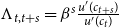 $\Lambda _{t,t+s} = \beta ^s \frac {u'(c_{t+s})} {u'(c_t)}$
is the stochastic discount factor since households own retail firms, and
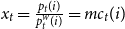 $x_t = \frac {p_t(i)}{p_{t}^{w}(i)} = mc_t(i)$
is the markup of the final good price.
3.5 Banks
The Cournot banking sector is used to characterize oligopolistic competition and capture banks’ market power, as the banking sector tends to be dominated by a few prominent players that accumulate capital.Footnote 10 The model’s framework does not allow new banks to enter the banking sector in response to profits, allowing the effects of Cournot competition to be analyzed without the dynamics of market entry. Stricter capital requirements can act as a barrier to entry for new banks, since these regulations require banks to maintain a considerable amount of capital, serving as a safety net that protects them from unexpected losses and ensures solvency during periods of financial stress. Thus, while stricter capital requirements promote financial stability, they may simultaneously deter new banks from entering the market.Footnote 11
Assume there are
 $N$
banks in the economy, indexed by
 $j$
. Banks have market power in conducting their intermediation activity, which allows them to adjust loan rates in response to adverse shocks. CBs play an essential role in the model, as they act as intermediaries for all financial transactions between agents in the economy and must satisfy the following balance-sheet identity:
 \begin{align} b_t(j) = d_t(j) + k^{B}_{t}(j) \end{align}
where loans
 $b$
equal deposits
 $d$
plus bank capital
 $k^{B}$
.Footnote
12
Equation (29) shows that banks use household deposits together with the capital accumulated over time to issue loans in the economy. However, the model does not consider factors that might discourage individuals from depositing their money in banks, such as low interest rates or lack of trust in the banking system. If such issues arose, banks would have to rely exclusively on liquidating their accumulated capital to provide loans, which could eventually lead to solvency problems.
Banks aim to keep the capital-to-loans ratio
 $\frac {k^B}{b}$
close to an optimal target
 $\tau ^{B}_{t}$
, which can be interpreted as a capital requirement imposed by the regulatory authority.Footnote
13
The capital requirement is essential for protecting banks from financial crises, ensuring that they have sufficient capital to meet deposit withdrawals and fulfill other obligations. Acting as an effective buffer, the capital requirement is a key element in the system’s resilience, absorbing financial shocks and enhancing stability.Footnote
14
The time-varying capital requirement ratio
 $\tau ^{B}_{t}$
will be the main instrument of macroprudential policy:
 \begin{align} \Omega _{t}^{B} (j) = \dfrac {\kappa _{k^B}}{2}\left (\dfrac {k^{B}_{t}(j)}{b_t(j)} - \tau ^{B}_{t} \right )^2 k^{B}_{t} (j) \end{align}
where
 $\kappa _{k^B}$
is the magnitude of the cost
 $\Omega ^{B}_{t}$
that banks incur if they deviate from
 $\tau ^{B}_{t}$
.Footnote
15
Thus, bank capital in period
 $t$
is accumulated from retained earnings
 $\Gamma ^{B}_{t}$
, after accounting for dividend payments
 $div_{t}^{B}$
, plus the bank capital
 $k_{t-1}^{B}$
from the previous period:
 \begin{align} k^{B}_{t} (j) = (1-\delta ^B)\dfrac {k^{B}_{t-1}(j)}{s^{k^B}_{t}} + \Gamma _{t}^{B}(j) - div^{B}_{t} (j) \end{align}
where
 $\delta ^B$
is the bank operation cost, and the retained earnings
 $\Gamma ^{B}_{t}$
can be written as:
 \begin{align} \Gamma _{t}^{B}(j) = \dfrac {1}{\pi _t}\left [ R_{t-1}^{b} \left (b_{t-1} (j) + \sum _{m \neq j} b_{t-1}(m) \right )b_{t-1}(j) - R_{t-1}^{d} d_{t-1}(j) - \Omega _{t-1}^{B}(j) \right ] \end{align}
The dependance of the loan rate
 $R^b$
on loans
 $b$
means that each bank
 $j$
has a certain degree of control over the equilibrium gross loan interest rate by adjusting its own quantity
 $b_t(j)$
given the amounts of
 $b_t(m)$
granted by the other banks (
 $m \neq j$
) in a banking system with a Cournot structure. Bank capital accumulation (31) is subject to an unexpected financial shock
 $s^{k^B}_{t}$
, which follows an AR(1):
 \begin{align} \ln \left(s^{k^B}_{t} \right) = \psi _{s^{k^B}} \ln \left(s^{k^B}_{t-1} \right) + \varepsilon ^{k^B}_{t} \end{align}
where
 $\varepsilon ^{k^B}_{t}$
is the financial shock with variance
 $\sigma ^{2}_{k^B}$
. In each bank’s optimization problem, bank
 $j$
maximizes the present discounted value of future dividends, subject to the bank capital accumulation law and
 $b(j), div(j) \geq 0$
:Footnote
16
 \begin{align} \max _{\{b_t(j), k^{B}_{t}(j), div_{t}^{B}(j)\}} \mathbb{E}_t \sum _{s=0}^{\infty } \Lambda _{t,t+s} \big[\ln \big(div_{t+s}^{B} (j)\big) \big] \end{align}
where
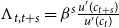 $\Lambda _{t,t+s} = \beta ^s\frac {u'(c_{t+s})}{u'(c_t)}$
is the stochastic discount factor, as households own the banks. Solving the banks’ optimization problem with respect to
 $b(j)$
, this yields:
 \begin{align} \mathbb{E}_t \Lambda _{t,t+1} \left \{\dfrac {\lambda _{t+1}^{B}(j)}{{\pi _{t+1}}} \left [ \dfrac {\partial \Omega _{t}^{B}(j)}{\partial b_t(j)} - \left (\dfrac {\partial R_{t}^{b}}{ \partial b_t(j)} b_t(j) + R_{t}^{b} - R_{t}^{d} \right ) \right ]\right \} = 0 \end{align}
where
 $\lambda _{t}^{B}(j)$
is the Lagrange multiplier of the banks’ optimization problem. In Cournot equilibrium, the total optimal loan quantity is
 $b_t = b_t(j) + \sum _{m\neq j} b_t(m)$
, and the total optimal bank capital is
 $k_{t}^{B} = k_{t}^{B}(j) + \sum _{m\neq j} k_{t}^{B}(m)$
. Assuming banks are identical,
 $b(j) = \frac {b_t}{N}$
,
 $k_{t}^{B}(j) = \frac {k_{t}^{B}}{N}$
, and
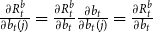 $\frac {\partial R_{t}^{b}}{\partial b_t(j)} = \frac {\partial R_{t}^{b}}{\partial b_t } \frac {\partial b_t}{\partial b_t(j)} = \frac {\partial R_{t}^{b}}{\partial b_t }$
. In Cournot equilibrium, the first-order condition (35) can be written as:
 \begin{align} \mathbb{E}_t \Lambda _{t,t+1} \left \{\dfrac {\lambda _{t+1}^{B}}{{\pi _{t+1}}} \left [ \dfrac {\partial \Omega _{t}^{B}}{\partial b_t} - \left (\dfrac {\partial R_{t}^{b}}{ \partial b_t} \dfrac {b_t}{N} + R_{t}^{b} - R_{t}^{d} \right ) \right ]\right \} = 0 \end{align}
The loan rate directly affects market loan demand
 $b_t$
because an increase in
 $R^{b}_{t}$
reduces entrepreneurs’ borrowing capacity. Furthermore, the loan rate has an indirect effect on loans taken by borrowers, influencing entrepreneurs’ demand for physical capital.Footnote
17
When bank
 $j$
chooses
 $b_t(j)$
to maximize dividends, it needs to consider how entrepreneurs would respond by changing their demand for physical capital,
 $\frac {\partial k_t}{\partial R_{t}^{b}}$
, which affects the level of investment in the economy. Entrepreneurs’ demand for physical capital decreases with the loan rate because
 $\frac {\partial k_t}{\partial R_{t}^{b}} \lt 0$
, and the interest rate elasticity of capital demand,
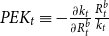 $PEK_t \equiv -\frac {\partial k_t}{\partial R_{t}^{b}}\frac {R^{b}_{t}}{k_t}$
, monotonically decreases with the expected marginal product of capital:
 \begin{align} PEK_t = \dfrac {1}{1-\alpha } \left ( \dfrac { m^{k}_{t}\mathbb{E}_t \left [ \dfrac {q_{t+1}(1-\delta )\pi _{t+1}}{R^{b}_{t}} \right ] }{ \mathbb{E}_t \left [\Lambda _{t,t+1}^{E} MPK_{t+1} \right ]} \right ) \end{align}
where
 $MPK_{t+1} \equiv \frac {\alpha z_{t+1} (k_t)^{\alpha -1} (l_{t+1})^{1-\alpha }}{x_{t+1}}$
is the marginal product of capital in real terms. The entrepreneurs’ loan demand elasticity
 $PED_t$
captures their dependency on the capital demand elasticity
 $PEK_t$
, which is given by:Footnote
18
 \begin{align} PED_t \equiv - \dfrac {\partial b_t} {\partial R_{t}^{b}} \dfrac {R_{t}^{b}}{b_t} = 1 + PEK \gt 0 \end{align}
Solving (36), the following expression for the loan interest rate is obtained, assuming
 $\Lambda _{t,t+1} \gt 0$
and
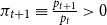 $\pi _{t+1} \equiv \frac {p_{t+1}}{p_t} \gt 0$
:
 \begin{align} R_{t}^{b} = \dfrac {R_{t}^{d} - \kappa _{k^B}\left (\dfrac {k_{t}^{B}} {b_{t}} - \tau ^{B}_{t} \right ) \left (\dfrac {k_{t}^{B}}{b_t} \right )^2}{\left (1 - PED_{t}^{-1} \dfrac {1}{N} \right )} \end{align}
where
 $N$
is the number of banks,
 $\kappa _{k^B}$
is the bank capital adjustment cost, and the spread, given by
 $R^b - R^d$
, is the difference between the rate charged on loans taken by entrepreneurs and the rate paid on households’ deposits.
From (39),
 $R_{t}^{b}$
decreases with the number of banks
 $N$
(more banking competition), and with the elasticity
 $PED_t$
. Entrepreneurs respond quickly to an increased loan interest rate and reduce the amount of loans
 $b_t$
demanded, which forces banks to lower
 $R_{t}^{b}$
. Modeling the leverage level of banks (and their capital accumulation) allows the introduction of shocks originating on the credit supply side. This framework enables the study of their effects on setting loan rates subject to capital requirements and their propagation in the real economy. In particular, it is possible to analyze the impact of a weakening in the balance sheet position of the Cournot banking sector, arising from an exogenous shock that destroys banking capital.
In an environment characterized by Cournot competition with bank capital adjustment cost
 $\kappa _{k^B}$
, if banks maintain a
 $\frac {k^B}{b}$
ratio above the minimum requirement imposed by the macroprudential authority, the excess capital would have several implications for the equilibrium loan rate
 $R^b$
. Specifically, higher capital ratios could lead to a situation where the interest rate on deposits exceeds the interest rate on loans. This misalignment would result in significant financial losses for banks, as they pay higher rates to depositors while receiving lower rates on loans. Consequently, banks would have no incentive to accumulate capital beyond what the macroprudential authority mandates.
3.6 Equilibrium
Equilibrium is imposed on the deposit and loan markets, and the aggregate resource constraint is:
 \begin{align} c_t + c^{E}_{t} + i_t + div_{t}^{B} + \dfrac {\kappa _{\pi }}{2} (\pi _t - \overline {\pi })^2 y_t + \frac {\chi }{2}\left (\frac {i_t}{i_{t-1}}-1\right )^2 i_t + \dfrac {\kappa _{k^B}}{2}\left (\frac {k_{t}^{B}}{b_{t}} - \tau ^{B}_{t} \right )^2 k_{t}^{B} = y_t \end{align}
The new capital supplied by capital producers equals entrepreneurs’ capital demand, and the labor supplied by households equals entrepreneurs’ labor demand. The Cournot equilibrium of the banking sector can be written as:
 \begin{align} b_t^{B} = \sum _{j=1}^{N} b_t(j), \quad d_t^{B} = \sum _{j=1}^{N} d_t(j), \quad k_t^{B} = \sum _{j=1}^{N} k_t^{B}(j) \end{align}
where the banking sector’s loan supply
 $b^{B}_{t}$
equals market loan demand
 $b_{t}$
; the banking sector’s demand for deposits
 $d^{B}_{t}$
equals households’ deposit supply
 $d_{t}$
; and the banking system capital
 $k_{t}^{B}$
is equal to the sum of the
 $N$
banks’ capital. From (29), the total loan supply
 $b_{t}^{B}$
equals the total deposits
 $d^{B}_{t}$
held in the banking system plus the total capital accumulated
 $k_{t}^{B}$
in the banking sector:
 \begin{eqnarray} b_{t}^{B} = d^{B}_{t} + k_{t}^{B} \end{eqnarray}
4. Policy regimes
Two types of policy interventions can be considered. First, monetary policy has real effects due to sticky prices. Second, the macroprudential authority is assumed to affect the spread by imposing additional capital requirements or provisions when credit growth is above its steady-state value. In the model, monetary policy is kept fixed over time. The effects of introducing macroprudential policy are analyzed in an environment of IBC, where banks can accumulate capital subject to adequacy costs and time-varying capital requirements.
4.1 Monetary policy
The central bank instrument is modeled using the Taylor rule, specified as:
 \begin{align} R_{t} = (1-\rho _r)\overline {R} + (1-\rho _r) [\phi _{\pi }(\pi _t - \overline {\pi }) + \phi _{y}(y_t - \overline {y})] + \rho _r R_{t-1} \end{align}
where
 $\phi _{\pi }$
and
 $\phi _{y}$
measure the responses to inflation and output deviations from their targets, and
 $\rho _r$
captures the persistence in interest rate adjustments. In this economy, the central bank controls the gross nominal interest rate on deposits
 $R^{d}$
paid by CBs to households, according to the Taylor rule. In this way,
 $R^{d}_{t} = R_t$
, and deviations in inflation and output from their respective targets affect the deposit rate
 $R^d$
.
4.2 Macroprudential policy
In line with Angelini et al. (Reference Angelini, Neri and Panetta2014), it is assumed that macroprudential authorities react to abnormal credit behavior, as one of the objectives of macroprudential policy is to ensure the financial system’s resilience. Time-varying capital requirements are chosen as the macroprudential instrument for two main reasons. First, banking capital has been central in the debate on regulatory reform, and the Basel III package has recently introduced a countercyclical capital requirement. Second, systemic financial crises directly or indirectly affect banking capital and credit supply. Thus, the model directly addresses how capital buffers influence the banking sector’s ability to withstand shocks and continue lending. The macroprudential authority is assumed to define a time-varying capital requirement rule, as follows:
 \begin{align} \tau ^{B}_{t} = (1-\rho _{\tau ^B})\overline {\tau }^B + (1-\rho _{\tau ^B}) \left [ \chi _{\tau ^B} \left ( \dfrac {b_t}{y_t} - \dfrac {\overline {b}}{\overline {y}} \right )\right ] + \rho _{\tau ^B} \tau ^{B}_{t-1} \end{align}
where
 $\overline {\tau }^B$
is the steady-state value of
 $\tau ^{B}_{t}$
. In the baseline specification of (44), the macroprudential authority is assumed to adjust capital requirements only in response to deviations in the loans-to-output ratio.Footnote
19
The parameter
 $\chi _{\tau ^B}$
in macroprudential policy measures the response of capital requirements to deviations of the loans-to-output ratio from its target
 $\frac {\overline {b}}{\overline {y}}$
. This parameter captures how aggressively the macroprudential authority reacts to discrepancies between the actual loan-to-output ratio and its target. If
 $\chi _{\tau ^B} \gt 0$
, an increase in
 $\frac {b}{y}$
above its target causes the macroprudential authority to raise capital requirements
 $\tau ^B$
, making policy countercyclical. If
 $\chi _{\tau ^B} \lt 0$
, policy is procyclical, and an increase in
 $\frac {b}{y}$
above its target reduces capital requirements. If
 $\chi _{\tau ^B} = 0$
, no macroprudential policy is applied. As the macroprudential instrument affects lending rates, policymakers can directly offset fluctuations in the spread caused by adverse shocks.
5. Calibration and bayesian estimation
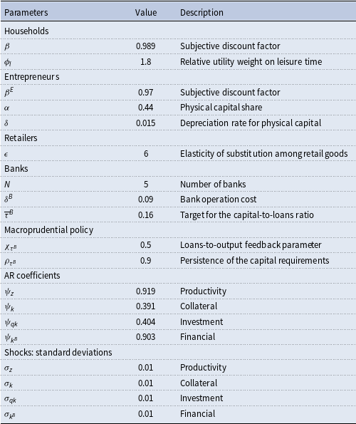
The structural parameters of the model are divided into calibrated and estimated parameters. The calibrated parameters are chosen to match the Brazilian economy. Parameters for which Brazilian data are not available are calibrated following the strategy of Gerali et al. (Reference Gerali, Neri, Sessa and Signoretti2010), Angelini et al. (Reference Angelini, Neri and Panetta2014), and Li (Reference Li2021). The calibration information is summarized in Table 1. Subjective discount factors are set to
 $0.989$
for saving households and
 $0.97$
for borrowing entrepreneurs, following De Castro et al. (Reference De Castro, Gouvea, Minella, Santos and Souza-Sobrinho2015) and Gerali et al. (Reference Gerali, Neri, Sessa and Signoretti2010). The relative utility weight of leisure time,
 $\phi _l$
, in the households’ utility function is
 $1.8$
, in line with Li (Reference Li2021) and Gerali et al. (Reference Gerali, Neri, Sessa and Signoretti2010). In the retailers’ market, the elasticity of substitution among retail goods,
 $\epsilon$
, is set to 6, generating a 20% markup of the final good price
 $\big(x=\frac {\epsilon }{\epsilon -1}\big)$
in the steady state, a value commonly used in the literature.
Calibrated parameters

In the production sector, the depreciation rate,
 $\delta$
, for physical capital is set to 0.015, and the capital share,
 $\alpha$
, is 0.44, following De Castro et al. (Reference De Castro, Gouvea, Minella, Santos and Souza-Sobrinho2015). The number of banks,
 $N$
, is set to 5 to represent the five largest Brazilian banks. The bank operation cost,
 $\delta ^B$
, is 0.09, and the optimal leverage target,
 $\tau ^B$
, is 0.16 (in the absence of macroprudential policy), following Ferreira et al., (Reference Ferreira and Nakane2015).
The persistence parameter of macroprudential policy,
 $\rho _{\tau ^B}$
, is set to 0.9, and the feedback parameter on the loans-to-output ratio,
 $\chi _{\tau ^B}$
, is set to 0.5, following Angelini et al. (Reference Angelini, Neri and Panetta2014). The positive coefficient of
 $\chi _{\tau ^B}$
indicates that macroprudential policy is countercyclical: capital requirements increase when credit expands in the economy. Brazilian values are used for the shocks’ persistence parameters, following Melo (Reference Melo2022). Four adverse shocks are considered: productivity, collateral, financial, and investment. The smallest standard deviations for the shocks are used, in line with Angelini et al. (Reference Angelini, Neri and Panetta2014), to assess the impact of macroprudential policy on agents’ welfare and the fluctuations of the main model variables.
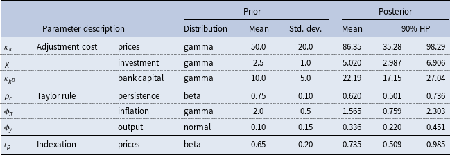
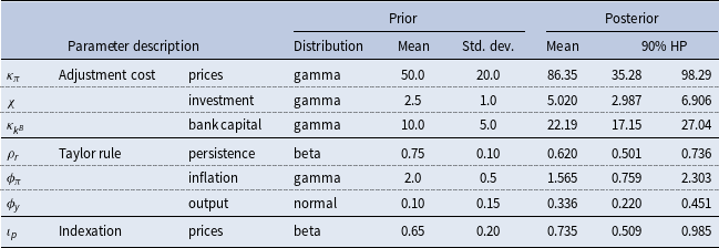
The other parameters were estimated in Melo (Reference Melo2022) using quarterly time series of six Brazilian variables from 2000-Q3 to 2019-Q4. The variables considered are GDP, investment, IPCA inflation, the official inflation index adopted in Brazil, the nominal short-term interest rate (Selic), loans to firms (working capital), and deposits. The estimated values are provided in Table 2. The investment adjustment cost,
 $\chi$
, for Brazil is 5.02. The prices adjustment cost,
 $\kappa _{\pi }$
, is 86.35, and the prices indexation parameter,
 $\iota _p$
, is set to 0.73 in the Phillips curve. I estimated a value of 22.19 for the bank capital adjustment cost,
 $\kappa _{k^B}$
, for Brazilian banks. Regarding the monetary policy parameters, the inflation and output response parameters are estimated as
 $\phi _{\pi } = 1.56$
and
 $\phi _{y} = 0.33$
, respectively, and the monetary policy persistence parameter is estimated as
 $\rho _r = 0.62$
.
Prior and posterior distribution of structural parameters
6. Interaction between monetary and macroprudential policies
In this section, I analyze the effects of adverse shocks on the model’s macroeconomic variables. Two scenarios are considered. The first is a baseline scenario (TR) with only monetary policy, modeled using the standard form of a Taylor rule. The second is an alternative scenario (MP) in which macroprudential policy is active. I also assess the importance of macroprudential policy in mitigating spread fluctuations and, consequently, reducing the impact on accumulated output and other macroeconomic variables.
6.1 Productivity shock
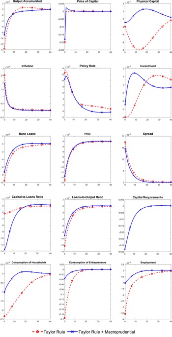
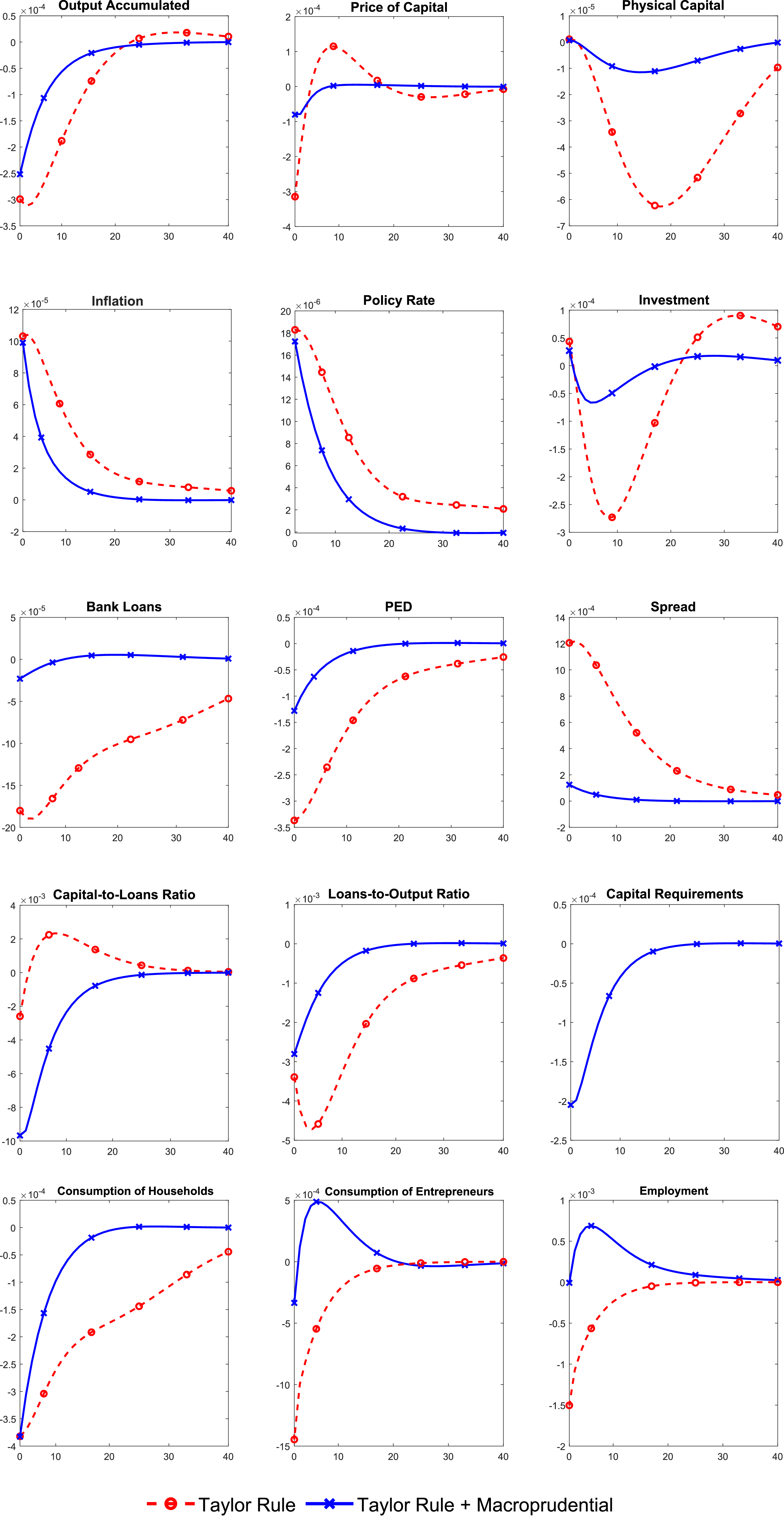
Figure 1 shows the impulse responses to an adverse productivity shock
 $z$
for loans, inflation, the spread, and other main variables. The scenario with only monetary policy amplifies the negative shock
 $z$
’s effects on output
 $y$
in the initial quarters. Productivity
 $z$
falls at the beginning of period one, reducing the expected Marginal Product of Capital (MPK). The decline in MPK lowers entrepreneurs’ demand for physical capital and causes a drop in its price
 $q$
. The reduction in entrepreneurs’ collateral value makes them more financially constrained with inelastic demand for loans. Under Cournot competition, banks respond to the more inelastic loan demand by reducing their loan supply to achieve a higher loan rate, which leads to a rise in the spread.
A higher spread allows banks to accumulate more capital, increasing the
 $\frac {k^B}{b}$
ratio in both policy scenarios. However, the reduction in loans provided by banks leads to a fall in the loans-to-output ratio, triggering a response from the macroprudential authority, which reduces the capital requirement
 $\tau ^{B}$
. The movement of
 $\tau ^{B}$
in the opposite direction of the
 $\frac {k^B}{b}$
ratio mitigates the effect of the productivity shock through the BS channel. Consequently, the spread increase is more significant when only monetary policy is active, compared to the scenario with active macroprudential policy.
The differential responses of output and other macroeconomic variables under the two policy scenarios can be explained by the difference in spread fluctuations when capital requirements vary over time. The lower cost of loans under active macroprudential policy impacts entrepreneurs’ accumulation of physical capital
 $k$
and the level of investments. The decline in
 $k$
is larger in the scenario with only monetary policy. Entrepreneurs’ capital begins to recover around 20 quarters after the initial shock in the scenario with macroprudential policy. This coincides with the period when the spread returns to its initial equilibrium and fluctuations are eliminated. The fall in output
 $y$
under active macroprudential policy is smaller than in the scenario with only monetary policy.
Given that entrepreneurs use bank loans
 $b$
to finance their activities, reducing the cost of loans in the presence of macroprudential policy allows them to face a smoother budget constraint, thereby raising their consumption level
 $c^{E}$
compared to the scenario with only monetary policy. A similar pattern is observed for household consumption
 $c$
, where the smaller decline in accumulated output
 $y$
under macroprudential policy results in higher household income and, consequently, higher consumption. With a smaller drop in
 $y$
and other productive sectors being less affected, the decline in labor
 $l$
hired by entrepreneurs is also smaller compared to the scenario with only monetary policy, with employment returning to its initial equilibrium after about 20 quarters following the negative productivity shock. Figure 1 shows that the larger decline in accumulated output in the only monetary policy scenario leads to higher inflation, which reduces households’ purchasing power. In this way, the central bank increases the policy rate to restore households’ consumption.
Impulse responses to a negative productivity shock.
Note: IRFs to a negative
 $z$
shock under the baseline (TR) and time-varying capital requirements (MP) scenarios.

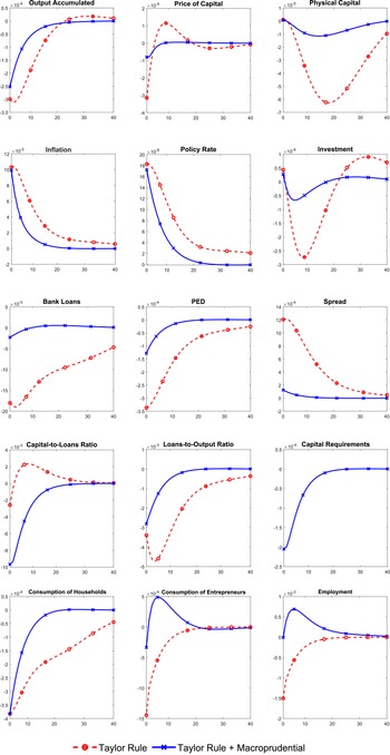
Impulse responses to a negative collateral shock.
Note: IRFs to a negative
 $m^k$
shock under the baseline (TR) and time-varying capital requirements (MP) scenarios.
6.2 Collateral shock
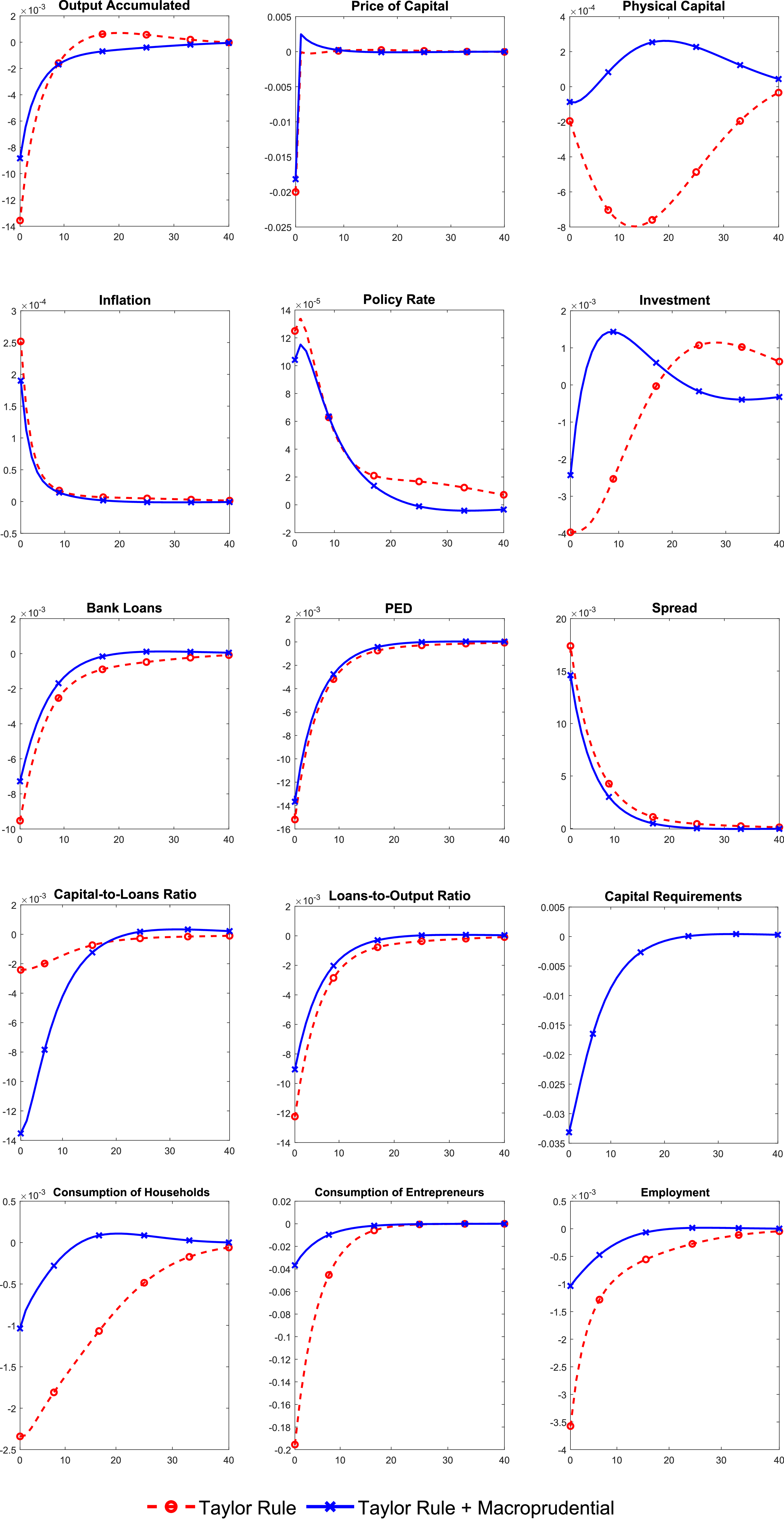
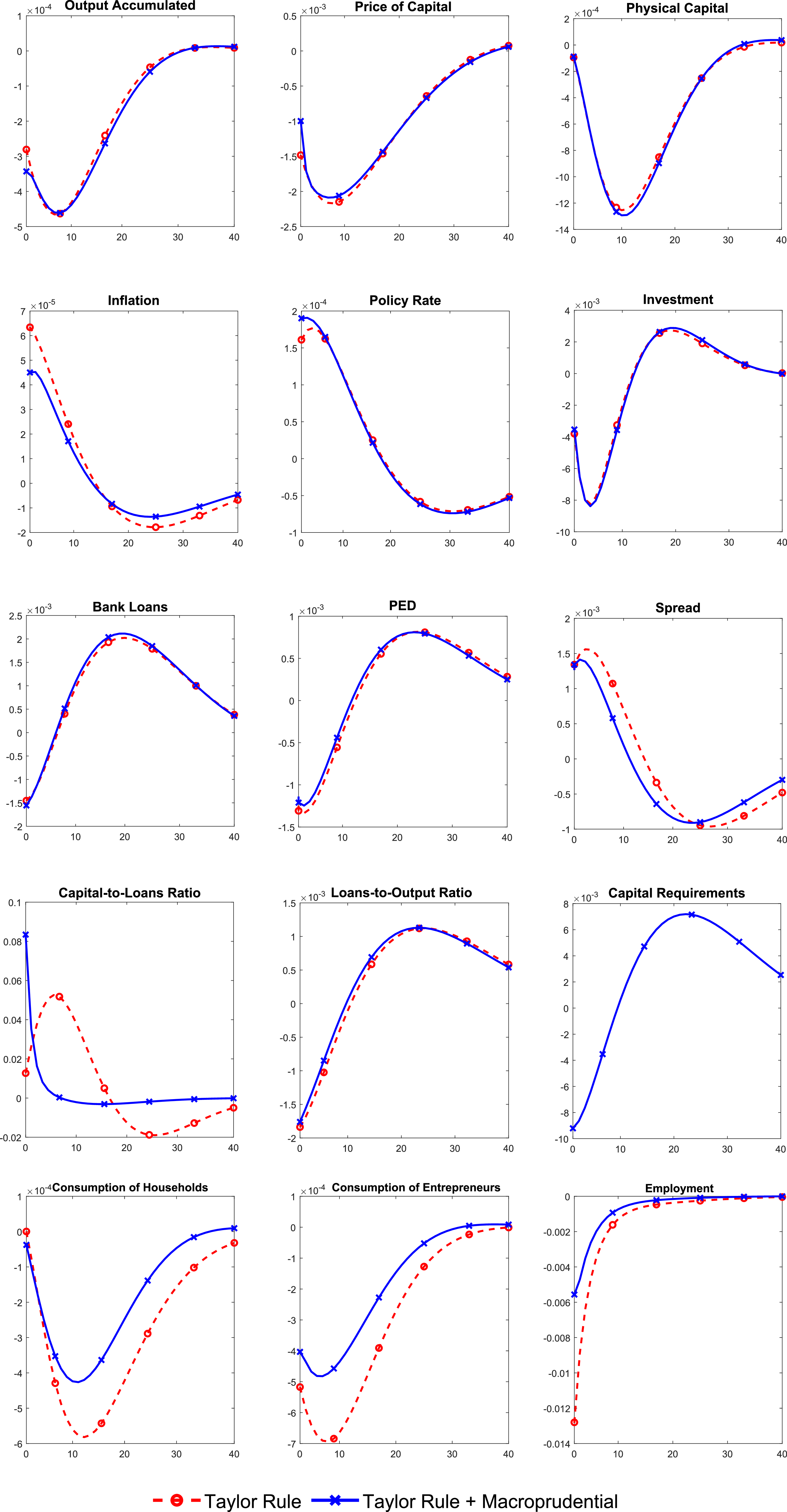
Figure 2 shows the effects of a negative collateral shock
 $m^k$
that reduces the guarantees entrepreneurs can pledge as collateral to obtain loans.Footnote
20
This adverse shock affects entrepreneurs’ loan demand elasticity (PED), making them more financially constrained. Banks respond by reducing loan supply to raise the loan rate, given the more inelastic demand and entrepreneurs’ reliance on credit. However, even if banks set a higher loan rate, the reduction in entrepreneurs’ collateral prevents an increase in bank capital accumulation
 $k^B$
, which directly lowers the capital-to-loans ratio. The decline in
 $\frac {k^B}{b}$
generates a higher amplification of the spread if capital requirements
 $\tau ^B$
were fixed over time. Under Cournot competition and time-varying capital requirements, banks adjust by reducing the loans-to-output ratio
 $\frac {b}{y}$
. In response, the macroprudential authority lowers capital requirements, according to (44). This policy intervention mitigates the amplification of the spread through the bank-stress channel, leading to a more favorable economic outcome under active macroprudential policy.
Investment recovers rapidly when macroprudential policy is active, taking about five quarters to return to its initial equilibrium. With only monetary policy, a return to the initial equilibrium occurs about 20 quarters after the shock. The rapid recovery of entrepreneurs allows physical capital
 $k$
to return to its initial equilibrium within a few periods under active macroprudential policy. In contrast, the fall in physical capital lasts around 15 quarters with only monetary policy, and full recovery is achieved only after 40 quarters. Therefore, the quick recovery of investment by entrepreneurs affects accumulated output in the economy, preventing a decline in output as severe as in the scenario with only monetary policy. Thus, the output decline under active macroprudential policy is smaller than in the scenario with only monetary policy.
Figure 2 also shows that the agents most affected by a negative collateral shock are entrepreneurs, who experience a sharp decline in consumption following the reduction in credit granted by oligopolistic banks due to the loss of part of their collateral. With only monetary policy, entrepreneurs’ consumption
 $c^E$
takes around 20 quarters to return to its initial equilibrium, whereas the introduction of macroprudential policy reduces this time to approximately 10 quarters, due to the lower cost of credit. The decline in entrepreneurs’ assets caused by the negative collateral shock also affects labor, resulting in a sharp drop when there is no regulation on CBs. Employment recovery takes approximately 40 quarters. For this negative shock, the central bank responds to the increase in inflation by raising the policy rate.
6.3 Financial shock
Figure 3 shows the effects of a bank capital loss resulting from an unexpected shock that destroys bank capital
 $k^B$
. It can be observed that macroprudential policy is more effective in reducing the spread amplification for this type of shock because it acts through the BS channel. A sudden drop in bank capital (31) reduces the capital-to-loans ratio
 $\frac {k^B}{b}$
and increases the loan rate in (39). The increase in the loan rate
 $R^b$
is a mechanism that banks use to recover their losses in the oligopolistic banking sector, which directly raises the spread. In the model,
 $\chi _{\tau ^B} = 0.5$
ensures that
 $\tau ^B$
reacts countercyclically to the loans-to-output ratio and remains highly persistent (
 $\rho _{\tau ^B} = 0.9$
).
Impulse responses to a negative financial shock.
Note: IRFs to a negative
 $s^{k^B}$
shock under the baseline (TR) and time-varying capital requirements (MP) scenarios.
Impulse responses to a negative investment shock.
Note: IRFs to a negative
 $s^{qk}$
shock under the baseline (TR) and time-varying capital requirements (MP) scenarios.
Comparing both policy scenarios reveals that monetary policy alone is insufficient to stabilize the economy under an adverse financial shock. When time-varying capital requirements are implemented, spread fluctuations are significantly lower. The reduction in the loans-to-output ratio
 $\frac {b}{y}$
due to the decline in loans, triggers an adjustment in capital requirements (44), lowering them. This reduces the gap between the capital-to-loans ratio
 $\frac {k^B}{b}$
and the capital requirements
 $\tau ^B$
. With the smaller increase in the spread, entrepreneurs are less financially constrained, mitigating the fall in investment when macroprudential policy is active. The lower cost of credit also reduces the decline in physical capital
 $k$
compared to the scenario with only monetary policy. Consequently, the mitigated effect on the spread results in a smaller contraction of accumulated output.
The implementation of a macroprudential policy to minimize the effects of a negative financial shock directly impacts entrepreneurs’ consumption, causing
 $c^E$
to rapidly recover to equilibrium due to the lower cost of bank credit. Consequently, entrepreneurs can maintain higher leverage, and their consumption returns to equilibrium after roughly 25 quarters. A similar pattern is observed for employment, which returns to its initial equilibrium within 20 quarters as investment by entrepreneurs recovers in the presence of macroprudential policy.
However, households experience a sharp drop in consumption
 $c$
in the absence of macroprudential policy, as they receive lower dividends from oligopolistic banks that incur costs due to deviation from the optimal target
 $\tau ^B$
. Additionally, households face reduced hiring opportunities from entrepreneurs and lower profits from the capital-producing and retail sectors, given the decline in productive activity. Figure 3 shows that in an adverse financial shock scenario, the central bank responds to the smaller increase in inflation under active macroprudential policy with a correspondingly lower increase in the policy rate, compared to the scenario with only monetary policy.
6.4 Investment shock
Figure 4 shows the effects of a negative investment shock, which increases the cost of transforming old physical capital into new capital for the production of wholesale goods. This shock explicitly affects capital producers in the economy. The investment shock reduces the price
 $q$
of collateral that entrepreneurs can offer to banks to obtain loans, making them more financially constrained (inelastic PED). However, the impact of the investment shock on the spread is not mitigated by macroprudential policy at time zero; the spread trajectories start to diverge only after a few quarters. It can be observed that, following a negative investment shock, the spread returns to its initial equilibrium after approximately 40 quarters, regardless of whether macroprudential policy is active. Figure 4 also shows that macroprudential policy is not more effective than monetary policy in reducing fluctuations in output, investment, or physical capital.
The banks’ decision to reduce loans
 $b$
and consequently increase the spread leads to a fall in the loans-to-output ratio
 $\frac {b}{y}$
, which in turn reduces capital requirements set by the macroprudential authority. After a negative investment shock, the capital-to-loans ratio
 $\frac {k^B}{b}$
increases significantly, indicating a rapid recovery of bank capital. This immediate response reflects the market power of the Cournot banking system. Opposite movements in
 $\frac {k^B}{b}$
and
 $\tau ^B$
reduce the spread amplifying effect after a few periods following the initial shock when macroprudential policy is active. Approximately 10 quarters after the shock, the initial recovery of investment and physical capital begins to influence accumulated output, with
 $y$
returning to its initial level roughly 30 quarters after the investment shock in both policy scenarios.
Negative investment shock also has a negative impact on the productive activity of entrepreneurs, who face higher production costs and consequently begin to hire fewer workers. Regarding employment, it is noticeable that in the absence of macroprudential policy, the decline becomes more pronounced due to the elevated cost of credit, which slows down entrepreneurs’ capacity to invest and hire new labor. It can be observed that the recovery of employment occurs approximately 30 quarters after the shock. The reduction in productive activity also makes it more difficult for entrepreneurs to sell their old capital at price
 $q$
and to sell the wholesale good
 $y^w$
to retailers, thereby reducing their consumption
 $c^E$
.
Figure 4 shows that the return of
 $c^E$
to its initial equilibrium in the scenario with macroprudential policy occurs almost simultaneously with the return in the scenario with only monetary policy. However, the negative investment shock does not affect households’ consumption
 $c$
immediately, and after about 10 quarters, household consumption recovers more quickly in the presence of macroprudential policy. With only monetary policy, household consumption takes more than 40 quarters to return to its initial equilibrium, whereas with active macroprudential policy, recovery occurs in roughly 30 quarters.
7. Welfare analysis
This section focuses on evaluating whether the introduction of macroprudential policy can improve the welfare of economic agents given an established monetary policy, using a second-order approximation of the equilibrium. A grid is constructed over which the macroprudential policy can vary. To assess the efficiency of different policies, welfare is numerically compared across two scenarios. The first is the baseline scenario (TR) with only monetary policy, implemented via the standard Taylor rule. The second is an alternative scenario (MP) with both monetary and macroprudential policies.
Monetary policy is kept fixed over time.Footnote 21 This study examines whether the introduction of countercyclical macroprudential policy improves agents’ welfare following four adverse shocks in an economy with a Cournot banking system: (i) productivity, (ii) collateral, (iii) financial, and (iv) investment. The economy comprises three main agents: households, entrepreneurs, and banks. The analysis also considers the effects of increasing the macroprudential policy response to the loans-to-output ratio and heightened banking competition.
Welfare is measured as the unconditional expectation of the average utility of households, entrepreneurs, and banks. Accordingly, welfare is evaluated separately for households,
 $W^{H}_{t}$
, entrepreneurs,
 $W^{E}_{t}$
, and banks,
 $W^{B}_{t}$
, following the equations:Footnote
22
 \begin{align} W_t^{H} &\equiv \mathbb{E}_t \sum _{s=0}^{\infty } \beta ^s \big [\ln (c_{t+s}) + \phi _l \ln (1-l_{t+s})\big ] \\[-14pt] \nonumber \end{align}
 \begin{align} W_t^{E} &\equiv \mathbb{E}_t \sum _{s=0}^{\infty } (\beta ^{E})^{s} \big [\ln \left(c_{t+s}^{E} \right)\big ] \\[-14pt] \nonumber \end{align}
 \begin{align} W_t^{B} &\equiv \mathbb{E}_t \sum _{s=0}^{\infty } \beta ^{s} \big [\ln \left(div^{B}_{t+s} \right)\big ] \\[12pt] \nonumber \end{align}
where
 $\mathbb{E}$
denotes the unconditional expectation operator. The policy rules in the model are designed to be both implementable and simple, as they are functions of observable macroeconomic indicators.Footnote
23
In the model, macroprudential policy is simple because it depends on observable macroeconomic variables (output
 $y$
and loans
 $b$
), and implementable because the policy coefficients
 $(\rho _{\tau ^B}, \chi _{\tau ^B})$
are restricted to an interval that guarantees a unique, bounded, approximate second-order solution.
According to Ferreira et al., (Reference Ferreira and Nakane2015), there is greater uncertainty regarding the macroprudential policy parameter; therefore, I restrict the reaction of capital requirements to the loans-to-output ratio to the range
 $\chi _{\tau ^B} \in [0,5]$
, which is narrower than the range used by other authors, who vary
 $\chi _{\tau ^B}$
between
 $0$
and
 $10$
. My range for
 $\chi _{\tau ^B}$
is partitioned using grids of size 0.1. Following Angelini et al. (Reference Angelini, Neri and Panetta2014), I assume that
 $\chi _{\tau ^B} = 0$
implies the absence of macroprudential policy. In the baseline analysis, I consider
 $\chi _{\tau ^B} = 0.5$
for the macroprudential policy. I also examine how an increase in banking competition can improve welfare by varying the number of banks
 $N$
within the range
 $[5,30]$
.
I present welfare gains in terms of consumption equivalents. I assess welfare when only monetary policy is active and compare it with welfare under the joint implementation of monetary and macroprudential policies. The objective is to quantify the welfare benefits of introducing a macroprudential policy. The consumption equivalent is an intuitive measure that allows us to evaluate the gains (or losses) from macroprudential policy and defines the maximum fraction of consumption
 $\lambda$
that agents would be willing to forgo in an economy with only monetary policy (TR) to enter an economy where macroprudential policy is active (MP).Footnote
24
Formally,
 $\lambda$
must satisfy the following conditions for households
 $(H)$
, entrepreneurs
 $(E)$
, and banks
 $(B)$
, respectively:
 \begin{align} \lambda ^{H} &= \exp \!\big [(1-\beta ) \big(W^{H,MP} - W^{H,TR} \big)\big ] - 1 \\[-12pt] \nonumber \end{align}
 \begin{align} \lambda ^{E} &= \exp \!\big [(1-\beta ^{E}) \big(W^{E,MP} - W^{E,TR}\big)\big ] - 1 \\[-12pt] \nonumber \end{align}
 \begin{align} \lambda ^{B} &= \exp \!\big [(1-\beta )\big(W^{B,MP} - W^{B,TR}\big)\big ] - 1 \\[12pt] \nonumber \end{align}
where
 $W^{i, MP}$
,
 $i = \{H, E, B\}$
, denotes the welfare of agents when the macroprudential policy is active, and
 $W^{i, TR}$
represents the welfare obtained in the absence of macroprudential policy.Footnote
25
7.1 Negative productivity shock
Table 3 presents the welfare gains of households, entrepreneurs, and oligopolistic banks resulting from the introduction of macroprudential policy, while keeping the baseline calibration for policy parameters, in the event of a negative productivity shock. Entrepreneurs benefit from time-varying capital requirements as a macroprudential instrument, mainly due to the lower cost of credit. As the economy’s borrowers, entrepreneurs are affected by the BS channel when adverse shocks cause fluctuations in the capital-to-loans ratio and increase the loan rate, even when these shocks originate in the IBC channel. In this context, a reduction in capital requirements narrows the gap
 $\big(\frac {k^B}{b} - \tau _{t}^{B}\big)$
, which otherwise elevates the loan rate after an adverse productivity shock. This lowers credit costs and helps guide the economy toward a low-inflation, high-output equilibrium relative to a scenario with only monetary policy, as illustrated in Figure 1.
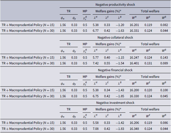
Welfare gains with baseline parameters – negative productivity shock

 $^*$
Welfare gains compared with the baseline policy regime (only TR).
Welfare gains with
 $\chi _{\tau ^B} \in [0,5]$
– negative productivity shock.
Note: Welfare gains from introducing the macroprudential regulation, given monetary policy (different values of the loans-to-output feedback parameter in the time-varying capital requirement rule).
Entrepreneurs can leverage their investment with a lower cost of credit, which directly increases the level of accumulated output
 $y$
in the economy and, consequently, their consumption
 $c^E$
and welfare
 $W^E$
with a gain of 0.22%. Moreover, macroprudential policy can enhance the welfare of households, as the growth in accumulated output resulting from higher investment activity by entrepreneurs tends to bring the economy to an equilibrium with higher aggregate consumption and lower inflation. This positively affects households’ real earnings, allowing them to smooth their consumption over time. In contrast, macroprudential policy reduces the welfare gains of banks. The amplification effect of the productivity shock is smaller because the BS channel has less impact on the increase of the loan rate. With a lower loan rate
 $R^b$
and a smaller spread, oligopolistic banks accumulate less capital
 $k^B$
and consequently pay lower dividends
 $div^B$
. Table 3 shows that, under the baseline calibration, macroprudential policy results in a -0.40% change in banks’ welfare gains.
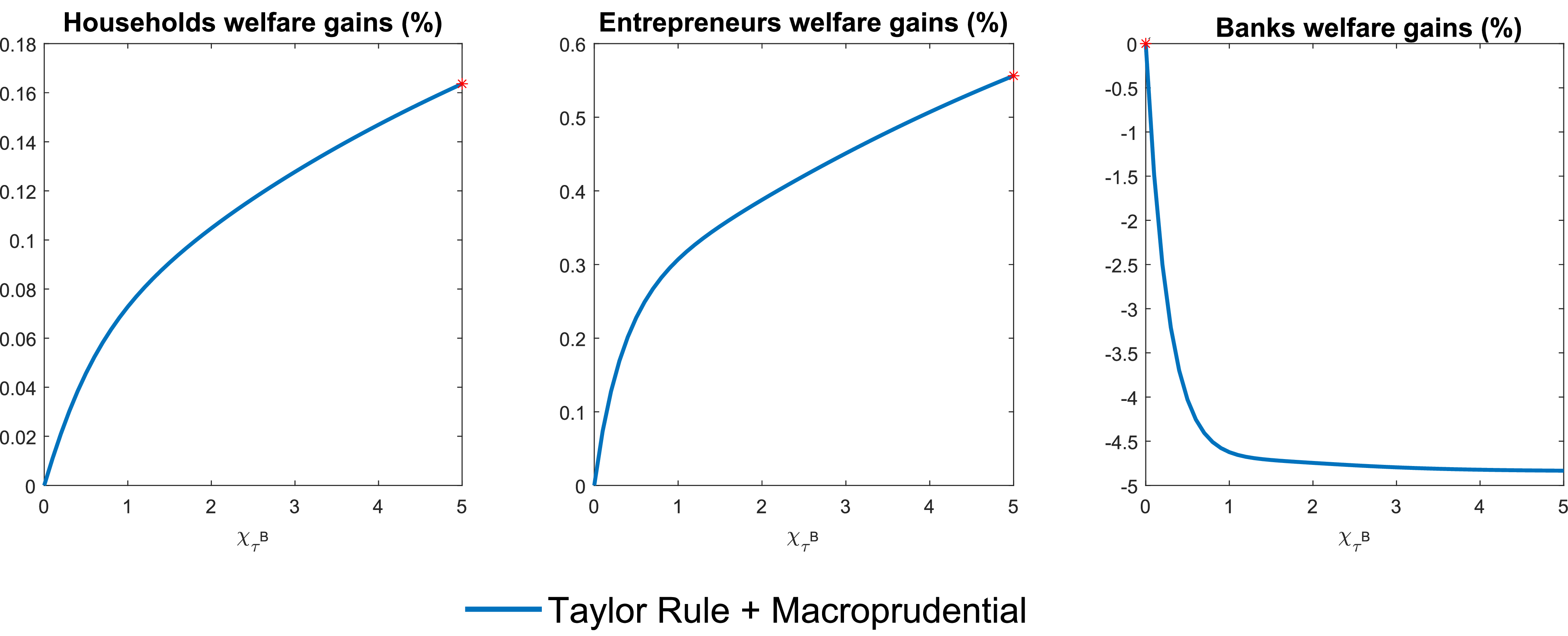
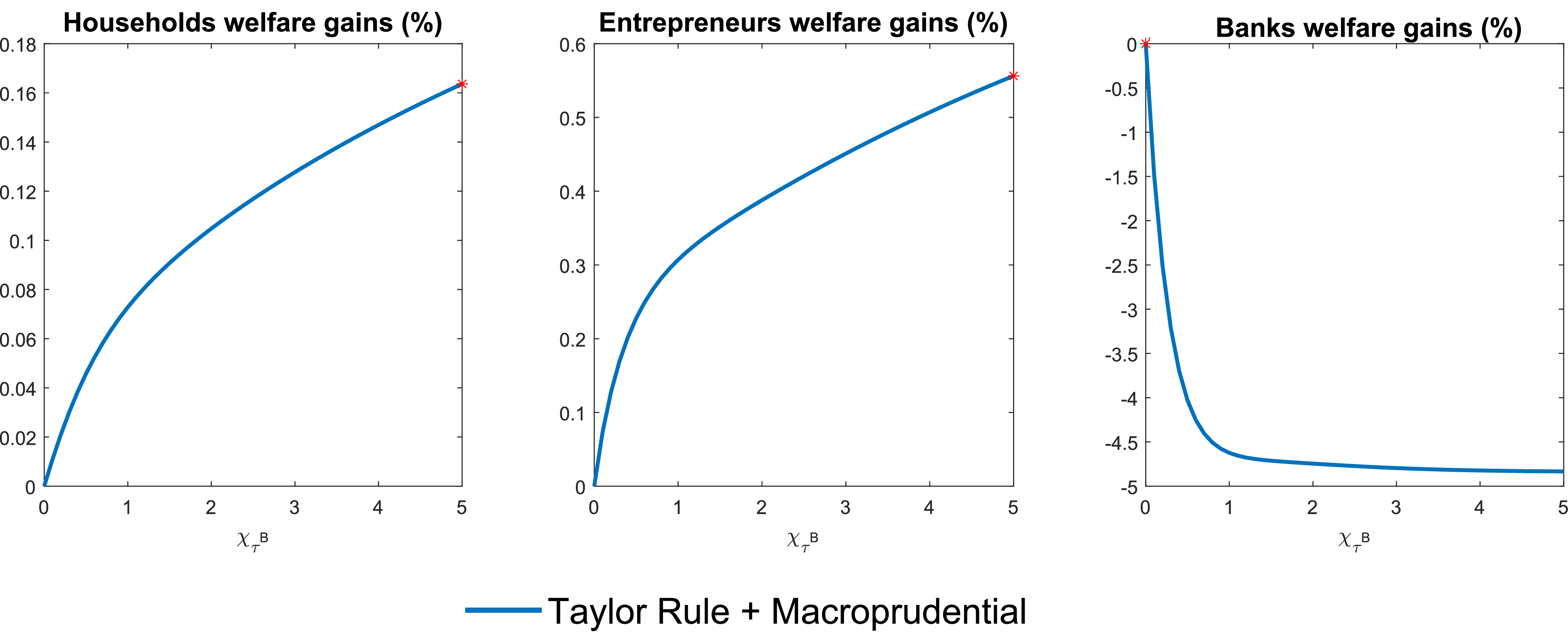
Figure 5 shows the scenario in which macroprudential policy is active and
 $\chi _{\tau ^B}$
varies in the interval
 $[0,5]$
. If
 $\chi _{\tau ^B} = 0$
, there is no macroprudential policy. The monetary policy parameters are set to their baseline values:
 $\phi _{\pi } = 1.56$
and
 $\phi _{y} = 0.33$
. Higher values of
 $\chi _{\tau ^B}$
correspond to larger welfare gains for households and entrepreneurs, and to welfare losses for banks. Entrepreneurs’ welfare gains increase more than households’ gains as
 $\chi _{\tau ^B}$
rises. A stronger macroprudential response (a larger adjustment of
 $\tau ^B$
following a negative productivity shock) reduces the ability of Cournot banks to amplify shocks through the BS channel, thereby mitigating spread responses. Figure 1 shows that spread and accumulated output fluctuations are smaller when macroprudential policy is active.Footnote
26
7.2 Negative collateral shock
This section analyzes the effects on agents’ welfare resulting from a reduction in entrepreneurs’ collateral for bank loans. Table 4 reports the welfare gains across agents from the introduction of macroprudential policy. The gains are higher for banks than for households and entrepreneurs. Banks experience an improvement in welfare
 $W^B$
from the implementation of time-varying capital requirements. Importantly, macroprudential policy helps mitigate the costs of deviating from the optimal target in a scenario where banks are unable to accumulate capital.
Welfare gains with baseline parameters – negative collateral shock

 $^*$
Welfare gains compared with the baseline policy regime (only TR).
Welfare gains with
 $\chi _{\tau ^B} \in [0,5]$
– negative collateral shock.
Note: Welfare gains from introducing the macroprudential regulation, given monetary policy (different values of the loans-to-output feedback parameter in the time-varying capital requirement rule).

An adverse collateral shock tightens entrepreneurs’ borrowing constraints, leading banks under Cournot competition to reduce loan supply in order to raise the loan rate. However, even if banks charge a higher loan rate, loan demand falls, which directly contributes to a decline in bank capital
 $k^B$
and hence to a lower capital-to-loans ratio
 $\frac {k^B}{b}$
(see Figure 2). The reduction in bank lending also lowers the loans-to-output ratio
 $\frac {b}{y}$
, and the macroprudential authority responds by lowering capital requirements, resulting in a welfare gain for banks of 0.31%.
Introducing a macroprudential policy also generates welfare gains for entrepreneurs due to lower credit costs. This gain equals 0.01% when maintaining the baseline calibration for monetary policy and introducing macroprudential policy with
 $\chi _{\tau ^B} = 0.5$
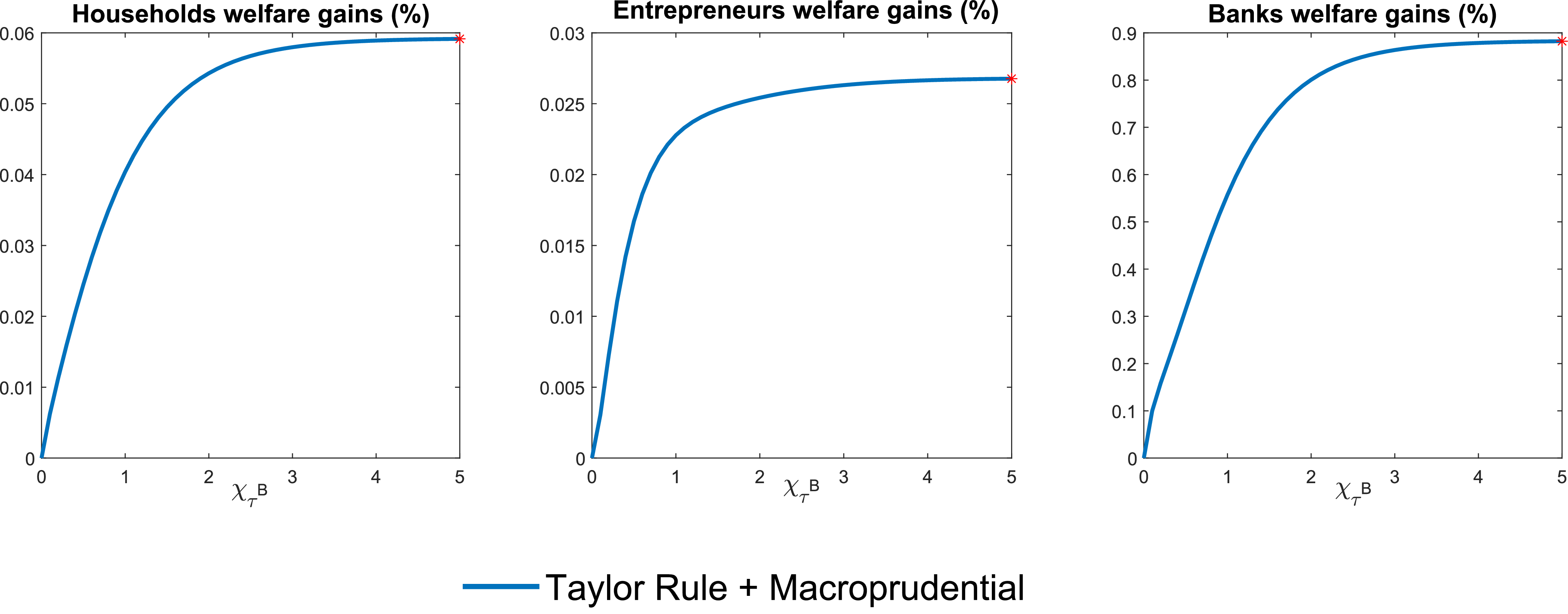
. Entrepreneurs’ welfare gains are smaller compared to those in the other shock scenarios. Figure 6 shows that entrepreneurs’ gains can be higher if the value of
 $\chi _{\tau ^B}$
is increased. The recovery of economic activity after an adverse collateral shock involves the recovery of investments made by entrepreneurs, which contributes to a faster recovery of accumulated output.
7.3 Negative financial shock
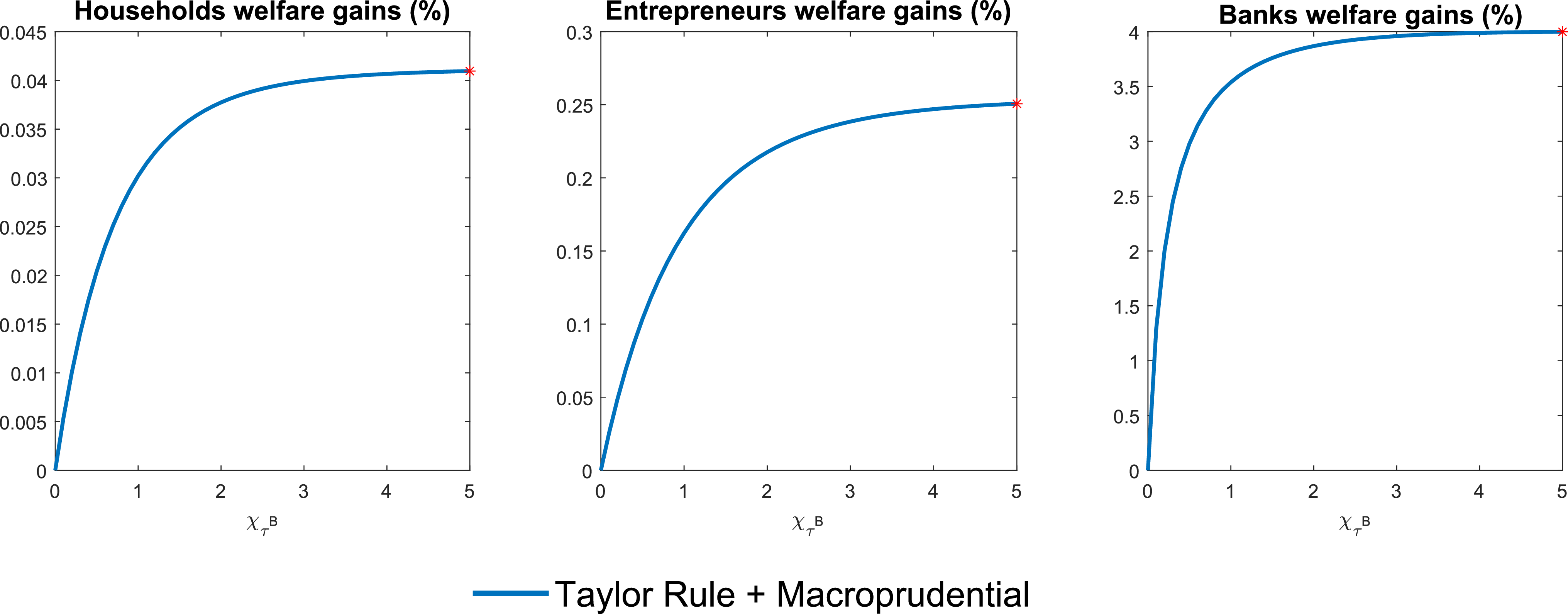
In this section, I analyze the effects of an unexpected financial shock on the welfare of the main agents of the model. Figure 7 shows that all agents benefit from the introduction of macroprudential policy, with banks benefiting particularly due to lower costs from deviating from their optimal leverage target. When a financial shock destroys the capital accumulated by banks, there is an immediate fall in the capital-to-loans ratio, which generates deviation costs (30) from the optimal target. If macroprudential policy is active, capital requirements can vary over time and reduce the difference
 $\left (\frac {k^B}{b} - \tau ^{B}_{t}\right )$
, which would otherwise increase costs following the negative financial shock.
Welfare gains with
 $\chi _{\tau ^B} \in [0,5]$
– negative financial shock.
Note: Welfare gains from introducing the macroprudential regulation, given monetary policy (different values of the loans-to-output feedback parameter in the time-varying capital requirement rule).

Welfare gains with baseline parameters – negative financial shock

 $^*$
Welfare gains compared with the baseline policy regime (only TR).
The reduction in the target allows banks to recover the capital loss more quickly and avoid charging a high loan rate. With lower credit costs, entrepreneurs can increase their investment levels, which mitigates the decline in accumulated output compared to the scenario with only monetary policy. A macroprudential policy with a strong response to deviations in the loans-to-output ratio
 $(\chi _{\tau ^B})$
leads to higher welfare gains for all agents, as shown in Figure 7.
The positive effect of macroprudential policy on banks is not observed in adverse shocks during which they accumulate additional capital, such as productivity and investment shocks. In these cases, macroprudential policy reduces the spread and the accumulation of bank capital, resulting in lower dividends
 $div^B$
and diminished welfare
 $W^B$
. By contrast, under an adverse financial shock, macroprudential policy enhances bank welfare, thereby mitigating the shock’s impact. Table 5 shows that the welfare gain with macroprudential policy is 0.29% higher than under monetary policy alone, when the economy faces an adverse financial shock of standard deviation 0.01 and macroprudential policy is calibrated at
 $\chi _{\tau ^B}=0.5$
. Households also benefit from macroprudential policy, as stabilizing output fluctuations reduces inflation and increases their real gains relative to the only monetary policy scenario.
7.4 Negative investment shock
This section analyzes the effects of an adverse shock that increases the cost of transforming old capital into new capital in the production of the wholesale good. This shock reduces the price of capital, making entrepreneurs more financially constrained and creating incentives for the Cournot banking system to raise the loan rate by reducing credit supply. As shown in Figure 4, banks are able to accumulate more capital under this shock.
Macroprudential policy plays a dual role. On the one hand, it mitigates the amplifying effect of the BS channel on the loan rate by narrowing the gap
 $\left (\frac {k^B}{b} - \tau ^{B}_{t}\right )$
in the presence of a negative investment shock, while also improving the welfare of households and entrepreneurs by reducing fluctuations in accumulated output. On the other hand, it worsens banks’ position: the spread declines, capital accumulation
 $k^B$
falls, and dividends decrease. Table 6 shows that banks experience a welfare loss of –0.40% following the introduction of macroprudential policy under a negative investment shock.
Welfare gains with baseline parameters – negative investment shock

 $^*$
Welfare gains compared with the baseline policy regime (only TR).
Welfare gains with
 $\chi _{\tau ^B} \in [0,5]$
– negative investment shock.
Note: Welfare gains from introducing the macroprudential regulation, given monetary policy (different values of the loans-to-output feedback parameter in the time-varying capital requirement rule).

Figure 8 shows that increasing the macroprudential policy feedback parameter
 $\chi _{\tau ^B}$
within the range
 $[0,5]$
further reduces the welfare gains of banks, an effect not observed for households and entrepreneurs, who benefit from the intervention of the macroprudential authority. Welfare gains can reach 0.05% for households and 0.23% for entrepreneurs if
 $\chi _{\tau ^B}$
equals the maximum value in the given range. In contrast, the increase in
 $\chi _{\tau ^B}$
implies a higher welfare loss for banks, reaching -0.48% when
 $\chi _{\tau ^B} = 5$
.
7.5 Increasing banking competition
Table 7 shows the effects of increased banking competition on agents’ welfare gains when macroprudential policy is active. Two scenarios are considered: (i) the baseline scenario with only monetary policy, and (ii) the alternative scenario with macroprudential policy active. Monetary policy feedback parameters are kept at
 $\phi _{\pi } = 1.56$
and
 $\phi _{y} = 0.33$
, while the macroprudential policy feedback parameter is set to
 $\chi _{\tau ^B} = 0.5$
. The baseline scenario also assumes the number of banks
 $N$
is five, corresponding to the five largest Brazilian banks. Tables 7 and 8 also show total welfare, an aggregate measure of the agents’ welfare in the model (households, entrepreneurs, and banks), for
 $N=15$
and
 $N=30$
. This measure is used to assess the efficiency and effectiveness of economic policies (monetary and macroprudential) and their implications for overall societal welfare.
Welfare gains with more banking competition (macroprudential policy active)
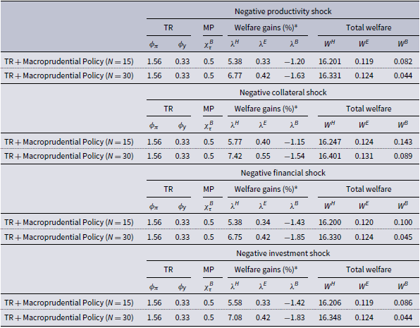
 $^{*}$
Welfare gains compared with the alternative policy regime formed by monetary and macroprudential policies with
 $N=5$
.
Welfare gains with more banking competition (only monetary policy)
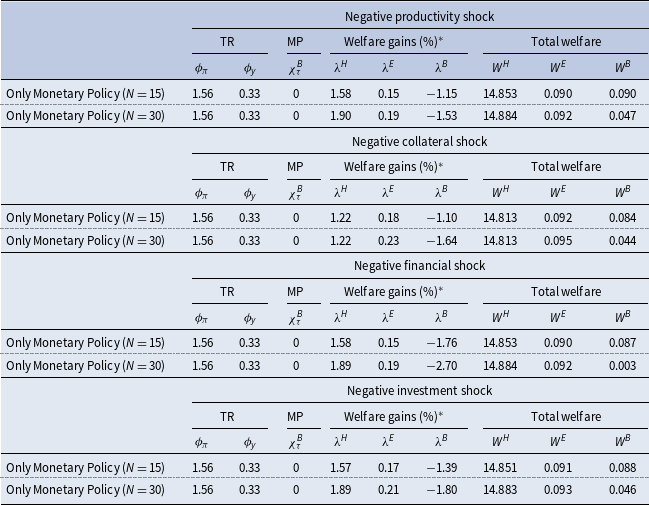
 $^{*}$
Welfare gains compared with the baseline policy regime formed by only monetary policy with
 $N=5$
.
The welfare gains for households and entrepreneurs resulting from the introduction of macroprudential policy are amplified under higher banking competition, as shown in Figure 9. If entry barriers for new banks are removed in the presence of a productivity shock, allowing competition to increase to
 $N=15$
, welfare gains are 5.38% for households and 0.33% for entrepreneurs compared to the scenario with
 $N=5$
. Further increasing banking competition to
 $N=30$
raises the welfare gains to 6.77% for households and 0.42% for entrepreneurs (Table 7).
In contrast, in the presence of a negative
 $z$
shock, banks lose welfare under increased competition when macroprudential policy is active because they accumulate less capital due to the lower spread, which in turn reduces dividends. When the loan-to-output ratio falls, the macroprudential authority can intervene by reducing capital requirements
 $\tau ^{B}$
, limiting banks’ ability to amplify the spread through the BS channel. As a result, banks’ welfare gains are lower. A similar outcome occurs for an investment shock, where banks are also unable to charge a higher spread under active macroprudential policy, leading to a welfare loss compared to the scenario with only monetary policy.
Welfare gains with
 $N \in [5,30]$
.
Note: Welfare gains from introducing the macroprudential rule, given monetary policy (different values of the number of banks).

Figure 9 shows a contrasting effect on banks’ welfare gains when banking competition increases in the presence of financial shocks. Higher competition reduces banks’ ability to adjust the loan rate by cutting loan supply when the economy is hit by shocks transmitted mainly through the IBC channel. As a result, banks accumulate less capital and pay lower dividends, thereby reducing their welfare gains. The introduction of macroprudential policy, however, helps reduce the costs that penalize banks for deviating from the optimal leverage target when an unexpected financial shock diminishes bank capital. More banking competition also implies lower profits and smaller capital buffers, which weakens banks’ capacity to absorb financial shocks. In this scenario, macroprudential policy becomes crucial for supporting banks’ financial recovery. Table 7 shows that, under macroprudential policy active, banks experience welfare losses of −1.43% when the number of banks increases to
 $N=15$
, and −1.85% when
 $N=30$
. Under the only monetary policy, welfare losses amount to −1.76% when
 $N$
rises from 5 to 15, and −2.70% when
 $N=30$
.
Macroprudential policy has a similar effect on bank welfare
 $W^B$
under an adverse collateral shock because of the associated bank capital loss. However, it is less effective in limiting the decline in bank welfare when competition increases, as shown in Figure 9. This lower effectiveness arises because the collateral shock affects the IBC channel through PED, whereas macroprudential policy acts on the BS channel. Table 7 shows that banks face a welfare loss of −1.15% when the number of banks rises to
 $N=15$
, and −1.54% when
 $N=30$
. In the only monetary policy scenario, the entry of new banks also increases households’ and entrepreneurs’ welfare gains. Equation (39) shows that more banks reduce the adverse effects of shocks transmitted through the IBC channel, thereby lowering the loan rate under imperfect competition. With cheaper credit, entrepreneurs can increase investment, raising output
 $y$
and directly improving households’ and entrepreneurs’ welfare. However, these welfare gains are smaller than under the scenario with active macroprudential policy.
In the presence of a productivity shock, increasing banking competition from
 $N=5$
to
 $N=15$
yields welfare gains of 1.58% for households and 0.15% for entrepreneurs. With further competition up to
 $N=30$
, gains increase to 1.90% for households and 0.19% for entrepreneurs (Table 8). Higher banking competition also improves
 $W^H$
and
 $W^E$
under collateral and investment shocks. However, monetary policy alone is insufficient to stabilize banks’ welfare
 $W^B$
in the face of financial shocks.
8. Banking competition and the effects of stabilization policies
This section analyzes the effects of banking competition on accumulated output and spread fluctuations. I consider three scenarios, evaluated for all adverse shocks: (i) an imperfectly competitive banking system (
 $N=5$
); (ii) reduced entry barriers (
 $N=15$
); and (iii) the scenario closest to perfect competition (
 $N=30$
). The aim is to assess how the effectiveness of monetary and macroprudential policies in mitigating business-cycle fluctuations is affected by different levels of banking competition. I consider two policy frameworks: a baseline with only monetary policy, and an alternative with macroprudential policy active. Increasing the number of banks reduces the impact on the spread for all shocks. Figure 10 shows that more banking competition further attenuates spread fluctuations when macroprudential policy is active. Fluctuations are smaller because both bank channels that amplify shocks are constrained: a larger
 $N$
limits the power of the IBC channel, while time-varying capital requirements
 $\tau ^B$
restrict the BS channel.
Impulse response to spread given different number of banks.
Note: The horizontal axis shows quarters after a negative shock at the beginning of period one. The vertical axis shows the percentage deviation from the steady state for spread. Two scenarios are considered: a baseline with only monetary policy (TR) and an alternative with macroprudential policy active (TR + MP).

Impulse response to output given different number of banks.
Note: The horizontal axis shows quarters after a negative shock at the beginning of period one. The vertical axis shows the percentage deviation from the steady state for output. Two scenarios are considered: a baseline with only monetary policy (TR) and an alternative with macroprudential policy active (TR + MP).

A negative productivity shock in the production function (9) reduces entrepreneurs’ demand for physical capital
 $k$
, and lowers the price of capital
 $q$
. The decline in
 $q$
tightens entrepreneurs’ borrowing constraint (11), making loan demand more inelastic. In the
 $N=5$
scenario this higher inelasticity amplifies the spread. Increasing banking competition to
 $N=15$
and
 $N=30$
attenuates the spread response. Figure 11 shows that the decline in output following a negative
 $z$
shock is smaller when more banks are present – because borrowing costs fall – and that active macroprudential policy further mitigates the drop in
 $y$
.
The negative collateral shock
 $m^k$
destroys the guarantees entrepreneurs provide to banks to obtain loans and makes them more financially constrained. Banks operating under imperfect competition take advantage of the more inelastic PED by reducing the supply of loans in order to raise the loan rate, thereby directly affecting the spread. The higher cost of credit used to finance entrepreneurial activity negatively impacts physical capital
 $k$
and labor hiring
 $l$
, leading to a decline in accumulated output
 $y$
. Higher banking competition reduces banks’ ability to charge higher loan rates
 $R^b$
, even when entrepreneurs are financially constrained. Thus, in the case of a collateral shock, the combination of macroprudential policy and a larger number of banks (
 $N=30$
) keeps the output deviation close to the original steady state.
Figure 11 shows that the effects of a financial shock are amplified when the banking system consists of only a few banks (
 $N=5$
) and macroprudential policy is absent. An adverse financial shock pushes the capital-to-loans ratio below the initial optimal leverage target. This movement in
 $\frac {k^B}{b}$
ratio increases the punitive costs of deviating from the optimal leverage target, and banks transfer these financial losses to entrepreneurs. The resulting increase in the loan rate raises borrowing costs, leading to a slowdown in investment and a reduction in accumulated output. When capital requirements
 $\tau ^B$
vary over time, the macroprudential authority can reduce these costs for the banking system. In this way, the influence of the BS channel on credit costs and economic activity is weakened, resulting in smaller fluctuations in both the spread and output.
Lastly, the negative investment shock affects capital producers by increasing the cost of transforming old capital into new capital used to produce wholesale goods
 $y^{w}$
, thereby causing a decline in output
 $y$
. The lower price
 $q$
makes entrepreneurs more financially constrained. Banks in imperfect competition take advantage of entrepreneurs’ financial constraints and increase the spread. An increase in the number of banks from
 $N=5$
to
 $N=30$
reduces the deviation of the spread from its initial steady state. Figure 11 shows that the introduction of macroprudential policy has little influence on reducing fluctuations in accumulated output relative to the only monetary policy scenario in the initial quarters. However, when the number of banks is high
 $(N=30)$
, accumulated output
 $y$
recovers more quickly under macroprudential policy in response to the adverse investment shock.
9. Sensitivity analysis
This section examines the robustness of the baseline results in Section 6 by varying the investment adjustment cost parameter,
 $\chi$
, and the bank capital adjustment cost parameter,
 $\kappa _{k^B}$
. The investment adjustment cost takes three values:
 $\chi _1 = 1$
,
 $\chi _2 = 5$
(the estimated value for Brazil), and
 $\chi _3 = 10$
. The bank capital adjustment cost also takes three values:
 $\kappa _{k^B,1} = 10$
,
 $\kappa _{k^B,2} = 22.19$
(the estimated value for Brazil), and
 $\kappa _{k^B,3} = 30$
. In all scenarios, macroprudential policy is active. The objective is to test different economic environments by varying these parameters within a plausible range, thereby assessing how the model responds to various economic conditions.
9.1 Investment adjustment cost
 $\chi$

Figure 12 shows that variations in the adjustment cost
 $\chi$
significantly affect the model’s main variables under negative collateral, financial, and investment shocks. In contrast, fluctuations are minimized when a negative productivity shock occurs. The adjustment cost
 $\chi$
represents the cost of transforming old capital into new capital and is the responsibility of the capital producers.
The largest divergence in the trajectories of the analyzed variables following an initial negative shock arises from an investment shock affecting capital producers. For a higher value of
 $\chi$
(
 $\chi _3 = 10$
), a negative investment shock leads to a substantial fall in the price of capital
 $q$
, constraining entrepreneurs financially since capital serves as collateral. Banks respond to this tightening of financial conditions by raising loan interest rate
 $R^b$
, which increases the spread. Under these circumstances, banks are able to accumulate more capital.
Banks can also accumulate more capital following a negative productivity shock, but increasing
 $\chi$
does not amplify fluctuations in the spread. A negative collateral shock reduces the collateral that entrepreneurs can provide to obtain loans, and higher
 $\chi$
further limits collateral availability, resulting in fewer guarantees for banks. Banks exploit this situation by charging a higher spread, pushing the economy toward a worse equilibrium with a decline in accumulated output. Finally, in the event of a financial shock affecting banks, they can charge higher interest rates if entrepreneurs are financially constrained, which occurs in scenarios with a high
 $\chi$
value.
Impulse responses to different negative shocks with variation in
 $\chi$
.
Note: The horizontal axis shows quarters after a negative shock occurring at the beginning of period one. The vertical axis shows the percentage deviation from the steady state of the analyzed variable. Macroprudential policy is active.

Impulse responses to different negative shocks with variation in
 $\kappa _{k^B}$
.
Note: The horizontal axis shows quarters after a negative shock occurring at the beginning of period one. The vertical axis shows the percentage deviation from the steady state of the analyzed variable. Macroprudential policy is active.

9.2 Bank capital adjustment cost
$\kappa _{k^B}$

Figure 13 shows the effects of different shocks that hit the economy as the bank capital adjustment cost
 $\kappa _{k^B}$
varies. The parameter
 $\kappa _{k^B}$
plays a crucial role in determining the cost
 $\Omega _B$
, as given by (30). A higher bank capital adjustment cost
 $\kappa _{k^B}$
amplifies fluctuations in the loan rate
 $R^b$
when adverse shocks are transmitted through the BS channel. These shocks directly or indirectly lead to deviations of bank capital from the optimal target set by the macroprudential authority.
An unexpected negative financial shock affects the BS channel, causing an immediate decline in the capital-to-loans ratio
 $\frac {k^B}{b}$
, which leads to an increase in the spread. When banks face higher adjustment costs (
 $\kappa _{k^B,3} = 30$
), the rise in the spread becomes more pronounced and intensifies fluctuations in real variables affected by it. As a result, a higher loan rate and reduced borrowing capacity impose financial constraints on entrepreneurs (characterized by inelastic PED), contributing to a fall in accumulated output
 $y$
as entrepreneurs slow down productive activities, hire fewer workers
 $l$
, and acquire less capital
 $k$
.
Regarding the negative investment shock, an increase in
 $\kappa _{k^B}$
also affects spread fluctuations. A higher value of
 $\kappa _{k^B}$
leads to significant fluctuations in the spread, which take more than 40 quarters to return to the initial equilibrium. In this scenario, there is a sharp decline in accumulated output, and banks accumulate more capital as the loan rate increases. Higher bank capital raises the capital-to-loans ratio
 $\frac {k^B}{b}$
during a negative investment shock. A similar pattern in the capital-to-loans ratio is observed under a negative productivity shock. In this case, banks accumulate more capital by charging higher interest rates on loans, as entrepreneurs face financial difficulties and have limited bargaining power. Accumulated output also takes approximately 40 quarters to return to its initial equilibrium after a negative productivity shock when
 $\kappa _{k^B}$
is high.
Lastly, a negative collateral shock amplifies the spread when the bank capital adjustment cost
 $\kappa _{k^B}$
is high. As entrepreneurs have less physical capital to offer as collateral, their loan demand becomes inelastic, incentivizing banks in an imperfectly competitive environment to raise the spread. However, the reduction in loan demand from entrepreneurs limits banks’ ability to expand their capital
 $k^B$
. Consequently, bank capital accumulation declines, leading to a lower capital-to-loans ratio that takes approximately 25 quarters to return to its steady state after the negative collateral shock. Moreover, the more pronounced slowdown in productive activity when
 $\kappa _{k^B}$
is high results in a sharper decline in accumulated output
 $y$
, which takes approximately 40 quarters to return to its initial equilibrium.
10. Conclusions
My paper examines the stabilization properties of macroprudential policy in an environment dominated by an oligopolistic banking system. The results show that a countercyclical macroprudential policy can stabilize business-cycle fluctuations by influencing the loan rate and, consequently, the spread. The welfare analysis indicates that macroprudential policy delivers additional welfare gains, relative to a scenario with only monetary policy, for both households and entrepreneurs when the economy is hit by different adverse shocks. Moreover, macroprudential policy mitigates the impact of the BS channel on credit costs, enabling entrepreneurs to restore productive activity, thereby stabilizing the decline in accumulated output triggered by negative shocks.
The findings show that the oligopolistic banking system recovers more quickly from unexpected capital losses in an environment with an active macroprudential policy. In the case of financial shocks that reduce banks’ capital and increase the punitive costs of deviating from the optimal leverage target, macroprudential policy mitigates these costs, enabling banks to recover financially without charging a higher spread. However, macroprudential policy generates negative welfare gains for banks under productivity and investment shocks, as it prevents them from raising spreads and accumulating additional capital. The interaction between macroprudential policy and bank dividends is complex, with effects that vary depending on the specific shocks. High inflation emerges when entrepreneurs reduce production in response to adverse macroeconomic shocks, such as productivity and investment shocks. In this context, even if banks distribute high dividends due to increased bank capital in the absence of macroprudential policy, the value of these dividends is eroded by inflation. Consequently, these dividends fail to strengthen household consumption, leading to no significant improvement in overall welfare.
The results show that if macroprudential policy is implemented in scenarios with adverse productivity and investment shocks, it improves the real side of the economy at the expense of a deterioration in the financial system. Since the primary concern of the macroprudential authority is to maintain financial stability, macroprudential policy should not be implemented for these two types of shocks under IBC. Nevertheless, macroprudential policy can strengthen the economy’s resilience to financial shocks and to shocks that reduce entrepreneurs’ collateral. The results also indicate that a higher policy response parameter to deviations in the loans-to-output ratio from its optimal target leads to lower capital requirements imposed by the macroprudential authority, and consequently, to higher welfare gains for banks when financial and collateral shocks occur. Furthermore, the results show that the effectiveness of macroprudential policy in controlling the spread is amplified in environments with higher banking competition.
This paper focuses on the Brazilian economy, given its high level of banking concentration, where a small number of banks hold a significant share of financial assets. While the model is estimated for Brazil, the underlying mechanisms – particularly the roles of IBC and BS in the transmission of shocks – are not unique to Brazil. Similar market structures can be observed in other economies, where a few banks dominate the financial system. Nevertheless, differences in financial development – such as market liquidity, regulatory frameworks, availability of financial instruments, central bank independence, and capital flow volatility – can influence the quantitative results. Therefore, the findings should be interpreted primarily as insights into economies with concentrated banking sectors that dominate a large fraction of financial assets. These characteristics are typical of many emerging markets, but also present in specific segments of advanced economies, as shown by Li (Reference Li2021). Future research could extend the framework to other financial environments to assess the robustness and external validity of the results.
The 2008 global financial crisis highlighted the need for new instruments to manage an environment in which financial shocks can amplify business-cycle fluctuations. The results of this paper indicate that macroprudential policy should not be considered a substitute for monetary policy, but rather a useful complement to address financial problems or adverse sectoral shocks and to improve welfare. Macroprudential policy is a more effective tool for financial stabilization than monetary policy, as it operates directly on the supply of credit, an important driver of macroeconomic dynamics.
Acknowledgements
The author would like to thank the editor, Professor William A. Barnett, and two anonymous referees for their valuable comments and helpful editorial suggestions. The author also thanks Pierluca Pannella, Soraya Roman, and José Angelo Divino for insightful comments and suggestions that significantly improved the content and presentation of the paper.
Competing interests
The author declares no competing interests.
Appendices
A. Entrepreneurs’ optimization problem
The entrepreneur’s objective is to maximize the expected lifetime utility:
 \begin{align} \mathbb{E}_t \sum _{s=0}^{\infty } (\beta ^E)^{s} \ln \big(c^{E}_{t+s}\big) \end{align}
subject to the budget constraint:
 \begin{align} c_{t}^{E} + q_t k_{t} + w_t l_t + \dfrac {R^{b}_{t-1} b_{t-1}}{\pi _t}= \dfrac {y^{w}_{t}}{x_t} +(1-\delta ) q_t k_{t-1} + b_t \end{align}
and subject to the borrowing constraint:
 \begin{align} b_t \leq m^{k}_{t} \mathbb{E}_t \left [\dfrac { q_{t+1} (1-\delta ) k_{t}\pi _{t+1}}{R^{b}_{t}} \right ] \end{align}
which
 $m^{k}_{t} \in (0, 1)$
denotes the fraction of physical capital collateral that can be confiscated by banks when the entrepreneurs fail to repay their debt. The Lagrangian can be written as:
 \begin{align} \mathcal{L} &= \mathbb{E}_t \sum _{s=0}^{\infty } (\beta ^{E})^{s} \ln \big(c_{t+s}^{E}\big) - \lambda _{1,t}^{E}\!\left \{c_t^{E} + q_t k_t + w_t l_t + \frac {R^{b}_{t-1} b_{t-1}}{\pi _t} - \frac {y_t^{w}}{x_t} - (1-\delta ) q_t k_{t-1} - b_t\right \} \notag \\ &\quad - \lambda _{2,t}^{E}\!\left \{b_t - m_t^{k}\mathbb{E}_t\!\left [\frac {q_{t+1} k_t (1-\delta )\pi _{t+1}}{R_t^{b}}\right ]\right \} \end{align}
The first-order conditions are:
 \begin{align} \big(c_t^{E}\big)\, :\quad \frac {1}{c_t^{E}} - \lambda _{1,t}^{E} &= 0 \notag \\ \lambda _{1,t}^{E} &= \frac {1}{c_t^{E}} \end{align}
 \begin{align} (b_t)\, :\quad \lambda _{1,t}^{E}- \beta ^E \mathbb{E}_t\!\left [ \lambda _{1,t+1}^{E} \frac {R_t^{b}}{\pi _{t+1}}\right ]- \lambda _{2,t}^{E} &= 0 \notag \\ \lambda _{2,t}^{E} &=\lambda _{1,t}^{E}- \beta ^E \mathbb{E}_t\!\left [\lambda _{1,t+1}^{E} \frac {R_t^{b}}{\pi _{t+1}}\right ] \end{align}
 \begin{align} (l_t):\quad - \lambda _{1,t}^{E} w_t+ \lambda _{1,t}^{E} (1-\alpha )\frac {z_t (k_{t-1})^\alpha l_t^{-\alpha }}{x_t}\dfrac {l_{t}}{l_{t}}&= 0 \notag \\ w_t &= (1-\alpha )\frac {y_t^{w}}{x_t l_t} \end{align}
 \begin{eqnarray} (k_{t}): -\lambda _{1,t}^{E} q_{t} + \beta ^E \mathbb{E}_t \left [ \lambda _{1,t+1}^{E} \frac { \alpha z_{t+1} (k_{t})^{\alpha -1} (l_{t+1})^{1-\alpha }}{x_{t+1}} \dfrac {k_{t}}{k_{t}}\right ]+ \beta ^E \mathbb{E}_t \big[ \lambda _{1,t+1}^{E}(1-\delta ) q_{t+1}\big] \nonumber \\ + \lambda _{2,t}^{E} m^{k}_{t} \mathbb{E}_t \left [\frac {(1-\delta )q_{t+1} \pi _{t+1}} {R^{b}_{t}} \right ] = 0 \nonumber \\ \lambda _{1,t}^{E} q_{t} = \beta ^E \mathbb{E}_t \left [\lambda _{1,t+1}^{E} \left (\alpha \frac {y^{w}_{t+1}}{x_{t+1} k_{t}} + (1-\delta ) q_{t+1} \right )\right ] + \lambda _{2,t}^{E} m^{k}_{t} \mathbb{E}_t \left [ \frac {(1-\delta )q_{t+1} \pi _{t+1}}{R^{b}_{t}} \right ] \end{eqnarray}
It is possible to find an expression for
 $(k_{t}$
) replacing (55) and (56) in (58):
 \begin{align} \frac {q_t}{c_t^{E}} &=\beta ^E \mathbb{E}_t\!\left [\frac {1}{c_{t+1}^{E}} \left (\alpha \frac {y_{t+1}^{w}}{x_{t+1} k_t} + (1-\delta ) q_{t+1}\right )\right ] \notag \\ &\quad + \left (\frac {1}{c_t^{E}} - \beta ^E \mathbb{E}_t\!\left [\frac {R_t^{b}}{c_{t+1}^{E} \pi _{t+1}}\right ]\right ) m_t^{k}\mathbb{E}_t\!\left [\frac {(1-\delta ) q_{t+1} \pi _{t+1}}{R_t^{b}}\right ] \end{align}
B. Banks’ optimization problem
Banks maximize the dividends paid to shareholders (households). The optimization problem of bank
 $j$
is:
 \begin{align} \begin{aligned} \max _{\{b_t(j), k^{B}_{t}(j), div_{t}^{B}(j)\}} \quad & \mathbb{E}_t \sum _{s=0}^{\infty } \Lambda _{t,t+s} \big[\ln (div_{t+s}^{B} (j))\big]\\[5pt] \textrm {s.t.} \quad &k_{t}^{B} (j) = (1-\delta ^B) k_{t-1}^{B}(j) + \Gamma _{t}^{B} (j) - div_{t}^{B}(j) \\[5pt] & div_{t}^{B} (j) \geq 0 \\[5pt] &k_{t}^{B}(j) \geq 0 \\[5pt] & b_t(j) \geq 0 \end{aligned} \end{align}
The Lagrangian is:
 \begin{align} \mathcal{L} = \sum _{s=0}^{\infty } \Lambda _{t,t+1} \mathbb{E}_t\!\left \{\ln \big (div_t^{B}(j)\big ) + \lambda _t^{B}(j)\!\left [k_t^{B}(j) + div_t^{B}(j) - (1-\delta ^{B}) k_{t-1}^{B}(j) - \Gamma _t^{B}(j) \right ]\right \} \end{align}
The first-order conditions are as follows:
 \begin{align} (div_t^{B}(j)) \, :\quad \frac {1}{div_t^{B}(j)} + \lambda _t^{B}(j) &= 0 \notag \\ \lambda _t^{B}(j) &= - \frac {1}{div_t^{B}(j)} \end{align}
 \begin{align} (b_t(j)) \, :\quad \mathbb{E}_t \Lambda _{t,t+1} \left \{\dfrac {\lambda _{t+1}^{B}(j)}{\pi _{t+1}} \left [\dfrac {\partial \Omega _{t}^{B}(j)}{\partial b_t(j)} - \left ( \dfrac {\partial R_{t}^{b}}{\partial b_t(j)} b_t(j) + R_{t}^{b} - R_{t}^{d}\right )\right ] \right \}&= 0 \end{align}
 \begin{align} \big(k_t^{B}(j)\big)\,:\quad \lambda _t^{B}(j) + \mathbb{E}_t \Lambda _{t,t+1} \lambda _{t+1}^{B}(j) \left \{\frac {1}{\pi _{t+1}}\left [\frac {\partial \Omega _t^{B}(j)}{\partial k_t^{B}(j)} - R_t^{d}\right ] - (1-\delta ^{B}) \right \} &= 0 \end{align}
Using
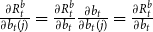 $\frac {\partial R_{t}^{b}}{\partial b_t(j)} = \frac {\partial R_{t}^{b}}{\partial b_t } \frac {\partial b_t}{\partial b_t(j)} = \frac {\partial R_{t}^{b}}{\partial b_t }$
in (63), we obtain the following expression:
 \begin{align} \frac {\partial \Omega _t^{B}(j)}{\partial b_t(j)} - \left (\frac {\partial R_t^{b}}{\partial b_t(j)} b_t(j) + R_t^{b} - R_t^{d}\right ) &= 0 \notag \\[4pt] \frac {\partial \Omega _t^{B}(j)}{\partial b_t(j)}- \left (\frac {\partial R_t^{b}}{\partial b_t} \frac {b_t}{N}+ R_t^{b} - R_t^{d}\right ) &= 0 \notag \\[4pt] \frac {\partial \Omega _t^{B}(j)}{\partial b_t(j)} - \left (\frac {\partial R_t^{b}}{\partial b_t} \frac {b_t}{R_t^{b}} \frac {1}{N} + 1\right ) R_t^{b} + R_t^{d} &= 0 \notag \\[4pt] \frac {\partial \Omega _t^{B}(j)}{\partial b_t(j)} - \left (1 - PED_t^{-1} \frac {1}{N}\right ) R_t^{b}+ R_t^{d} &= 0 \end{align}
By isolating
 $R_{t}^{b}$
and using
 $b_t = b_t(j) N$
and
 $k_{t}^{B} = k_{t}^{B}(j) N$
, the loan interest rate
 $R_{t}^{b}$
can be expressed as:
 \begin{align} R_t^{b} &=\frac {R_t^{d} + \dfrac {\partial \Omega _t^{B}(j)}{\partial b_t(j)}} {\left (1 - PED_t^{-1}\dfrac {1}{N}\right )} \notag \\ R_t^{b} &=\frac {R_t^{d} - \kappa _{k^B}\!\left (\dfrac {k_t^{B}(j)}{b_t(j)} - \tau _t^{B}\right )\left (\dfrac {k_t^{B}(j)}{b_t(j)}\right )^2}{\left (1 - PED_t^{-1}\dfrac {1}{N}\right )} \notag \\ R_t^{b} &=\frac {R_t^{d} - \kappa _{k^B}\!\left (\dfrac {k_t^{B}}{b_t} - \tau _t^{B}\right ) \left (\dfrac {k_t^{B}}{b_t}\right )^2}{\left (1 - PED_t^{-1}\dfrac {1}{N}\right )} \end{align}
C. Calculating the elasticity of loan demand to the loan rate (PED)
The PED can be calculated from (59). Rearranging the terms in (59):
 \begin{align} \frac {q_t}{c_t^{E}} &=\beta ^E \mathbb{E}_t\!\left [\frac {1}{c_{t+1}^{E}}\left (\alpha \frac {y_{t+1}^{w}}{x_{t+1} k_t} + (1-\delta ) q_{t+1}\right )\right ] + \frac {1}{c_t^{E}} m_t^{k}\mathbb{E}_t\!\left [\frac {q_{t+1}(1-\delta )\pi _{t+1}}{R_t^{b}}\right ] \notag \\[5pt] &\quad - \beta ^E \mathbb{E}_t\!\left [\frac {1}{c_{t+1}^{E}} \frac {R_t^{b}}{\pi _{t+1}}\right ] m_t^{k}\mathbb{E}_t\!\left [\frac {q_{t+1}(1-\delta )\pi _{t+1}}{R_t^{b}}\right ] \end{align}
Since
 $ R^{b}_{t}$
is known at time
 $ t$
, we can treat it as a constant inside the conditional expectation. Hence, (67) can be rewritten as:
 \begin{align} \frac {q_t}{c_t^{E}} &=\beta ^E \mathbb{E}_t\!\left [\frac {1}{c_{t+1}^{E}} \left (\alpha \frac {y_{t+1}^{w}}{x_{t+1} k_t} + (1-\delta ) q_{t+1}\right )\right ] + \frac {1}{c_t^{E}} m_t^{k}\mathbb{E}_t\!\left [\frac {q_{t+1}(1-\delta )\pi _{t+1}}{R_t^{b}}\right ] \notag \\ &\quad - \beta ^E \mathbb{E}_t\!\left [\frac {1}{c_{t+1}^{E}\pi _{t+1}}\right ]m_t^{k} \mathbb{E}_t\!\left [q_{t+1}(1-\delta )\pi _{t+1}\right ] \end{align}
Equation (68) can be rearranged as follows:
 \begin{align} \frac {1}{c_t^{E}}\left (q_t - m_t^{k}\mathbb{E}_t\!\left [\frac {q_{t+1}(1-\delta )\pi _{t+1}}{R_t^{b}}\right ]\right ) &=\beta ^E \mathbb{E}_t\!\left [\frac {1}{c_{t+1}^{E}}\left (\alpha \frac {y_{t+1}^{w}}{x_{t+1} k_t} + (1-\delta ) q_{t+1}\right )\right ] \notag \\ &\quad - \beta ^E \mathbb{E}_t\!\left [\frac {1}{c_{t+1}^{E}\pi _{t+1}}\right ]m_t^{k} \mathbb{E}_t\!\left [q_{t+1}(1-\delta )\pi _{t+1}\right ] \end{align}
 \begin{align} q_t - m_t^{k} \mathbb{E}_t\!\left [\frac {q_{t+1}(1-\delta )\pi _{t+1}}{R_t^{b}}\right ] &= \beta ^E \mathbb{E}_t\!\left [\frac {c_t^{E}}{c_{t+1}^{E}}\frac {\alpha z_{t+1} (l_{t+1})^{1-\alpha }}{x_{t+1}}\right ] (k_t)^{\alpha -1} \notag \\ &\quad + \beta ^E \mathbb{E}_t\!\left [\frac {c_t^{E}}{c_{t+1}^{E}} (1-\delta ) q_{t+1} \right ] \notag \\ &\quad - \beta ^E \mathbb{E}_t\!\left [\frac {c_t^{E}}{c_{t+1}^{E}\pi _{t+1}}\right ] m_t^{k}\mathbb{E}_t\!\left [q_{t+1}(1-\delta )\pi _{t+1}\right ] \end{align}
Define now:
 \begin{align} A_{k,t} &\equiv q_t - m_t^{k}\mathbb{E}_t\!\left [\frac {q_{t+1}(1-\delta )\pi _{t+1}}{R_t^{b}}\right ] \end{align}
 \begin{align} B_{k,t} &\equiv \beta ^E \mathbb{E}_t\!\left [\frac {c_t^{E}}{c_{t+1}^{E}}\frac {\alpha z_{t+1} (l_{t+1})^{1-\alpha }}{x_{t+1}}\right ] \gt 0 \end{align}
 \begin{align} C_{k,t} &\equiv \beta ^E \mathbb{E}_t\!\left [\frac {c_t^{E}}{c_{t+1}^{E}} (1-\delta ) q_{t+1} \right ] - \beta ^E \mathbb{E}_t\!\left [\frac {c_t^{E}}{c_{t+1}^{E}\pi _{t+1}}\right ] m_t^{k}\mathbb{E}_t\!\left [q_{t+1}(1-\delta )\pi _{t+1}\right ] \end{align}
Note that
 $B_{k,t} \gt 0$
is guaranteed by the properties of the model:
 $\alpha \gt 0$
,
 $c_t^E \gt 0$
,
 $l_{t+1} \gt 0$
,
 $x_{t+1} \gt 0$
, and the productivity
 $z_{t+1} \gt 0$
as implied by the production function (9) and the AR(1) process governing
 $z_t$
. Then, we can write (70) as:
 \begin{align} A_{k,t} = B_{k,t} (k_{t})^{\alpha -1} + C_{k,t} \end{align}
Rewriting (74) to express capital
 $k_t$
explicitly:
 \begin{align} \frac {A_{k,t} - C_{k,t}}{B_{k,t}} &= (k_t)^{\alpha -1} \notag \\ \left (\frac {A_{k,t} - C_{k,t}}{B_{k,t}}\right )^{\frac {1}{\alpha -1}} &= k_t \end{align}
Since
 $R_{t}^{b}$
appears in
 $A_{k,t}$
, we differentiate (75) with respect to
 $R_{t}^{b}$
:
 \begin{align} \dfrac {\partial k_{t} }{\partial R_{t}^{b}} = \dfrac {1}{\alpha -1} \left ( \dfrac {A_{k,t} - C_{k,t}}{B_{k,t}} \right )^{\frac {1}{\alpha -1}-1} \left ( \dfrac {\partial A_{t,k}}{\partial R_{t}^{b}} \dfrac {1}{B_{k,t}} \right ) \end{align}
The derivative of
 $A_{k,t}$
with respect to
 $R_{t}^{b}$
is given by:
 \begin{align} \dfrac {\partial A_{t,k} }{\partial R_{t}^{b}} = m^{k}_{t}\mathbb{E}_t \left [ \frac {q_{t+1}(1-\delta )\pi _{t+1}}{\big(R^{b}_{t}\big)^2} \right ] \equiv D_{k,t} \gt 0 \end{align}
Note that
 $D_{k,t} \gt 0$
follows directly from the properties of the model:
 $m^k_t \gt 0$
,
 $q_{t+1} \gt 0$
,
 $(1-\delta ) \gt 0$
,
 $\pi _{t+1} \gt 0$
, and the squared loan rate
 $(R^b_t)^2 \gt 0$
. Since the conditional expectation preserves positivity,
 $D_{k,t}$
must be strictly positive. Hence, substituting
 $u_1 = \tfrac {1}{\alpha -1} \lt 0$
for
 $0\lt \alpha \lt 1$
into (76), we obtain:
 \begin{align} \frac {\partial k_t}{\partial R_t^{b}} &=u_1 \left (\frac {A_{k,t} - C_{k,t}}{B_{k,t}}\right )^{u_1-1}\left (\frac {D_{k,t}}{B_{k,t}}\right ) \notag \\ &=u_1 \left (\frac {A_{k,t} - C_{k,t}}{B_{k,t}}\right )^{u_1}\left (\frac {A_{k,t} - C_{k,t}}{B_{k,t}}\right )^{-1}\left (\frac {D_{k,t}}{B_{k,t}}\right ) \notag \\ &=u_1 \left (\frac {A_{k,t} - C_{k,t}}{B_{k,t}}\right )^{u_1}\left (\frac {D_{k,t}}{A_{k,t} - C_{k,t}}\right ) \notag \\ &=u_1 \left (\frac {D_{k,t}}{A_{k,t} - C_{k,t}}\right ) k_t \lt 0 \end{align}
where
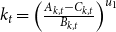 $k_t = \left ( \frac {A_{k,t} - C_{k,t}}{B_{k,t}} \right )^{u_1}$
. The derivative is negative since
 $u_1 \lt 0$
,
 $D_{k,t} \gt 0$
(as established in (77)), and
 $A_{k,t} - C_{k,t} \gt 0$
. The latter condition is guaranteed by (74), which yields:
 \begin{align} A_{k,t} - C_{k,t} = B_{k,t} \,(k_{t})^{\alpha -1} \gt 0, \end{align}
where
 $B_{k,t} \gt 0$
(as shown in (72)) and
 $k_t \gt 0$
.
Finally, the loan demand
 $b_t$
is downward-sloping with respect to the loan rate
 $R_{t}^{b}$
. To demonstrate this and to derive the price elasticity of loan demand,
 $PED_t$
, we define:
 \begin{align} PED_t \equiv -\dfrac {\partial b_t}{\partial R_{t}^{b}} \cdot \dfrac {R_{t}^{b}}{b_t} \end{align}
We begin by considering the binding borrowing constraint faced by entrepreneurs, which is defined as:
 \begin{align} b_t = m^{k}_{t} \mathbb{E}_t \left [\dfrac { q_{t+1} (1-\delta ) k_{t} \pi _{t+1} }{R^{b}_{t}} \right ] = \left (\dfrac {1}{R^{b}_{t}} \right ) m^{k}_{t} \mathbb{E}_t [q_{t+1} (1-\delta ) k_{t} \pi _{t+1}] \end{align}
Taking the derivative of
 $b_t$
with respect to
 $R_{t}^{b}$
in (81), we obtain:
 \begin{align} \frac {\partial b_t}{\partial R_t^{b}} &= - \left (\frac {1}{(R_t^{b})^2}\right ) m_t^{k} \mathbb{E}_t\!\left [q_{t+1}(1-\delta ) k_t \pi _{t+1}\right ] + \left (\frac {1}{R_t^{b}}\right ) m_t^{k} \mathbb{E}_t\!\left [q_{t+1}(1-\delta )\pi _{t+1}\right ] \left (\frac {\partial k_t}{\partial R_t^{b}}\right ) \notag \\ &= - \left (\frac {1}{R_t^{b}}\right ) m_t^{k}\mathbb{E}_t\!\left [ \frac {q_{t+1}(1-\delta ) k_t \pi _{t+1}}{R_t^{b}}\right ] + m_t^{k} \mathbb{E}_t\!\left [\frac {q_{t+1}(1-\delta )\pi _{t+1}}{R_t^{b}}\right ] \left (\frac {\partial k_t}{\partial R_t^{b}}\right ) \notag \\ &= - \frac {b_t}{R_t^{b}}+ m_t^{k} \mathbb{E}_t\!\left [\frac {q_{t+1}(1-\delta )\pi _{t+1}}{R_t^{b}}\right ]\left (\frac {\partial k_t}{\partial R_t^{b}}\right ) \end{align}
Since, as shown in (78), we have
 $\frac {\partial k_{t}}{\partial R_{t}^{b}} \lt 0$
, it follows that:
 \begin{align} \dfrac {\partial b_t}{\partial R_{t}^{b}} = -\dfrac {b_t}{R^{b}_{t}} + m^{k}_{t} \mathbb{E}_t \left [\dfrac { q_{t+1} (1-\delta ) \pi _{t+1}}{R^{b}_{t}} \right ] \dfrac { \partial k_{t}}{\partial R_{t}^{b}} \lt 0 \end{align}
 \begin{align} PED_t &= - \frac {R_t^{b}}{b_t}\left [- \frac {b_t}{R_t^{b}}+ m_t^{k} \mathbb{E}_t\!\left [ \frac {q_{t+1}(1-\delta )\pi _{t+1}}{R_t^{b}}\right ]\left (\frac {\partial k_t}{\partial R_t^{b}}\right )\right ] \notag \\ &=1 - \frac {R_t^{b}}{b_t}\left [m_t^{k} \mathbb{E}_t\!\left [\frac {q_{t+1}(1-\delta )\pi _{t+1}}{R_t^{b}}\right ]\left (\frac {\partial k_t}{\partial R_t^{b}}\right ) \right ] \notag \\ &=1 - \frac {R_t^{b}}{b_t}\left [m_t^{k} \mathbb{E}_t\!\left [\frac {q_{t+1}(1-\delta )\pi _{t+1}}{R_t^{b}}\right ]\frac {k_t}{k_t}\left (\frac {\partial k_t}{\partial R_t^{b}}\right )\right ] \notag \\ &=1 - \frac {R_t^{b}}{b_t} \frac {b_t}{k_t}\left (\frac {\partial k_t}{\partial R_t^{b}}\right ) \notag \\ &=1 + PEK_t \gt 0 \end{align}
where
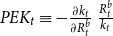 $PEK_t \equiv - \frac {\partial k_{t}}{ \partial R^{b}_{t}} \ \frac {R^{b}_{t}}{k_{t}}$
denote the elasticity of entrepreneurs’ capital demand to the loan rate. The
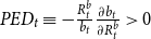 $PED_t \equiv - \frac {R_{t}^{b}}{b_t} \frac {\partial b_t}{\partial R_{t}^{b}} \gt 0$
because
 $\frac {\partial b_t}{\partial R_{t}^{b}}\lt 0$
and the entrepreneurs’ demand for capital decreases as the loan rate increases,
 $\frac { \partial k_{t}}{\partial R_{t}^{b}} \lt 0$
. Alternatively, the loan demand elasticity (
 $PED_t$
) can be expressed as a function of the marginal product of capital (
 $MPK_t$
). To do so, we first define the marginal product of capital:
 \begin{align} MPK_t \equiv \dfrac {\alpha z_t (k_{t-1})^{\alpha -1} (l_t)^{1-\alpha }}{x_t} \end{align}
and the stochastic discount factor for entrepreneurs:
 \begin{align} \Lambda _{t,t+1}^{E} \equiv \beta ^E \dfrac {u' \big(c_{t+1}^{E}\big)}{u' \big(c_{t}^{E}\big)} = \beta ^E \dfrac {c_{t}^{E}}{c_{t+1}^{E}} \end{align}
Thus, the elasticity of entrepreneurs’ capital demand with respect to the loan rate can be written as:
 \begin{align} PEK_t \equiv -\dfrac {\partial k_{t} }{\partial R_{t}^{b}} \dfrac { R_{t}^{b}}{k_{t}}= - u_1 \left ( \dfrac { D_{k,t}}{A_{k,t} - C_{k,t}} \right ) k_{t} \dfrac { R_{t}^{b}}{k_{t}} = - u_1 \left ( \dfrac { D_{k,t}}{A_{k,t} - C_{k,t}} \right ) R_{t}^{b} \end{align}
where
 $u_1 = \frac {1}{\alpha -1}\lt 0$
. Substituting
 $A_{k,t}-C_{k,t} = B_{k,t} (k_t)^{\alpha -1}$
in (87), we can equivalently write:
 \begin{align} PEK_t &= - u_1 \left ( \frac {D_{k,t}}{B_{k,t} (k_t)^{\alpha -1}} \right ) R_t^{b} \notag \\ &= - u_1 \left (\frac { m_t^{k}\mathbb{E}_t \!\left [ \frac {q_{t+1}(1-\delta )\pi _{t+1}}{(R_t^{b})^2} \right ] }{ \beta ^E \mathbb{E}_t \!\left [ \frac {c_t^{E}}{c_{t+1}^{E}} \frac {\alpha z_{t+1} (l_{t+1})^{1-\alpha }}{x_{t+1}} \right ] (k_t)^{\alpha -1} } \right ) R_t^{b} \end{align}
Using
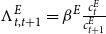 $\Lambda _{t,t+1}^{E} = \beta ^E \frac {c_{t}^{E}}{c_{t+1}^{E}}$
and
 $MPK_{t+1} = \frac {\alpha z_{t+1} (k_{t})^{\alpha -1} (l_{t+1})^{1-\alpha } }{x_{t+1}}$
in (88), we get:
 \begin{align} PEK &=- u_1 \left (\frac { m_t^{k}\mathbb{E}_t \!\left [ \frac {q_{t+1}(1-\delta )\pi _{t+1}}{(R_t^{b})^2} \right ] }{ \mathbb{E}_t \!\left [ \Lambda _{t,t+1}^{E} MPK_{t+1} \right ] } \right ) R_t^{b} \notag \\ &=- u_1 \left (\frac { m_t^{k}\mathbb{E}_t \!\left [ \frac {q_{t+1}(1-\delta )\pi _{t+1}}{R_t^{b}} \right ] }{ \mathbb{E}_t \!\left [ \Lambda _{t,t+1}^{E} MPK_{t+1} \right ] } \right ) \end{align}
Substituting
 $ u_1 = \frac {1}{\alpha -1}$
into the (89), we obtain:
 \begin{align} PEK = \dfrac {1}{1-\alpha } \left ( \dfrac { m^{k}_{t}\mathbb{E}_t \left [ \dfrac {q_{t+1}(1-\delta )\pi _{t+1}}{R^{b}_{t}} \right ] }{ \mathbb{E}_t \left [\Lambda _{t,t+1}^{E} MPK_{t+1} \right ]} \right ) \gt 0 \end{align}
It can be seen that
 $PEK_t$
depends positively on
 $m^{k}_{t}$
and on the expected discounted value of future capital prices,
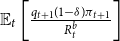 $\mathbb{E}_t \left [ \frac {q_{t+1}(1-\delta ) \pi _{t+1}}{R^{b}_{t}} \right ]$
. Furthermore,
 $PEK_t$
depends negatively on the expected discounted value of the marginal product of capital,
 $\mathbb{E}_t \left [\Lambda _{t,t+1}^{E} MPK_{t+1} \right ]$
. Replacing (90) into (84), we obtain:
 \begin{align} PED_t = 1 + \dfrac {1}{1-\alpha } \left ( \dfrac { m^{k}_{t}\mathbb{E}_t \left [ \dfrac {q_{t+1}(1-\delta )\pi _{t+1}}{R^{b}_{t}} \right ] }{ \mathbb{E}_t \left [\Lambda _{t,t+1}^{E} MPK_{t+1} \right ]} \right )\gt 0 \end{align}
It follows that the loan demand elasticity
 $PED_t$
decreases when the expected discounted marginal product of capital,
 $\mathbb{E}_t \left [\Lambda _{t,t+1}^{E} MPK_{t+1}\right ]$
, is higher or when the expected discounted value of future capital prices,
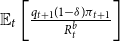 $\mathbb{E}_t \left [\frac {q_{t+1}(1-\delta )\pi _{t+1}}{R^{b}_{t}}\right ]$
, is lower. Moreover, a reduction in
 $m^k_t$
(e.g., following a negative collateral shock) lowers
 $PED_t$
both directly and indirectly: with smaller loan limits, entrepreneurs invest less, which reduces capital accumulation and raises
 $MPK_{t+1}$
, further diminishing the
 $PED_t$
.
D. Welfare gains
The unconditional welfare measure
 $W_0$
is defined as follows:
 \begin{align} W_0 = \mathbb{E} \sum _{t=0}^{\infty } \beta ^t [ U(c_t, l_t)] \end{align}
where
 $U(c_{t},l_{t})$
is the utility function, which depends on consumption
 $c_t$
and labor hours
 $l_t$
. According to Schmitt-Grohé and Uribe (Reference Schmitt-Grohé and Uribe2007) and Benigno and Woodford (Reference Benigno and Woodford2012), different policies are associated with different stochastic steady states. Therefore, I neglect the transitional dynamics leading to the stochastic steady state when using the unconditional welfare measure. It is also useful to quantify the welfare differences between macroprudential policy and the baseline policy rule (monetary policy only). As a welfare measure, the unconditional expected utilities of households, entrepreneurs, and banks in period zero are calculated:
 \begin{align} \mathbb{E}_0 W^{H} &=\mathbb{E}_0 \sum _{s=0}^{\infty } \beta \left [ \ln (c_{t+s}) + \phi _l \ln (1-l_{t+s}) \right ] \end{align}
 \begin{align} \mathbb{E}_0 W^{E} &=\mathbb{E}_0 \sum _{s=0}^{\infty } \beta ^{E}\left [ \ln (c_{t+s}^{E}) \right ] \end{align}
 \begin{align} \mathbb{E}_0 W^{B} &=\mathbb{E}_0 \sum _{s=0}^{\infty } \beta \left [ \ln (div^{B}_{t+s}) \right ] \end{align}
The desirability of a policy regime is typically evaluated by computing the compensating fraction of steady-state consumption,
 $\lambda$
, required to equate welfare in the baseline scenario (TR) with welfare under the alternative regime (MP). Accordingly,
 $\lambda$
satisfies the following equation:
 \begin{align} \mathbb{E}_t \sum _{s=0}^{\infty } \beta ^s U \left ( (1+\lambda ) c^{TR}_{t+s}, l^{TR}_{t+s} \right ) = W^{MP}_{t} \end{align}
where
 $\{c^{TR}_{t}, l^{TR}_{t}\}_{t=0}^{\infty }$
denote consumption and labor in the baseline scenario, and
 $W^{MP}_{t}$
is the welfare under the macroprudential rule. It follows that:
 \begin{align} \mathbb{E}_t \left \{ \sum _{s=0}^{\infty } \beta ^s \left [U\left ((1 +\lambda ) c^{TR}_{t+s}, l^{TR}_{t+s}\right ) - U \left ( c^{TR}_{t+s}, l^{TR}_{t+s}\right ) \right ] \right \} = W^{MP}_{t} - W^{TR}_{t} \end{align}
where
 $W^{TR}_{t}$
denotes welfare in the baseline scenario, and rewriting the terms using the paper’s log-utility function for households, we have:
 \begin{align} \mathbb{E}_t \Bigg \{\sum _{s=0}^{\infty } \beta ^s \Big [&\ln \big ((1+\lambda )c_{t+s}\big ) + \phi _l \ln (1-l_{t+s}) \notag \\ &- \ln (c_{t+s})- \phi _l \ln (1-l_{t+s})\Big ] \Bigg \}= W^{MP,H}_{t} - W^{TR,H}_{t} \notag \\[0.3cm] \mathbb{E}_t \Bigg \{ \sum _{s=0}^{\infty } \beta ^s \Big [&\ln \!\big ((1+\lambda )c_{t+s}\big ) - \ln (c_{t+s})\Big ] \Bigg \}= W^{MP,H}_{t} - W^{TR,H}_{t} \nonumber \\[0.3cm] \frac {1}{1-\beta }\Big \{&\ln (1+\lambda ) + \ln (c_{t+s}) - \ln (c_{t+s})\Big \} = W^{MP,H}_{t} - W^{TR,H}_{t}. \end{align}
It follows that:
 \begin{align} \ln (1+\lambda ) &= (1-\beta )\left (W_t^{MP,H} - W_t^{TR,H}\right ) \notag \\ 1+\lambda &= \exp \!\left [(1-\beta )\left (W_t^{MP,H} - W_t^{TR,H}\right )\right ] \notag \\ \lambda &= \exp \!\left [(1-\beta )\left (W_t^{MP,H} - W_t^{TR,H}\right )\right ] - 1 \end{align}
The same reasoning applies to entrepreneurs:
 \begin{align} \mathbb{E}_t \left \{\sum _{s=0}^{\infty } (\beta ^{E})^s \left [\ln \big ((1+\lambda )c_{t+s}^{E}\big ) - \ln \big(c_{t+s}^{E}\big) \right ]\right \}&= W_t^{MP,E} - W_t^{TR,E} \notag \\ \frac {1}{1-\beta ^{E}}\left \{\ln (1+\lambda ) + \ln \big(c_{t+s}^{E}\big) - \ln \big(c_{t+s}^{E}\big) \right \}&= W_t^{MP,E} - W_t^{TR,E} \notag \\ \ln (1+\lambda )&= (1-\beta ^{E})\left (W_t^{MP,E} - W_t^{TR,E}\right ) \notag \\ 1+\lambda &= \exp \!\left [(1-\beta ^{E})\left (W_t^{MP,E} - W_t^{TR,E}\right )\right ] \notag \\ \lambda &= \exp \!\left [(1-\beta ^{E})\left (W_t^{MP,E} - W_t^{TR,E}\right )\right ] - 1 \end{align}
Lastly, welfare gains for banks can be written as:
 \begin{align} \mathbb{E}_t \left \{\sum _{s=0}^{\infty } \beta ^s\left [\ln\big ((1+\lambda ) div_{t+s}^{B}\big ) - \ln \big(div_{t+s}^{B}\big)\right ]\right \}&= W_t^{MP,B} - W_t^{TR,B} \notag \\ \frac {1}{1-\beta }\big\{\ln (1+\lambda ) + \ln \big(div_{t+s}^{B}\big) - \ln \big(div_{t+s}^{B}\big)\big \} &= W_t^{MP,B} - W_t^{TR,B} \notag \\ \ln (1+\lambda )&= (1-\beta )\left (W_t^{MP,B} - W_t^{TR,B}\right ) \notag \\ 1+\lambda &= \exp \!\left [(1-\beta )\left (W_t^{MP,B} - W_t^{TR,B}\right )\right ] \notag \\ \lambda &= \exp \!\left [(1-\beta )\left (W_t^{MP,B} - W_t^{TR,B}\right )\right ] - 1 \end{align}