
 g



1. Introduction
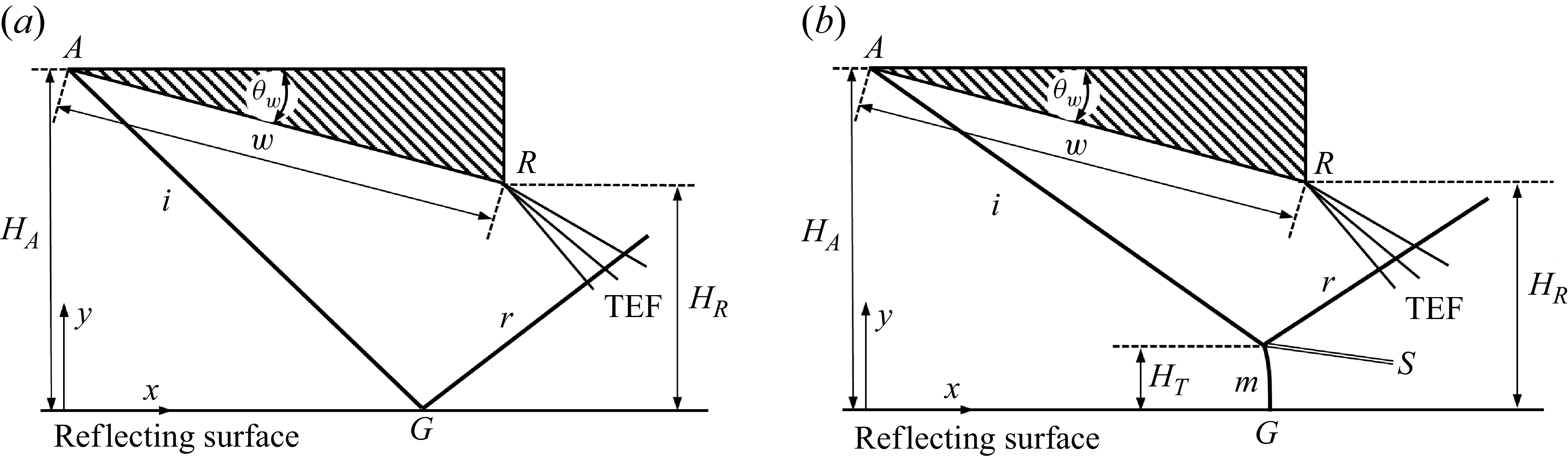
The reflection of an incident shock over a reflecting surface (symmetric line in the case of symmetric reflection), as shown in figure 1 for regular reflection (RR) and Mach reflection (MR), is an important phenomenon in steady supersonic flow. Whether RR or MR occurs depends not only on the inflow Mach number and the wedge angle, as described by the classical von Neumann and detachment conditions (von Neumann Reference von Neumann1943; Ben-Dor Reference Ben-Dor2007), but also on the geometric configuration, specifically on the relative height of the trailing edge.
Illustration of shock reflection for (a) RR, (b) MR, where TEF means trailing edge expansion fan.

Figure 1. Long description
Panel A: Diagram of regular reflection (RR). The reflecting surface is a symmetric line. The incident shock wave (i) reflects off the surface, creating a reflected shock wave (r). The trailing edge expansion fan (TEF) is also shown. Key points include A, G, and R, with heights HA and HR marked. Panel B: Diagram of Mach reflection (MR). Similar to Panel A, but includes an additional point S and a Mach stem (m). The incident shock wave (i) reflects off the surface, creating a reflected shock wave (r) and a transmitted shock wave (w). The trailing edge expansion fan (TEF) is also shown. Key points include A, G, and R, with heights HA, HR, and HT marked.
Studies in the 1970s led to controversial results about whether RR can exist in double solution. For instance, Henderson & Lozzi (Reference Henderson and Lozzi1975, Reference Henderson and Lozzi1979) and Hornung & Robinson (Reference Hornung and Robinson1982) failed to observe stable RR configurations inside the dual-solution domain. Though stability analysis showed that RR should be stable (Teshukov Reference Teshukov1989; Li & Ben-Dor Reference Li and Ben-Dor1996), and studies like those of Auld & Bird (Reference Auld and Bird1976) and Chpoun et al. (Reference Chpoun, Passerel, Li and Ben-Dor1995) successfully observed RR within a dual-solution domain, the previous controversial results have led to concerns about whether or how geometric set-up affects the shock reflection, according to Chpoun et al. (Reference Chpoun, Passerel, Li and Ben-Dor1995).
Hornung et al. (Reference Hornung, Oertel and Sandeman1979) introduced the ‘length scale’ concept in their study of the RR
 $\rightarrow$
MR transition, which implies that shock reflection depends on geometric set-up. Hornung & Robinson (Reference Hornung and Robinson1982) argued that the expansion fan from the trailing edge of the shock-generating wedge impinges the slipline from the triple point of MR and decreases the pressure along the slipline to match the pressure decrease in the quasi-one-dimensional flow duct formed between the slipline and the reflecting surface. The quasi-one-dimensional flow duct has a sonic throat upstream where the flow is subsonic. Hornung & Robinson (Reference Hornung and Robinson1982) further argued that the size and shape of this pocket are controlled by the distance between the Mach stem and the sonic throat, which in turn depends on the distance between the trailing edge of the wedge and the reflecting surface, so the Mach stem height follows
 \begin{align} \frac {H_{T}}{w}=f \!\left ( \gamma, M_{0},\theta _{w},\frac {H_{R}}{w}\right )\!, \end{align}
where
 $H_{T}$
is the Mach stem height,
 $w$
is the length of the lower wedge surface,
 $\gamma$
is the ratio of specific heats,
 $M_{0}$
is the inflow Mach number,
 $\theta _{w}$
is the wedge angle, and
 $H_{R}$
is the trailing edge height.
Chpoun et al. (Reference Chpoun, Passerel, Li and Ben-Dor1995) measured the effect of the geometrical set-up or length scale effect on the transition process for three different reflecting wedge surface lengths
 $w$
and three different inlet cross-sections (
 $H_{A}$
). The transition conditions displayed in the shock angle (incident shock)–shock angle (reflected shock) plane displayed differences for different geometric set-up. They concluded that the wave configuration within the dual-solution domain likely depends on geometrical parameters arising from both the experimental facility and the specific set-up.
To shed more light on and deepen the understanding of how the geometrical parameters affect the reflection process inside the dual-solution domain, Vuillon et al. (Reference Vuillon, Zeitoun and Ben-Dor1995) performed a systematic study of the geometric set-up on the shock reflection. They found that the distance
 $H_{R}$
is bounded by a lower limit (denoted
 $H_{R,\textit{min}})$
and an upper limit (
 $ H_{R,\textit{max}}$
), as shown in figure 2. The lower limit corresponds to the case in which the reflected shock wave grazes the trailing edge (
 $R$
). The upper limit is determined by the point where the leading characteristic of the trailing edge expansion fan intersects the incident shock wave at the reflection point (
 $G$
, see figure 1) for RR and at the triple point (
 $T$
) for MR.
Schematic illustration of MR for
 $H_{R}$
varying from
 $H_{R,\textit{min}}$
to
 $H_{R,\textit{max}}$
and beyond.

Vuillon et al. (Reference Vuillon, Zeitoun and Ben-Dor1995) stated the following.
-
(i) When
 $H_{R,\textit{min}}\lt H_{R}\lt H_{R,\textit{max}}$
, both RR and MR remain stable within the dual-solution domain.
-
(ii) When the distance
$H_{R}$
reaches or is reduced below
$H_{R,\textit{min}}$
, the MR becomes unstable and its Mach stem moves upstream until the MR vanishes and a bow shock wave is established ahead of the leading edge of the reflecting wedge. Under this condition, the flow will become subsonic, i.e. the flow is unstarted or chocked (a phenomenon also observed in numerical simulations and experiments by Chpoun et al. Reference Chpoun, Passerel, Li and Ben-Dor1995). -
(iii) Increasing
$H_{R}$
may trigger transition from MR to RR, and this transition occurs at
$H_{r}=H_{\textit{tr}}$
with
$H_{\textit{tr}}\lt H_{R,\textit{max}}$
.


Later, Li & Ben-Dor (Reference Li and Ben-Dor1997) corrected an error in the expression of Vuillon et al. (Reference Vuillon, Zeitoun and Ben-Dor1995) for
 $H_{R,\textit{max}}$
, and clarified that MR to RR transition occurs for
 $H_{R}\gt H_{R,\textit{max}}$
, i.e. beyond the threshold at which interaction between the trailing edge expansion fan and incident shock occurs. The expressions for
 $H_{R,\textit{min}}$
and
 $H_{R,\textit{max}}$
involve the Mach stem height
 $H_{T}$
. Vuillon et al. (Reference Vuillon, Zeitoun and Ben-Dor1995) suggested using the Mach stem height model of Azevedo & Liu (Reference Azevedo and Liu1993) to estimate
 $ H_{T}$
; Li & Ben-Dor (Reference Li and Ben-Dor1997) proposed their own model for
 $H_{R}$
. Grasso & Paoli (Reference Grasso and Paoli1999) studied the relaxation effect of non-equilibrium flow on
 $ H_{R,\textit{min}}$
and
 $H_{R,\textit{max}}$
, and concluded that relaxation reduces both
 $ H_{R,\textit{min}}$
and
 $H_{R,\textit{max}}$
.
Remarking that previous approximate Mach stem height models cannot predict accurate enough Mach stem height, Wang & Wu (Reference Wang and Wu2026) proposed a roadmap to find
 $H_{R,\textit{min}}$
for MR. However, in this roadmap, one has to find the linear coefficients involved in the Mach stem height expression using a set of high-fidelity numerical simulations based on computational fluid dynamics (CFD). This is expensive if we want to give this limit in the entire parameter space.
The MR for
 $H_{R}$
larger than
 $H_{R,\textit{max}}$
has been recently studied by Bai (Reference Bai2023), Baby et al. (Reference Baby, Paramanantham and Rajesh2024) and He & Shi (Reference He and Shi2025). Bai (Reference Bai2023) studied MR for
 $H_{R}$
larger than
 $H_{R,\textit{max}}$
, and determined the shock angle
 $\beta _{G}$
of the perturbed incident shock at the reflecting surface. The MR to RR transition condition occurs when
 $ \beta _{G}$
reaches its local von Neumann condition. For a given condition within the dual-solution domain, this transition condition was expressed as
 $ H_{R}=H_{\textit{tr}}$
(
 $\gt H_{R,\textit{max}}$
). Bai (Reference Bai2023) also updated a previous Mach stem height model to study how the Mach stem height decreases nonlinearly with
 $ H_{R}$
in the interval
 $H_{R,\textit{max}}\lt H_{R}\lt H_{\textit{tr}}$
.
The above-mentioned studies have revealed the importance of the parameters
 $ H_{R,\textit{min}}$
,
 $H_{R,\textit{max}}$
and
 $H_{\textit{tr}}$
. However, for MR, both
 $H_{R,\textit{min}}$
and
 $H_{R,\textit{max}}$
involve the Mach stem height
 $H_{T}$
. When an approximate Mach stem height model is used, the accuracy is poor, as demonstrated by Wang & Wu (2026) for
 $H_{R,\textit{min}}$
using the approximate model of Bai & Wu (Reference Bai and Wu2021). When CFD is used, producing the limits in the entire parameter space is expensive.
Thus to have quantitative information about the geometric limits
 $H_{R,\textit{min}}$
and
 $H_{R,\textit{max}}$
, the obstacle is the lack of an accurate enough Mach stem height model. Mach stem height models involve several submodels, including the triple-point model, the slipline model and the reflected shock/expansion fan interaction model. Excellent studies have been carried out to advance the various submodels and the global algorithm for the physics of Mach stem height modelling (e.g. Azevedo & Liu Reference Azevedo and Liu1993; Li & Ben-Dor Reference Li and Ben-Dor1997; Mouton & Hornung Reference Mouton and Hornung2007; Gao & Wu Reference Gao and Wu2010; Bai & Wu Reference Bai and Wu2017, Reference Bai and Wu2021; Shoesmith & Timofeev Reference Shoesmith and Timofeev2021; Bai Reference Bai2023; Chernyshov & Savelova Reference Chernyshov and Savelova2023). See Li & Bai (Reference Li and Bai2026) for more references.
Li & Bai (Reference Li and Bai2026) conducted a study of the performance of various submodels, and concluded that using compatibility relations in the interactive part of the slipline is superior to the wave reflection model and better captures the linear slope of Mach stem height with wedge trailing edge height. Nevertheless, despite various improvements, prediction errors in the slope and systematic biases in the overall Mach stem height prediction persist. To address these shortcomings, they developed a calibrated scaling law for the coefficient of a linear Mach stem model. Their calibrated scaling law is grounded in asymptotic reasoning and high-fidelity numerical simulations.
In the following, we will use the relative trailing edge height
 $g={H_{R} }/{H_{A}}$
and the relative lower limit
 $g_{\textit{min}}= {H_{R,\textit{min}}}/{H_{A}}$
and upper limit
 $g_{\textit{max}}= {H_{R,\textit{max}}}/{H_{A}}$
.
In the present paper, we derive algebraic expressions for
 $g_{\textit{min}}$
and
 $g_{\textit{max}}$
for MR, where the Mach stem height is evaluated using the calibrated model of Li & Bai (Reference Li and Bai2026). We then consider all limits along the entire
 $g$
-axis, and study the gaps between various limits. The present study focuses on inviscid two-dimensional flow without considering real-gas effects (e.g. high-temperature effects at large Mach numbers). See Wang & Wu (2026) for a discussion of how to account for the effect of boundary layer along the wedge surface.
The algebraic expressions for the estimation of
 $g_{\textit{min}}$
and
 $g_{\textit{max}}$
, with the Mach stem height estimated by the calibrated model of Li & Bai (Reference Li and Bai2026), are derived in § 2. Quantitative studies are provided in § 3 for
 $g_{\textit{min}}$
and for the dual-solution stability gap. The results are displayed in the
 $M_{0}{-}\theta _{w}$
space. Comparison between the present algebraic model and previous CFD data and models is given, showing how accurate is the algebraic model. The dependence of
 $g_{\textit{min}}$
for both MR and RR and the dual-solution stability gap on
 $M_{0}$
and
 $ \theta _{w}$
is discussed. Similar quantitative studies are done for
 $ g_{\textit{max}}$
, and the details are provided in § 4. Section 5 is devoted to all possible limits and gaps along the
 $g$
-axis. The lower limits
 $ g_{\textit{min}}$
for both RR and MR, the upper limits
 $g_{\textit{max}}$
for both RR and MR, and the MR to RR transition limit
 $g_{\textit{tr}}=H_{\textit{tr}}/H_{A}$
are the five limits with clear physical meanings. The gaps between the ends of the
 $g$
-axis and various limits define various types of shock reflection. We will also consider whether these limits and the gaps between these limits are exclusive. Concluding remarks are provided in § 6.
2. Method for predicting the lower and upper limits
2.1. Implicit forms for
$g_{\textit{min}}$
and
$g_{\textit{max}}$


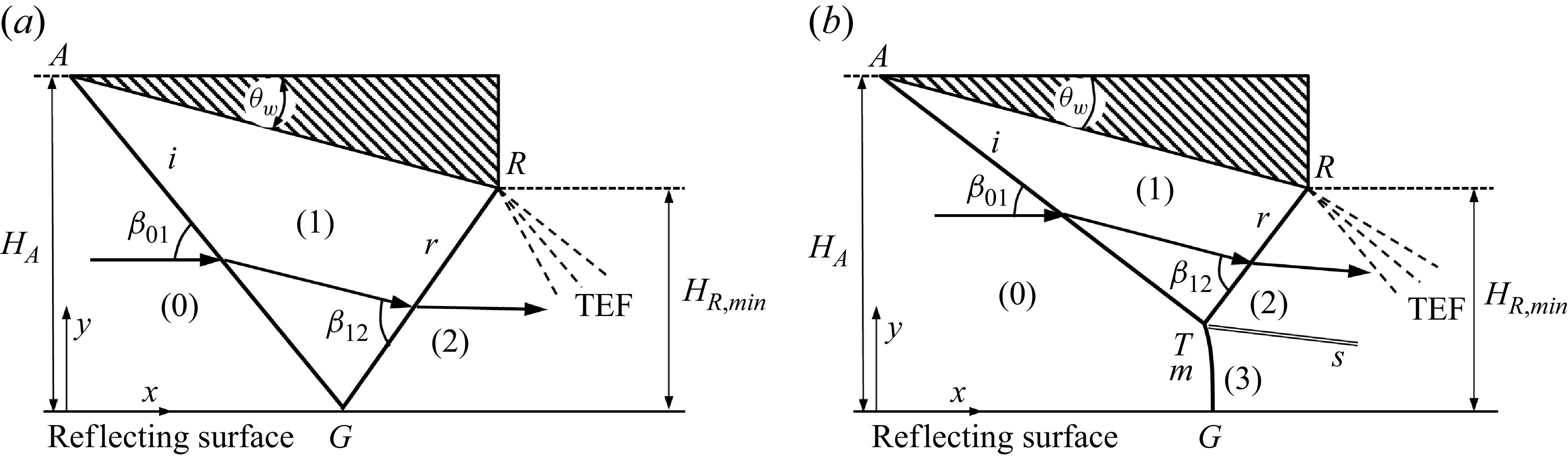
Following Vuillon et al. (Reference Vuillon, Zeitoun and Ben-Dor1995), the geometrical set-up for
 $ H_{R}=H_{R,\textit{min}}$
is shown schematically in figure 3. Here,
 $\beta _{01}$
is the shock angle of the incident shock (
 $i$
), and
 $\beta _{12}$
is the shock angle of the reflected shock (in the vicinity of the triple point for MR or of the reflection point for RR). Li & Ben-Dor (Reference Li and Ben-Dor1997) gave
 \begin{align} H_{R,\textit{min}}=H_{T}+\phi w, \end{align}
where
 \begin{align} \phi =\frac {\sin (\beta _{12}-\theta _{w})\sin (\beta _{01}-\theta _{w})}{ \sin (\beta _{01}+\beta _{12}-\theta _{w})}. \end{align}
Illustration of shock reflection at
 $H_{R}=H_{R,\textit{min}}$
for (a) RR, (b) MR.

Figure 3. Long description
Panel A: Diagram of regular reflection (RR) in supersonic flow. The reflecting surface is labeled G, and the incident shock wave is labeled i. The reflected shock wave is labeled R, and the Mach stem is labeled r. The angles beta 01 and beta 12 are indicated, along with the regions labeled 0, 1, and 2. The trailing edge flux (TEF) is marked on the right side. The height from the reflecting surface to the top of the incident shock wave is labeled H A, and the minimum height from the reflecting surface to the top of the reflected shock wave is labeled H R,min. Panel B: Diagram of Mach reflection (MR) in supersonic flow. The reflecting surface is labeled G, and the incident shock wave is labeled i. The reflected shock wave is labeled R, and the Mach stem is labeled r. The angles beta 01 and beta 12 are indicated, along with the regions labeled 0, 1, 2, and 3. The triple point is labeled T m, and the slipstream is labeled s. The trailing edge flux (TEF) is marked on the right side. The height from the reflecting surface to the top of the incident shock wave is labeled H A, and the minimum height from the reflecting surface to the top of the reflected shock wave is labeled H R,min.
Wang & Wu (2026) replaced (2.1) by
 \begin{align} H_{R,\textit{min}}=H_{T,min }+\phi w_{\textit{min}}, \end{align}
where
 $H_{T,min }$
and
 $w_{\textit{min}}$
are values at
 $H_{R}=H_{R,\textit{min}}$
. Here,
 \begin{align} w_{\textit{min}}=\frac {H_{A}-H_{R,\textit{min}}}{\sin \theta _{w}}=\frac {1-g_{\textit{min}}}{\sin \theta _{w}}H_{A}, \end{align}
and
 $H_{T,min }$
satisfies the functional form (1.1), i.e.
 ${ H_{T,min }}/{w}=f ( M_{0},\theta _{w},\gamma, ( {H_{R,\textit{min}}}/{w}) )$
or
 \begin{align} \frac {H_{T,min }}{H_{A}}=f\left ( M_{0},\theta _{w},\gamma, \frac {H_{R,\textit{min}} }{H_{A}}\right ). \end{align}
Putting (2.4) and (2.5) into (2.3), and using
 $ g_{\textit{min}}$
for
 ${H_{R,\textit{min}}}/{H_{A}}$
, Wang & Wu (2026) obtained
 \begin{align} g_{\textit{min}}=f\left ( M_{0},\theta _{w},\gamma, g_{\textit{min}}\right ) +\frac {\phi }{ \sin \theta _{w}}\left ( 1-g_{\textit{min}}\right ). \end{align}
Now consider
 $H_{R,\textit{max}}$
. Following Vuillon et al. (Reference Vuillon, Zeitoun and Ben-Dor1995), the geometrical set-up for
 $H_{R}=H_{R,\textit{max}}$
is shown schematically in figure 4. Here,
 $\mu _{1}=\arcsin( {1}/{M_{1}})$
is the Mach angle of the leading characteristics of the trailing edge expansion fan. Originally, Li & Ben-Dor (Reference Li and Ben-Dor1997) gave
 \begin{align} H_{R,\textit{max}}=H_{T}+\psi w, \end{align}
where
 \begin{align} \psi =\frac {\sin (\mu _{1}+\theta _{w})\sin (\beta _{01}-\theta _{w})}{\sin (\mu _{1}+\theta _{w}-\beta _{01})}. \end{align}
Illustration of shock reflection at
 $H_{R}=H_{R,\textit{max}}$
for (a) RR, (b) MR.

Following the procedure of Wang & Wu (2026) for
 $H_{R,\textit{min}}$
, for
 $ H_{R,\textit{max}}$
we replace (2.7) by
 \begin{align} H_{R,\textit{max}}=H_{T,max }+\psi w_{\textit{max}}, \end{align}
which can be rewritten as
 \begin{align} g_{\textit{max}}=f \!\left ( M_{0},\theta _{w},\gamma, g_{\textit{max}}\right ) +\frac {\psi }{ \sin \theta _{w}}\left ( 1-g_{\textit{max}}\right ) \end{align}
when the three expressions
 \begin{align} w_{\textit{max}}=\frac {H_{A}-H_{R,\textit{max}}}{\sin \theta _{w}}, \end{align}
 \begin{align} \frac {H_{T,max }}{H_{A}}=f \!\left ( M_{0},\theta _{w},\gamma, \frac {H_{R,\textit{max}} }{H_{A}}\right ) \end{align}
and
 $g_{\textit{max}}={H_{R,\textit{max}}}/{H_{A}}$
are used.
2.2. Explicit expressions for
$g_{\textit{min}}$
and
$g_{\textit{max}}$


Previous studies about Mach stem height explicitly or implicitly assume that (1.1) can be well represented by the linear form (see Li & Bai Reference Li and Bai2026)
 \begin{align} \frac {H_{T}}{H_{A}}=A\frac {H_{R}}{H_{A}}+B, \end{align}
where
 $A=A(M_{0},\theta _{w})$
and
 $B=B(M_{0},\theta _{w})$
. Wang & Wu (2026) showed that if the linear form (2.13) is used so that
 $ {H_{T,min }}/{H_{A}}=A( {H_{R,\textit{min}}}/{H_{A}})+B$
, then the expression (2.6) takes the explicit form
 \begin{align} g_{\textit{min}}=\frac {\frac{\phi }{\sin \theta _{w}}+B}{1-A+\frac{\phi}{\sin \theta _{w}}}. \end{align}
Here, we follow the same approach for
 $g_{\textit{max}}$
, and write
 $ {H_{T,max } }/{H_{A}}=A( {H_{R,\textit{max}}}/{H_{A}})+B$
and write the expression (2.10) as the explicit form
 \begin{align} g_{\textit{max}}=\frac {\frac{\psi }{\sin \theta _{w}}+B}{1-A+\frac{\psi }{\sin \theta _{w}}}. \end{align}
The linear expression (2.13) may be less accurate for small
 $M_{0}$
and for
 $\theta _{w}$
approaching the von Neumann condition (Li & Bai Reference Li and Bai2026). To increase the accuracy, one possible way is to replace (2.13) by the more accurate second-order form
 \begin{align} \frac {H_{T}}{H_{A}}=A\frac {H_{R}}{H_{A}}+C\left ( \frac {H_{R}}{H_{A}}\right ) ^{2}+B, \end{align}
so (2.14) becomes
 \begin{align} g_{\textit{min}}=\frac {\alpha _{1}-\sqrt {\alpha _{1}^{2}-4C\alpha _{2}}}{2C}, \end{align}
where
 $\alpha _{1}=1-A+({\phi }/{\sin \theta _{w}})$
and
 $\alpha _{2}=B+ ( {\phi }/{\sin \theta _{w}})$
, and (2.15) becomes
 \begin{align} g_{\textit{max}}=\frac {\alpha _{3}-\sqrt {\alpha _{3}^{2}-4C\alpha _{4}}}{2C}, \end{align}
where
 $\alpha _{3}=1-A+( {\psi }/{\sin \theta _{w}})$
and
 $\alpha _{4}=B+({\psi }/{\sin \theta _{w}})$
.
Here, we only use the linear form since we only have a formula of Mach stem height within the range of linear variation.
There are a number of studies for the prediction of Mach stem height for
 $ g_{\textit{min}}\lt g\lt g_{\textit{max}}$
(e.g. Azevedo & Liu Reference Azevedo and Liu1993; Li & Ben-Dor Reference Li and Ben-Dor1997; Schotz et al. Reference Schotz, Levy, Ben-Dor and Igra1997; Mouton & Hornung Reference Mouton and Hornung2007; Gao & Wu Reference Gao and Wu2010; Bai & Wu Reference Bai and Wu2017, Reference Bai and Wu2021; Shoesmith & Timofeev Reference Shoesmith and Timofeev2021; Bai Reference Bai2023; Chernyshov & Savelova Reference Chernyshov and Savelova2023). Recently, Mach stem height models have also been studied for
 $g\lt g_{\textit{max}}$
(Bai Reference Bai2023; He & Shi Reference He and Shi2025). These Mach stem height models are all approximate. Wang & Wu (2026) used the approximate model of Bai & Wu (Reference Bai and Wu2021) to compute
 $A$
and
 $B$
required in (2.14), and showed that the relative error between predicted
 $g_{\textit{min}}$
and CFD-based
 $g_{\textit{min}}$
can be larger than 50 %.
Li & Bai (Reference Li and Bai2026) performed a study about the accuracy of various submodels in Mach stem height modelling, and concluded that the prediction is highly sensitive to submodels of slipline and reflected shock. In all cases, quantitatively exact modelling is impossible. They thus proposed a calibrated formula for
 $A$
and
 $B$
fitted from a finite number numerical simulations, for
 $\gamma =1.4$
. The fitted formulas are found to predict Mach stem heights with relative error smaller than
 $10\,\%$
for a wide parameter space. Their calibrated formulas to compute
 $A$
and
 $B$
are
 \begin{align} A=0.59M_{0}^{0.14}\,{\rm e}^{-0.15M_{0}+2.25}\ln \frac {\theta _{\textit{max}}(M_{0})-\theta _{w}}{\theta _{\textit{max}}(M_{0})-\theta ^{(N)}(M_{0})} \end{align}
and
 \begin{align} B=-1.31M_{0}^{-0.31}\,{\rm e}^{-0.10M_{0}+1.53}\ln \frac {\theta _{\textit{max}}(M_{0})-\theta _{w}}{\theta _{\textit{max}}(M_{0})-\theta ^{(N)}(M_{0})}, \end{align}
where
 $\theta ^{(N)}$
is the von Neumann condition, and
 $\theta _{\textit{max}}$
is the detached angle of the incident shock.
3. A study of the lower limits for RR and MR
The lower limits will be given in the
 $M_{0}{-}\theta _{w}$
plane with
 $ 2.3\lt M_{0}\lt 7$
. Real gas effect is not considered in this paper for large enough Mach number, so we take
 $\gamma =1.4$
. Note that
 $M_{0}=2.3$
is close to the left-hand corner of the dual-solution domain, where
 $\theta _{w}^{(D)}$
is very close to
 $\theta _{w}^{(N)}$
, so we do not display the results for
 $ M_{0}\leqslant 2.3$
.
3.1. Lower limit
$g_{\textit{min}}^{(\textit{RR})}$
in the
$M_{0}{-}\theta _{w}$
plane


The lower limit for RR, denoted
 $g_{\textit{min}}^{(\textit{RR})}$
, is obtained by (2.14) with
 $A=B= 0$
and with
 $\phi$
computed by (2.2), where
 $\beta _{12}$
is the shock angle of the reflected shock for RR. Note that the expression for
 $g_{\textit{min}}^{(\textit{RR})}$
is exact and is displayed by Wang & Wu (2026) within the dual-solution domain. Here, in figure 5, we display
 $g_{\textit{min}}^{(\textit{RR})}$
in the entire space
 $0\lt \theta _{w}\lt \theta _{w}^{(D)}$
, where
 $\theta _{w}^{(D)}=\theta _{w}^{(D)}(M_{0})$
is the detachment condition.
Contour lines (solid) of
 $g_{\textit{min}}^{(\textit{RR})}$
in the
 $M_{0}{-}\theta _{w}$
plane. Dashed lines represent critical conditions.

It is seen that for
 $\theta _{w}\rightarrow 0$
,
 $g_{\textit{min}}^{(\textit{RR})}$
approaches
 $1$
, meaning that for very weak shock waves (for
 $\theta _{w}\rightarrow 0$
), RR can occur for all
 $g$
and for all
 $M_{0}$
with
 $ 2.3\lt M_{0}\lt 7$
. When
 $\theta _{w}$
increases for fixed
 $M_{0}$
, the lower limit
 $g_{\textit{min}}^{(\textit{RR})}$
first decreases then increases, and the minimum value of
 $g_{\textit{min}}^{(\textit{RR})}$
occurs at
 $\theta_w=\theta _{w,m}$
, where
 $ \theta _{w,m}=\theta _{w,m}(M_{0})$
is the value of
 $\theta _{w}$
at which
 \begin{align} \frac {\partial g_{\textit{min}}^{(\textit{RR})}(M_{0},\theta _{w})}{\partial \theta _{w}}=0. \end{align}
For convenience, the critical line
 $\theta _{w}=\theta _{w,m}(M_{0})$
will be called the dividing line for monotonicity. As shown in figure 5, there is a point, denoted
 $P$
, with
 $M_{0}=M_{P}\approx 3.25$
; when
 $ M_{0}\lt M_{P}$
, the dividing line for monotonicity is below the von Neumann condition
 $\theta _{w}^{(N)}=\theta _{w}^{(N)}(M_{0})$
, while for
 $ M_{0}\gt M_{P}$
, the dividing line for monotonicity is above the von Neumann condition
 $\theta _{w}^{(N)}=\theta _{w}^{(N)}(M_{0})$
.
3.2. Lower limit
$g_{\textit{min}}^{(\textit{MR})}$
in the
$M_{0}{-}\theta _{w}$
plane


The lower limit for MR, denoted
 $g_{\textit{min}}^{(\textit{MR})}$
, is obtained by (2.14), with
 $A$
and
 $B$
given by the calibrated formulas (2.19) and (2.20), respectively. The quantity
 $\phi$
is computed by (2.2), where the
 $\beta _{12}$
is the shock angle of the reflected shock that is given by the triple-point solution.
Figure 6 displays
 $g_{\textit{min}}^{(\textit{MR})}$
in the
 $M_{0}{-}\theta _{w}$
plane, for
 $\theta _{w}^{(N)}\lt \theta _{w}\lt \theta _{\textit{max}}$
, where
 $\theta _{\textit{max}}=\theta _{\textit{max}}(M_{0})$
is the detached angle for incident shock. Unlike
 $g_{\textit{min}}^{(\textit{RR})}$
, which varies non-monotonically for increasing
 $ \theta _{w}$
, here
 $g_{\textit{min}}^{(\textit{MR})}$
increases monotonically with
 $\theta _{w}$
when
 $\theta _{w}$
varies from
 $\theta _{w}^{(N)}$
to
 $\theta _{w}^{(D)}$
.
Contour lines (solid) of
 $g_{\textit{min}}^{(\textit{MR})}$
in the
 $M_{0}{-}\theta _{w}$
plane. Dashed lines represent critical conditions.

Figure 6. Long description
A line graph with contour lines and critical conditions. The horizontal axis is labeled M 0 ranging from 2.5 to 7.0. The vertical axis is labeled theta w in degrees ranging from 15 to 40. Solid lines represent contour lines with values 0.16, 0.21, 0.26, 0.31, 0.36, 0.41, 0.46, 0.51, 0.56, 0.61, 0.66, 0.71, and 0.76. Dashed lines represent critical conditions labeled theta w max, theta w D, and theta w N. The contour lines show an increasing trend as M 0 increases.
At fixed Mach number, the value of
 $g_{\textit{min}}^{(\textit{MR})}$
is larger for larger wedge angle. For instance, at
 $M_{0}=4$
, we have
 $g_{\textit{min}}^{(\textit{MR})}\approx 0.23$
for
 $\theta _{w}\rightarrow \theta _{w}^{(N)}$
and
 $g_{\textit{min}}^{(\textit{MR})}\approx 0.69$
for
 $\theta _{w}\rightarrow \theta _{\textit{max}}$
. At fixed wedge angle, the value of
 $g_{\textit{min}}^{(\textit{MR})}$
is larger for smaller Mach number.
High-fidelity CFD data are used by Wang & Wu (2026) to assess the correctness of the semi-empirical roadmap to determine
 $ g_{\textit{min}}^{(\textit{MR})}$
. These data are used here to assess the accuracy of (2.14), with
 $A$
and
 $B$
given by the calibrated formulas (2.19) and (2.20), respectively.
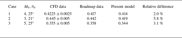
Table 1 gives three cases for which the present algebraic model defined by (2.14), (2.19) and (2.20) is compared with the CFD data and semi-empirical roadmap data of Wang & Wu (2026). The relative difference between the present algebraic model and the CFD data is below 6 % for all cases.
A comparison of
 $g_{\textit{min}}$
from different estimations. Here, CFD data are
 $g_{min}$
by CFD of Wang & Wu (2026), roadmap data are
 $g_{min}$
by the roadmap of Wang & Wu (2026), and the present model is
 $g_{min}$
by (2.14), (2.19) and (2.20).

Table 1. Long description
A table comparing different estimation models for three cases. The table has five columns: Case, M 0, θ w, CFD data, Roadmap data, Present model, and Relative difference. It has three rows of data. Row 1: Case 1, M 0, θ w 4, 25 degrees, CFD data 0.4225 ± 0.0025, Roadmap data 0.417, Present model 0.414, Relative difference 2.0 percent. Row 2: Case 2, M 0, θ w 3, 21 degrees, CFD data 0.445 ± 0.005, Roadmap data 0.442, Present model 0.419, Relative difference 5.8 percent. Row 3: Case 3, M 0, θ w 5, 25 degrees, CFD data 0.355 ± 0.005, Roadmap data 0.358, Present model 0.344, Relative difference 3.1 percent.
3.3. The dual-solution stability gap
$g_{\textit{min}}^{(\textit{MR})}-g_{\textit{min}}^{(\textit{RR})}$
in the
$M_{0}{-}\theta _{w}$
plane


The dual-solution stability gap (Wang & Wu 2026) is computed by
 \begin{align} \Delta g_{\textit{min}}=g_{\textit{min}}^{(\textit{MR})}-g_{\textit{min}}^{(\textit{RR})}, \end{align}
where
 $g_{\textit{min}}^{(\textit{RR})}$
is given in § 3.1, and
 $g_{\textit{min}}^{(\textit{MR})}$
is given in § 3.2. Note that
 $g_{\textit{min}}^{(\textit{RR})}$
is defined for
 $\theta _{w}\lt \theta _{w}^{(D)}$
, and
 $g_{\textit{min}}^{(\textit{MR})}$
is defined for
 $\theta _{w}\gt \theta _{w}^{(N)}$
, so
 $\Delta g_{\textit{min}}$
is defined in the dual-solution domain
 $\theta _{w}^{(N)}\lt \theta _{w}\lt \theta _{w}^{(D)}$
.
Figure 7 displays
 $\Delta g_{\textit{min}}=g_{\textit{min}}^{(\textit{MR})}-g_{\textit{min}}^{(\textit{RR})}$
, in the dual-solution domain. For
 $\theta _{w}\rightarrow \theta _{w}^{(N)}$
, we have
 $\Delta g_{\textit{min}}\rightarrow 0$
, meaning that there is no dual-solution stability gap for
 $\theta _{w}$
approaching the von Neumann condition.
Contour lines (solid) of
 $\Delta g_{\textit{min}}=g_{\textit{min}}^{(\textit{MR})}-g_{\textit{min}}^{(\textit{RR})}$
in the dual-solution domain plane. Dashed lines represent critical conditions.

Figure 7. Long description
A line graph with contour lines and critical conditions in a dual-solution domain plane. The horizontal axis is labeled M 0 and ranges from 2.5 to 7.0. The vertical axis is labeled theta w in degrees and ranges from 16 to 30. Solid contour lines are labeled with values ranging from 0.02 to 0.22. Dashed lines represent critical conditions. A closed curve is indicated at the top right, with a maximum point Q marked. The graph shows a vanishing point and trends of increasing and decreasing values.
It is interesting to note that there exists a maximum point for
 $\Delta g_{\textit{min}}$
within the dual-solution domain. This maximum point, denoted
 $Q$
in figure 7, lies at
 \begin{align} M_{0}\approx 6.2,\quad\theta _{w}\approx 28.8^\circ, \end{align}
and the maximal value of
 $\Delta g_{\textit{min}}$
is
 \begin{align} {\rm max} (\Delta g_{\textit{min}})=0.225\text{.} \end{align}
The contour lines with constant
 $\Delta g_{\textit{min}}$
form closed curves enclosing point
 $Q$
. The existence of this maximum point means that the range of
 $g$
with stable dual solution is the largest there.
Similarly as for
 $g_{\textit{min}}^{(\textit{RR})}$
, for which there is a dividing line for monotonicity (figure 5), here there is also a dividing line for monotonicity (marked by black circles in figure 7). Since
 $ g_{\textit{min}}^{(\textit{MR})}$
is monotonic according to figure 6, the non-monotonicity of
 $\Delta g_{\textit{min}}=g_{\textit{min}}^{(\textit{MR})}-g_{\textit{min}}^{(\textit{RR})}$
follows naturally from the non-monotonicity of
 $g_{\textit{min}}^{(\textit{RR})}$
.
Wang & Wu (2026) have given a formal proof of
 $\Delta g_{\textit{min}}\gt 0$
except near the left tip-horn region of the dual-solution domain. Using the approximate Mach stem height model of Bai & Wu (Reference Bai and Wu2021), this tip-horn region still exists according to Wang & Wu (2026, figure 13). Here, by using the calibrated Mach stem height model, we have
 $\Delta g_{\textit{min}}\gt 0$
in the entire dual-solution domain (except
 $\theta _{w}\rightarrow \theta _{w}^{(N)}$
).
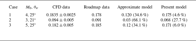
To assess the accuracy, we still consider the three cases shown in table 1. The comparison is given in table 2, where we also give an estimation using an approximate Mach stem height model in the expression (2.14) for
 $g_{\textit{min}}^{(\textit{MR})}$
. It is seen that for cases 1 and 3, the present model compares well with CFD data, but for case 2, the error is relatively large (this is probably because the absolute value of
 $\Delta g_{\textit{min}}$
is small). For an approximate Mach stem height model, the relative errors are large for all three cases.
A comparison of
 $\Delta g_{\textit{min}}$
from different estimations. Approximate model is the model using the Mach stem height model of Bai & Wu (Reference Bai and Wu2021); see Appendix A of Wang & Wu (2026).

Table 2. Long description
A table comparing different estimation models for three cases. The table has five columns: Case, CFD data, Roadmap data, Approximate model, and Present model. It has three rows with different cases. Row 1: Case 1, M 0, 4, theta w, 25 degrees, CFD data, 0.1835 plus or minus 0.0025, Roadmap data, 0.178, Approximate model, 0.120, 34.6 percent, Present model, 0.175, 4.6 percent. Row 2: Case 2, M 0, 3, theta w, 21 degrees, CFD data, 0.094 plus or minus 0.005, Roadmap data, 0.091, Approximate model, 0.03, 68.1 percent, Present model, 0.068, 27.7 percent. Row 3: Case 3, M 0, 5, theta w, 25 degrees, CFD data, 0.182 plus or minus 0.005, Roadmap data, 0.185, Approximate model, 0.12, 34.1 percent, Present model, 0.171, 6.0 percent.
4. A study of upper limits for RR and MR
As for the lower limits, the upper limits will be given in the
 $M_{0}{-}\theta _{w}$
plane with
 $2.3\lt M_{0}\lt 7$
, and real gas effect is not considered for large enough Mach number, so we take
 $\gamma =1.4$
.
4.1. Upper limit
$g_{\textit{max}}^{(\textit{RR})}$
in the
$M_{0}{-}\theta _{w}$
plane


The upper limit for RR, denoted
 $g_{\textit{max}}^{(\textit{RR})}$
, is obtained by (2.15) with
 $A=B= 0$
and with
 $\psi$
computed by (2.8). Note that the expression for
 $g_{\textit{max}}^{(\textit{RR})}$
is exact and has already been displayed by Bai (Reference Bai2023). Here, for the purpose of comparing with lower limit behaviour, in figure 8, we display
 $ g_{\textit{min}}^{(\textit{RR})}$
in the space
 $0\lt \theta _{w}\lt \theta _{w}^{(D)}$
, where
 $ \theta _{w}^{(D)}=\theta _{w}^{(D)}(M_{0})$
is the detachment condition.
Contour lines (solid) of
 $g_{\textit{max}}^{(\textit{RR})}$
in the
 $M_{0}{-}\theta _{w}$
plane. Dashed lines represent critical conditions.

Unlike
 $g_{\textit{min}}^{(\textit{RR})}$
, which varies non-monotonically for increasing
 $ \theta _{w}$
, here
 $g_{\textit{max}}^{(\textit{RR})}$
increases monotonically with
 $\theta _{w}$
when
 $\theta _{w}$
varies from
 $\theta _{w}^{(D)}$
to
 $0$
. Similarly as
 $g_{\textit{min}}^{(\textit{RR})}$
, for
 $\theta _{w}\rightarrow 0$
and for all
 $M_{0}$
with
 $2.3\lt M_{0}\lt 7$
,
 $g_{\textit{max}}^{(\textit{RR})}$
approaches
 $1$
, meaning that for very weak shock waves (for
 $\theta _{w}\rightarrow 0$
), RR without interference can occur for all
 $g$
.
4.2. Upper limit
$g_{\textit{max}}^{(\textit{MR})}$
in the
$M_{0}{-}\theta _{w}$
plane


The upper limit for MR, denoted
 $g_{\textit{max}}^{(\textit{MR})}$
, is obtained by (2.15) with
 $A$
and
 $B$
given by the calibrated formulas (2.19) and (2.20), respectively, and with
 $\psi$
computed by (2.8).
Figure 9 displays
 $g_{\textit{max}}^{(\textit{MR})}$
in the
 $M_{0}{-}\theta _{w}$
plane. The behaviour of
 $g_{\textit{max}}^{(\textit{MR})}$
is much like
 $g_{\textit{min}}^{(\textit{RR})}$
, the lower limit for RR, in the dual-solution domain. When
 $\theta _{w}$
increases for fixed
 $M_{0}$
, the upper limit
 $g_{\textit{max}}^{(\textit{MR})}$
first decreases then increases, and the minimum value of
 $g_{\textit{max}}^{(\textit{MR})}$
occurs at
 $\theta_w=\theta _{w,m}$
, where
 $\theta _{w,m}=\theta _{w,m}(M_{0})$
is the value of
 $\theta _{w}$
at which
 \begin{align} \frac {\partial g_{\textit{max}}^{(\textit{MR})}(M_{0},\theta _{w})}{\partial \theta _{w}}=0. \end{align}
For convenience, the critical line
 $\theta _{w}=\theta _{w,m}(M_{0})$
will be called the dividing line for monotonicity (marked with black circles). As shown in figure 9, there is a point, denoted
 $P$
, with
 $ M_{0}=M_{P}\approx 5.4$
; when
 $M_{0}\lt M_{P}$
, the dividing line for monotonicity is below the detachment condition
 $\theta _{w}^{(D)}=\theta _{w}^{(D)}(M_{0})$
, while for
 $M_{0}\gt M_{P}$
, the dividing line for monotonicity is above the detachment condition
 $\theta _{w}^{(D)}=\theta _{w}^{(D)}(M_{0})$
.
Contour lines (solid) of
 $g_{\textit{max}}^{(\textit{MR})}$
in the
 $M_{0}{-}\theta _{w}$
plane. Dashed lines represent critical conditions.

Figure 9. Long description
A line graph with contour lines (solid) and critical conditions (dashed lines) in the plane. The horizontal axis is labeled M 0 and ranges from 2.5 to 7.0. The vertical axis is labeled theta w (degrees) and ranges from 15 to 40 degrees. The contour lines are labeled with values ranging from 0.6 to 0.775. The dashed lines represent critical conditions, including theta max, theta w (D), and theta w (N). The graph shows an increase in theta w as M 0 increases, with specific points marked and labeled.
4.3. Dual-solution interference gap
$g_{\textit{max}}^{(\textit{MR})}-g_{\textit{max}}^{(\textit{RR})}$
in the
$M_{0}{-}\theta _{w}$
plane


The dual-solution interference gap
 $\Delta g_{\textit{max}}$
is the difference between
 $g_{\textit{max}}^{(\textit{MR})}$
and
 $g_{\textit{max}}^{(\textit{RR})}$
, i.e.
 \begin{align} \Delta g_{\textit{max}}=g_{\textit{max}}^{(\textit{MR})}-g_{\textit{max}}^{(\textit{RR})}\text{.} \end{align}
This gap is defined in the dual-solution domain since
 $g_{\textit{max}}^{(\textit{MR})}$
exists for
 $\theta _{w}\lt \theta _{w}^{(D)}$
, and
 $g_{\textit{max}}^{(\textit{RR})}$
exists for
 $\theta _{w}\gt \theta _{w}^{(N)}$
.
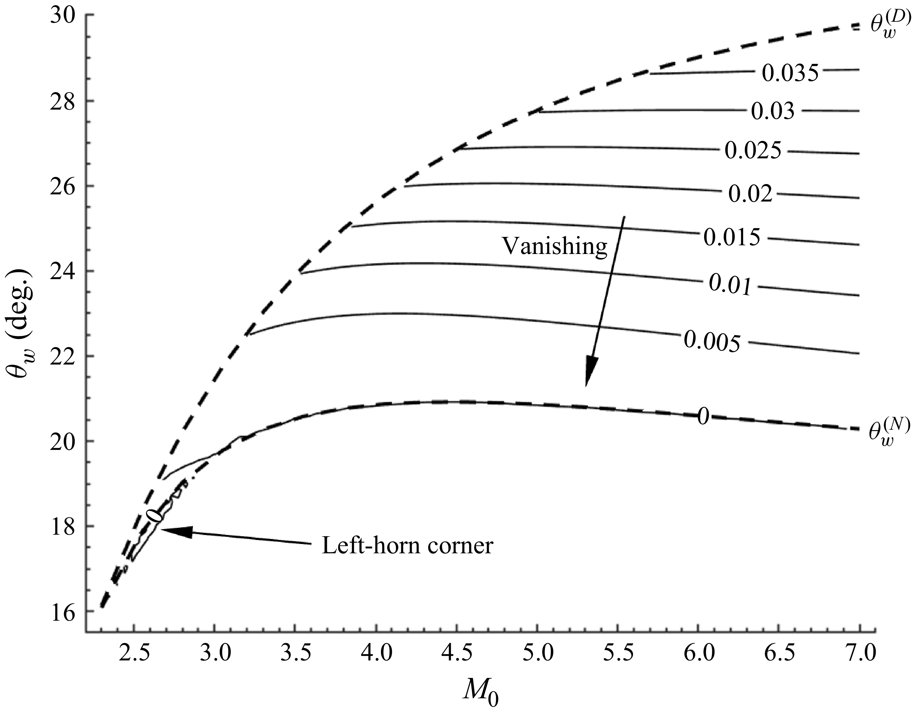
Figure 10 displays
 $\Delta g_{\textit{max}}$
in the dual-solution domain. The contour lines are almost horizontal lines, so
 $\Delta g_{\textit{max}}$
is insensitive to the Mach number.
Similarly as for
 $\Delta g_{\textit{min}}$
(figure 7),
 $\Delta g_{\textit{max}}$
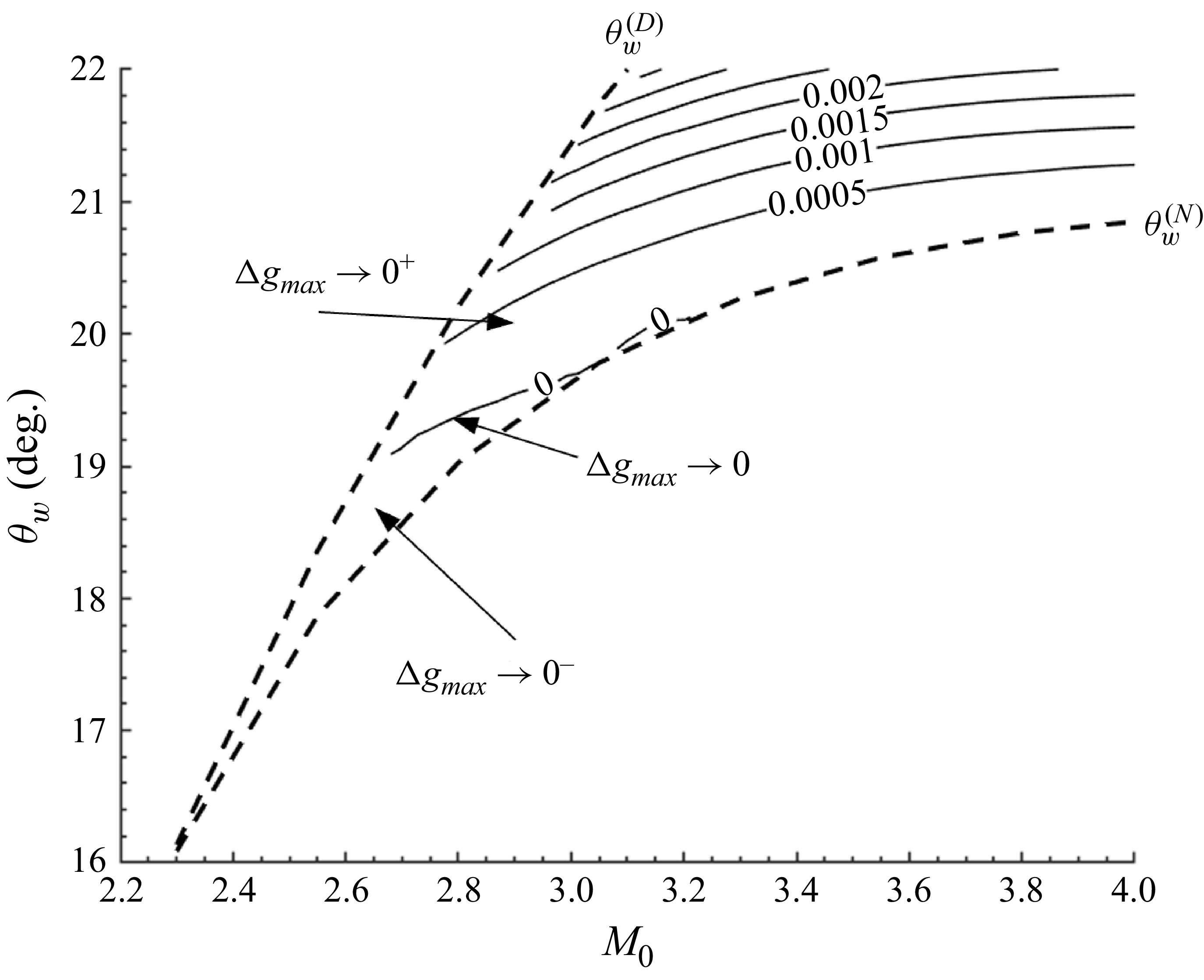
is small at the left-horn corner of the dual-solution domain. Note that
 $ \Delta g_{\textit{max}}$
may display very small negative values due to rounding errors (figure 11). For
 $\theta _{w}\rightarrow \theta _{w}^{(N)}$
, we have
 $\Delta g_{\textit{max}}\rightarrow 0$
, meaning that there is no dual-solution interference gap for
 $\theta _{w}$
approaching the von Neumann condition.
Contour lines (solid) of the dual-solution interference gap
 $\Delta g_{\textit{max}}=g_{\textit{max}}^{(\textit{MR})}-g_{max}^{(\textit{RR})}$
in the dual-solution domain plane. Dashed lines represent critical conditions.

Contour lines (solid) of
 $\Delta g_{\textit{max}}=g_{\textit{max}}^{(\textit{MR})}-g_{max}^{(\textit{RR})}$
in the left-horn corner of the dual-solution domain plane. Dashed lines represent critical conditions.

Unlike
 $\Delta g_{\textit{min}}$
, which has a maximum point, here
 $\Delta g_{\textit{max}}$
is monotonic. The maximal value of the dual-solution stability gap is greater than
 $0.22$
, while for
 $M_{0}\lt 7$
, the maximum value of
 $\Delta g_{\textit{max}}$
is far less than
 $0.05$
(for
 $M_{0}\lt 7$
), i.e. the dual-solution interference gap is very small, so that once we have expansion fan–incident shock interference for RR, we readily have such interference for MR. The reason for this small gap is that MR with interaction between trailing edge expansion fan and the incident shock occurs at small Mach stem height.
5. A full picture of shock reflection over the
$\boldsymbol{g}$
-axis

5.1. Geometric limits along the
$g$
-axis

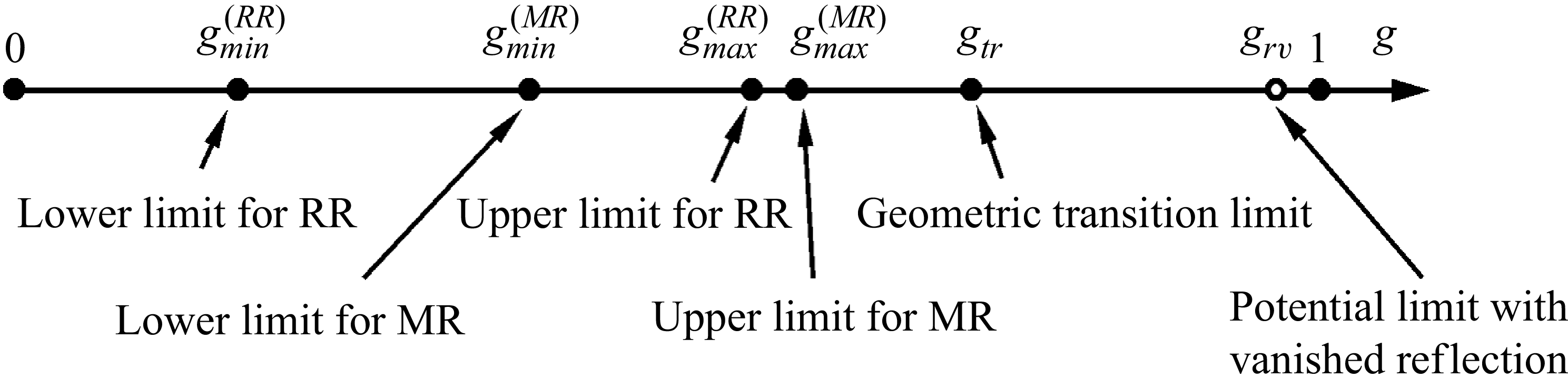
We have given in figures 5, 6, 8 and 9 the contour lines for the critical values
 $ g_{\textit{min}}^{(\textit{RR})}$
,
 $g_{\textit{min}}^{(\textit{MR})}$
,
 $g_{\textit{max}}^{(\textit{RR})}$
and
 $g_{\textit{max}}^{(\textit{MR})}$
, respectively. The relative positions of these critical values of
 $ g$
are displayed on the
 $g$
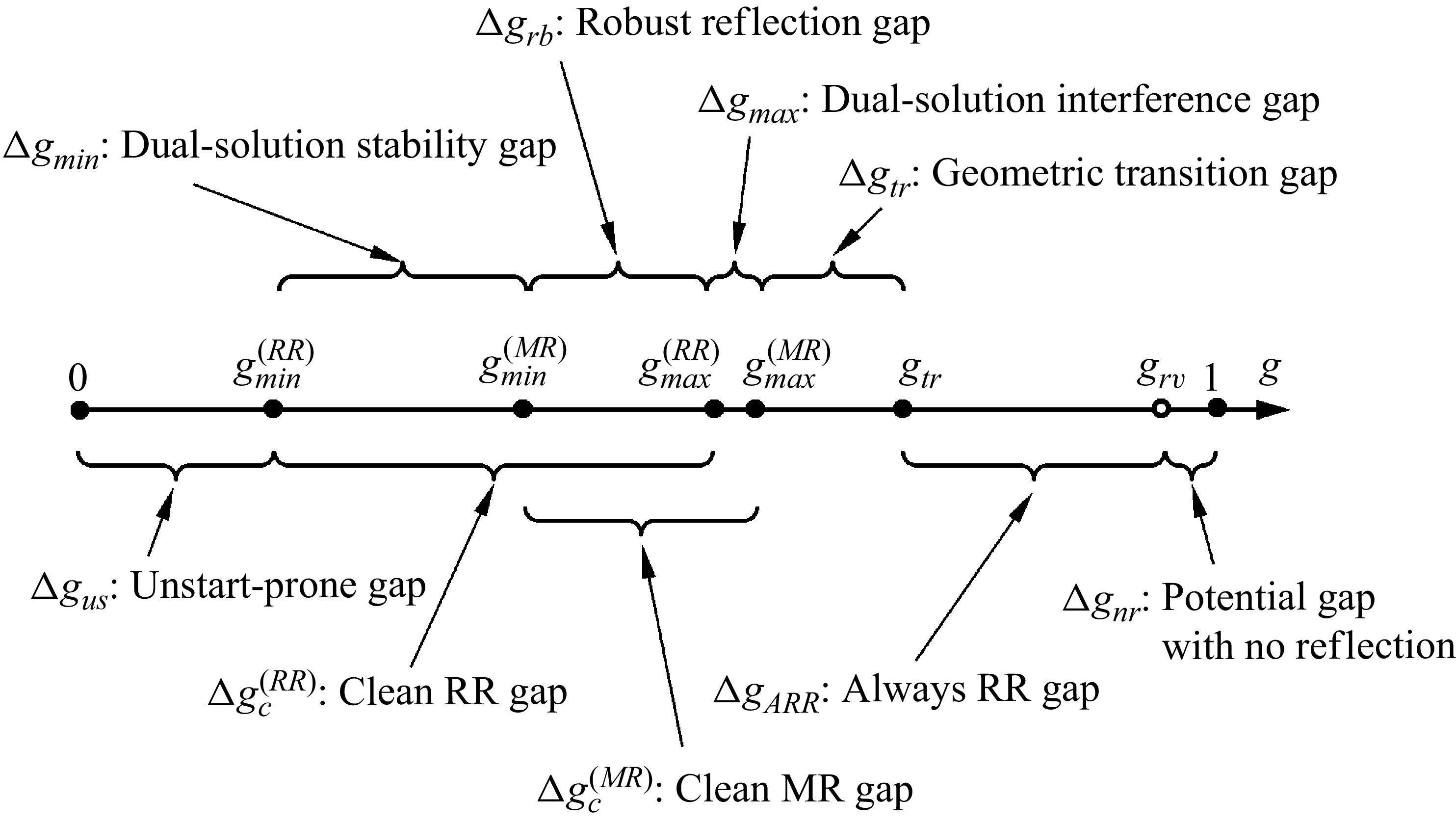
-axis in figure 12.
Six limits of
 $g$
along the
 $g$
-axis, plus a potential limit for no reflection.

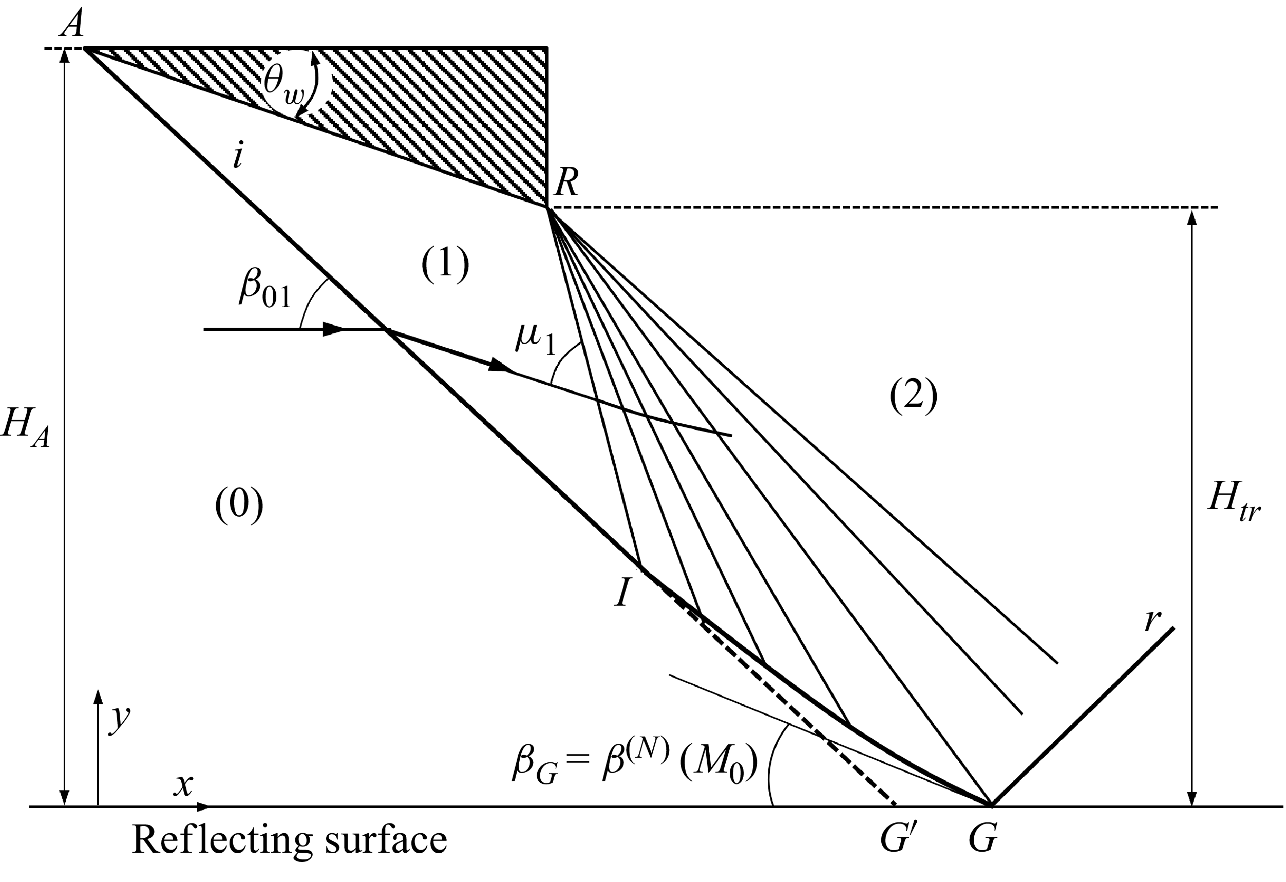
Figure 12 also marks the geometric transition criterion
 $g_{\textit{tr}}$
, at which the shock angle (
 $\beta _{G}$
) of the incident shock at the reflecting surface reaches its local von Neumann condition, due to weakening of the incident shock by the trailing edge expansion fan. At
 $g=g_{\textit{tr}}$
, the shock angle is the one at the von Neumann condition, i.e.
 \begin{align} \beta _{G}=\beta ^{(N)}(M_{0}), \end{align}
and the flow deflection angle at this point is determined by
 $\theta _{G}=\theta ^{(N)}(M_{0})$
, where
 $\tan \theta ^{(N)}=f_{\theta }(M_{0},\beta _{G})$
. The shock reflection has the configuration as displayed in figure 13. Above
 $g=g_{\textit{tr}}$
, MR will necessarily transit to RR. Since this transition is caused by a geometric set-up, it is called the geometric transition limit. Using methods of characteristics, Bai (Reference Bai2023, figure 6a) and Baby, Paramanantham & Rajesh (Reference Baby, Paramanantham and Rajesh2024, figure10b) obtained the values of
 $g_{\textit{tr}}$
in the
 $M_{0}{-}\theta _{w}$
plane.
In figure 12, we also marked a potential limit
 $g_{rv}$
above which there is no reflection. The possibility of the existence of such a critical value seems to have not been studied before, and will be considered shortly in § 5.4.
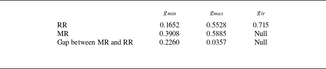
The relative positions of the various critical values displayed in figure 12 have not been given arbitrarily. They are based on the predicted values at the maximum point for the dual-solution domain, i.e. at
 $ M_{0}=6.2$
and
 $\theta _{w}=28.8^\circ$
. Table 3 summarises the predicted values.
Critical values of
 $g$
at the maximal point
 $M_{0}=6.2$
and
 $ \theta _{w}=28.8^\circ$
.

Table 3. Long description
A table comparing critical values for different scenarios. The table has three rows and four columns. The columns are labeled g min, g max, and g tr. The rows are labeled RR, MR, and Gap between MR and RR. Row 1: RR, g min 0.1652, g max 0.5528, g tr 0.715. Row 2: MR, g min 0.3908, g max 0.5885, g tr Null. Row 3: Gap between MR and RR, g min 0.2260, g max 0.0357, g tr Null.
Schematic display of the incident shock when
 $g=g_{\textit{tr}}$
.

In the previous sections, we have only given schematic displays of shock reflections at various critical values of
 $g$
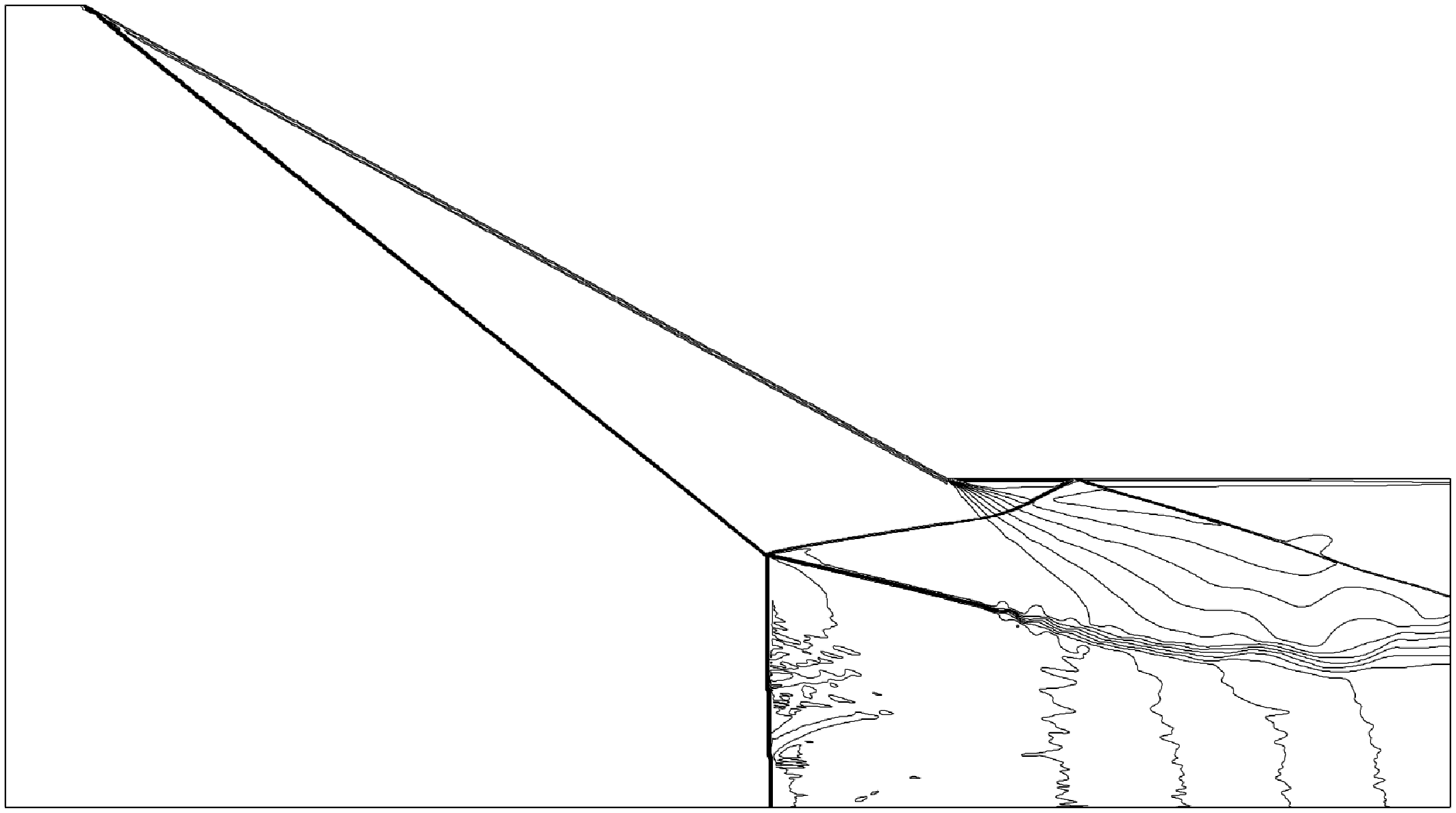
. In figure 14, we give the Mach number contour lines obtained by numerical simulation (performed by solving the Euler equations in gas dynamics, using the same approach as used by Wang & Wu 2026), for the conditions displayed in table 3 to show the shock reflection patterns.
Mach number contour lines at the maximum point
 $M_{0}=6.2$
and
 $ \theta _{w}=28.8^\circ$
, for (a)
 $g=g_{\textit{min}}^{(\textit{RR})}$
, (b)
 $g=g_{\textit{min}}^{(\textit{MR})}$
, (c)
 $g=g_{\textit{max}}^{(\textit{RR})}$
, (d)
 $g=g_{\textit{max}}^{(\textit{MR})}$
, (e)
 $g=g_{\textit{tr}}$
,.

Figure 14. Long description
Panel A: A diagram showing a simple triangular shape with straight lines. Panel B: A diagram with a triangular shape and multiple contour lines radiating from the right angle. Panel C: A diagram with a triangular shape and contour lines forming complex patterns near the right angle. Panel D: A diagram with a triangular shape and contour lines spreading out from the right angle. Panel E: A diagram with a triangular shape and contour lines radiating from the right angle, labeled with an angle of approximately 29 degrees.
At
 $g=g_{\textit{min}}^{(\textit{RR})}$
, the reflected shock indeed grasps the trailing edge, as can be seen from figure 14(a). At
 $g=g_{\textit{min}}^{(\textit{MR})}$
, the reflected shock has moved upstream of the trailing edge, as shown in figure 14(b) (a snapshot of the unsteady solution). At
 $g=g_{\textit{max}}^{(\textit{RR})}$
, the leading characteristics of the trailing edge expansion fan indeed intersects the incident shock at the reflecting surface, as is clear from figure 14(c). At
 $g=g_{\textit{max}}^{(\textit{MR})}$
, the leading characteristics of the trailing edge expansion fan indeed intersect the triple point, as is clear from figure 14(d). At
 $g=g_{\textit{tr}}$
, the incident shock reflects at a shock angle that is near the von Neumann condition (
 $\beta ^{(N)}(6.2)\approx 29^\circ$
), as shown in figure 14(e). To complement the result shown in figure 14(b), we have performed a further computation for
 $g=0.41$
, with which we have been able to obtain stable MR, as shown in figure 15. The fact that we have the unstable solution shown in figure 14(b) for
 $g=0.3908$
and the stable solution shown in figure 15 for
 $g=0.41$
means that the precise value of
 $g_{\textit{min}}^{(\textit{MR})}$
should satisfy
 $0.3908\lt g_{\textit{min}}^{(\textit{MR})}\lt 0.41$
. Thus the predicted
 $g_{\textit{min}}^{(\textit{MR})}$
is different from the real value by an error as small as
 $\approx 5\,\%$
.
Mach number contour lines at the maximum point
 $M_{0}=6.2$
and
 $ \theta _{w}=28.8^\circ$
, for
 $g=0.41$
.

5.2. Various gaps along the
$g$
-axis

The distance between adjacent geometric limits defines meaningful gaps, as displayed in figure 16, which shows eight gaps, plus a potential gap with no reflection (see § 5.4), as follows.
A full geometric picture defining six limits of
 $g$
and eight gaps along the
 $g$
-axis, plus a potential gap for vanished reflection.

-
(i) The unstart-prone reflection gap
$\Delta g_{us}$
, corresponding to
$ 0\lt g\lt g_{\textit{min}}^{(\textit{RR})}$
. In this gap, the reflected shock will touch the lower wedge surface, leading to unstart flow for MR (Vuillon et al. Reference Vuillon, Zeitoun and Ben-Dor1995), or shock reflection on the lower wedge surface for RR. For the latter case, the boundary layer in real flow will be subjected to shock wave/boundary layer interaction leading to possibly unsteady flow separation. -
(ii) The dual-solution stability gap
$\Delta g_{\textit{min}}$
: this is the gap between
$g_{\textit{min}}^{(\textit{RR})}$
and
$g_{\textit{min}}^{(\textit{MR})}$
, for which stable RR may transit to unstable MR under suitable disturbance (Wang & Wu 2026). -
(iii) The dual-solution interference gap
$\Delta g_{\textit{max}}$
: this is the gap between
$g_{\textit{max}}^{(\textit{RR})}$
and
$g_{\textit{max}}^{(\textit{MR})}$
. Within this gap, the incident shock interacts with the trailing edge expansion fan for RR, and not for MR. -
(iv) The geometric transition gap
$\Delta g_{\textit{tr}}$
: this is the gap between
$ g_{\textit{max}}^{(\textit{MR})}$
and
$g_{\textit{tr}}$
. When
$g\gt g_{\textit{max}}^{(\textit{MR})}$
, the weakening of the incident shock forces an MR to transit to RR when
$g\rightarrow g_{\textit{tr}}$
. -
(v) The clean RR gap
$\Delta g_{c}^{(\textit{RR})}$
: this is the gap between
$g_{\textit{min}}^{(\textit{RR})}$
and
$g_{\textit{max}}^{(\textit{RR})}$
. Within this gap, RR has no interaction between the incident shock and the trailing edge expansion fan, and the reflected shock will not grasp the trailing edge. More details are given in § 5.3. -
(vi) The clean MR gap
$\Delta g_{c}^{(\textit{MR})}$
: this is the gap between
$g_{\textit{min}}^{(\textit{MR})}$
and
$g_{\textit{max}}^{(\textit{MR})}$
. Within this gap, MR has no interaction between the incident shock and the trailing edge expansion fan, and the reflected shock will not grasp the trailing edge, i.e. MR can be stable. More details are given in § 5.3. -
(vii) The robust reflection gap
$\Delta g_{rb}$
: this is the gap between
$ g_{\textit{min}}^{(\textit{MR})}$
and
$g_{\textit{max}}^{(\textit{RR})}$
. The meaning of robust reflection will be described in § 5.3. -
(viii) The always RR gap
$\Delta g_{\textit{ARR}}$
: this is the gap between
$g_{\textit{tr}}$
and
$ g_{rv}$
, where we only have RR. -
(ix) Potential gap with no reflection
$\Delta g_{\textit{nr}}$
: this is the gap between the hypothetical
$g_{rv}$
and
$g=1$
.


The existence of
 $g_{rv}$
will be discussed shortly in § 5.4.
5.3. Clean and robust reflection gaps
Clean shock reflection (CSR) is defined here as the reflection for which the incident shock is not perturbed by the trailing edge expansion fan, and the reflected shock does not grasp the trailing edge. In terms of the range of
 $ g$
, the CSR gap is defined as
 $g_{\textit{min}}\lt g\lt g_{\textit{max}}$
. In terms of the distance between
 $g_{\textit{min}}$
and
 $g_{\textit{max}}$
, this CSR gap is defined by
 \begin{align} \Delta g_{c}=g_{\textit{max}}-g_{\textit{min}}. \end{align}
Figure 17 displays, for RR, the CSR gap
 $\Delta g_{c}$
in the
 $ M_{0}{-}\theta _{w}$
plane. It is seen that when
 $\theta _{w}\rightarrow 0$
, the CSR gap satisfies
 $\Delta g_{c}\rightarrow 0$
, meaning that for very weak shock waves the range of
 $g$
with CSR is narrow. At fixed
 $ M_{0}$
,
 $\Delta g_{c}$
has a maximal value at some
 $\theta _{w}=\theta _{w,m}$
, which is always below the von Neumann condition.
Contour lines (solid) of
 $\Delta g_{c}^{(\textit{RR})}=g_{\textit{max}}^{(\textit{RR})}-g_{\textit{min}}^{(\textit{RR})}$
in the
 $M_{0}{-}\theta _{w}$
plane. Dashed lines represent critical conditions.

Figure 18 displays, for MR, the CSR gap
 $\Delta g_{c}$
in the
 $ M_{0}{-}\theta _{w}$
plane. It is seen that when
 $\theta _{w}\rightarrow \theta _{\textit{max}}$
, the CSR gap satisfies
 $\Delta g_{c}\rightarrow 0$
, meaning that for very strong shock waves, the range of
 $g$
with CSR is narrow. At fixed
 $M_{0}$
,
 $\Delta g_{c}$
increases monotonically for
 $ \theta _{w}$
varying from
 $\theta _{\textit{max}}$
to
 $\theta _{w}^{(N)}$
. Thus the maximum values of
 $\Delta g_{c}$
occur near
 $\theta _{w}\rightarrow \theta _{w}^{(N)}$
for MR, unlike RR for which the maximum value of
 $ \Delta g_{c}$
occurs at
 $\theta _{w}\rightarrow \theta _{w}^{(D)}$
.
Contour lines (solid) of
 $\Delta g_{c}^{(\textit{MR})}=g_{\textit{max}}^{(\textit{MR})}-g_{\textit{min}}^{(\textit{MR})}$
in the
 $M_{0}{-}\theta _{w}$
plane. Dashed lines represent critical conditions.

Figure 18. Long description
A line graph with contour lines (solid) and critical conditions (dashed lines) in the plane. The horizontal axis is labeled M 0 ranging from 2.5 to 7.0. The vertical axis is labeled theta w (degrees) ranging from 15 to 40. The graph includes multiple solid contour lines labeled with values such as 0.01, 0.06, 0.11, 0.16, 0.21, 0.26, 0.31, 0.36, 0.41, and 0.46. The dashed lines represent critical conditions labeled as theta max, theta w superscript D, and theta w superscript N. An arrow indicates an increase in a specific direction.
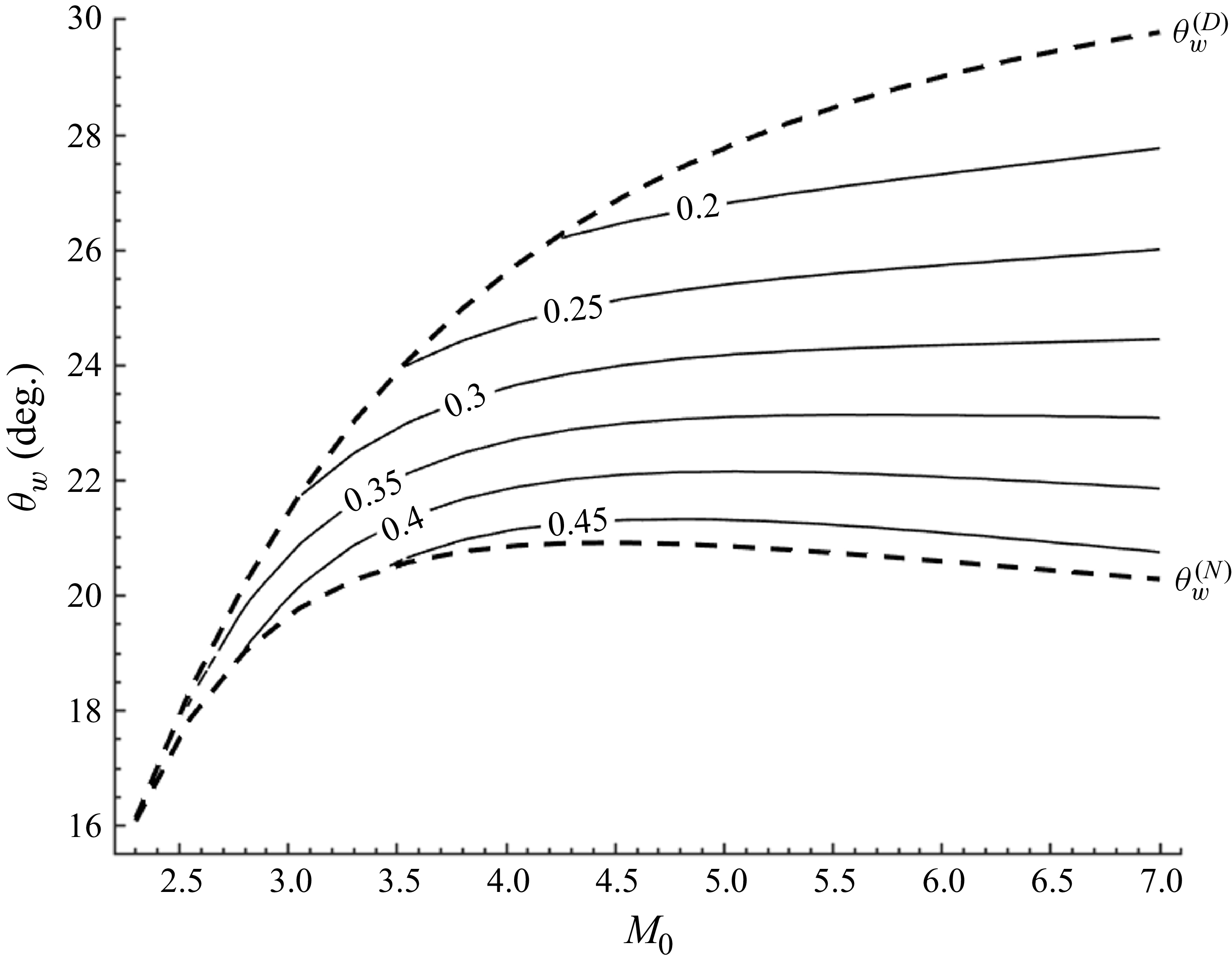
The robust reflection gap
 $\Delta g_{rb}=g_{\textit{max}}^{(\textit{RR})}-g_{\textit{min}}^{(\textit{MR})}$
, as shown in figure 16, defines the range of
 $g$
with which the incident shock is free of interaction with the trailing edge expansion fan, and the reflected shock has no risk of grasping the trailing edge, whenever the reflection is RR and MR, or may undergo transition between RR and MR. This gap, computed by using the values of
 $g_{\textit{min}}^{(\textit{MR})}$
displayed in figure 6 and
 $g_{\textit{max}}^{(\textit{RR})}$
displayed in figure 8, is displayed in figure 19.
The robust reflection gap
 $\Delta g_{c}=g_{\textit{max}}^{(\textit{RR})}-g_{\textit{min}}^{(\textit{MR})}$
in the dual-solution domain.

Comparing figures 7, 10 and 19, we see that the robust reflection gap is the largest, while the dual-solution interference gap is the smallest.
5.4. The potential existence of
$g_{rv}$
and
$\Delta g_{\textit{nr}}$


Now consider the possibility
 $g=g_{rv}$
, beyond which there is no reflection. This means that at
 $g=g_{rv}$
, we would have
 $\beta _{G}=\mu (M_{0})$
, i.e. at the reflecting point, the incident shock degenerates to a Mach wave.
Figure 20(a) is a schematic display of the hypothetical configuration at
 $g=g_{rv}$
. The incident shock just degenerates to a Mach wave at the reflecting surface, and the reflected wave is also a Mach wave. Figure 20(b) is a schematic display of the hypothetical configuration of no reflection for
 $g\gt g_{rv}$
. There is a hypothetical death point (
 $D$
) that marks the end of the incident shock, below which the incident shock degenerates to a Mach wave. One would ask if the existence of
 $g_{rv}$
with
 $g_{rv}\lt 1$
can be theoretically justified.
Schematic display of vanishing reflection, for (a)
 $g=g_{rv}$
, (b)
 $ g\gt g_{rv}$
.

Figure 20. Long description
Panel A: A schematic diagram showing the vanishing reflection phenomenon. The diagram includes a reflecting surface labeled as G, and various regions labeled as 0, 1, and 2. The diagram shows the interaction of a Mach wave with the reflecting surface. Key points include A, R, and G, with angles labeled as beta 01, i, and mu 1. The vertical axis is labeled H A and the horizontal axis is labeled H rv. Panel B: A schematic diagram showing another configuration of the vanishing reflection phenomenon. This diagram also includes a reflecting surface labeled as G, and regions labeled as 0, 1, and 2. The diagram shows the interaction of a shock wave and a degenerated Mach wave with the reflecting surface. Key points include A, R, and D, with angles labeled as beta 01, i, and mu 1. The vertical axis is labeled H A and the horizontal axis is labeled H rv.
When
 $g\rightarrow 1$
, the initial point of the incident shock approaches the trailing edge expansion fan infinitely, so it will degenerate into a Mach wave, meaning that there is no shock reflection.
To see whether
 $g_{rv}\lt 1$
, we display some numerical results with
 $g$
approaching
 $1$
. We give in figure 21 the Mach number contour lines for
 $g=0.82$
,
 $0.95$
,
 $0.99$
and
 $0.995$
, at
 $M_{0}=6.2$
and
 $\theta _{w}=28.8^\circ$
.
Compared to figure 14(e), with
 $g=g_{\textit{tr}}=0.71$
and
 $\beta _{G}\approx 29^\circ$
(close to the von Neumann condition
 $\beta ^{(N)}(M_{0})=28.6^\circ$
), here with
 $g=0.82$
, the incident shock has shock angle
 $\beta _{G}\approx 22.3^\circ$
, which is well below the von Neumann condition. For
 $g=0.95$
, the incident shock has shock angle
 $\beta _{G}\approx 12.7^\circ$
at the reflecting surface; see figure 21(b). For
 $g=0.99$
, the incident shock appears to be as weak as a Mach wave, but at the reflecting point, the incident shock has shock angle
 $\beta _{G}\approx 11.1^\circ$
, which is still well above the Mach angle
 $\mu =\arcsin ( {1}/{ M_{0}})= 9.28^\circ$
; see figure 21(c). Figure 21(d) corresponds to
 $g=0.995$
and shows that
 $\beta _{G}\approx 10.4^\circ$
, which is close to but still slightly larger than the Mach angle
 $\mu = 9.28^\circ$
.
Mach number contourlines at the maximum point
 $M_{0}=6.2$
and
 $ \theta _{w}=28.8$
 $^{\circ}$
(a)
 $g=0.82$
, (b)
 $g=0.95$
, (c)
 $g=0.99$
, (d)
 $ g=0.995$
.

Despite it being anticipated that no reflection occurs when
 $g\rightarrow 1$
, we have not yet observed the appearance of such a limit
 $g_{\textit{nr}}$
, with
 $ g_{\textit{nr}}\lt 1$
, through numerical simulation with
 $g$
as large as
 $0.995$
.
For a sonic boom, a supersonic vehicle generates shock waves and expansion waves, which interact so that there is a sonic boom even at large distance (Reference CrowCrow1969; Carlson Reference Carlson1978). There appears to be no cut-off point at which the shock degenerates into a Mach wave, but the strength of the shock wave will decay gradually.
For the present problem, one would expect to prove analytically whether there is a reflection vanishing
 $g_{rv}$
satisfying
 $g_{rv}\lt 1$
. The problem of interaction between an expansion fan and a shock wave has been studied before (Moeckel Reference Moeckel1952; Rosciszewski Reference Rosciszewski1960; Hasimoto Reference Hasimoto1964; Li & Ben-Dor Reference Li and Ben-Dor1995; Meshkov et al. Reference Meshkov, Omelchenko and Uskov2002; Hillier Reference Hillier2007; Silnikov et al. Reference Silnikov, Chernyshov and Uskov2014; Uskov & Chernyshov Reference Uskov and Chernyshov2014; Bai Reference Bai2023; Baby et al. Reference Baby, Paramanantham and Rajesh2024). When the expansion wave is upstream of the shock, analytical solutions can be found (Silnikov et al. Reference Silnikov, Chernyshov and Uskov2014; Uskov & Chernyshov Reference Uskov and Chernyshov2014). In the present problem, the shock and the expansion fan in interaction are in the same side, and the expansion fan is downstream of the shock wave, so there is no analytical solution. Methods by characteristics (Hillier Reference Hillier2007; Bai Reference Bai2023; Baby et al. Reference Baby, Paramanantham and Rajesh2024) are approximate in nature and do not allow us to make a rigorous mathematical claim that there exists a
 $ g_{rv}$
with
 $g_{rv}\lt 1$
. Thus the existence of
 $g_{rv}$
remains an open question. Hasimoto (Reference Hasimoto1964) derived the curvature of the shock at the starting point of interaction between this shock and a downstream expansion fan from the same side. It is unclear whether this analytical approach can be extended to study the properties of the entire part of the shock under interaction.
6. Conclusions
The lower and upper limits of the trailing edge height in the conventional wedge-induced steady shock reflection problem are important parameters, as they determine the stability or the configuration of the shock reflection. Both limits depend on the Mach stem height in the case of Mach reflection (MR). Previously, the lack of an accurate and sufficiently simple Mach stem height model made it impossible to estimate these limits with acceptable accuracy across the entire parameter space. Thanks to the calibrated model for the Mach stem height recently proposed by Li & Bai (Reference Li and Bai2026), this obstacle is overcome.
The main contribution of the present work is threefold. First, we have derived explicit algebraic expressions for the lower limits
 $ g_{\textit{min}}^{(\textit{RR})}$
and
 $g_{\textit{min}}^{(\textit{MR})}$
and the upper limits
 $g_{\textit{max}}^{(\textit{RR})}$
and
 $g_{\textit{max}}^{(\textit{MR})}$
. These expressions transform previously implicit or numerically expensive relations into ready-to-use analytical tools valid over a wide range of
 $M_{0}$
and
 $\theta _{w}$
. Second, using these explicit formulas, we have discovered previously unknown qualitative behaviours: a maximum point of the dual-solution stability gap
 $\Delta g_{\textit{min}}$
at
 $M_{0}\approx 6.2$
,
 $\theta _{w}\approx 28.8^\circ$
; a systematic classification of eight distinct gaps along the
 $g$
-axis, including the clean reflection gap, the robust reflection gap, and the always-RR gap; and the demonstration that the dual-solution interference gap
 $\Delta g_{\textit{max}}$
is very small (less than 0.05 for
 $2.3\lt M_{0}\lt 7$
), implying that once the trailing edge expansion fan interacts with the incident shock in RR, it almost immediately interacts in MR as well. Third, we have discussed a potential reflection-vanished limit
 $g_{rv}$
, which raises a new open question for future investigation.
Taken together, these results provide the first complete quantitative picture of steady shock reflection along the entire
 $g$
-axis, from
 $g=0$
to
 $ g=1$
. The explicit algebraic expressions and the identified gaps offer practical guidance for experimental design and numerical simulation, while the new physical insights deepen our understanding of how the third geometric parameter
 $g$
governs the transition, stability and interference patterns of shock reflection.
Acknowledgements
The authors would like to thank all the referees for their valuable comments leading to improvement of the paper.
Funding
This work was supported partly by the National Key Project (grant no. GJXM92579) and by the National Science and Technology Major Project 2017-II-003-0015.
Declaration of interests
The authors report no conflict of interest.

 HR
 HR,min
 HR,max
 HR=HR,min

 HR=HR,max

 gmin(RR)
 M0−θw

 gmin(MR)
 M0−θw
 gmin
 gmin
 gmin
 gmin

 Δgmin=gmin(MR)−gmin(RR)
 Δgmin

 gmax(RR)
 M0−θw

 gmax(MR)
 M0−θw
 Δgmax=gmax(MR)−gmax(RR)
 Δgmax=gmax(MR)−gmax(RR)
 g
 g
 g
 M0=6.2
 θw=28.8∘
 g=gtr

 M0=6.2
 θw=28.8∘
 g=gmin(RR)
 g=gmin(MR)
 g=gmax(RR)
 g=gmax(MR)
 g=gtr
 M0=6.2
 θw=28.8∘
 g=0.41
 g
 g

 Δgc(RR)=gmax(RR)−gmin(RR)
 M0−θw

 Δgc(MR)=gmax(MR)−gmin(MR)
 M0−θw
 Δgc=gmax(RR)−gmin(MR)

 g=grv
 g>grv

 M0=6.2
 θw=28.8
 ∘
 g=0.82
 g=0.95
 g=0.99
 g=0.995


