2 Steady-state distribution

In this section, the problem of finding a stationary distribution for trapped electrons is considered. A possible way of finding a steady-state distribution, if it exists, is by considering the transient in which electrons are emitted by the sphere. As the dynamics of free and trapped electrons are completely independent, as discussed in § 1, only the phase in which all the (new) emitted electrons are trapped is considered here. This can be done simply by imposing an initial positive charge on the spherical body, $Q_{S}(0)=Q_{0}>0$ . In practice, the charge $Q_{0}$ is due to the previous emission of (free) electrons or to other causes (e.g. the emission of a high-energy electron beam, as in space experiments). If $eQ_{0}/R$ is larger than $(1/2)mv_{0}^{2}$ , all the electrons are confined by the potential of the sphere. At time $t$ , an electric charge, $Q_{e}(t)<0$ , due to the electrons will be present outside the body, and, consequently, the charge of the body is $Q_{S}(t)=Q_{0}-Q_{e}=Q_{0}+|Q_{e}|$ . 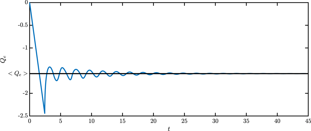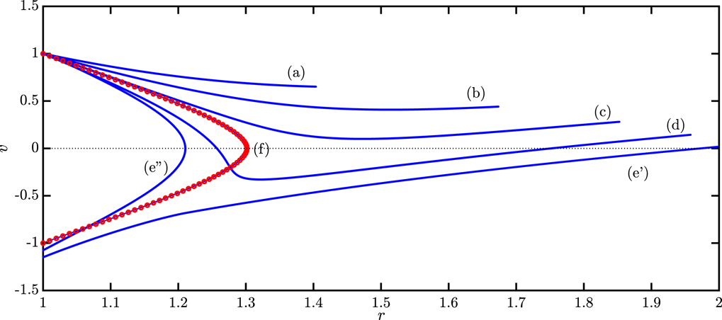Typical numerical results are presented in figures 1–4. The numerical simulation of the transients has been performed by using the ‘shell’ method (Boella et al. Reference Boella, Coppa, D’Angola and Peiretti Paradisi2018). The method uses computational particles in the shape of spherical shells, and the electric field is evaluated with Gauss’s theorem on a shell of radius $r$ by summing the charges of the particles included in the shell without using a computational grid. In this way, no boundary conditions are necessary for the electric potential. The shell method provides accurate, noiseless results that can be regarded as a reference.

Figure 1.

Damped oscillations for the total electron charge outside the sphere. Dimensionless units are used, as described in the text. The normalized electron flux, $I_{0}$ , and the normalized initial charge on the sphere, $Q_{0}$ , are both set equal to 1.

Figure 2.

Oscillating behaviour of the total electron charge. For this case, $I_{0}=2$ and $Q_{0}=1$ have been chosen.

For different values of the parameters, the evolution of $Q_{e}$ presents two different situations: damped oscillations (figure 1), or oscillating behaviour (figure 2). The corresponding phase-space distributions are shown in figures 3 and 4 (in these figures, as for all the results presented in the paper, lengths are normalized to $R$ , times to $R/v_{0}$ , charges to $mv_{0}^{2}R/e$ , particle fluxes to $mv_{0}^{3}/e^{2}$ ). These results suggest that a stationary solution for the phase-space distribution may exist, at least if the parameters of the problem, $Q_{S},v_{0},I_{0}$ , are in a given domain. The steady-state solution can be easily found by using the Poisson equation for the electric potential

(2.1) $$\begin{eqnarray}\displaystyle {\displaystyle \frac{1}{r^{2}}}{\displaystyle \frac{\text{d}}{\text{d}r}}\left(r^{2}{\displaystyle \frac{\text{d}\unicode[STIX]{x1D6F7}}{\text{d}r}}\right)=-4\unicode[STIX]{x03C0}\unicode[STIX]{x1D70C}, & & \displaystyle\end{eqnarray}$$

and considering that, for a stationary flow of electrons, one can write the charge density $\unicode[STIX]{x1D70C}$ as:

(2.2) $$\begin{eqnarray}\displaystyle \unicode[STIX]{x1D70C}=-{\displaystyle \frac{1}{4\unicode[STIX]{x03C0}r^{2}}}{\displaystyle \frac{2eI_{0}}{v(r)}} & & \displaystyle\end{eqnarray}$$

(the factor 2 is justified by noticing that, for a given $r$ , electrons move with velocity $+v(r)$ and $-v(r)$ ). The velocity $v(r)$ is calculated by considering that ${\mathcal{E}}=(1/2)mv_{0}^{2}-e\unicode[STIX]{x1D6F7}(r)$ is a constant of the motion (assuming $\unicode[STIX]{x1D6F7}(R)=0$ , ${\mathcal{E}}$ is simply equal to $(1/2)mv_{0}^{2}$ ). Finally, by introducing the potential energy for an electron, $U(r)=-e\unicode[STIX]{x1D6F7}(r)$ and using equations (2.1), (2.2), one eventually obtains the equation:

(2.3) $$\begin{eqnarray}\displaystyle {\displaystyle \frac{\text{d}}{\text{d}r}}\left(r^{2}{\displaystyle \frac{\text{d}U}{\text{d}r}}\right)=-{\displaystyle \frac{2e^{2}I_{0}}{\left[\displaystyle \frac{2}{m}({\mathcal{E}}-U)\right]^{1/2}}}, & & \displaystyle\end{eqnarray}$$

to be solved with the initial conditions:

(2.4a,b ) $$\begin{eqnarray}\displaystyle U(R)=0,\quad {\displaystyle \frac{\text{d}U}{\text{d}r}}(R)={\displaystyle \frac{eQ_{S}}{R^{2}}}, & & \displaystyle\end{eqnarray}$$

as $\text{d}U/\text{d}r=-e\text{d}\unicode[STIX]{x1D6F7}/\text{d}r=eE(r)$ and $E(R)=Q_{S}/R^{2}$ . Although (2.3) is well known (it was initially considered by Langmuir & Blodgett (Reference Langmuir and Blodgett1924) studying an electron diode), in the present case the interest is not in the electron flow between two electrodes, but in the motion of trapped particles, which return to the same electrode. Therefore the solution of (2.3) presents some peculiarities, as it must be solved in the $r-$ interval $[R,r_{max}]$ , with $r_{max}$ the turning point for the electrons, for which ${\mathcal{E}}-U(r_{max})=0$ . Equivalently, equation (2.3) can be cast into two first-order differential equations:

(2.5) $$\begin{eqnarray}\displaystyle \left.\begin{array}{@{}l@{}}\displaystyle {\displaystyle \frac{\text{d}U}{\text{d}r}}={\displaystyle \frac{\unicode[STIX]{x1D6F9}}{r^{2}}},\quad U(R)=0,\\ \displaystyle {\displaystyle \frac{\text{d}\unicode[STIX]{x1D6F9}}{\text{d}r}}=-{\displaystyle \frac{2e^{2}I_{0}}{\left[\displaystyle \frac{2}{m}({\mathcal{E}}-U)\right]^{1/2}}},\quad \unicode[STIX]{x1D6F9}(R)=eQ_{S}.\end{array}\right\} & & \displaystyle\end{eqnarray}$$

Equation (2.3), or system (2.5), must be solved numerically, but a direct solution presents two problems: (i) $r_{max}$ is unknown; (ii) $({\mathcal{E}}-U)^{-1/2}$ diverges when $r\rightarrow r_{max}$ . On the other hand, the range for $U$ is known, as $U\in [0,{\mathcal{E}}]$ , and therefore $U$ itself can be used as independent variable (i.e. $r=r(U)$ and $\unicode[STIX]{x1D6F9}=\unicode[STIX]{x1D6F9}(U)$ ), giving

(2.6) $$\begin{eqnarray}\displaystyle \left.\begin{array}{@{}l@{}}\displaystyle {\displaystyle \frac{\text{d}r}{\text{d}U}}={\displaystyle \frac{r^{2}}{\unicode[STIX]{x1D6F9}}},\quad r(U=0)=R,\\ \displaystyle {\displaystyle \frac{\text{d}\unicode[STIX]{x1D6F9}}{\text{d}U}}=-{\displaystyle \frac{r^{2}}{\unicode[STIX]{x1D6F9}}}{\displaystyle \frac{2e^{2}I_{0}}{\left[\displaystyle \frac{2}{m}({\mathcal{E}}-U)\right]^{1/2}}},\quad \unicode[STIX]{x1D6F9}(U=0)=eQ_{S}.\end{array}\right\} & & \displaystyle\end{eqnarray}$$

Figure 3.

Phase-space evolution for the electron distribution in the same case as figure 1. The different curves a,b,c,d,e’-e”, f, correspond to different times $t=0.5,1,1.5,2,2.5,100$ . The steady-state solution (from system (2.7)) is also presented (circles).

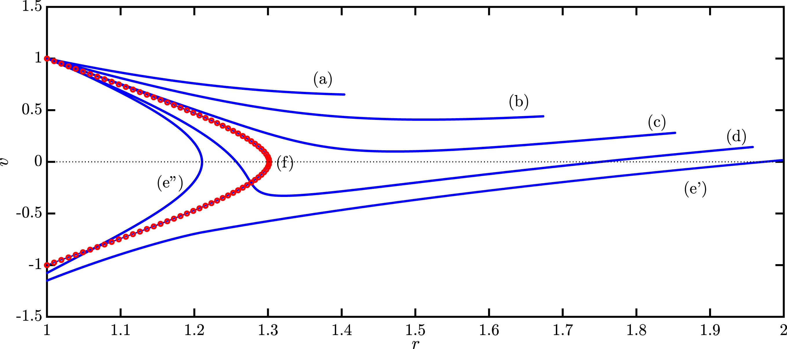
Finally, the singularity for $U\rightarrow {\mathcal{E}}$ can be eliminated by using the momentum $p=\{2m({\mathcal{E}}-U)\}^{1/2}$ as independent variable:

(2.7) $$\begin{eqnarray}\displaystyle \left.\begin{array}{@{}l@{}}\displaystyle {\displaystyle \frac{\text{d}r}{\text{d}p}}=-{\displaystyle \frac{p}{m}}{\displaystyle \frac{r^{2}}{\unicode[STIX]{x1D6F9}}},\quad r(p_{0})=R,\\ \displaystyle {\displaystyle \frac{\text{d}\unicode[STIX]{x1D6F9}}{\text{d}p}}=2e^{2}I_{0}{\displaystyle \frac{r^{2}}{\unicode[STIX]{x1D6F9}}},\quad \unicode[STIX]{x1D713}(p_{0})=eQ_{S},\end{array}\right\} & & \displaystyle\end{eqnarray}$$

with $p\in [0,p_{0}]$ and $p_{0}=mv_{0}$ . An example of the solution of this equation is shown in figure 3, where the phase-space distribution obtained by (2.7) is compared with the asymptotic distribution as obtained with the shell method. As the system presents damped oscillation, one must expect a complete agreement between these two distributions. This is confirmed by the results presented in the figure.

Figure 4.

Phase-space distribution for the electrons at different times covering the period of an oscillation, for the same case as figure 2.

System (2.7) can be rewritten by introducing the new dimensionless quantities $\bar{r}=r/R$ , $\bar{p}=p/p_{0}$ and $\overline{\unicode[STIX]{x1D6F9}}=\unicode[STIX]{x1D6F9}/(eQ_{S})$ , as

(2.8) $$\begin{eqnarray}\displaystyle \left.\begin{array}{@{}l@{}}\displaystyle {\displaystyle \frac{\text{d}\bar{r}}{\text{d}\bar{p}}}=-2\left({\displaystyle \frac{eQ_{S}/R}{{\mathcal{E}}}}\right)^{-1}\bar{p}{\displaystyle \frac{\bar{r}^{2}}{\overline{\unicode[STIX]{x1D6F9}}}},\quad \bar{r}(1)=1,\\ \displaystyle {\displaystyle \frac{\text{d}\overline{\unicode[STIX]{x1D6F9}}}{\text{d}\bar{p}}}=2\left({\displaystyle \frac{eQ_{S}/R}{{\mathcal{E}}}}\right)^{-2}\left({\displaystyle \frac{e^{2}N_{0}}{{\mathcal{E}}}}\right){\displaystyle \frac{\bar{r}^{2}}{\overline{\unicode[STIX]{x1D6F9}}}},\quad \overline{\unicode[STIX]{x1D6F9}}(1)=1,\end{array}\right\} & & \displaystyle\end{eqnarray}$$

with $\bar{p}\in [0,1]$ . Equations (2.8) show that the dynamics of the beam depends on two dimensionless parameters: $eQ_{S}/R/{\mathcal{E}}$ and $e^{2}N_{0}/{\mathcal{E}}$ .

Figure 5.

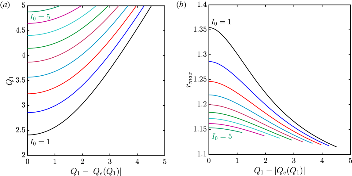
(a) Charge on the sphere, $Q_{1}$ , as a function of the total charge of the system, $Q_{1}+Q_{e}$ for $I_{0}$ in the range $1\div 5$ (with step 0.5). (b) Maximum value of the radial coordinate of the electron distribution, $r_{max}$ , as a function of $Q_{1}+Q_{e}$ for the same values of $I_{0}$ .

By solving system (2.7) all the physical quantities, in particular, the electron charge $Q_{e}=[\unicode[STIX]{x1D6F9}(r_{max})-\unicode[STIX]{x1D6F9}(R)]/e$ , can be calculated as a function of the charge on the sphere, $Q_{S}$ . In other words, having fixed all the other physical parameters, the function $Q_{e}(Q_{S})$ is obtained, representing the electron charge in equilibrium with the charge $Q_{S}$ on the sphere. In a real situation, one can imagine an initial condition with a charge $Q_{0}$ on the sphere and $Q_{e}=0$ . As the total charge is conserved, after the transient the charge on the sphere becomes $Q_{1}=Q_{0}+|Q_{e}(Q_{1})|$ . If $Q_{0}$ is known, the equation $Q_{1}-|Q_{e}(Q_{1})|=Q_{0}$ must be solved with respect to $Q_{1}$ . This can be done graphically, as shown in figure 5(a), where the curves of parametric equation $x=Q_{1}-|Q_{e}(Q_{1})|,y=Q_{1}$ are plotted for different values of $I_{0}$ . In the figure, each curve represents the value of the charge on the sphere after the transient, $Q_{1}$ , as a function of its initial value $Q_{0}$ . One can observe that the curves are defined if $Q_{0}>0$ . When $Q_{0}\rightarrow 0^{+}$ , the electric field for $r=r_{max}$ tends to 0, and the right-hand sides of the two equations (2.7) become singular. For this case, system (2.7) must be solved with ‘initial’ conditions

(2.9a,b ) $$\begin{eqnarray}\displaystyle U(r_{max})={\mathcal{E}},\quad \unicode[STIX]{x1D6F9}(r_{max})=0. & & \displaystyle\end{eqnarray}$$

A solution for this particular case is provided in the following. By making use of the kinetic energy $K={\mathcal{E}}-U$ instead of $U$ , and defining suitable dimensionless variables:

(2.10a-c ) $$\begin{eqnarray}\displaystyle s=1-r/r_{max},\quad \widetilde{K}=K/K_{1},\quad \widetilde{\unicode[STIX]{x1D6F9}}=\unicode[STIX]{x1D6F9}/\unicode[STIX]{x1D6F9}_{1}, & & \displaystyle\end{eqnarray}$$

with $K_{1}=[2e^{2}I_{0}/(2/m)^{1/2}]^{2/3}$ and $\unicode[STIX]{x1D6F9}_{1}=K_{1}r_{max}$ , system (2.7) becomes:

(2.11) $$\begin{eqnarray}\displaystyle \left.\begin{array}{@{}l@{}}\displaystyle {\displaystyle \frac{\text{d}\widetilde{K}}{\text{d}s}}={\displaystyle \frac{\widetilde{\unicode[STIX]{x1D6F9}}}{(1-s)^{2}}},\quad \widetilde{K}(s=0)=0,\\ \displaystyle {\displaystyle \frac{\text{d}\widetilde{\unicode[STIX]{x1D6F9}}}{\text{d}s}}={\displaystyle \frac{1}{\widetilde{K}^{1/2}}},\quad \widetilde{\unicode[STIX]{x1D6F9}}(s=0)=0.\end{array}\right\} & & \displaystyle\end{eqnarray}$$

If $s\ll 1$ , the denominator in the first (2.11) can be approximated by 1, and system (2.11) admits a simple analytic solution:

(2.12a,b ) $$\begin{eqnarray}\displaystyle \widetilde{K}(s)=({\textstyle \frac{9}{4}})^{2/3}s^{4/3},\quad \widetilde{\unicode[STIX]{x1D6F9}}(s)={\textstyle \frac{4}{3}}({\textstyle \frac{9}{4}})^{2/3}s^{1/3}, & & \displaystyle\end{eqnarray}$$

as can be verified by inspection. In general, when $s$ is not negligible, one can write $\widetilde{K}$ and $\widetilde{\unicode[STIX]{x1D6F9}}$ as:

(2.13a,b ) $$\begin{eqnarray}\displaystyle \widetilde{K}(s)=({\textstyle \frac{9}{4}})^{2/3}s^{4/3}{\mathcal{T}}(s),\quad \widetilde{\unicode[STIX]{x1D6F9}}(s)={\textstyle \frac{4}{3}}({\textstyle \frac{9}{4}})^{2/3}s^{1/3}{\mathcal{W}}(s), & & \displaystyle\end{eqnarray}$$

and system (2.11) becomes

(2.14) $$\begin{eqnarray}\displaystyle \left.\begin{array}{@{}l@{}}\displaystyle {\displaystyle \frac{\text{d}{\mathcal{T}}}{\text{d}z}}={\displaystyle \frac{4}{3}}\left\{{\displaystyle \frac{{\mathcal{W}}}{(1-\text{e}^{z})^{2}}}-{\mathcal{T}}\right\},\quad {\mathcal{T}}(-\infty )=1,\\ \displaystyle {\displaystyle \frac{\text{d}{\mathcal{W}}}{\text{d}z}}={\displaystyle \frac{1}{3}}\left\{{\displaystyle \frac{1}{{\mathcal{T}}^{1/2}}}-{\mathcal{W}}\right\},\quad {\mathcal{W}}(-\infty )=1,\end{array}\right\} & & \displaystyle\end{eqnarray}$$

having introduced the new variable $z=\log (s)$ in order to eliminate the singularity for $s\rightarrow 0$ . Now the new system can be readily solved numerically. In addition, for $z\rightarrow -\infty$ , when $s\ll 1$ and ${\mathcal{T}},{\mathcal{W}}\simeq 1$ , one can write ${\mathcal{T}}=1+\unicode[STIX]{x1D70F}$ , ${\mathcal{W}}=1+w$ , with $|\unicode[STIX]{x1D70F}|,|w|\ll 1$ and $(1-\text{e}^{z})^{-2}\simeq 1+2\text{e}^{z}$ . By linearizing the equations, one obtains:

(2.15a,b ) $$\begin{eqnarray}\displaystyle {\mathcal{T}}(z)\sim 1+{\textstyle \frac{16}{15}}\text{e}^{z},\quad {\mathcal{W}}(z)\sim 1-{\textstyle \frac{2}{15}}\text{e}^{z}. & & \displaystyle\end{eqnarray}$$

It is worthwhile noticing that $\widetilde{K}(s)$ and $\widetilde{\unicode[STIX]{x1D6F9}}(s)$ are ‘universal’ functions, as they do not depend on the parameters of the specific problem. In particular, these functions can be used to calculate the value of $Q_{1}$ corresponding to $Q_{0}=0$ (as in figure 5 a) for different values of $I_{0}$ , by solving the equations:

(2.16) $$\begin{eqnarray}\displaystyle & \displaystyle {\displaystyle \frac{mv_{0}^{2}}{2}}=K_{1}\widetilde{K}(1-R/r_{max}), & \displaystyle\end{eqnarray}$$

(2.17) $$\begin{eqnarray}\displaystyle & \displaystyle eQ_{1}=K_{1}r_{max}\widetilde{\unicode[STIX]{x1D6F9}}(1-R/r_{max}). & \displaystyle\end{eqnarray}$$

After obtaining $r_{max}$ from (2.16), one has $Q_{1}(Q_{0}=0)$ from (2.17). It has been verified that the values of $Q_{1}(Q_{0}=0)$ obtained in this way are in perfect agreement with the results shown in figure 5(a).

3 Transient analysis

The rise of the instability of the steady states, as studied in § 2, can be explained qualitatively in a simple way. Starting from a steady-state configuration with charge $Q_{S}$ on the sphere and charge $Q_{e}(Q_{S})$ due to the electrons (thus with total charge $Q_{S}+Q_{e}(Q_{S})$ ), one can imagine adding a charge $\unicode[STIX]{x1D6FF}Q_{S}$ on the sphere. Now the equilibrium electron charge is $Q_{e}(Q_{S}+\unicode[STIX]{x1D6FF}Q_{S})\simeq Q_{e}(Q_{S})+\text{d}Q_{e}/\text{d}Q_{S}(Q_{S})\cdot \unicode[STIX]{x1D6FF}Q_{S}$ . As the total charge is now $Q_{S}+Q_{e}(Q_{S})+\unicode[STIX]{x1D6FF}Q_{S}$ , after a time $\unicode[STIX]{x1D70F}$ (approximately of the order of the transit time of the electrons from emission to reabsorption), the charge on the sphere must become $Q_{S}+\unicode[STIX]{x1D6FF}Q_{S}^{\prime }$ , such that

(3.1) $$\begin{eqnarray}\displaystyle Q_{S}+Q_{e}(Q_{S})+\unicode[STIX]{x1D6FF}Q_{S}=Q_{S}+\unicode[STIX]{x1D6FF}Q_{S}^{\prime }+Q_{e}(Q_{S}+\unicode[STIX]{x1D6FF}Q_{S}). & & \displaystyle\end{eqnarray}$$

In other words, after a time interval $\unicode[STIX]{x1D70F}$ , the charge excess on the sphere is

(3.2) $$\begin{eqnarray}\displaystyle \unicode[STIX]{x1D6FF}Q_{S}^{\prime }=\left[1-{\displaystyle \frac{\text{d}Q_{e}}{\text{d}Q_{S}}}(Q_{S})\right]\unicode[STIX]{x1D6FF}Q_{S}. & & \displaystyle\end{eqnarray}$$

After a time $n\cdot \unicode[STIX]{x1D70F}$ , the initial perturbation is multiplied by a factor $(1-\text{d}Q_{e}/\text{d}Q_{S})^{n}$ . Considering that $\text{d}Q_{e}/\text{d}Q_{S}$ is always non-negative, the perturbation causes damped oscillations if $\text{d}Q_{e}/\text{d}Q_{S}<2$ , otherwise their amplitude is amplified. Of course, this condition is only approximate, and the real threshold to the instability requires a rigorous analysis of the dynamics of the system, which is the subject of the present section. The technique employed here represents an extension of the Lagrangian method introduced by Akimov et al. (Reference Akimov, Schamel, Kolinsky, Ender and Kuznetsov2001, Reference Akimov, Schamel, Ender and Kuznetsov2003) for the study of the stability of a planar electron diode. However, the spherical geometry makes the problem intrinsically more complicated and, as will be shown in the following, only a mixed analytical–numerical solution is possible.

Figure 6.

Behaviour of ${\mathcal{R}}(t,t_{1})$ , for fixed $t$ , as a function of $t_{1}$ . Obviously, ${\mathcal{R}}(t,t_{1}=t)=R$ and there are no electrons at time $t$ if the emission time, $t_{1}$ , is larger than $t$ . As $t_{1}$ decreases, ${\mathcal{R}}(t,t_{1})$ increases until the time $t_{1}=t_{max}(t)$ for which ${\mathcal{R}}$ is maximum (in other words, ${\mathcal{R}}(t,t_{max}(t))$ is the maximum radial distance at time $t$ for any electron of the system). For $t_{1}<t_{max}(t)$ , ${\mathcal{R}}(t,t_{1})$ decreases, as electrons are moving back after reaching their maximum distance. Finally, all electrons emitted for $t_{1}<\tilde{t}(t)$ have been reabsorbed by the sphere.

First of all, the function ${\mathcal{R}}(t,t_{0})$ , which represents the radial position at time $t$ of an electron emitted by the sphere at time $t_{0}$ , is introduced, together with its velocity:

(3.3) $$\begin{eqnarray}\displaystyle {\mathcal{V}}(t,t_{0})={\displaystyle \frac{\unicode[STIX]{x2202}{\mathcal{R}}}{\unicode[STIX]{x2202}t}}(t,t_{0}). & & \displaystyle\end{eqnarray}$$

The time evolution of ${\mathcal{V}}$ is governed by the equation:

(3.4) $$\begin{eqnarray}\displaystyle {\displaystyle \frac{\unicode[STIX]{x2202}{\mathcal{V}}}{\unicode[STIX]{x2202}t}}(t,t_{0})=-{\displaystyle \frac{e}{m}}E({\mathcal{R}}(t,t_{0}),t), & & \displaystyle\end{eqnarray}$$

with $E(r,t)$ the electric field. As in the time interval $\text{d}t_{1}$ a number of electrons $I_{0}\text{d}t_{1}$ are emitted and they will have position ${\mathcal{R}}(t,t_{1})$ and velocity ${\mathcal{V}}(t,t_{1})$ at time $t$ , a phase-space distribution $f(r,v,t)$ can be defined as

(3.5) $$\begin{eqnarray}\displaystyle f(r,v,t)=\int I_{0}\,\text{d}t_{1}\unicode[STIX]{x1D6FF}(r-{\mathcal{R}}(t,t_{1}))\unicode[STIX]{x1D6FF}(v-{\mathcal{V}}(t,t_{1})). & & \displaystyle\end{eqnarray}$$

The quantity $f(r,v,t)\text{d}r\text{d}v$ represents the number of electrons in $[r,r+\text{d}r]$ with radial velocity within $[v,v+\text{d}v]$ . From $f(r,v,t)$ , the electron charge in the region $[r_{1},r_{2}]$ at time $t$ can be written as

(3.6) $$\begin{eqnarray}\displaystyle Q_{e}(r_{1},r_{2},t)=-e\int _{r_{1}}^{r_{2}}\text{d}r\int I_{0}\,\text{d}t_{1}\unicode[STIX]{x1D6FF}(r-{\mathcal{R}}(t,t_{1})). & & \displaystyle\end{eqnarray}$$

As the charged contained in a sphere of radius $r>R$ is given by

(3.7) $$\begin{eqnarray}\displaystyle Q(r,t)=Q_{S}(t)+Q_{e}(R,r,t), & & \displaystyle\end{eqnarray}$$

where $Q_{S}(t)$ is the charge of the sphere at time $t$ , the electric field $E({\mathcal{R}}(t,t_{0}),t)$ can be written as:

(3.8) $$\begin{eqnarray}\displaystyle E({\mathcal{R}}(t,t_{0}),t)={\displaystyle \frac{Q({\mathcal{R}}(t,t_{0}),t)}{{\mathcal{R}}^{2}(t,t_{0})}}. & & \displaystyle\end{eqnarray}$$

Making use of (3.6), the contribution of electrons to $Q({\mathcal{R}}(t,t_{0}),t)$ can be expressed as:

(3.9) $$\begin{eqnarray}\displaystyle Q_{e}(R,{\mathcal{R}}(t,t_{0}),t)=-eI_{0}\int \text{d}t_{1}\int _{R}^{{\mathcal{R}}(t,t_{0})}\unicode[STIX]{x1D6FF}(r-{\mathcal{R}}(t,t_{1}))\,\text{d}r, & & \displaystyle\end{eqnarray}$$

in which the value of the $r-$ integral is 1 if ${\mathcal{R}}(t,t_{1})\in [R,{\mathcal{R}}(t,t_{0})]$ , otherwise it vanishes. The typical behaviour of ${\mathcal{R}}(t,t_{1})$ as a function of $t_{1}$ is shown in figure 6. Once $t_{0}\in (\tilde{t}(t),t)$ is fixed, a new time, $\tilde{t}_{0}(t,t_{0})\neq t_{0}$ can be determined such that ${\mathcal{R}}(t,\tilde{t}_{0}(t,t_{0}))={\mathcal{R}}(t,t_{0})$ (as in figure 6). It must be noticed that $\tilde{t}_{0}<t_{max}$ if $t_{0}>t_{max}$ and vice versa. With reference to figure 6, one can conclude that, for $t_{0}>t_{max}$ :

(3.10) $$\begin{eqnarray}\displaystyle \int _{R}^{{\mathcal{R}}(t,t_{0})}\unicode[STIX]{x1D6FF}(r-{\mathcal{R}}(t,t_{1}))\,\text{d}r=\left\{\begin{array}{@{}l@{}}1\quad \text{for }t_{1}\in [\tilde{t},\tilde{t}_{0}]\cup [t_{0},t],\\ 0\quad \text{otherwise},\end{array}\right. & & \displaystyle\end{eqnarray}$$

and, consequently, from (3.9) one has:

(3.11) $$\begin{eqnarray}\displaystyle Q_{e}(R,{\mathcal{R}}(t,t_{0}),t)=-eI_{0}[t-t_{0}+\tilde{t}_{0}(t,t_{0})-\tilde{t}(t)]. & & \displaystyle\end{eqnarray}$$

Instead, for $t_{0}<t_{max}$ , equation (3.11) must be modified, as:

(3.12) $$\begin{eqnarray}\displaystyle Q_{e}(R,{\mathcal{R}}(t,t_{0}),t)=-eI_{0}[t-\tilde{t}_{0}(t,t_{0})+t_{0}-\tilde{t}(t)]. & & \displaystyle\end{eqnarray}$$

Finally, $Q(r,t)$ must be evaluated. To do this, one can start by writing the charge $Q(t,t_{0})$ ‘seen’ at time $t$ by the electron emitted at $t_{0}$ as:

(3.13) $$\begin{eqnarray}\displaystyle Q(t,t_{0})=Q_{S}(t)+Q_{e}(R,{\mathcal{R}}(t,t_{0}),t). & & \displaystyle\end{eqnarray}$$

Moreover, the total charge of the system $Q_{tot}=Q_{S}(t)+Q_{e}(R,r_{max}(t),t)$ is constant, and therefore one has:

(3.14) $$\begin{eqnarray}\displaystyle Q(t,t_{0}) & = & \displaystyle Q_{tot}+Q_{e}(R,{\mathcal{R}}(t,t_{0}),t)-Q_{e}(R,r_{max}(t),t)\nonumber\\ \displaystyle & = & \displaystyle Q_{tot}+eI_{0}|t_{0}-\tilde{t}_{0}(t,t_{0})|,\end{eqnarray}$$

making use of (3.11), (3.12) and noticing that if ${\mathcal{R}}(t,t_{0})=r_{max}(t)$ then $\tilde{t}_{0}(t,t_{0})=t_{0}=t_{max}(t)$ (as in figure 6). In summary, equations (3.3), (3.4), (3.8), (3.14) determine the electron dynamics.

In a steady-state situation, all the previous quantities depend upon $\unicode[STIX]{x1D706}\equiv t-t_{0}$ only. In particular, ${\mathcal{R}}(t,t_{0})=\overline{{\mathcal{R}}}(\unicode[STIX]{x1D706})$ and ${\mathcal{V}}(t,t_{0})=\overline{{\mathcal{V}}}(\unicode[STIX]{x1D706})$ . Moreover, in this case the curve of figure 6 is symmetric with respect to $t_{max}(t)=t-\mathbb{T}/2$ , with $\mathbb{T}$ the total time of the trajectory for a single electron (from emission to absorption) and where $t_{0}-\tilde{t}_{0}$ is equal to $\mathbb{T}-2\unicode[STIX]{x1D706}$ , for $\unicode[STIX]{x1D706}\in (0,\mathbb{T}/2)$ . Therefore, the previous equations become:

(3.15) $$\begin{eqnarray}\displaystyle \left.\begin{array}{@{}l@{}}{\displaystyle \frac{\text{d}\overline{{\mathcal{R}}}}{\text{d}\unicode[STIX]{x1D706}}}=\overline{{\mathcal{V}}},\quad \overline{{\mathcal{R}}}(\unicode[STIX]{x1D706}=0)=R,\\ {\displaystyle \frac{\text{d}\overline{{\mathcal{V}}}}{\text{d}\unicode[STIX]{x1D706}}}=-{\displaystyle \frac{e}{m}}\left({\displaystyle \frac{Q_{0}-2eI_{0}\unicode[STIX]{x1D706}}{\overline{{\mathcal{R}}}^{2}}}\right),\quad \overline{{\mathcal{V}}}(\unicode[STIX]{x1D706}=0)=v_{0},\end{array}\right\} & & \displaystyle\end{eqnarray}$$

for $\unicode[STIX]{x1D706}\in [0,\mathbb{T}/2]$ , with $Q_{0}=Q_{tot}+eI_{0}\mathbb{T}$ . For $\unicode[STIX]{x1D706}\in [\mathbb{T}/2,\mathbb{T}]$ , one has simply

(3.16a,b ) $$\begin{eqnarray}\displaystyle \overline{{\mathcal{R}}}(\unicode[STIX]{x1D706})=\overline{{\mathcal{R}}}(\mathbb{T}-\unicode[STIX]{x1D706}),\quad \overline{{\mathcal{V}}}(\unicode[STIX]{x1D706})=-\overline{{\mathcal{V}}}(\mathbb{T}-\unicode[STIX]{x1D706}). & & \displaystyle\end{eqnarray}$$

It can be readily proved that system (3.15) is equivalent to the ones in the previous sectionFootnote ¹ . To study a transient, a suitable perturbation is added to the steady-state solution, in the form:

(3.17) $$\begin{eqnarray}\displaystyle \left.\begin{array}{@{}l@{}}{\mathcal{R}}(t,t_{0})=\overline{{\mathcal{R}}}(\unicode[STIX]{x1D706})+\unicode[STIX]{x1D716}\widehat{{\mathcal{R}}}(\unicode[STIX]{x1D706})\text{e}^{\text{i}\unicode[STIX]{x1D714}t},\\ {\mathcal{V}}(t,t_{0})=\overline{{\mathcal{V}}}(\unicode[STIX]{x1D706})+\unicode[STIX]{x1D716}\widehat{{\mathcal{V}}}(\unicode[STIX]{x1D706})\text{e}^{\text{i}\unicode[STIX]{x1D714}t},\\ E(t,t_{0})=\overline{E}(\unicode[STIX]{x1D706})+\unicode[STIX]{x1D716}\widehat{E}(\unicode[STIX]{x1D706})\text{e}^{\text{i}\unicode[STIX]{x1D714}t},\end{array}\right\} & & \displaystyle\end{eqnarray}$$

in which $\unicode[STIX]{x1D716}\ll 1$ and $\unicode[STIX]{x1D714}\in \mathbb{C}$ . Of course, only the real (or the imaginary) parts of ${\mathcal{R}}$ and ${\mathcal{V}}$ define the real perturbation. After introducing definitions (3.17) into (3.3), (3.4), one obtains:

(3.18) $$\begin{eqnarray}\displaystyle \left.\begin{array}{@{}l@{}}\displaystyle {\displaystyle \frac{\text{d}\widehat{{\mathcal{R}}}}{\text{d}\unicode[STIX]{x1D706}}}=\widehat{{\mathcal{V}}}-\text{i}\unicode[STIX]{x1D714}\widehat{{\mathcal{R}}},\\ \displaystyle {\displaystyle \frac{\text{d}\widehat{{\mathcal{V}}}}{\text{d}\unicode[STIX]{x1D706}}}=-{\displaystyle \frac{e}{m}}\widehat{E}(\unicode[STIX]{x1D706})-\text{i}\unicode[STIX]{x1D714}\widehat{{\mathcal{V}}}.\end{array}\right\} & & \displaystyle\end{eqnarray}$$

In the following, $E({\mathcal{R}}(t,t_{0}),t)$ and $Q({\mathcal{R}}(t,t_{0}),t)$ are indicated simply as $E(t,t_{0})$ and $Q(t,t_{0})$ , respectively. The value of $\widehat{E}(\unicode[STIX]{x1D706})$ can be calculated by writing the ‘total’ electric field $E(t,t_{0})$ as:

(3.19) $$\begin{eqnarray}\displaystyle E(t,t_{0}) & = & \displaystyle {\displaystyle \frac{Q(t,t_{0})}{{\mathcal{R}}^{2}(t,t_{0})}}={\displaystyle \frac{\overline{Q}(\unicode[STIX]{x1D706})+\unicode[STIX]{x1D716}\widehat{Q}(\unicode[STIX]{x1D706})\text{e}^{\text{i}\unicode[STIX]{x1D714}t}}{[\overline{{\mathcal{R}}}(\unicode[STIX]{x1D706})+\unicode[STIX]{x1D716}\widehat{{\mathcal{R}}}(\unicode[STIX]{x1D706})\text{e}^{\text{i}\unicode[STIX]{x1D714}t}]^{2}}}\nonumber\\ \displaystyle & = & \displaystyle {\displaystyle \frac{\overline{Q}(\unicode[STIX]{x1D706})}{\overline{{\mathcal{R}}}^{2}(\unicode[STIX]{x1D706})}}+\unicode[STIX]{x1D716}{\displaystyle \frac{1}{\overline{{\mathcal{R}}}^{2}(\unicode[STIX]{x1D706})}}\left\{\widehat{Q}(\unicode[STIX]{x1D706})-{\displaystyle \frac{2\overline{Q}(\unicode[STIX]{x1D706})}{\overline{{\mathcal{R}}}(\unicode[STIX]{x1D706})}}\widehat{{\mathcal{R}}}\right\}+O(\unicode[STIX]{x1D716}^{2})\end{eqnarray}$$

where

(3.20) $$\begin{eqnarray}\displaystyle \left.\begin{array}{@{}l@{}}\overline{Q}(\unicode[STIX]{x1D706})=Q_{0}-2eI_{0}\unicode[STIX]{x1D706},\quad \unicode[STIX]{x1D706}\in [0,\mathbb{T}/2],\\ \overline{Q}(\unicode[STIX]{x1D706})=Q(\mathbb{T}-\unicode[STIX]{x1D706}),\quad \unicode[STIX]{x1D706}\in [\mathbb{T}/2,\mathbb{T}].\end{array}\right\} & & \displaystyle\end{eqnarray}$$

Thus, one can write:

(3.21) $$\begin{eqnarray}\displaystyle \widehat{E}(\unicode[STIX]{x1D706})={\displaystyle \frac{1}{\overline{{\mathcal{R}}}^{2}(\unicode[STIX]{x1D706})}}\left\{\widehat{Q}(\unicode[STIX]{x1D706})-{\displaystyle \frac{2\overline{Q}(\unicode[STIX]{x1D706})}{\overline{{\mathcal{R}}}(\unicode[STIX]{x1D706})}}\widehat{{\mathcal{R}}}(\unicode[STIX]{x1D706})\right\}. & & \displaystyle\end{eqnarray}$$

The amplitude of the charge perturbation, $\widehat{Q}(\unicode[STIX]{x1D706})$ , can be calculated by means of (3.14), and therefore $\tilde{t}_{0}(t,t_{0})$ must be evaluated. From its definition, $\tilde{t}_{0}$ satisfies the equation:

(3.22) $$\begin{eqnarray}\displaystyle \overline{{\mathcal{R}}}(t-\tilde{t}_{0})+\unicode[STIX]{x1D716}\widehat{{\mathcal{R}}}(t-\tilde{t}_{0})\text{e}^{\text{i}\unicode[STIX]{x1D714}t}=\overline{{\mathcal{R}}}(\unicode[STIX]{x1D706})+\unicode[STIX]{x1D716}\widehat{{\mathcal{R}}}(\unicode[STIX]{x1D706})\text{e}^{\text{i}\unicode[STIX]{x1D714}t}. & & \displaystyle\end{eqnarray}$$

For the steady state, $t-\tilde{t}_{0}=\mathbb{T}-\unicode[STIX]{x1D706}$ , as $1/2(t-\tilde{t_{0}})=t-\mathbb{T}/2$ . When the transient is considered, a term of order of $\unicode[STIX]{x1D716}$ must be added

(3.23) $$\begin{eqnarray}\displaystyle t-\tilde{t}_{0}=\mathbb{T}-\unicode[STIX]{x1D706}-\unicode[STIX]{x1D716}\widehat{\unicode[STIX]{x1D703}}(\unicode[STIX]{x1D706})\text{e}^{\text{i}\unicode[STIX]{x1D714}t}. & & \displaystyle\end{eqnarray}$$

Introducing definition (3.23) into (3.22) one obtains:

(3.24) $$\begin{eqnarray}\displaystyle & & \displaystyle {\displaystyle \frac{\text{d}\overline{{\mathcal{R}}}}{\text{d}\unicode[STIX]{x1D706}}}(\mathbb{T}-\unicode[STIX]{x1D706})\{-\unicode[STIX]{x1D716}\widehat{\unicode[STIX]{x1D703}}(\unicode[STIX]{x1D706})\text{e}^{\text{i}\unicode[STIX]{x1D714}t}\}+\unicode[STIX]{x1D716}\widehat{{\mathcal{R}}}(\mathbb{T}-\unicode[STIX]{x1D706})\text{e}^{\text{i}\unicode[STIX]{x1D714}t}\nonumber\\ \displaystyle & & \displaystyle \quad =\unicode[STIX]{x1D716}\widehat{{\mathcal{R}}}(\unicode[STIX]{x1D706})\text{e}^{\text{i}\unicode[STIX]{x1D714}t}+O(\unicode[STIX]{x1D716}),\end{eqnarray}$$

and, eventually,

(3.25) $$\begin{eqnarray}\displaystyle \widehat{\unicode[STIX]{x1D703}}(\unicode[STIX]{x1D706})={\displaystyle \frac{\widehat{{\mathcal{R}}}(\mathbb{T}-\unicode[STIX]{x1D706})-\widehat{{\mathcal{R}}}(\unicode[STIX]{x1D706})}{{\displaystyle \frac{\text{d}\overline{{\mathcal{R}}}}{\text{d}\unicode[STIX]{x1D706}}}(\mathbb{T}-\unicode[STIX]{x1D706})}}. & & \displaystyle\end{eqnarray}$$

Going back to (3.14), the charge $Q(t,t_{0})$ can be written as

(3.26) $$\begin{eqnarray}\displaystyle Q(t,t_{0}) & = & \displaystyle Q_{tot}+eI_{0}|\mathbb{T}-2\unicode[STIX]{x1D706}-\unicode[STIX]{x1D716}\widehat{\unicode[STIX]{x1D703}}(\unicode[STIX]{x1D706})\text{e}^{\text{i}\unicode[STIX]{x1D714}t}|\nonumber\\ \displaystyle & = & \displaystyle Q_{tot}+eI_{0}\{|\mathbb{T}-2\unicode[STIX]{x1D706}|\mp \unicode[STIX]{x1D716}\widehat{\unicode[STIX]{x1D703}}(\unicode[STIX]{x1D706})\text{e}^{\text{i}\unicode[STIX]{x1D714}t}\}.\end{eqnarray}$$

The sign – is for $\unicode[STIX]{x1D706}<\mathbb{T}/2$ , the opposite sign for $\unicode[STIX]{x1D706}>\mathbb{T}/2$ . Therefore, one finally obtains:

(3.27) $$\begin{eqnarray}\displaystyle \widehat{Q}(\unicode[STIX]{x1D706})=\pm eI_{0}{\displaystyle \frac{\widehat{{\mathcal{R}}}(\unicode[STIX]{x1D706})-\widehat{{\mathcal{R}}}(\mathbb{T}-\unicode[STIX]{x1D706})}{\widehat{{\mathcal{V}}}(\mathbb{T}-\unicode[STIX]{x1D706})}}. & & \displaystyle\end{eqnarray}$$

In summary, equations (3.15), (3.21), (3.27) can be used to determine the behaviour of the perturbation. However, equation (3.27) contains both $\widehat{{\mathcal{R}}}(\unicode[STIX]{x1D706})$ and $\widehat{{\mathcal{R}}}(\mathbb{T}-\unicode[STIX]{x1D706})$ ; for this reason, it turns out to be useful to define new unknowns only in the range $[0,\mathbb{T}/2]$ :

(3.28) $$\begin{eqnarray}\displaystyle \left.\begin{array}{@{}l@{}}{\mathcal{R}}_{+}(\unicode[STIX]{x1D706})=\widehat{{\mathcal{R}}}(\unicode[STIX]{x1D706}),\quad {\mathcal{R}}_{-}(\unicode[STIX]{x1D706})=\widehat{{\mathcal{R}}}(\mathbb{T}-\unicode[STIX]{x1D706}),\\ {\mathcal{V}}_{+}(\unicode[STIX]{x1D706})=\widehat{{\mathcal{V}}}(\unicode[STIX]{x1D706}),\quad {\mathcal{V}}_{-}(\unicode[STIX]{x1D706})=\widehat{{\mathcal{V}}}(\mathbb{T}-\unicode[STIX]{x1D706}),\end{array}\right\} & & \displaystyle\end{eqnarray}$$

which satisfy the following set of equations:

(3.29) $$\begin{eqnarray}\displaystyle \left.\begin{array}{@{}l@{}}{\displaystyle \frac{\text{d}{\mathcal{R}}_{+}}{\text{d}\unicode[STIX]{x1D706}}}={\mathcal{V}}_{+}-\text{i}\unicode[STIX]{x1D714}{\mathcal{R}}_{+},\\ {\displaystyle \frac{\text{d}{\mathcal{R}}_{-}}{\text{d}\unicode[STIX]{x1D706}}}=-{\mathcal{V}}_{-}+\text{i}\unicode[STIX]{x1D714}{\mathcal{R}}_{-},\\ {\displaystyle \frac{\text{d}{\mathcal{V}}_{+}}{\text{d}\unicode[STIX]{x1D706}}}=-{\displaystyle \frac{e}{m}}{\displaystyle \frac{1}{\overline{{\mathcal{R}}}^{2}(\unicode[STIX]{x1D706})}}\left\{\widehat{Q}(\unicode[STIX]{x1D706})-2{\displaystyle \frac{\overline{Q}(\unicode[STIX]{x1D706})}{\overline{{\mathcal{R}}}(\unicode[STIX]{x1D706})}}{\mathcal{R}}_{+}\right\}-\text{i}\unicode[STIX]{x1D714}{\mathcal{V}}_{+},\\ {\displaystyle \frac{\text{d}{\mathcal{V}}_{-}}{\text{d}\unicode[STIX]{x1D706}}}=+{\displaystyle \frac{e}{m}}{\displaystyle \frac{1}{\overline{{\mathcal{R}}}^{2}(\unicode[STIX]{x1D706})}}\left\{-\widehat{Q}(\unicode[STIX]{x1D706})-2{\displaystyle \frac{\overline{Q}(\unicode[STIX]{x1D706})}{\overline{{\mathcal{R}}}(\unicode[STIX]{x1D706})}}{\mathcal{R}}_{-}\right\}+\text{i}\unicode[STIX]{x1D714}{\mathcal{V}}_{-},\\ \widehat{Q}(\unicode[STIX]{x1D706})=eI_{0}{\displaystyle \frac{{\mathcal{R}}_{+}(\unicode[STIX]{x1D706})-{\mathcal{R}}_{-}(\unicode[STIX]{x1D706})}{-\overline{{\mathcal{V}}}(\unicode[STIX]{x1D706})}}.\end{array}\right\} & & \displaystyle\end{eqnarray}$$

Equations (3.29) represent a linear, homogeneous system of differential equations, to be solved with the boundary conditions:

(3.30) $$\begin{eqnarray}\displaystyle \left.\begin{array}{@{}l@{}}{\mathcal{R}}_{+}(0)=0,\quad {\mathcal{V}}_{+}(0)=0,\\ {\mathcal{R}}_{+}(\mathbb{T}/2)={\mathcal{R}}_{-}(\mathbb{T}/2),\quad {\mathcal{V}}_{+}(\mathbb{T}/2)={\mathcal{V}}_{-}(\mathbb{T}/2).\end{array}\right\} & & \displaystyle\end{eqnarray}$$

Two linearly independent solutions can be found numerically, with ‘initial’ conditions:

(3.31) $$\begin{eqnarray}\displaystyle \left.\begin{array}{@{}l@{}}(1)\quad {\mathcal{R}}_{+}(\mathbb{T}/2)={\mathcal{R}}_{-}(\mathbb{T}/2)=A,\quad {\mathcal{V}}_{+}(\mathbb{T}/2)={\mathcal{V}}_{-}(\mathbb{T}/2)=0;\\ (2)\quad {\mathcal{R}}_{+}(\mathbb{T}/2)={\mathcal{R}}_{-}(\mathbb{T}/2)=0,\quad {\mathcal{V}}_{+}(\mathbb{T}/2)={\mathcal{V}}_{-}(\mathbb{T}/2)=B;\end{array}\right\} & & \displaystyle\end{eqnarray}$$

where $A$ and $B$ are arbitrary, non-zero and constant, giving the solutions ${\mathcal{R}}_{\pm }^{(1)}(\unicode[STIX]{x1D706},\unicode[STIX]{x1D714}),$ ${\mathcal{V}}_{\pm }^{(1)}(\unicode[STIX]{x1D706},\unicode[STIX]{x1D714}),$ ${\mathcal{R}}_{\pm }^{(2)}(\unicode[STIX]{x1D706},\unicode[STIX]{x1D714}),$ ${\mathcal{V}}_{\pm }^{(2)}(\unicode[STIX]{x1D706},\unicode[STIX]{x1D714}).$ The most general solution of system (3.29) satisfying the boundary conditions for $\unicode[STIX]{x1D706}=\mathbb{T}/2$ can be written as a linear superposition of these two solutions, in particular:

(3.32) $$\begin{eqnarray}\displaystyle \left.\begin{array}{@{}l@{}}{\mathcal{R}}_{+}(\unicode[STIX]{x1D706},\unicode[STIX]{x1D714})=c_{1}{\mathcal{R}}_{+}^{(1)}(\unicode[STIX]{x1D706},\unicode[STIX]{x1D714})+c_{2}{\mathcal{R}}_{+}^{(2)}(\unicode[STIX]{x1D706},\unicode[STIX]{x1D714}),\\ {\mathcal{V}}_{+}(\unicode[STIX]{x1D706},\unicode[STIX]{x1D714})=c_{1}{\mathcal{V}}_{+}^{(1)}(\unicode[STIX]{x1D706},\unicode[STIX]{x1D714})+c_{2}{\mathcal{R}}_{+}^{(2)}(\unicode[STIX]{x1D706},\unicode[STIX]{x1D714}).\end{array}\right\} & & \displaystyle\end{eqnarray}$$

By imposing the boundary conditions for $\unicode[STIX]{x1D706}=0$ , one obtains a linear homogeneous system that has non-trivial solution only if:

(3.33) $$\begin{eqnarray}\displaystyle {\mathcal{D}}(\unicode[STIX]{x1D714})\equiv \text{det}\left(\begin{array}{@{}cc@{}}{\mathcal{R}}_{+}^{(1)}(0,\unicode[STIX]{x1D714}) & {\mathcal{R}}_{+}^{(2)}(0,\unicode[STIX]{x1D714})\\ {\mathcal{V}}_{+}^{(1)}(0,\unicode[STIX]{x1D714}) & {\mathcal{V}}_{+}^{(2)}(0,\unicode[STIX]{x1D714})\end{array}\right)=0. & & \displaystyle\end{eqnarray}$$

Equation (3.33) allows one to calculate the set of $\unicode[STIX]{x1D714}$ values for a given set of physical parameters. As the perturbation evolves in time as $\exp (\text{i}\unicode[STIX]{x1D6FA}t-\unicode[STIX]{x1D6E4}t)$ , where $\unicode[STIX]{x1D714}=\unicode[STIX]{x1D6FA}+\text{i}\unicode[STIX]{x1D6E4}$ , the steady state is stable if all $\unicode[STIX]{x1D6E4}$ values are positive. If one of the $\unicode[STIX]{x1D6E4}$ values is negative, a perturbation grows exponentially until a nonlinear regime is reached.

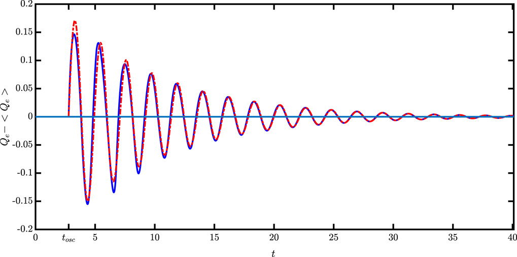
To confirm the validity of the theory, a number of tests have been performed. Two of them are presented in the following. The first analysis refers to the case shown in figure 1. The behaviour of $Q_{e}(t)$ , as obtained numerically with the shell method, has been fitted by a damped sinusoid $Q_{e}(t)\simeq A\sin (\unicode[STIX]{x1D6FA}_{0}t+\unicode[STIX]{x1D6FC})\exp (-\unicode[STIX]{x1D6E4}_{0}t)$ giving $\unicode[STIX]{x1D6FA}_{0}=2.9206$ and $\unicode[STIX]{x1D6E4}_{0}=0.1218$ . Then (3.33) has been solved numerically, starting from the trial value $\unicode[STIX]{x1D714}_{0}=\unicode[STIX]{x1D6FA}_{0}+\text{i}\unicode[STIX]{x1D6E4}_{0}$ , eventually giving $\unicode[STIX]{x1D714}=2.9139+\text{i}0.1237$ .

Figure 7.

Damped oscillations of the electron charge for the same case as figure 1 (full line), and best fit as $Q_{e}-\langle Q_{e}\rangle =A\sin (\unicode[STIX]{x1D6FA}_{0}t+\unicode[STIX]{x1D6FC})\exp (-\unicode[STIX]{x1D6E4}_{0}t)$ (dashed line); ( $\langle Q_{e}\rangle$ is the steady state for $Q_{e}$ , as given by (2.7)).

Another study is presented in figure 8. By considering a fixed value for the total charge of the system, $Q_{tot}$ , the steady state of $Q_{e}$ , obtained from (2.7), and the corresponding values from numerical solution with the shell method are reported for different values of $I_{0}$ (figure 8 a). When $I_{0}$ increases, there is a transition between damped and steady oscillations for the electron charge. For the same values of the parameters, the value of $\unicode[STIX]{x1D6E4}=\text{Im}(\unicode[STIX]{x1D714})$ is reported (figure 8 b). As can be noticed, the value of $I_{0}$ for the transition corresponds to the condition $\unicode[STIX]{x1D6E4}(I_{0})=0$ . In reality, equation (3.33) has a complicated set of eigenvalues $\unicode[STIX]{x1D714}$ . Here, only one has been calculated for each value of the electron flux $I_{0}$ with a simple procedure. For the smallest value of $I_{0}$ considered, for which the oscillations are damped, $\unicode[STIX]{x1D714}$ has been obtained as for the case in figure 7. Then, $I_{0}$ was increased by $\unicode[STIX]{x0394}I_{0}$ and the new $\unicode[STIX]{x1D714}$ was calculated numerically from (3.33) using the previous $\unicode[STIX]{x1D714}$ as a guess. Obtaining the full spectrum of $\unicode[STIX]{x1D714}^{\prime }$ was beyond the purposes of the present work.

4 Discussion and conclusive remarks

One may wonder why the system considered here shows an irreversible behaviour (in particular, the tendency towards a steady-state configuration), which is usually associated with collisional phenomena. In reality, there are well-known situations in which a collisionless plasma presents damped oscillations (e.g. Landau damping), however in the case studied in this paper the physical cause is completely different, as collisions do exist when the electrons are absorbed by the sphere. In this case, the information about their velocity is lost, and the only way to time revert the electron dynamics would be by reemitting electrons that are absorbed with the right velocity (i.e. the velocity when they hit the sphere), which is unknown after the collision. Also, the case of steady oscillations can be regarded as an irreversible behaviour, as it is a limit cycle, which is independent of the initial perturbation of the steady-state equilibrium. With reference to figure 4, it can be noticed that the initial velocity of the emitted electrons is a known quantity ( $v_{0}$ , a constant in the present model), but the velocity of the particles when they are absorbed is variable (it oscillates in time) as the electric potential is time dependent and the energy of a single particle is not a constant of the motion.

Figure 8.

(a) Electron charge $Q_{e}$ as a function of the flux $I_{0}$ for a fixed value of the total charge $Q_{0}=1$ , as given by system (2.8) (full line, red). Average electron charge after the transient (averaged over the oscillations), evaluated with the shell method, together with the maximum and the minimum values of $Q_{e}$ in a period of oscillation, as a function of $I_{0}$ (dots, blue). (b) Plot of $\unicode[STIX]{x1D6E4}=\text{Im}(\unicode[STIX]{x1D714})$ as a function of $I_{0}$ , for the same value of $Q_{tot}$ , obtained from (3.29)–(3.32).

As mentioned in the Introduction, the initial motivation for the present study was to investigate the possibility of calculating the equilibrium distribution of the electrons when the density of the positive charge is known. The answers of the present work are these:

1. (i) in every situation which is significant from a physical point of view (i.e. a non-negative charge on the sphere before the electron emission) a steady-state distribution for the electrons exists;

2. (ii) the solution either corresponds to a real stationary state (when the oscillations are damped) or it represents the mean value of the charge over an oscillation period. As the period is usually much smaller with respect to the characteristic time of the ion dynamics, also in the latter case the steady-state solution can be usefully employed.

In order to apply these methods to the original problem (i.e. plasma expansion in a vacuum in spherical geometry) two extensions are still necessary:

1. (i) to include the effect of the ion charge outside the sphere, which can be easily introduced into the equations; this can be done by suitably modifying (2.5), as

   (4.1) $$\begin{eqnarray}\displaystyle \left.\begin{array}{@{}l@{}}{\displaystyle \frac{\text{d}U}{\text{d}r}}={\displaystyle \frac{\unicode[STIX]{x1D6F9}_{e}+eQ_{i}}{r^{2}}},\\ {\displaystyle \frac{\text{d}\unicode[STIX]{x1D6F9}_{e}}{\text{d}r}}=-{\displaystyle \frac{2e^{2}I_{0}}{\left[\displaystyle \frac{2}{m}({\mathcal{E}}-U)\right]^{1/2}}},\end{array}\right\} & & \displaystyle\end{eqnarray}$$
   where $\unicode[STIX]{x1D6F9}_{e}(r)/er^{2}$ is the electric field due to the sphere and to the electrons, while $Q_{i}(r)$ is the ion charge in the region $[R,r]$ ; however, in general $U(r)$ may not be a monotonic function of $r$ , and, consequently, in these cases $U$ (or $p$ ) cannot be used as independent variables;

2. (ii) to consider the real velocity distribution (e.g. a Maxwellian) for the electrons when they are emitted. This last point can be dealt with by approximating the energy spectrum of the emitted electrons as a superposition of cold beams of different velocity. An alternative possibility is suitably adapting the ergodic method (Peano et al. Reference Peano, Peinetti, Mulas, Coppa and Silva2006) originally introduced to study the dynamics of nanoplasmas; this will be the object of future research.