1. Introduction
The mixing of scalars, such as temperature, chemical species and pollutants, in turbulent flows is a common phenomenon, e.g. pollutant dispersion (Vanderwel & Tavoularis Reference Vanderwel and Tavoularis2014), turbulent stratified flow (Caulfield Reference Caulfield2021) and combustion (Pope Reference Pope1991), and comprehensive reviews on this topic can be found in Warhaft (Reference Warhaft2000), Shraiman & Siggia (Reference Shraiman and Siggia2000), Dimotakis (Reference Dimotakis2005), Villermaux (Reference Villermaux2019) and Sreenivasan (Reference Sreenivasan2019). Mixing occurs when turbulent motion distorts surfaces/interfaces between fluids (Corrsin & Kistler Reference Corrsin and Kistler1955; Dimotakis, Miake-Lye & Papantoniou Reference Dimotakis, Miake-Lye and Papantoniou1983; Cetegen & Mohamad Reference Cetegen and Mohamad1993). The complexity of these surfaces/interfaces increases while mass flux transport is enhanced (Cetegen & Mohamad Reference Cetegen and Mohamad1993; Catrakis et al. Reference Catrakis, Aguirre, Ruiz-Plancarte, Thayne, McDonald and Hearn2002; Peltier & Caulfield Reference Peltier and Caulfield2003).
To quantify the geometric complexity of scalar interfaces, Mandelbrot (Reference Mandelbrot1975) employed the fractal dimension in a theoretical investigation of Gaussian random fields, which approximate Kolmogorov homogeneous turbulence. He proposed a fractal dimension
 $D_F=8/3$
for three-dimensional iso-scalar surfaces. In planar laser-induced fluorescence (PLIF) measurements of a turbulent jet flow, Prasad & Sreenivasan (Reference Prasad and Sreenivasan1990) obtained
 $D_F = 7/3$
for the interfaces between turbulent flow and quiescent ambient flow. Using the co-area formula from geometric measure theory (Federer Reference Federer1969) together with the first-order velocity structure function, Constantin, Procaccia & Sreenivasan (Reference Constantin, Procaccia and Sreenivasan1991) theoretically demonstrated that
 $D_F = 2+\zeta _1^{(u)}$
for iso-scalar turbulent/non-turbulent interfaces, and
 $D_F = 2.5+\zeta _1^{(u)}/2$
for iso-scalar surfaces in the inertial–convective range of turbulent flows. In Kolmogorov-type turbulence, turbulent kinetic energy cascades in the inertial range with a characteristic
 $-5/3$
scaling in the velocity spectrum, and the first-order structure function of velocity exhibits a power-law scaling with scaling exponent
 $\zeta _1^{(u)}=1/3$
. This gives
 $D_F = 2.67$
for three-dimensional iso-scalar surfaces in fully turbulent flows. In the same study, Constantin et al. (Reference Constantin, Procaccia and Sreenivasan1991)showed that
 $D_F = 1.67 \pm 0.04$
(
 $\approx 2.67-1$
) from a two-dimensional PLIF measurement in the passive scalar mixing of a turbulent jet, which agrees with their theoretical prediction based on the additive law (Mandelbrot Reference Mandelbrot1975). In addition, the fractal dimension
 $D_F=2.67$
manifests when the flow length scale is larger than a crossover scale (Constantin et al. Reference Constantin, Procaccia and Sreenivasan1991), below which the iso-scalar surfaces are smoother. The ratio of this crossover length scale to the Kolmogorov length scale is approximately
 $10$
, independent of the Reynolds number (Constantin et al. Reference Constantin, Procaccia and Sreenivasan1991). In another theoretical study, Grossmann & Lohse (Reference Grossmann and Lohse1994) also predicted fractal dimension
 $D_F = 2.67$
for iso-scalar surfaces in turbulence, based on geometric measure theory with the second-order velocity structure function and the Batchelor interpolation formula. They predicted that the crossover length scale is approximately
 $14$
times the Kolmogorov length scale. One point worth noting is that in theoretical studies, the criteria and thresholds determining iso-scalar surfaces are not discussed, given their ideal configuration in mathematics.
Experimental and numerical studies need to consider the criteria and thresholds to extract the iso-surfaces, and they show that the fractal dimension may vary with the thresholds, criteria and Reynolds number (Miller & Dimotakis Reference Miller and Dimotakis1991; Frederiksen, Dahm & Dowling Reference Frederiksen, Dahm and Dowling1996; Dasi, Schuerg & Webster Reference Dasi, Schuerg and Webster2007; Zubair & Catrakis Reference Zubair and Catrakis2009). For instance, the iso-scalar surfaces extracted with a relatively large threshold denote the passive scalars that are not well mixed by the turbulence, yet evolve into wrinkling surfaces presenting fractal features (Iyer et al. Reference Iyer, Schumacher, Sreenivasan and Yeung2020). Miller & Dimotakis (Reference Miller and Dimotakis1991) conducted an experiment to examine the fractal dimension of one-dimensional time iso-scalar surfaces of turbulent jets, with careful handling of noise. Contrary to expectations of a constant fractal dimension across the range of Reynolds numbers studied, the fractal dimension varied continuously from
 $0$
to
 $1$
, influenced by both the scales and the threshold values. Lane-Serff (Reference Lane-Serff1993) reported a threshold-dependent fractal dimension of iso-scalar surfaces in liquid-phase jet and plume flows in the far field, and the intensity threshold for surfaces was in the range
 $0.1$
–
 $1.1$
times the local mean. This gives a fractal dimension ranging from
 $D_F=1.23$
to
 $D_F = 1.60$
, yet reaching
 $D_F=1.67$
evidenced in the turbulent jet (Constantin et al. Reference Constantin, Procaccia and Sreenivasan1991). Villermaux & Innocenti (Reference Villermaux and Innocenti1999) conducted an experiment with the passive scalar continuously injected into a turbulent jet. They show that the fractal dimension of the iso-scalar surfaces (extracted with a criterion based on initial concentration) increases from approximately
 $1.13$
to approximately
 $1.3$
, then decreases along with the streamwise direction of the jet. Dasi et al. (Reference Dasi, Schuerg and Webster2007) studied the geometric properties of the iso-scalar surfaces for a point source of passive scalar releasing into the inertial layer of the turbulent boundary layer. They used the root mean square (RMS) of the scalar concentration as the criterion, and showed that the fractal dimension depends not only on the RMS thresholds, but also on the Reynolds number. From the same set-up, Mohaghar, Dasi & Webster (Reference Mohaghar, Dasi and Webster2020) later reported that the fractal dimension increases by approximately 1.1–1.5 along the jet, when the flow transits to fully developed turbulence. Iyer et al. (Reference Iyer, Schumacher, Sreenivasan and Yeung2020) performed direct numerical simulations (DNS) of the three-dimensional passive scalar mixing in homogeneous isotropic turbulence at
 $Sc=1$
. They used the scalar RMS as the criterion, and examined the fractal dimension within a range of the scalar RMS thresholds. They observed that the fractal dimension varied continuously with the thresholds, similar to the findings in Miller & Dimotakis (Reference Miller and Dimotakis1991), but with an upper bound
 $D_F=2.67$
in the inertial range (Iyer et al. Reference Iyer, Schumacher, Sreenivasan and Yeung2020). Recently, the fractal dimension
 $2.67$
was further confirmed by Gauding et al. (Reference Gauding, Thiesset, Varea and Danaila2022) through the two-point statistics of the phase indicator at large Reynolds numbers in the three-dimensional passive scalar mixing in homogeneous isotropic turbulence using the same numerical configuration as Iyer et al. (Reference Iyer, Schumacher, Sreenivasan and Yeung2020).
Most studies on the fractal dimension analysis of the iso-scalar surfaces focus on the inertial–convective range, where the dependence on the Schmidt number is limited. In the viscous–convective range, the scalar spectrum is expected in theory to display a
 $-1$
scaling (Batchelor Reference Batchelor1959; Kraichnan Reference Kraichnan1968; Sreenivasan Reference Sreenivasan2019), and the passive scalar mixing in turbulence greatly depends on the Schmidt number, for
 $Sc\gtrsim 1$
. In the theoretical study of Grossmann & Lohse (Reference Grossmann and Lohse1994), taking the relation between the Hausdorff dimension and the fractal dimension, they predict that the fractal dimension increases to be larger than
 $1.67$
to approach and saturate at
 $D_F=2$
for high Schmidt numbers (e.g.
 $Sc\gt 10^2$
; see their figure 1), as the scale decreases from the inertial–convective range. For further decrease of the scales, the fractal dimension is predicted to come to
 $D_F=1$
. In the experimental study of turbulent boundary layer flows, Dasi et al. (Reference Dasi, Schuerg and Webster2007) investigated the fractal dimension of the passive scalar mixing (
 $Sc\approx 1250$
), among the inertial–convective and viscous–convective ranges. They show that the fractal dimension increases up to
 $D_F=1.3$
, followed by a decrease, as the length scale decreases within the inertial–convective range and viscous–convective range, respectively. No sign of the plateaued
 $D_F$
is observed; see figure 8 in Dasi et al. (Reference Dasi, Schuerg and Webster2007). Recently, Iyer et al. (Reference Iyer, Schumacher, Sreenivasan and Yeung2020) observed
 $D_F\gt 1.67$
at the small scales (before decrease around the Kolmogorov scale), from their DNS at
 $Sc=1$
, in good agreement with the theoretical prediction of Grossmann & Lohse (Reference Grossmann and Lohse1994). For large Schmidt number mixing, the discrepancy between the theory and the observations remains.
The aforementioned studies have not yet reached an agreement on the fractal dimension in the turbulent passive scalar mixing. In particular, in the experiments, different criteria and thresholds are used in varieties of flow problems, and this complicates the findings and comparisons among studies. To clarify their influence on the measured fractal dimension, careful examinations need to be carried out on the same measurement results with various criteria and thresholds. Motivated by these questions and considerations, in this study, we investigate the fractal characteristics of the passive scalar mixing in turbulent pipe flow at
 ${Re}= 10\,000$
–
 $20\,000$
with Schmidt number
 $Sc\approx 2000$
, in both of the inertial–convective and viscous–convective ranges. Three commonly used criteria in the literature with correspondingly various thresholds are examined to explore their influence on the measured fractal dimension using the same data. The detailed descriptions of the experimental set-up and the PLIF measurements are introduced in § 2. Then the fractal features of the iso-scalar surfaces and discussion about the effects of the thresholds, criteria and Reynolds numbers on the fractal dimension are presented in § 3. Finally, the conclusion is drawn in § 4.
(a) A sketch of the experimental set-up for passive scalar turbulent mixing in turbulent pipe flow. The Cartesian coordinates are indicated by red arrows. (b) Illustration of the optical elements for the PLIF technique, including the beam expander and optical filter. (c) The laser intensity normalised by the ensemble average of its peaks, namely
 $\langle I_{{peak}}\rangle$
. The blue solid line represents the data from the photodetector (PDA100A2, Thorlabs) with sampling frequency 40 kHz, and the red circles indicate the mean value (
 $I_{\textit{mean}}$
) of a laser pulse.

2. Experimental methodology
2.1. Experimental set-up
The experiments were conducted in a straight rigid pipe with a circular cross-section. The working fluid is water. The entire set-up consists of a constant-head tank, polyvinyl chloride (PVC) tubes, a contraction nozzle, acrylic tubes, a dye injector, a refractive-index-matching box and an outlet tank, as sketched in figure 1(a). The constant-head tank, located
 $2$
m above the acrylic pipes, is separated into two portions: one portion serves as an overflow outlet and the collected water is reused as water supply, while the other maintains a constant level to achieve steady pressure to drive the fluid flow in the pipe. The PVC tubes, with inner diameter
 $72\pm0.1$
mm, connect the constant-head tank to the contraction nozzle. The 3-D-printed contraction nozzle (made of photosensitive resin) is designed with area contraction ratio
 $3.15$
to minimise perturbations from the upstream flow. The pipe is composed of four acrylic tubes with inner diameter
 $D=40 \pm 0.05$
mm, resulting in total length
 $4$
m (
 $100D$
dimensionless). The ends of each pipe segment were machined so that the four pipe segments could be seamlessly connected via Perspex connectors to minimise disturbances.
The dye injector is located
 $L_1=50D$
downstream from the nozzle. This length is sufficiently long for achieving fully developed turbulence in the pipe for the Reynolds number
 ${Re}\geqslant 10\,000$
considered here (White Reference White2016). The velocity profiles are examined via the particle image velocimetry (PIV) measurements, as described in Appendix A. Here,
 ${Re}$
is defined as
 $U_b D/\nu$
, where
 $U_b$
is the mean (or bulk) flow speed, and
 $\nu$
is the kinematic viscosity of the fluid. The dye injector system consists of three components: an L-shaped needle with inner diameter (
 $d$
) 2 mm and outer diameter 2.4 mm (much smaller than the pipe diameter
 $D=40$
mm), a gear pump for maintaining a continuous and constant flow rate, and a tank filled with the Rhodamine 6G solution in concentration
 $100\ \unicode{x03BC} \mathrm{g\ l^{-1}}$
, which is the initial concentration
 $\phi _0$
. The Schmidt number of the Rhodamine 6G solution,
 $Sc = \nu /\kappa$
where
 $\kappa$
is the molecular diffusivity of Rhodamine 6G in water, is approximately
 $2000$
. The L-shaped needle is positioned within a Perspex connector, and its exit aligns with the centre of the pipe to ensure that it matches the streamwise direction of the pipe flow. The injection velocity is kept constant and matched to the mean velocity of the pipe flow at the pipe centre.
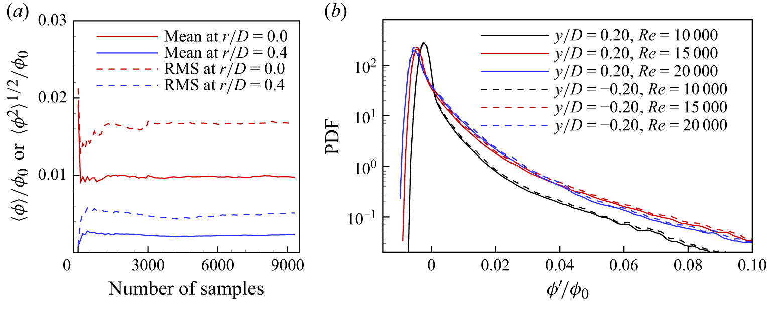
(a) Convergence test for the mean and RMS of the concentration field when
 ${Re}=20\,000$
. (b) The PDFs of the concentration fluctuations at symmetric positions for different
 ${Re}$
.

The measurements were conducted at
 $L_2=10D$
downstream of the exit of the needle injector. This distance is chosen to avoid the wake perturbation caused by the needle. The turbulence mixes and spreads the dye across the streamwise direction, but not so completely that the camera sensor can detect strong fluctuation of the fluorescence signal, in a good signal-to-noise ratio. The measurement field of view (FOV) is approximately
 $167d$
from the injector exit, so the injector is expected to have a trivial influence on the measurements (Villermaux & Innocenti Reference Villermaux and Innocenti1999). A part of the L-shaped injector is along the pipe radial direction, and is expected to generate wakes affecting the flows. To evaluate the influence, the probability density function (PDF) of the scalar concentration fluctuation (
 $\phi ^\prime$
) is plotted in figure 2(b). The PDFs from the positive and negative
 $y/D$
are nearly collapsed, and the statistics here are of symmetry to the pipe axis. This implies that the wake perturbation from the needle injector can be ignored, given that the initial injector wake is asymmetric to the pipe axis. A refractive-index-matching box, made of acrylic plates and filled with water, surrounds the pipe to reduce optical distortion caused by the differences in refractive indices among acrylic, water and air. The camera captures an image of a calibration plate of markers. This calibration plate consists of dots, which have diameter
 $0.5$
mm and are arranged in an equidistant lattice pattern with 2 mm spacing (van Doorne & Westerweel Reference van Doorne and Westerweel2007). This calibration obtains the conversion relationship between the image world and the physical world. A turbine flow meter and an electric ball valve were mounted in the disposal tube of the outlet tank, for controlling the flow rates. The experiments were conducted at three Reynolds numbers, 10 000, 15 000 and 20 000. The flow characteristics corresponding to these Reynolds numbers are summarised in table 1. The velocity characteristics are examined by the PIV measurements. The profiles of the velocity and the estimated Kolmogorov scale
 $\eta _K$
are presented in Appendix A as an example.
Summary of the flow characteristic parameters at the pipe centre. The Taylor microscale Reynolds number is given by
 $Re_\lambda = u_{{rms}} \lambda /\nu$
, where
 $u_{{rms}}$
is the RMS of the velocity fluctuations,
 $\lambda$
is the Taylor microscale, and
 $\nu$
is the kinetic viscosity. Here,
 $D$
is the diameter of the pipe and
 $d$
is the diameter of the injection needle. The Kolmogorov scale is
 $\eta _K = (\nu ^3/\epsilon )^{1/4}$
, with dissipation rate
 $\epsilon$
. The Kolmogorov time scale (
 $\tau _K$
) equals
 $\eta _K^2/\nu$
. The Batchelor scale is estimated by
 $\eta _B \approx \eta _K\,Sc^{-1/2}$
(Batchelor Reference Batchelor1959) with
 $Sc \approx 2000$
.

2.2. Measurement instrumentation
A Cartesian coordinate system is set with the origin at the exit of the needle injector (the centre of the pipe cross-section), while
 $z$
and
 $y$
are set along the pipe axis and pipe radial directions, respectively. The high-resolution PLIF technique is used to measure the passive scalar field, as illustrated schematically in figure 1(b). The light illumination is provided by a Beamtech Vlite-Hi-527 pulsed laser (Nd:YLF laser with wavelength 527 nm). For the experiments in this study, the laser was operated at 1 kHz, and the pulse duration is
 $200$
ns, which is sufficient to ‘freeze’ the scalar flow structures on the PLIF images, ensuring that the instantaneous state of the scalar field is accurately captured without motion blur on the images. A beam splitter is used to split the laser beam into two beams. One beam is used to create a laser sheet positioned in the vertical plane through the centreline of the pipe flow. The optics configuration for generating the laser sheet is carefully designed to achieve the thinnest sheet in the centre region of the pipe, optimising the resolution of the scalar field measurements. To achieve this, a beam expander is used to expand the laser diameter, and a reverse apodizing neutral density filter (NDYR20A, Thorlabs) is used to produce a laser beam with a near-Gaussian intensity profile. This expanded laser beam is then converted via a concave lens to a beam with diameter approximately 12 mm. Then a spherical convex lens (with focal length
 $300$
mm) and a cylindrical concave lens (with focal length
 $-25$
mm) are used to generate the laser sheet from the laser beam. The average thickness of the laser sheet within the radial measurement regions (
 $|y/D|\lt 0.4$
) is approximately 200
 $\unicode{x03BC}$
m, and the thinnest is approximately 7.0
 $\unicode{x03BC}$
m, at
 $y/D\approx 0$
(Ready Reference Ready1997; Crimaldi Reference Crimaldi2008), which is sufficient for spatially resolving the Kolmogorov length scale in the present experiments; see table 1.
The camera (PCO) used in this study is a 12-bit complementary metal oxide semiconductor (CMOS) camera with resolution
 $2016\times2016$
pixels
 $^2$
. To achieve the desired spatial resolution, an 85 mm macro lens is employed, resulting in approximate resolution 27
 $\unicode{x03BC}$
m pixel–1. This spatial resolution is smaller than the Kolmogorov length scale for Reynolds numbers ranging from 10 000 to 20 000, ensuring that the small turbulent structures are adequately resolved, as indicated in table 1. A long-pass filter with a 550 nm cut-off is mounted in front of the camera lens to block scattered light from the incoming laser and improve the quality of the PLIF measurements. It ensures that only the fluorescence signal is captured. The field of view covers area approximately
 $D \times 1.1D$
. Overall, this measurement configuration is carefully designed to particularly resolve scalar motions in the inertial–convective range, providing detailed insights into the turbulent mixing dynamics within this flow regime in this study.
The secondary beam from the beam splitter is detected by a photodetector (PDA100A2, Thorlabs) to monitor and record the laser intensity variations over time. A synchroniser is used to simultaneously trigger the laser, camera and photodetector, ensuring precise timing and synchronisation of data acquisition. The sampling rate for both laser and camera is 1 kHz, whereas the photodetector monitors the laser intensity at 40 kHz within each laser pulse, as shown in figure 1(c). This figure shows that the pulsed laser slightly fluctuates over time. To address these fluctuations and ensure accurate data, the mean laser intensity within each pulse (
 $I_{\textit{mean}}$
, represented by red symbols in figure 1(c), is used to correct the intensity of the PLIF images (
 $I_{{\textit{LIF},\,\textit{raw}}}$
), on the basis of the relationship
 \begin{equation} \frac {I_{{\textit{LIF},\,\textit{raw}}}}{I_{{\textit{LIF},\,revise}}} = \frac {I_{\textit{mean}}}{\left \langle I_{\textit{mean}}\right \rangle }, \end{equation}
where
 $\left \langle {\cdot }\right \rangle$
denotes the ensemble average operation. The corrected PLIF images (
 $I_{{\textit{LIF},\,revise}}$
), including calibration and measurement images, are subsequently used to calculate the concentration following the procedure described in Xu & Chen (Reference Xu and Chen2012). Note that this revision is based on the assumption that the intensity profile of a pulsed laser beam has relatively uniform and weak changes over operation time.
A total of 9300 images were captured for each Reynolds number. The tests for convergence are shown in figure 2(a), where the mean and RMS of the concentration field at
 $|y/D|=0.0$
and
 $|y/D|=0.4$
are shown to approach the corresponding constants as the number of samples increases, suggesting that 9300 samples are sufficient for the statistical convergence.
3. Results and discussion
3.1. Mean and fluctuating scalar fields
Some basic statistics of the scalar concentration fields are obtained and presented, with comparisons among similar independent studies. Figure 3(a) shows a snapshot of the concentration contours
 $\phi$
measured by PLIF at
 ${Re} = 10\,000$
. The profiles of the mean concentration
 $\langle \phi \rangle$
in the measurement region (i.e.
 $z/D = 10.7$
) are displayed in figure 3(b). These profiles are normalised by their respective peak concentrations. The mean profiles are well approximated by fitted Gaussian curves, which are shown as lines in the figure. In our experiment, the mean profile consistently exhibits a single peak. These findings are in agreement with those of Lavertu & Mydlarski (Reference Lavertu and Mydlarski2005) and Germaine, Mydlarski & Cortelezzi (Reference Germaine, Mydlarski and Cortelezzi2014). Similar trends in mean profiles have also been reported by Brethouwer et al. (Reference Brethouwer, Boersma, Pourquié and Nieuwstadt1999), Lavertu & Mydlarski (Reference Lavertu and Mydlarski2005) and Germaine et al. (Reference Germaine, Mydlarski and Cortelezzi2014). The widths of the mean profiles slightly increase with the increase of
 ${Re}$
. This observation may be attributed to the fact that the plume from the needle injector is stirred and spreads closer to the wall due to higher turbulent fluctuations at the larger Reynolds numbers. In our measurement region (
 $10.1\leqslant z/D\leqslant 11.2$
), the mean profiles show negligible changes over downstream positions, as shown in figure 3(c). Several examples of the spatial concentration profiles are presented in figure 3(d), where significant variations appear. A similar trend is also observed in the temporal concentration profiles shown in figure 3(e).
(a) A snapshot of the concentration by PLIF at
 ${Re} = 10\,000$
. Here,
 $\phi _0$
represents the initial concentration in the needle. (b) Mean concentration profiles normalised by their respective peak values (
 $\phi _{{peak}}$
) at the downstream location
 $z/D = 10.7$
for Reynolds numbers
 ${Re} = 10\,000$
(
 ),
 $Re=15\,000$
(
 ) and
 $Re=20\,000$
(
 ). The symbols indicate the profiles from the PLIF measurements, and the solid lines correspond to the best-fit Gaussian profiles, where approximately every other ten points are shown for clarity. (c) Mean concentration profiles normalised by their respective peak values (
 $\phi _{{peak}}$
) at different downstream locations for
 ${Re} = 20\,000$
and
 $z/D = 10.2$
(
 ),
 $z/D = 10.7$
(),
 $z/D = 11.2$
(
 ). (d) Space signals of the concentration at the pipe centre at
 $t = 10D/U_b$
(black),
 $20D/U_b$
(red),
 $30D/U_b$
(cyan) for
 ${Re} = 20\,000$
. (e) Time signals of the concentration at
 $(y/D,z/D)=(0.2,10.2)$
(black),
 $(y/D,z/D)=(0.2,10.7)$
(red) and
 $(y/D,z/D)=(0.2,11.2)$
(cyan) for
 ${Re} = 15\,000$
. ( f) The PDFs of the scalar fluctuations at radial locations
 $|y/D| = 0, 0.2, 0.4$
for different Reynolds numbers (
 ${Re}=10\,000, 15\,000, 20\,000$
), where the line patterns correspond to the Reynolds numbers, and the colours indicate different radii. The inset shows the PDFs around their peaks.

The PDFs of the concentration fluctuations
 $\phi '$
at different radial positions (
 $|y/D|$
) are shown in figure 3( f) at downstream position
 $z/D =10.7$
for the three Reynolds numbers. All PDFs are spiked and skewed. As
 ${Re}$
increases or the radial position decreases, the width of the PDFs increases and their peaks decrease, as shown in the inset of figure 3( f). The decreasing tails of the PDFs at
 $|y/D| = 0$
(blue lines in the figure) exhibit an approximate power-law shape, which is independent of
 ${Re}$
, as discussed in Villermaux, Innocenti & Duplat (Reference Villermaux, Innocenti and Duplat2001). Similar PDF profiles have been reported in Lavertu & Mydlarski (Reference Lavertu and Mydlarski2005), Lepore & Mydlarski (Reference Lepore and Mydlarski2011) and Germaine et al. (Reference Germaine, Mydlarski and Cortelezzi2014) for thermal plumes. However, other tails depend on the position and
 ${Re}$
(especially close to the wall, e.g. at
 $|y/D| = 0.40$
, black lines in figure 3
f), which may be related to the inhomogeneity of the turbulent pipe flow, and needs further investigation. The statistical results of the high-resolution PLIF measurements are similar to those of previous studies, indicating the good quality of our measurements. Therefore, according to the above results, the present streamwise measurement region
 $10.1 \leqslant z/D \leqslant 11.2$
is used for the subsequent analysis of the fractal dimension of the iso-scalar surfaces.
3.2. Fractal dimension in the inertial–convective range
Studies have demonstrated that the geometry of iso-scalar surfaces in turbulent scalar fields can be characterised in terms of the fractal dimension (Prasad & Sreenivasan Reference Prasad and Sreenivasan1990; Constantin et al. Reference Constantin, Procaccia and Sreenivasan1991; Catrakis & Dimotakis Reference Catrakis and Dimotakis1996; Dasi et al. Reference Dasi, Schuerg and Webster2007; Iyer et al. Reference Iyer, Schumacher, Sreenivasan and Yeung2020). To analyse the fractal properties of the mixing scalar surfaces, the box-counting method is employed in this study. This method has been widely used in many studies of the fractal geometry of iso-scalar surfaces (e.g. Prasad & Sreenivasan Reference Prasad and Sreenivasan1990; Constantin et al. Reference Constantin, Procaccia and Sreenivasan1991; de Silva et al. Reference de Silva, Philip, Chauhan, Meneveau and Marusic2013; Mistry et al. Reference Mistry, Philip, Dawson and Marusic2016). In the box-counting method, the number of boxes, which the iso-scalar surfaces pass through, scales with the box size
 $r_b$
as
 $N(r_b) \sim r_b^{-D_F}$
, where
 $D_F$
is the fractal dimension (Mandelbrot Reference Mandelbrot1982; Sreenivasan Reference Sreenivasan1991).
Sample concentration fields
 $\phi /\phi _0$
at
 ${Re}=20\,000$
. The colour bar is the same as that in figure 3(a). The concentration contours serving as the background and iso-scalar surfaces at different thresholds are marked as solid cyan lines: (a)
 $\phi_{th}=1.0\langle \phi \rangle$
, (b)
 $\phi_{th}=2.0\langle \phi \rangle$
, (c)
 $\phi_{th}=3.0\langle \phi \rangle$
, (d)
 $\phi_{th}=4.0\langle \phi \rangle$
. See supplementary movie 1 at https://doi.org/10.1017/jfm.2025.10454.

Coverage count of boxes
 $\langle N\rangle /(D/\eta _K)$
required to cover different iso-scalar surfaces versus box size
 $r_b/\eta _K$
(and
 $r_b/D$
) and corresponding fractal dimensions (
 $D_F$
) at different thresholds: (a,d)
 ${Re}=10\,000$
, (b,e)
 ${Re}=15\,000$
, (c,f)
 ${Re}=20\,000$
. The grey dashed line in (d–f) denotes
 $D_F=1.67$
. Magenta arrows indicate the Taylor microscales (plain arrow) and the integral length scale (hollow arrow) at
 $|y/D|=0$
. Black arrows indicate correspondingly the same scales at
 $|y/D| = 0.4$
. (Note that the integral scale at
 $|y/D| = 0.4$
is underestimated due to the limited streamwise measurement field of view, within which the autocorrelation of the streamwise velocity does not yet reach zero.) Taylor microscales and integral length scales at
 $0\lt |y/D|\lt 0.4$
lie in between those at
 $|y/D|=0$
and
 $|y/D|=0.4$
. These arrow symbols have the same meanings in later figures.

The ensemble average of the concentration field over time,
 $\langle \phi \rangle$
, is taken as the criterion, and the thresholds
 $\phi _{{th}}/\langle \phi \rangle = 1.0{-}4.0$
are used to extract the iso-scalar surfaces of the scalar concentration fields. In figures 4(a–d), a sample of the concentration contours of
 $\phi /\phi _0$
is served as the background, and the iso-scalar surfaces with different thresholds are shown as solid cyan lines. At
 $\phi _{{th}} = 1.0\langle \phi \rangle$
, the edges of the mixing structures are detected; however, the experimental noise is also captured, as shown close to the borders of figure 4(a). As
 $\phi _{{th}}$
increases, the regions where the concentration is closer to the initial concentration are enclosed by the isolines, e.g. see the bright yellow regions in figures 4(b–d), where significant mixing does not occur.
Furthermore, the box-counting method is applied to the iso-scalar surfaces at different thresholds. The coverage count
 $\langle N\rangle$
of boxes, after ensemble averaging over all measured fields (de Silva et al. Reference de Silva, Philip, Chauhan, Meneveau and Marusic2013), is plotted in figures 5(a–c) on log-log axes for three Reynolds numbers, namely 10 000, 15 000 and 20 000. Here,
 $\langle N\rangle$
decreases as the normalised scale
 $r_b/\eta _K$
increases, where
 $\eta _K$
is the Kolmogorov length scale in the pipe centre. (The Kolmogorov length scale in the pipe centre
 $\eta _K$
is used for the normalisation, in consistency with the Kolmogorov scale used for the later fractal dimensions of one-dimensional space data along the pipe axis in § 3.4. Here, the fractal dimension is obtained over the two-dimensional iso-scalar surfaces; the corresponding Kolmogorov scale for normalisation is not straightforward, given that the Kolmogorov scale has a profile along the pipe radius. Since the fractional statistics are taken mostly for
 $|y/D|\lt 0.4$
(see figure 4), and the larger thresholds closer to the pipe centre, the average Kolmogorov scale weighted by the mean concentration is
 $\overline {\eta }_K = [\int _0^{D/2} \langle \phi \rangle \eta _K\,\mathrm{d}y]/[\int _0^{D/2} \langle \phi \rangle\, \mathrm{d}y]\approx 0.93\eta _K$
, and a trivial shift along the horizontal axis is expected in the plots.) With different thresholds (
 $0.5 \leqslant \phi _{{th}}/\langle \phi \rangle \leqslant 4$
),
 $\langle N\rangle$
decreases as the thresholds increase over a small scale range (approximately
 $r_b/\eta _K \lt 10$
), where the scaling gradually approaches
 $-1$
as
 $\phi _{{th}}/\langle \phi \rangle$
is increased from
 $0.5$
to
 $4$
. Conversely, for the scale range
 $r_b/\eta _K \gt 10$
,
 $\langle N\rangle$
does not vary significantly among
 $\phi _{{th}}/\langle \phi \rangle$
values, visually approaching the scaling
 $1.67$
.
(a) Plot of
 $D_F$
(with the additive law) of one-dimensional
 $\phi$
along the streamwise direction at
 $|y/D|=0.3$
. (b) Plot of
 $D_F$
of one-dimensional
 $\phi$
with threshold
 $1.0\langle \phi \rangle$
, along the radial (
 $y$
) direction (averaged over streamwise locations) and along the streamwise direction at five
 $|y/D|$
values. In (a) and (b),
 ${Re}= 10\,000$
and the grey dashed line denotes
 $D_F=1.67$
. See the caption of figure 5 for the meanings of the arrows.

For better examining the scaling, the fractal dimension
 $D_F$
of the fractal level sets is computed via the equation
 \begin{equation} D_F = -\frac {\mathrm{d}\!\left[\mathrm{log}\left [\left \langle N\right \rangle /(D/\eta _K)\right ]\right]}{\mathrm{d}\!\left[\mathrm{log}(r_b/\eta _K)\right]}. \end{equation}
Figures 5(d–f) present the fractal dimension for the iso-scalar surfaces of the scalar fields, corresponding to the
 $\langle N\rangle$
–
 $r_b$
plots in figures 5(a–c), respectively. The convergence tests of the number of samples are detailed in Appendix B. As illustrated in figures 5(d–f), the fractal dimension for a threshold
 $\phi _{{th}}$
increases continuously over the small scale range, reaching
 $D_F\gt 1.67$
, followed by a gradual decrease to approach a nearly constant
 $1.67\pm 0.05$
, when
 $r_b/\eta _K$
locates in the inertial–convective range. The uncertainty (
 $\pm 0.05$
) arises from the curve fitting
 $\langle N\rangle$
–
 $r_b$
for
 $r_b/\eta _K\gt 10$
, as suggested in Constantin et al. (Reference Constantin, Procaccia and Sreenivasan1991). The uncertainty of the curve fitting decreases as the fitting region beyond
 $r_b/\eta _K\gt 10$
narrows. Although the iso-scalar surfaces with the threshold
 $\phi _{{th}}/\langle \phi \rangle = 1.0$
are contaminated by experimental noise near the wall region (see figure 4
a), this noise has minimal impact on this fractal dimension (
 $1.67\pm 0.05$
). Additionally, to further evaluate the fractal dimension, the one-dimensional
 $\phi$
at various radial positions
 $|y/D|$
along the pipe axis is taken to calculate the fractal dimension
 $D_F$
with the additive law (Mandelbrot Reference Mandelbrot1982). As shown in figure 6(a), the fractal dimension in the inertial–convective range is approximately
 $1.67$
and is approximately unaffected by the thresholds shown here. Across different radial positions,
 $D_F$
is approximately
 $1.67$
within the inertial–convective range; see figure 6(b). Overall, for the three Reynolds numbers considered in the present study, the fractal dimension in the inertial–convective range is approximately
 $1.67$
, which within the margin of error is in good agreement with the values from experiments with the turbulent jet flow (Constantin et al. Reference Constantin, Procaccia and Sreenivasan1991) and theoretical studies (Mandelbrot Reference Mandelbrot1975; Constantin et al. Reference Constantin, Procaccia and Sreenivasan1991; Grossmann & Lohse Reference Grossmann and Lohse1994).
Whether the quality of
 $D_F = 1.67$
is affected by the thresholds is under considerable debate (see e.g. the discussions in Miller & Dimotakis Reference Miller and Dimotakis1991; Lane-Serff Reference Lane-Serff1993; Villermaux & Innocenti Reference Villermaux and Innocenti1999; Iyer et al. Reference Iyer, Schumacher, Sreenivasan and Yeung2020). To explore this,
 $D_F$
as a function of the threshold is shown in figure 7, where the thresholds (
 $\phi _{{th}}$
) ranging from
 $0.01 \langle \phi \rangle$
to
 $8 \langle \phi \rangle$
are selected. The fractal dimension was obtained from the linear fits of the coverage count in the log-log plots (e.g. figure 5
a) for
 $r_b/\eta _K \gt 10$
. In figure 7, as the threshold increases,
 $D_F$
decreases but a clear plateau (approximately 1.67) can be observed for
 $0.5 \lesssim \phi _{{th}}/\langle \phi \rangle \lesssim 3.5$
. These results are consistent with those of previous experimental studies (Lane-Serff Reference Lane-Serff1993) and DNS studies (Iyer et al. Reference Iyer, Schumacher, Sreenivasan and Yeung2020). When the threshold is smaller (
 $\phi _{{th}}\lt 0.5\langle \phi \rangle$
), the fractal dimension is larger than the value in the plateau, which can be attributed to the measurement noise in the iso-scalar surfaces. As shown in figure 4(a) and discussed earlier, the measurement noise contaminates the iso-scalar surfaces, resulting in an increase in the coverage count of the boxes, and thus affecting the quality of the power-law scaling. Finally, a high fractal dimension is obtained. For the cases with larger thresholds (
 $\phi _{{th}}\gt 4\langle \phi \rangle$
), the extracted iso-scalar surfaces are within the less mixed regions. As illustrated in figure 4(d), the iso-scalar surfaces are located in regions with high concentration values, leading to smoother surfaces and consequently a smaller
 $D_F$
. This result makes physical sense. Fluorescent dye with high scalar concentration values is continuously injected into the pipe flow, moving downstream at a finite velocity and being stirred by the fluctuation velocity field (turbulent eddies) of the ambient turbulent flow. This process disperses the dye in all directions, leading to connected and disconnected filaments with sharp borders. When the threshold is relatively low, the borders of the filaments are extracted exactly where mixing occurs, exhibiting fractal characteristics. However, as the threshold becomes large, the scalar concentration within the filament does not mix with the ambient turbulent flow, preventing the development of a wrinkled and fractal surface (Iyer et al. Reference Iyer, Schumacher, Sreenivasan and Yeung2020).
The fractal dimension as a function of the threshold (
 $\phi _{{th}}/\langle \phi \rangle$
) for the iso-scalar surfaces in the measurement region. The grey dashed line denotes
 $D_F=1.67$
, and the two grey dash-dotted lines mark the range of
 $\phi _{{th}}/\langle \phi \rangle$
, within which
 $D_F\approx 1.67$
.

Previous studies have employed different criteria to extract iso-scalar surfaces (see e.g. Villermaux & Innocenti Reference Villermaux and Innocenti1999; Dasi et al. Reference Dasi, Schuerg and Webster2007; Iyer et al. Reference Iyer, Schumacher, Sreenivasan and Yeung2020). To evaluate the impact of these criteria on the fractal dimension, two other criteria, which are commonly used in the aforementioned studies, are used to extract the iso-scalar surfaces, as shown in figures 8(b,c). The first criterion uses
 $m$
times the local RMS above the local mean (
 $\phi _{{th}} = \left \langle \phi \right \rangle + m \phi _{{rms}}$
(e.g. Dasi et al. Reference Dasi, Schuerg and Webster2007; Iyer et al. Reference Iyer, Schumacher, Sreenivasan and Yeung2020), and the second criterion uses
 $m$
times the initial concentration (
 $\phi _{{th}} = m \phi _0$
), which is also equivalent to using a constant value as the threshold (e.g. Prasad & Sreenivasan Reference Prasad and Sreenivasan1990; Villermaux & Innocenti Reference Villermaux and Innocenti1999; de Silva et al. Reference de Silva, Philip, Chauhan, Meneveau and Marusic2013; Zhuang et al. Reference Zhuang, Tan, Huang, Liu and Zhang2018; Mohaghar et al. Reference Mohaghar, Dasi and Webster2020). The iso-scalar surfaces determined by the first criterion exhibit a pattern of filaments similar to those obtained using
 $m$
times the local mean when the threshold values are close; see figures 8(a) and 8(b). When the thresholds are similar, minimal differences are observed between the resulting mixing iso-scalar surfaces. In contrast, the criterion using the initial concentration (constant) retains the mixing surfaces at the centre of the pipe flow; see figure 8(c). The box-counting method is applied to the iso-scalar surfaces using these two criteria to obtain the coverage count of the boxes. As shown in figures 9(a,c), for the range of small scales,
 $\langle N \rangle$
decreases with the increase of the threshold, and approaching the
 $-1$
scaling. For larger scales, as
 $r_b/\eta _K$
increases, the decrease of
 $\langle N\rangle$
approaches to follow a corresponding scaling. For clarity, the corresponding
 $D_F$
over large scales (
 $r_b/\eta _K \gt 20$
), the saturated scalings, are presented in figures 9(b,d). A plateau
 $D_F \approx 1.67$
over a range of thresholds can be observed. These tests clearly demonstrate that although the choice of criteria can influence the details of the extracted iso-scalar surfaces, the general trend of fractal dimension scaling remains consistent, and a constant fractal dimension within a certain range of thresholds can be obtained. This consistency reinforces that the fractal dimension is a reliable descriptor of the complexity of iso-scalar surfaces in turbulent pipe flow of passive scalar mixing, validating both theoretical predictions and experimental observations in turbulent environments (Constantin et al. Reference Constantin, Procaccia and Sreenivasan1991).
It should be mentioned that similar experiments of passive scalar mixing in an open-channel turbulent boundary layer show a low fractal dimension; see Dasi et al. (Reference Dasi, Schuerg and Webster2007). Their experiments showed less dense concentration fields with fewer iso-scalar flow structures, possibly due to the lower turbulence intensity from the background turbulence, leading to a limited number of filament structures observed in one image for the box-counting method. In contrast, in our experiments, the initially homogeneous fluid with dye from the injection system is stretched and swirled by the turbulence in pipe flow. As a result, the core with a high concentration is partially preserved, while clear fluid is entrained into the core, and the dye fluid is folded to generate filaments. The number of filaments observed in our experiments is greater than that observed in Dasi et al. (Reference Dasi, Schuerg and Webster2007), which statistically increases the coverage count for the box-counting method. This demonstrates the presence of multiscale structures of mixing iso-scalar surfaces deformed by turbulent eddies.
An instantaneous sample of iso-scalar surfaces with different criteria when
 ${Re}=20\,000$
: (a)
 $\phi _{{th}}=4.0\langle \phi \rangle \in [0.59, 5.02]$
, (b)
 $\phi _{{th}}=\langle \phi \rangle + 2\phi _{{rms}} \in [0.31, 4.88]$
, (c)
 $\phi _{{th}}=0.04\phi _0 = 4$
. The unit of
 $\phi _{{th}}$
is
 $\unicode{x03BC}$
g l–1.

Box-counting results for iso-scalar surfaces are shown for two threshold criteria when
 ${Re}=20\,000$
: (a,b)
 $m$
times the local RMS above the local mean, specifically,
 $\phi _{{th}} = \langle \phi \rangle + m \phi _{{rms}}$
; (c,d)
 $m$
times the initial concentration, namely
 $\phi _{{th}} = m \phi _0$
. (a,c) The number of boxes required to cover iso-scalar surfaces with different thresholds versus box size
 $r_b/\eta _K$
. The fractal dimension
 $D_F = 1.67$
at large scales is represented by the dashed line, whereas
 $D_F = 1$
at small scales is represented by the dash-dotted line. (b,d) Fractal dimension
 $D_F$
as a function of the threshold, where the grey dashed line indicates
 $D_F=1.67$
. See the caption of figure 5 for the meanings of the arrows.

The fractal dimension
 $D_F\approx 1.35$
characterises the turbulent/non–turbulent interfaces in turbulent jet flows, where the ambient flow remains quiescent, and entrainment occurs at the interfaces (Prasad & Sreenivasan Reference Prasad and Sreenivasan1990; Mistry et al. Reference Mistry, Philip, Dawson and Marusic2016, Reference Mistry, Dawson and Kerstein2018). The fractal dimension agrees with the theoretical predictions of Prasad & Sreenivasan (Reference Prasad and Sreenivasan1990) and Constantin et al. (Reference Constantin, Procaccia and Sreenivasan1991). Recent investigations have demonstrated that the fractal dimension of turbulent/non-turbulent interfaces is influenced by the applied threshold at low turbulence intensities, yielding values at approximately 2.1 (below the typical 2.35) in three-dimensional measurements (e.g. Er, Laval & Vassilicos Reference Er, Laval and Vassilicos2023; Zhang, Watanabe & Nagata Reference Zhang, Watanabe and Nagata2023). Similarly, other studies have also shown that the fractal dimension of interfaces between a turbulent ambient flow and a turbulent jet increases with the turbulence intensity of the ambient flow (e.g. Kankanwadi & Buxton Reference Kankanwadi and Buxton2020; Kohan & Gaskin Reference Kohan and Gaskin2022; Chen & Buxton Reference Chen and Buxton2023). Thus the presence of background turbulence can notably affect the fractal dimension of the mixing surfaces because the turbulent eddies can stir the mixing parcel and generate a mixing and wrinkling surface. In the present study, the flow emerging from the injection needle exhibits jet-like characteristics, yet the surrounding flow is a fully developed turbulent pipe flow. In the far field of the injection needle (approximately
 $220d$
downstream), active and well-developed mixing can be seen in the current measurement. There are no obvious entrainment interfaces between the ambient flow (pipe flow) and jet flow (from the needle), as mixing structures still exist in the region close to the wall, even with a high threshold; see figure 4(d). The present experimental conditions match better with the condition that the theories of fractal dimension consider for the iso-scalar surface in the passive scalar mixing (Constantin et al. Reference Constantin, Procaccia and Sreenivasan1991). Therefore, the fractal dimension
 $D_F \approx 1.35$
for the turbulent/non–turbulent interfaces is not observed in this study. Instead, the iso-scalar surfaces of the mixing structures in this study tend towards fractal dimension
 $1.67$
in the turbulence (Constantin et al. Reference Constantin, Procaccia and Sreenivasan1991).
3.3. Critical crossover length scale
(a) An illustration of extracting the crossover length scale from the
 $\langle N \rangle{-}r_b$
plot (
 ${Re}=20\,000$
). (b) The ratio
 $r^*/\eta _K$
from different studies of the passive scalar mixing. (c) The crossover length scale determined using the second-order structure function of velocity increments. (d) The ratio
 $r^*/\eta _K$
obtained from the second-order velocity structure function (open symbols) and velocity spectra (half-filled symbols). The ratio of
 $r^{**}$
to
 $r^*$
versus
 ${Re}_\lambda$
is shown in the inset of (b). Here,
 ${Re}_\lambda$
in Constantin et al. (Reference Constantin, Procaccia and Sreenivasan1991) is evaluated as
 $Re_\lambda \approx \sqrt {2{Re}}$
(Pope Reference Pope2000). In the legends, ATBL refers to the atmospheric turbulent boundary layer, TBL denotes the turbulent boundary layer, HIT denotes homogeneous isotropic turbulence, and TSF denotes turbulent swirling flow. See the caption of figure 5 for the meanings of the arrows.

In the theory proposed by Constantin et al. (Reference Constantin, Procaccia and Sreenivasan1991), a crossover length scale, denoted as
 $r^*$
, represents the transition between smooth surfaces at small scales and fractal surfaces at larger scales. Constantin et al. (Reference Constantin, Procaccia and Sreenivasan1991) predicted that the ratio
 $r^*/\eta _K$
is independent of the Reynolds number, suggesting a universal value. Grossmann & Lohse (Reference Grossmann and Lohse1993) supported this prediction and estimated the ratio to be approximately
 $10$
, the crossover length scale of the two distinct regimes of the scaling in the second-order structure function of velocity increments.
This crossover length scale is examined in this study. The method for estimating
 $r^*$
is illustrated in figure 10(a). The log-log plot of the coverage count
 $\langle N\rangle$
of boxes of size
 $r_b/\eta _K$
is divided into two parts: the left part (for
 $-0.3\lt \mathrm{log_{10}}(r_b/\eta _K) \lt 0.5$
) and the right part (for
 $\mathrm{log_{10}}(r_b/\eta _K)\gt 1.7$
). The left and right parts are linearly fitted, with the latter having slope
 $-1.67$
. Thresholds ranging from
 $2.0 \langle \phi \rangle$
to
 $4.0\langle \phi \rangle$
in 0.5 increments are used. The average and standard deviation of the crossover length scales across different thresholds provide the value and error bar, respectively. Our results, shown in figure 10(b), indicate that the critical crossover length scale is approximately 10 times the Kolmogorov scale. The results from studies of Constantin et al. (Reference Constantin, Procaccia and Sreenivasan1991) and Iyer et al. (Reference Iyer, Schumacher, Sreenivasan and Yeung2020) were extracted using the same method, and are shown in figure 10(b) with different colour symbols. The
 $r^*/\eta _K$
value in this study exhibits a slight increase with the increase of
 ${Re}$
, similar to the value of Constantin et al. (Reference Constantin, Procaccia and Sreenivasan1991) in a jet with a slightly larger Reynolds number, and smaller than the values of Iyer et al. (Reference Iyer, Schumacher, Sreenivasan and Yeung2020) in a homogeneous isotropic turbulence, which has much larger
 ${Re}_\lambda$
.
Moreover, according to Grossmann & Lohse (Reference Grossmann and Lohse1993), the ratio
 $r^*/\eta _K$
marks the transition from the viscous range to the inertial range, where fluid motion appears fractal. Grossmann & Lohse (Reference Grossmann and Lohse1993) observed this ratio in the second-order structure function of velocity increments, namely,
 $S_2(r) = \langle [u^\prime (r+z)-u^\prime (z)]^2\rangle = \langle [\Delta u^\prime (r)]^2 \rangle$
, where
 $\Delta u^\prime (r)$
denotes the velocity difference over a distance
 $r$
along the
 $z$
direction. In the present study, the longitudinal second-order structure functions are plotted in figure 10(c). From the two known scalings, i.e.
 $S_2(r)\sim r^2$
and
 $S_2(r)\sim r^{2/3}$
(Pope Reference Pope2000), their intersection gives a crossover length scale
 $r^{**}/\eta _K$
, shown in figure 10(d) as black symbols. The
 $r^{**}/\eta _K$
values of other experimental studies from their second-order velocity structure function (van Atta & Chen Reference van Atta and Chen1970; Antonia, Satyaprakash & Hussain Reference Antonia, Satyaprakash and Hussain1980; Mestayer Reference Mestayer1982; Anselmet et al. Reference Anselmet, Gagne, Hopfinger and Antonia1984) and the velocity spectra (Debue et al. Reference Debue, Kuzzay, Saw, Daviaud, Dubrulle, Canet, Rossetto and Wschebor2018) are shown in figure 10(d), in addition to the theoretical predictions (Effinger & Grossmann Reference Effinger and Grossmann1987; Zhang et al. Reference Zhang, Bodenschatz, Xu and Xi2021) and experimental collections (Pope Reference Pope2000). Our results are consistent with their results, indicating that the crossover length scale is approximately 10 times the Kolmogorov scale.
The inset of figure 10(b) shows that the ratio of
 $r^*/\eta _K$
(from the scalar fractal surfaces) and
 $r^{**}/\eta _K$
(from the velocity structure function) is approximately
 $1$
, in good agreement with the theoretical prediction of Grossmann & Lohse (Reference Grossmann and Lohse1993). This comparison demonstrates that the geometric complexity of iso-scalar surfaces is intricately linked to the dynamics of turbulent mixing.
3.4. Fractal dimension in the viscous–convective range
Given by the geometric measure theory, the scaling behaviour of the Hausdorff volume
 $H$
of a passive scalar graph over a three-dimensional ball
 $B_r$
with radius
 $r$
is given by
 $H(g(B_r)) \sim r^{D_g}$
, where
 $g$
is the graph over the sphere. The scaling dimension of the graph,
 $D_g$
, is connected to the fractal dimension by
 $D_F = D_g -1$
(Iyer et al. Reference Iyer, Schumacher, Sreenivasan and Yeung2020); see details in Grossmann & Lohse (Reference Grossmann and Lohse1994), Eckhardt & Schumacher (Reference Eckhardt and Schumacher1999) and Iyer et al. (Reference Iyer, Schumacher, Sreenivasan and Yeung2020). Theoretical predictions of the fractal dimension
 $D_F$
(Grossmann & Lohse Reference Grossmann and Lohse1994) at
 $Sc=1$
and
 $2000$
are shown in figure 11; meanwhile, the
 $D_F$
of the DNS with
 $Sc = 1$
from Iyer et al. (Reference Iyer, Schumacher, Sreenivasan and Yeung2020) is extracted from their figure and shown as symbol lines.
The fractal dimension
 $D_F$
versus
 $r_b/\eta _K$
(and
 $r_b/\eta _B$
). The data are obtained from two-dimensional PLIF images for
 ${Re}=10\,000$
(squares) with threshold
 $0.5\langle \phi \rangle$
, and the data points are skipped for clarify. The fractal dimensions predicted by the geometric measure theory model (
 $D_g$
) (Grossmann & Lohse Reference Grossmann and Lohse1994) and DNS (Iyer et al. Reference Iyer, Schumacher, Sreenivasan and Yeung2020) are shown using a relationship
 $D_F = D_g - 1$
with the additive law. The inset shows
 $D_F$
with thresholds
 $0.5\langle \phi \rangle$
–
 $3\langle \phi \rangle$
. See the caption of figure 5 for the meanings of the arrows.

Since
 $D_F$
is independent of the Reynolds numbers in this study (see figure 5),
 $D_F$
at
 ${Re}=10\,000$
is shown in figure 11, where the spatial and temporal resolutions are most close to resolving the small-scale motions. When the box size
 $r_b$
is very small, the iso-scalar field exhibits smoothness, i.e.
 $D_F\approx 1$
. As
 $r_b$
increases,
 $D_F$
increases gradually to reach a maximum
 $D_F\approx 1.85$
at
 $r_b/\eta _K \approx 7$
, where the iso-scalar surfaces are wrinkled. For further larger length scales, the passive scalar field manifests the fractality
 $D_F \approx 1.67$
; see figure 11. Albeit that the fractal dimension indicates ‘wrinkled’ iso-scalar surfaces at some small scales, as predicted for
 $Sc\gtrsim 1$
from the theory of Grossmann & Lohse (Reference Grossmann and Lohse1994), this curve is close to the prediction for
 $Sc=1$
, much smaller than the prediction for
 $Sc=2000$
(Grossmann & Lohse Reference Grossmann and Lohse1994); see the black solid line in figure 11. The
 $D_F$
value is obtained from the two-dimensional scalar field. The averaged resolution of the scalar measurements is approximately
 $35\eta _B$
in space and approximately 0.016
 $\tau _K$
in time, where
 $\tau _K$
is the Kolmogorov time scale. The measurements insufficiently resolve the flow motions in the viscous–convective range; correspondingly, the averaging effect of the camera pixel gives smoothed scalar signals, leading to smaller
 $D_F$
. Based on this analysis, the one-dimensional
 $\phi$
at a single pixel (
 $y/D=0$
) along the pipe axis is taken to obtain the fractal dimension
 $D_F$
with the additive law (Mandelbrot Reference Mandelbrot1982). Along this spatial line, the resolution is approximately
 $5\eta _B$
within the measurement plane, and approximately
 $\eta _B$
in the depth direction of the laser sheet, close to the Batchelor scale. This
 $D_F$
is shown as the in figure 12(a), which agrees with the theoretical curve of Grossmann & Lohse (Reference Grossmann and Lohse1994) for
 $Sc=2000$
. With a larger threshold, i.e.
 $0.2\langle \phi \rangle$
,
 $D_F$
still shows
 $D_F\approx 2$
for
 $1\lesssim r_b/\eta _K \lesssim 5$
, but gets smaller for
 $r_b/\eta _K \lt 1$
, as shown in figure 12(b). The agreement of the measured
 $D_F$
from the one-dimensional space
 $\phi (y/D=0)$
with the theoretical curve of Grossmann & Lohse (Reference Grossmann and Lohse1994) remains for the criteria of
 $\phi _{{rms}}$
and
 $\phi _{0}$
, as shown in figure 12(c).
(a) The fractal dimension
 $D_F$
(with the additive law) of one-dimensional spatial PLIF results at
 $y/D = 0$
versus
 $r_b/\eta _K$
(and
 $r_b/\eta _B$
) with threshold
 $0.05\langle \phi \rangle$
. The lines denote the prediction of Grossmann & Lohse (Reference Grossmann and Lohse1994). (b) The
 $D_F$
values from the same spatial sequence with different thresholds of
 $\langle \phi \rangle$
. (c) The
 $D_F$
values from the same spatial sequence with different criteria. The data points are skipped for clarity.

To further evidence the influence of the resolution on the fractal dimension, two test cases were considered for one-dimensional data from
 $\phi (y/D=0)$
at
 ${Re}=10\,000$
. In the first case, the data are sub-sampled with skipping size
 $\varDelta _s \approx 0.2\eta _K$
. In the second case, the data are filtered with a box filter of size
 $\varDelta \approx 0.2\eta _K$
, followed by sub-sampling the filtered sequence with skipping
 $\varDelta _s=\varDelta$
points. This operation mimics the PLIF measurements by a camera sensor with a coarser spatial resolution, given that a pixel of a camera sensor works like a box for collecting the light. In figure 12(a), the
 $D_F$
value of the sub-sampled sequence (denoted by the pink hollow squares) remains consistent with that of the raw sequence, which indicates that the constant
 $D_F$
persists in accordance with the definition of the fractal (box-counting) dimension. The
 $D_F$
value from the sequence with
 $\varDelta \approx 0.2\eta _K$
and
 $\varDelta _s\approx 0.2\eta _K$
is smaller than that from the raw sequence in the viscous–convective range, but is unchanged in the inertial–convective range. With a larger filter size (
 $\varDelta \approx 0.3\eta _K$
and
 $\varDelta _s\approx 0.3\eta _K$
),
 $D_F$
in the viscous–convective range decreases further, and a monotonic increase of
 $D_F$
with
 $r_b/\eta _K$
can be observed. This demonstrates that the fractal dimension at the small scales is particularly sensitive to the measurement resolution and measurement quality. This is one possible technical cause for the fractal dimension
 $D_F\approx 2$
in the viscous–convective range being overlooked in previous experiments.
4. Conclusion
In this study, we present the geometric analysis of passive scalar mixing in turbulent pipe flow at Reynolds numbers 10 000, 15 000 and 20 000. The high-resolution PLIF technique was used to measure the passive scalar concentration field at a high sampling rate, so that the Kolmogorov scales are well resolved in our measurements. The scalar field is characterised by the mean concentration profiles and PDFs along the radial direction. These statistics are in agreement with those reported by Lavertu & Mydlarski (Reference Lavertu and Mydlarski2005) and Lepore & Mydlarski (Reference Lepore and Mydlarski2011), justifying the measurements.
The fractal dimension of iso-scalar surfaces of the passive scalar mixing is obtained using the box-counting method. Three commonly used criteria for extracting the iso-scalar surfaces are examined to elucidate their effects on the fractal dimension analysis. The results from all three criteria demonstrate the fractal geometry characteristics in pipe flows, among a range of thresholds, given by fractal dimension
 $D_F = 1.67 \pm 0.05$
for length scales located in the inertial–convective range, independent of the Reynolds numbers. This is in good agreement with the theoretical predictions of Constantin et al. (Reference Constantin, Procaccia and Sreenivasan1991) and Grossmann & Lohse (Reference Grossmann and Lohse1994), and the numerical results of Gauding et al. (Reference Gauding, Thiesset, Varea and Danaila2022). The crossover length scale, the smaller end of the scale range where the fractal dimension
 $D_F\approx 1.67$
is observed, is found to be approximately 10 times the Kolmogorov scale, consistent with the theoretical predictions and former studies. In addition, the crossover length scales from the second-order velocity structure function are also examined. The ratio of the crossover length scales from the fractal dimension and the structure function is approximately unity, independent of the Reynolds numbers considered in this study. When the criterion threshold is large, there is less mixing of the core of scalar filaments, which has little likelihood of developing contortions of the iso-scalar surfaces, as discussed in Iyer et al. (Reference Iyer, Schumacher, Sreenivasan and Yeung2020).
In the viscous–convective range, the fractal dimension from the two-dimensional box-counting method (
 $D_F\gt 1.67$
) shows the sign of more ‘wrinkled’ iso-scalar surfaces than those in the inertial–convective range. However, this measured fractal dimension is smaller than the theoretical prediction of Grossmann & Lohse (Reference Grossmann and Lohse1994) for Schmidt number
 $2000$
. We show that this is possibly due to the fact that the two-dimensional measurements have insufficient resolutions for the Batchelor scales. When taking into consideration the one-dimensional scalar data along the pipe axis, where the spatial resolution is closer to the Batchelor scale, the fractal dimension is
 $D_F\approx 2$
with the additive law, in agreement with the prediction of Grossmann & Lohse (Reference Grossmann and Lohse1994). The theoretical prediction of Grossmann & Lohse (Reference Grossmann and Lohse1994) for the high Schmidt number scalar mixing is first evidenced in the experiment, to the best of our knowledge.
The passive scalar mixing is a transient process in general. The released scalar consists of filaments initially, evolves and diffuses in the flow over time, and finally ends up with a uniform distribution in space. In the pipe flow, the passive scalar is mixed by the turbulence; accordingly, the fractal dimension is expected to change along the streamwise direction and fatally to the smooth field. In this study, the measurements were taken arbitrarily
 $220d$
downstream from the dye injector, mainly from the measurement considerations – the wake perturbation of the injector is trivial while the camera sensor can capture strong scalar fluctuations with a good signal-to-noise ratio. This measurement helps to evidence the characteristic fractal dimension of iso-scalar surfaces in the inertial and viscous ranges, in general agreement with the theoretical predictions. Investigating the passive scalar mixing characteristics, including the corresponding fractal dimension, along the streamwise direction over a wide range is a rational choice and important for the coming study to better understand the nature of the mixing in shear flows. The scale separation for the moderate Reynolds numbers in this study is not distinct, and a larger Reynolds number flow is desirably necessary in the future study to examine the observations reported here. For a (very) large Reynolds number, the further smaller Batchelor scale is more challenging to be measured, and improvements on measurement techniques of the scalar concentration are required.
Supplementary movie
Supplementary movie is available at https://doi.org/10.1017/jfm.2025.10454
Acknowledgements
H.L. would like to acknowledge experimental support from Ms H. Liu and discussion from Dr T. Wu and Mr L. Wang. H.L. would also like to thank Professor E. Villermaux and Professor P. Orlandi for their questions and discussion during the 1st European Fluid Dynamics Conference, which helped us to prepare a better paper.
Funding
This work was supported by the National Natural Science Foundation of China (nos 11988102 and 92152106) and the China Postdoctoral Science Foundation (2023M733589).
Declaration of interests
The authors report no conflicts of interest.
Data availability statement
The data that support the findings of this study are available from the corresponding author upon reasonable request.
Author contributions
H.L. designed and performed the experiments, analysed the data, prepared the figures and wrote the main manuscript. D.X. conceptualised the study, guided the experiments, wrote the main manuscript and reviewed the manuscript. G.H. discussed the analysis, and wrote and reviewed the manuscript.
Appendix A. The PIV measurement configuration and flow velocity characteristics
For the same measurement field of view, the PIV measurements were carried out with the same high-speed camera and optical configuration as those in the PLIF measurements. The optical lenses were adjusted to generate the laser sheet of approximately
 $1$
mm thickness. Hollow glass spheres with medium diameter approximately
 $11$
 $\unicode{x03BC}$
m were used as the tracers. A multi-step correlation algorithm, implemented in the Lavision Davis software, was used to extract the displacement field. The interrogation window size at the final step was set to 32 pixels
 $\times$
32 pixels with a 50 % overlap. The image sampling rate was adjusted for each flow Reynolds number to ensure that the maximum displacement ranged from 6 to 8 pixels, adhering to the recommended one-quarter displacement within the window (Raffel et al. Reference Raffel, Willert, Scarano, Kähler, Wereley and Kompenhans2018). Approximately 20 000 snapshots of the PIV velocity fields were captured for each Reynolds number, providing sufficient data for statistical convergence in estimating the Kolmogorov scale and the second-order structure function of the velocity increments.
The flow characteristics are obtained in the PIV measurements. The Taylor microscale Reynolds number is estimated using
 $Re_\lambda = u_{{rms}} \lambda /\nu$
, where
 $u_{{rms}}$
is the RMS of the velocity fluctuations,
 $\lambda$
is the Taylor microscale, estimated from the two-point correlation of the streamwise velocity (Pope Reference Pope2000; Mohaghar et al. Reference Mohaghar, Dasi and Webster2020), and
 $\nu$
is the kinetic viscosity of fluid. At the pipe centre,
 ${Re}_{\lambda }=52.6$
,
 $67.5$
and
 $78.2$
, respectively, as shown in table 1. The dissipation rate
 $\epsilon$
is estimated using the two-dimensional PIV data with assumptions of isotropy, local isotropy, and local axisymmetry (Pope Reference Pope2000; Doron et al. Reference Doron, Bertuccioli, Katz and Osborn2001; Xu & Chen Reference Xu and Chen2013). The estimated dissipation rates from the three methods are very close, and their average is used to estimate the Kolmogorov length scale
 $\eta _K = (\nu ^3/\epsilon )^{1/4}$
.
Flow characteristics for the present experiments are shown in figure 13. In figure 13(a), the profiles of the mean streamwise velocity are presented for different
 ${Re}$
. These profiles show a good collapse with the profile from Eggels et al. (Reference Eggels, Unger, Weiss, Westerweel, Adrian, Friedrich and Nieuwstadt1994). The turbulence intensity profiles for different
 ${Re}$
along the radius of the pipe are shown in figure 13(b), together with profiles from El Khoury et al. (Reference El Khoury, Schlatter, Noorani, Fischer, Brethouwer and Johansson2013), and they agree well. The Kolmogorov scales
 $\eta _K$
are shown in figures 13(c) and 13(d). The estimated Kolmogorov length scales are close to the values reported in Bailey et al. (Reference Bailey, Hultmark, Schumacher, Yakhot and Smits2009) and Cerbus et al. (Reference Cerbus, Liu, Gioia and Chakraborty2020)at the pipe centre for the corresponding Reynolds numbers, marked as triangle symbols. The relative difference between the Kolmogorov scales among the profiles for
 $10.2\leqslant z/D \leqslant 11.2$
is less than 2 %.
Flow characteristic parameters along the radius: (a) mean streamwise velocity profiles (symbols), compared with the profile from Eggels et al. (Reference Eggels, Unger, Weiss, Westerweel, Adrian, Friedrich and Nieuwstadt1994); (b) the profiles of the turbulence intensity
 $u_{{rms}}/U_b$
, compared with the profiles from El Khoury et al. (Reference El Khoury, Schlatter, Noorani, Fischer, Brethouwer and Johansson2013); (c) Kolmogorov length scales
 $\eta _K$
, where the triangle symbols, coloured to match the corresponding lines, represent the values from Bailey et al. (Reference Bailey, Hultmark, Schumacher, Yakhot and Smits2009) and Cerbus et al. (Reference Cerbus, Liu, Gioia and Chakraborty2020) for the corresponding Reynolds numbers; (d)
 $\eta _K$
for
 ${Re}=20\,000$
at three streamwise positions.

Convergence test of the fractal dimension with threshold
 $4.0\langle \phi \rangle$
when
 ${Re}=15\,000$
. The symbols correspond to the number of samples. The grey dashed line indicates
 $D_F=1.67$
.

Appendix B. Convergence tests of number of samples for the box-counting method
The convergence test of the fractal dimension is shown in figure 14. As the number of samples exceeds 6000, the curves representing the fractal dimension become independent of the number of samples. This indicates that the variations in the fractal dimension with respect to the number of samples are minimal beyond this point. Therefore, the total number of 9300 samples used in this study is considered to be sufficient to achieve statistical convergence for fractal dimension analysis. This ensures the reliability of the fractal dimension results presented in our study.