1 Introduction
Fluid systems that are governed by multiple physical processes often exhibit instabilities that are composed of a complex interplay of many or all prevailing amplification and propagation mechanisms. Tonal noise about an aerofoil falls into this category, as convective hydrodynamic instabilities in both the pressure- and suction-boundary layers interact with acoustic waves radiating upstream from the trailing edge, which in turn retrigger the boundary layer instabilities, and in doing so sustain distinct pressure sound levels and select discrete frequencies via subtle feedback loops. Due to their very nature, the analysis of such instabilities requires a global (rather than local) point of view, since neither component in isolation – hydrodynamic or acoustic – can fully capture the tonal noise mechanism. An analysis of this type has been reported in Fosas de Pando, Schmid & Sipp (Reference Fosas de Pando, Schmid and Sipp2014) where the full global spectrum has been presented. The results of this study, including the global spectrum of the mean-flow-based linear operator, has shown that only a rather small number of global modes has a significant acoustic footprint to explain experimentally observed sound pressure levels and frequencies. The same study could identify and classify the shape and structure of flow patterns responsible for noise generation.
Equally important for a full understanding of tonal aerofoil noise is the quest for the origin of the acoustically active instabilities; in other words, we seek flow field structures (in type and location) that most efficiently trigger and sustain the noise-generating global modes. Adjoint methodology (Hill Reference Hill1995; Luchini & Bottaro Reference Luchini and Bottaro2014) will be used to furnish sensitivity information for these modes, and a pointwise superposition of local sensitivity measures (contained in the adjoint structure) and local amplification rates (contained in the direct/modal structure) will point towards positions in the flow field that act as so-called wavemakers. These positions optimally exploit both the responsiveness and the growth of global structures, and hence can be thought of as the source or origin of a global instability. Analyses of this type, also referred to as structural stability (see, e.g. Giannetti & Luchini Reference Giannetti and Luchini2007; Marquet, Sipp & Jacquin Reference Marquet, Sipp and Jacquin2008), have previously been applied to flows with simpler transport processes, where respective regions of amplification and sensitivity are convectively linked (Bottaro, Corbett & Luchini Reference Bottaro, Corbett and Luchini2003; Chomaz Reference Chomaz2005). Here, a more complex situation has to be addressed since flow information can be transported hydrodynamically and acoustically, and the full feedback loop consists of both components.
The tonal noise phenomenon on aerofoils, the focus of this study, has been investigated both experimentally and numerically over the past decades, starting with the experimental work of Paterson et al. (Reference Paterson, Vogt, Fink and Much1973) which led to an empirical expression for the dominant tonal frequency as a function of the Reynolds number. This was followed by an identification of multiple frequency peaks (see, e.g. Arbey & Bataille Reference Arbey and Bataille1983) and a resulting ladder structure as the free-stream velocity is varied. The multi-peak structure has been confirmed in further experiments as well as in numerical simulations by, for instance, Desquesnes, Terracol & Sagaut (Reference Desquesnes, Terracol and Sagaut2007), Jones & Sandberg (Reference Jones and Sandberg2011), Fosas de Pando et al. (Reference Fosas de Pando, Schmid and Sipp2014) and has been linked to feedback loops consisting of boundary layer instabilities and acoustic radiation. Simplified theoretical models – relying on a phase condition between local spatial growth, acoustic scattering on the trailing edge and a receptivity process at a prescribed location – have been proposed by Kingan & Pearse (Reference Kingan and Pearse2009), which reproduced well the observed frequencies for the tonal noise problem. A recent experimental study (Pröbsting, Serpieri & Scarano Reference Pröbsting, Serpieri and Scarano2014) has presented detailed time-resolved particle-image-velocimetry (PIV) measurements of acoustic sources near the trailing edge of the aerofoil, reporting that vortical structures, emanating from boundary layer instabilities, pass the trailing edge at the frequency of the dominant tone. Even though these vortical structures have been identified as one component of the tonal-noise generation mechanism, a full closed-loop analysis was beyond the experimental measurements. In the same study, a crucial involvement of the pressure side has also been suggested. Already early experimental work (Paterson et al. Reference Paterson, Vogt, Fink and Much1973) has similarly highlighted a characteristic sensitivity of acoustic tones on the details of aerofoil’s pressure-surface boundary layer.
The goal of the current study is then to use numerical simulations and adjoint techniques to extract, isolate and quantitatively describe the regions and structures of the flow that are principally responsible for the production of tonal noise. It aims at providing evidence and support for previous models, empiricisms and measurements. While the identification of noise-generating structures near the trailing edge has been the subject of various previous investigations, the current study shall not focus on this issue, but rather concentrate on the full (global) feedback loop consisting of multiple hydrodynamic instabilities, noise generation and propagation, and boundary layer receptivities to acoustic forcing. The article is organised as follows. After a description of the flow configuration and the numerical set-up (§ 2), which also contains a brief introduction to the adjoint analysis and the wavemaker argument, the global spectrum will be dissected (in § 3) into acoustically active modes (responsible for the acoustic tones) and the rather quiet high-frequency and low-frequency modes. Each type will be analysed as to its degree of sensitivity and its wavemaker location, and appropriate means for the passive or active manipulation of these modes will be suggested. The conclusions in § 4 give a summary and a complete structural description of tonal noise generation in flow about an aerofoil.
2 Flow configuration and numerical set-up
We take a numerical approach to the receptivity and sensitivity analysis of aerofoil tonal noise, consisting of a modal decomposition of the linearised governing equation, together with an accompanying analysis of the adjoint operator. A brief introduction to the principles of this type of analysis is given below.
2.1 Compressible Navier–Stokes numerical solver
We base our analysis on numerical simulations of the compressible Navier–Stokes equations on curvilinear structured grids using a pseudo-characteristics formulation (Sesterhenn Reference Sesterhenn2000). After proper non-dimensionalisation, the governing equations are discretised in space using high-order compact schemes: a fifth-order compact-upwind low-dissipative scheme (Adams & Shariff Reference Adams and Shariff1996) for the advective terms, and a third-order centred scheme (Lele Reference Lele1992) for the diffusive terms. Characteristics-based boundary conditions (Poinsot & Lele Reference Poinsot and Lele1992; Lodato, Domingo & Vervisch Reference Lodato, Domingo and Vervisch2008) are implemented, and non-reflecting inlet and outlet conditions at the computational domain are augmented by sponge layers to further attenuate spurious reflections (Bodony Reference Bodony2006). At this point, the governing equations consist of a system of ordinary differential equations of the form
 $$\begin{eqnarray}\frac{\text{d}\boldsymbol{v}}{\text{d}t}=\boldsymbol{F}(\boldsymbol{v}),\end{eqnarray}$$
which has to be integrated in time. In the above expression,
 $\boldsymbol{F}(\boldsymbol{v})$
denotes the nonlinear function representing the spatially discretised governing equations, and
 $\boldsymbol{v}$
stands for a composite vector containing the dependent flow variables (pressure
 $p$
, entropy
 $s$
and velocity vector
 $\boldsymbol{u}$
) at every grid point. For further details on the numerical solver, the reader is referred to Fosas de Pando et al. (Reference Fosas de Pando, Schmid and Sipp2014).
2.2 Evaluation of the linearised operators
Our study focuses on the dynamics of infinitesimally small perturbations superimposed on a reference flow field. To this end, we set
 $\boldsymbol{v}(t)=\overline{\boldsymbol{v}}+\boldsymbol{v}^{\prime }(t)$
in (2.1) and, upon linearisation, arrive at
 $$\begin{eqnarray}\frac{\text{d}\boldsymbol{v}^{\prime }(t)}{\text{d}t}=\unicode[STIX]{x1D63C}(\overline{\boldsymbol{v}})\boldsymbol{v}^{\prime }(t),\quad \text{with}~\unicode[STIX]{x1D63C}(\overline{\boldsymbol{v}})=\left.\frac{\unicode[STIX]{x2202}\boldsymbol{F}}{\unicode[STIX]{x2202}\boldsymbol{v}}\right|_{\overline{\boldsymbol{v}}},\end{eqnarray}$$
where
 $\unicode[STIX]{x1D63C}(\overline{\boldsymbol{v}})$
is referred to as the direct operator. In what follows, we will concentrate on the perturbation dynamics and omit the primes.
While the analysis of the direct operator provides pertinent information on the flow dynamics and instability mechanisms, even more valuable information can be obtained by accessing the associated adjoint operator, denoted by
 $\unicode[STIX]{x1D63C}^{\ast }$
. This operator is defined by the duality relation
 $\langle \boldsymbol{w},\unicode[STIX]{x1D63C}\boldsymbol{v}\rangle =\langle \unicode[STIX]{x1D63C}^{\ast }\boldsymbol{w},\boldsymbol{v}\rangle$
, where the inner product reads
 $\langle \boldsymbol{w},\boldsymbol{v}\rangle =\boldsymbol{w}^{H}\unicode[STIX]{x1D648}\boldsymbol{v}$
with
 $\unicode[STIX]{x1D648}$
as a Hermitian, positive definite weight matrix. Throughout this study, we choose the inner product
 $\langle \boldsymbol{w},\boldsymbol{v}\rangle$
based on the small-perturbation energy norm derived in Chu (Reference Chu1965) and Hanifi, Schmid & Henningson (Reference Hanifi, Schmid and Henningson1996) for compressible flows.
We stress that we consider the discrete adjoint, i.e. the adjoint of the discretised equations; for this reason, the above duality relation is satisfied up to machine precision. Based on this fundamental relationship and our specific choice of inner product, the operator
 $\unicode[STIX]{x1D63C}^{\ast }$
can be easily expressed in terms of the transconjugate of the direct operator
 $\unicode[STIX]{x1D63C}^{H}$
given by
 $\unicode[STIX]{x1D63C}^{\ast }=\unicode[STIX]{x1D648}^{-1}\unicode[STIX]{x1D63C}^{H}\unicode[STIX]{x1D648}$
. The numerical implementation of both linear operators
 $\unicode[STIX]{x1D63C}$
and
 $\unicode[STIX]{x1D63C}^{\ast }$
can conveniently be performed in matrix-free form using the methodology described in Fosas de Pando, Sipp & Schmid (Reference Fosas de Pando, Sipp and Schmid2012); in this reference, algorithms are described for the evaluation of the matrix-vector products
 $\unicode[STIX]{x1D63C}(\overline{\boldsymbol{v}})\boldsymbol{v}$
and
 $\unicode[STIX]{x1D63C}^{\ast }(\overline{\boldsymbol{v}})\boldsymbol{w}$
, directly from the implementation of the right-hand side in (2.1). This form of access to the linear operators is preferred over explicit storage of the direct operator
 $\unicode[STIX]{x1D63C}$
, since, for typical numbers of degrees of freedom and our choice of spatial discretisation, storage requirements well exceed typical memory resources.
2.3 Direct and adjoint global modes and computational details
We next turn our attention to the eigenvalue spectra of the direct operator
 $\unicode[STIX]{x1D63C}$
and its adjoint
 $\unicode[STIX]{x1D63C}^{\ast }$
. Starting from a modal decomposition for the perturbations in the form
 $\boldsymbol{v}_{k}\exp (-\text{i}\unicode[STIX]{x1D714}_{k}t)$
, we arrive at the eigenvalue problem given by
 $$\begin{eqnarray}-\text{i}\unicode[STIX]{x1D714}_{k}\boldsymbol{v}_{k}=\unicode[STIX]{x1D63C}\boldsymbol{v}_{k},\end{eqnarray}$$
with
 $\boldsymbol{v}_{k}$
as the direct global mode and
 $\unicode[STIX]{x1D714}_{k}=\unicode[STIX]{x1D714}_{r,k}+\text{i}\unicode[STIX]{x1D714}_{i,k}$
as the corresponding complex global frequency. Analogously, for each direct global mode, the associated adjoint global mode
 $\boldsymbol{w}_{k}$
is given by the eigenvalue problem
 $$\begin{eqnarray}\text{i}\unicode[STIX]{x1D714}_{k}^{\ast }\boldsymbol{w}_{k}=\unicode[STIX]{x1D63C}^{\ast }\boldsymbol{w}_{k},\end{eqnarray}$$
with
 $\unicode[STIX]{x1D714}_{k}^{\ast }=\unicode[STIX]{x1D714}_{r,k}-\text{i}\unicode[STIX]{x1D714}_{i,k},$
i.e. the complex conjugate eigenvalue of the direct problem (2.3). From the duality relationship, it is readily deduced that direct modes
 $\boldsymbol{v}_{k}$
and adjoint modes
 $\boldsymbol{w}_{l}$
are mutually bi-orthogonal unless
 $k=l$
. The direct and adjoint global modes are defined up to a multiplicative constant; hereinafter, all direct modes are normalised according to
 $\Vert \boldsymbol{v}_{k}\Vert ^{2}=1$
, and the associated adjoint global modes are rescaled such that
 $\langle \boldsymbol{w}_{k},\boldsymbol{v}_{k}\rangle =1$
. Numerically, the large-scale eigenvalue problems (2.3) and (2.4) are solved using the open-source software SLEPc (Hernández, Román & Vidal Reference Hernández, Román and Vidal2005) interfaced to our compressible simulation code. More specifically, a Krylov–Schur technique has been applied to the evolution operators
 $\exp (\unicode[STIX]{x0394}t\unicode[STIX]{x1D63C})$
and
 $\exp (\unicode[STIX]{x0394}t\unicode[STIX]{x1D63C}^{\ast })$
, which represent the time advancement over one time step
 $\unicode[STIX]{x0394}t$
by the direct or adjoint operator, respectively. The Krylov subspace is spanned by 2048 vectors, and the time step has been chosen as
 $\unicode[STIX]{x0394}t=0.015$
. Once a number of direct-adjoint eigenpairs has been computed, the degree of convergence is measured using the relative residuals given by
 $\Vert \unicode[STIX]{x1D63C}\boldsymbol{v}_{k}+\text{i}\unicode[STIX]{x1D714}_{k}\boldsymbol{v}_{k}\Vert _{2}/\Vert \unicode[STIX]{x1D714}_{k}\boldsymbol{v}_{k}\Vert _{2}$
and
 $\Vert \unicode[STIX]{x1D63C}^{\ast }\boldsymbol{w}_{k}-\text{i}\unicode[STIX]{x1D714}_{k}^{\ast }\boldsymbol{w}_{k}\Vert _{2}/\Vert \unicode[STIX]{x1D714}_{k}^{\ast }\boldsymbol{w}_{k}\Vert _{2}$
. In contrast to Fosas de Pando et al. (Reference Fosas de Pando, Schmid and Sipp2014), we do not employ a harmonic extraction technique, which yields lower relative residuals.
2.4 Wavemaker analysis
The direct global modes and the corresponding adjoint modes determine the structural sensitivity of the linearised operator
 $\unicode[STIX]{x1D63C}$
(Hill Reference Hill1992; Bottaro et al.
Reference Bottaro, Corbett and Luchini2003; Chomaz Reference Chomaz2005; Giannetti & Luchini Reference Giannetti and Luchini2007; Marquet et al.
Reference Marquet, Sipp and Jacquin2008). The sensitivity of the eigenvalues to perturbations in the operator
 $\unicode[STIX]{x1D63C}$
can be assessed by considering the perturbed eigenvalue problem
 $(\unicode[STIX]{x1D63C}+\unicode[STIX]{x1D6FF}\unicode[STIX]{x1D63C})(\boldsymbol{v}_{k}+\unicode[STIX]{x1D6FF}\boldsymbol{v}_{k})=-\text{i}(\unicode[STIX]{x1D714}_{k}+\unicode[STIX]{x1D6FF}\unicode[STIX]{x1D714}_{k})(\boldsymbol{v}_{k}+\unicode[STIX]{x1D6FF}\boldsymbol{v}_{k})$
and retaining only first-order terms. By computing the inner product of either side of the equation with the adjoint mode, we obtain
 $-\text{i}\unicode[STIX]{x1D6FF}\unicode[STIX]{x1D714}_{k}=\langle \boldsymbol{w}_{k},\unicode[STIX]{x1D6FF}\unicode[STIX]{x1D63C}\boldsymbol{v}_{k}\rangle$
. This latter expression indicates that the effect of a unitary proportional feedback between flow variables at different locations on any eigenvalue can be quantified by the scalar product between the adjoint at the output location and the direct global mode at the input location. We note that in general the feedback affects many eigenvalues of the matrix
 $\unicode[STIX]{x1D63C}$
. For the case of a diagonal operator perturbation
 $\unicode[STIX]{x1D6FF}\unicode[STIX]{x1D63C}$
, we restrict ourselves to a local feedback between each individual component at its given location. This approach leads to the concept of a wavemaker: the structural sensitivity of the flow to local (in-place) feedback quantified by the entrywise (Hadamard) product of the direct global mode and the corresponding adjoint global mode at a given location.
2.5 Flow configuration and parameters
We reconsider the flow case analysed in Fosas de Pando et al. (Reference Fosas de Pando, Schmid and Sipp2014) but, for the sake of completeness, provide a brief summary of the flow configuration and selected parameters. We compute the compressible flow about a NACA 0012 aerofoil section, at a two-degree angle of attack, with a sharp trailing edge. The chord-based Reynolds number
 $\mathit{Re}_{c}$
is taken as
 $2\times 10^{5}$
and the Mach number
 $\mathit{M}$
is 0.4. The specific heat ratio
 $\unicode[STIX]{x1D6FE}$
and the Prandtl number
 $\mathit{Pr}$
have been chosen as 1.4 and 0.71, respectively. Two-dimensional nonlinear simulations reveal that the flow reaches a quasi-periodic state characterised by vortices shedding into the wake and by a pressure spectrum in the far-field that is dominated by distinct tones at equally-spaced frequencies. The corresponding non-dimensional values for the dominant angular frequencies are
 $\unicode[STIX]{x1D714}\approx 37.02$
,
 $\unicode[STIX]{x1D714}\approx 39.47$
,
 $\unicode[STIX]{x1D714}\approx 41.93$
and
 $\unicode[STIX]{x1D714}\approx 44.38$
.
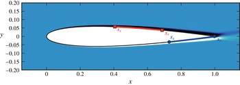
Proceeding with our analysis, the compressible Navier–Stokes equations are then linearised around the time-averaged flow field, depicted in figure 1 by the mean streamwise velocity component. This mean flow presents spatially-growing boundary layers on both aerofoil surfaces, with flow separation on both sides: the boundary layer detaches on the suction surface between
 $x_{s}\approx 0.405$
and
 $x_{r}\approx 0.686$
with a maximum reverse flow of 7 %, while on the pressure surface the mean flow detaches between
 $x_{s}\approx 0.728$
and
 $x_{r}\approx 0.977$
with a maximum reverse flow of 10 %.
Mean flow considered in the present study, visualised by the streamwise velocity component. The boundary layer on the suction surface detaches between
 $x_{s}\approx 0.405$
and
 $x_{r}\approx 0.686$
, while the pressure-surface boundary layer detaches between
 $x_{s}\approx 0.728$
and
 $x_{r}\approx 0.977$
. The reader is referred to Fosas de Pando et al. (Reference Fosas de Pando, Schmid and Sipp2014) for further details on the mean-flow characteristics.

3 Receptivity and sensitivity analysis
A study of the receptivity and sensitivity of tonal noise generation around an aerofoil must commence with the analysis of the global spectrum. Specifically, we will classify the modal structures according to their frequencies and the dominance of their physical components, and particular attention shall be directed towards the pressure component (or their dilatation field) as it indicates the acoustic footprint of the associated modal structure. In a second step then, the corresponding adjoint modes are computed which will furnish valuable information about the region of strongest sensitivity of the flow to a particular modal structure and the region of strongest localised (in-place) feedback; this latter analysis will point towards the spatial origin of a particular instability mechanism and guide possible (active or passive) control efforts.
3.1 Features of the global spectrum
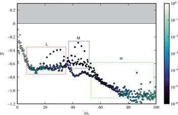
We present in figure 2 the global spectrum of the linearised compressible Navier–Stokes operator
 $\unicode[STIX]{x1D63C}$
, where each direct global mode
 $\boldsymbol{v}$
is represented in the complex plane by its associated complex frequency or eigenfrequency
 $\unicode[STIX]{x1D714}=\unicode[STIX]{x1D714}_{r}+\text{i}\unicode[STIX]{x1D714}_{i}$
, where
 $\unicode[STIX]{x1D714}_{r}$
is the angular frequency and
 $\unicode[STIX]{x1D714}_{i}$
is the temporal growth-rate. Following the outline of the previous section, the associated adjoint global mode is denoted by
 $\boldsymbol{w}$
and its eigenfrequency is
 $-\unicode[STIX]{x1D714}^{\ast }=-\unicode[STIX]{x1D714}_{r}+\text{i}\unicode[STIX]{x1D714}_{i}$
. Since the linearised Navier–Stokes operator
 $\unicode[STIX]{x1D63C}$
is real, the spectrum is symmetric with respect to the vertical axis (
 $\unicode[STIX]{x1D714}_{r}=0$
). It thus suffices to focus on the features of the global modes in the right half-plane, for positive angular frequencies.
Global spectrum of the tonal noise problem in the complex frequency plane. The eigenvalues are coloured according to the size of the relative residual with respect to the operator
 $\unicode[STIX]{x1D63C}$
. The spectrum is divided into least stable modes (labelled
 $\mathsf{M}$
), low-frequency modes (labelled
 $\mathsf{L}$
) and high-frequency modes (labelled
 $\mathsf{H}$
).

The eigenvalues are coloured according to their relative residual value, following the iterative computation of the spectrum by a Krylov–Schur subspace technique. Only eigenvalues above an angular frequency of
 $\unicode[STIX]{x1D714}_{r}\approx 10$
could be identified with an acceptable relative residual value; eigenvalues below this frequency will be neglected in our analysis.
A first inspection of figure 2 confirms that the operator
 $\unicode[STIX]{x1D63C}$
is stable, since all eigenvalues are contained in the lower half of the complex plane
 $\unicode[STIX]{x1D714}_{i}<0$
. No isolated branches of global modes can be observed in the spectrum. This suggests that the features of the direct and adjoint global modes vary, at least in principle, in a continuous manner. The shape of the spectrum suggests a division of the modes into three subgroups, each representing a different physical perturbation mechanism. The main group (labelled
 $\mathsf{M}$
in figure 2) contains the least stable eigenvalues and thus captures the most dominant features of the flow. Lower-frequency modes (labelled
 $\mathsf{L}$
) and higher-frequency modes (labelled
 $\mathsf{H}$
) emanate from this main group and describe distinct perturbation dynamics (see more details below).
3.2 Leading modes: the coupled dynamics of the separation bubbles
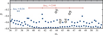
In figure 3 we provide a more detailed view of the spectrum for the subdomain
 $\mathsf{M}$
comprising the leading, least stable, global modes. The leading global modes consist of multiple local maxima of growth rate for varying frequency, centred around the maximum growth-rate peak at
 $\unicode[STIX]{x1D714}_{r}\approx 43.91$
and
 $\unicode[STIX]{x1D714}_{i}\approx -0.29$
. The frequency difference between consecutive maxima is nearly constant and equal to
 $\unicode[STIX]{x0394}\unicode[STIX]{x1D714}_{r}\approx 2.44$
, and the temporal growth rate for the local maxima is approximately
 $\unicode[STIX]{x1D714}_{i}\approx -0.29$
. Between the peaks, the frequency difference of neighbouring eigenvalues is
 $\unicode[STIX]{x0394}\unicode[STIX]{x1D714}_{r}\approx 0.34$
, and their minimum growth-rate is approximately
 $\unicode[STIX]{x1D714}_{i}\approx -0.60$
. These spectral features (also reported in Fosas de Pando et al.
Reference Fosas de Pando, Schmid and Sipp2014) have been found to be in good agreement with numerical simulations and experiments.
Zoomed view of the global spectrum showing the least stable (or leading) global modes. The modes
 $\mathsf{M}_{1}$
–
 $\mathsf{M}_{4}$
are considered in more detail, and the corresponding eigenvalues are
 $\unicode[STIX]{x1D714}_{\mathsf{M}_{1}}\approx 43.91-0.29\text{i}$
,
 $\unicode[STIX]{x1D714}_{\mathsf{M}_{2}}\approx 44.63-0.61\text{i}$
,
 $\unicode[STIX]{x1D714}_{\mathsf{M}_{3}}\approx 45.59-0.59\text{i}$
and
 $\unicode[STIX]{x1D714}_{\mathsf{M}_{4}}\approx 46.25-0.34\text{i}$
. The relative residuals for the displayed modes fall below
 $10^{-5}$
.

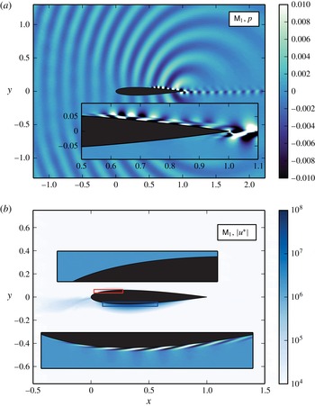
(a) Spatial structure of the global mode labelled
 $\mathsf{M}_{1}$
, visualised by the real part of the associated near-field pressure levels, and the real part of the streamwise velocity levels in the vicinity of the aerofoil surface (inset). The mode has been normalised by the maximum value of the velocity field in the near wake
 $1<x<1.2$
. (b) Spatial structure of the associated adjoint global mode (labelled
 $\mathsf{M}_{1}$
in figure 3), visualised by the magnitude of the streamwise velocity levels, and the real part in the insets.

Evolution of the streamwise velocity peak along the aerofoil chord (a) on the suction surface and (b) on the pressure surface of the aerofoil for the leading modes labelled
 $\mathsf{M}_{1}$
–
 $\mathsf{M}_{4}$
in figure 3. (c,d) Same for the adjoint streamwise velocity peak. (e,f) Same for the direct mode, adjoint mode and wavemaker corresponding to
 $\mathsf{M}_{1}$
.

The corresponding least stable mode, associated with
 $\mathsf{M}_{1}$
in figure 3, is shown in figure 4(a). It is visualised by the pressure and reveals a complex spatial structure that emphasises a distinct disturbance wavepacket downstream of both separation bubbles, a vortex street shedding into the wake and a pronounced acoustic wave radiating from the aerofoil’s trailing edge. The inset, showing the streamwise velocity component, displays the modal features near the trailing edge, where a wavepacket structure on the suction side links, via the trailing edge, to a more compact disturbance stemming from the pressure side. As we will demonstrate below, this link between the pressure-side and suction-side dynamics is a quintessential characteristic of the tonal-noise phenomenon. It is equally important to note that the acoustic wave reaches both the pressure- and suction-side boundary layer where it retriggers a respective boundary-layer instability; this feature has been illustrated in Fosas de Pando et al. (Reference Fosas de Pando, Schmid and Sipp2014) by following an impulse response. The global mode
 $\mathsf{M}_{1}$
thus represents in one structure the various components of the double feedback loop: boundary-layer instability
 $\rightarrow$
acoustic wave
 $\rightarrow$
reseeding mechanism.
The description of the perturbation dynamics only in terms of global modes is incomplete if no further thoughts are given to the processes by which an initial perturbation (or, equivalently, a given forcing) projects onto the various direct global modes. In more physical terms, such a projection is linked to receptivity mechanisms. As was argued earlier, the adjoint global modes represent a powerful theoretical concept to assess receptivity mechanisms of the flow: within the limitation of linear disturbance analysis, an arbitrary perturbation can be expressed as a linear combination of global modes
 $\boldsymbol{u}=\sum _{j}a_{j}\boldsymbol{v}_{j}$
. In order to obtain the coefficients
 $a_{i}$
, we take the inner product on both sides with the corresponding adjoint global mode
 $\boldsymbol{w}_{i}$
. By invoking the bi-orthogonality condition, and noting that we have chosen the adjoint global modes such that
 $\langle \boldsymbol{w}_{i},\boldsymbol{v}_{i}\rangle =1$
, we arrive at
 $a_{i}=\langle \boldsymbol{w}_{i},\boldsymbol{u}\rangle$
. From an optimisation point of view, the adjoint global mode corresponds to the perturbation that produces the largest projection onto the corresponding direct mode, and its norm
 $\Vert \boldsymbol{w}_{i}\Vert$
constitutes a useful measure to evaluate overall receptivity. More physically, the adjoint mode corresponding to
 $\mathsf{M}_{1}$
will pinpoint the location, structure and flow components where the double feedback loop (via the pressure and suction side) that sustains
 $\mathsf{M}_{1}$
is most easily excited or otherwise manipulated.
Figure 4(b) displays the adjoint mode that corresponds to the direct mode
 $\mathsf{M}_{1}$
, visualised by the adjoint streamwise velocity
 $u^{\ast }$
. Within the domain depicted in this figure, the adjoint mode is spatially localised in the boundary layer on the pressure side between approximately 20 % and 50 % of the chord (see inset). The amplitude of the adjoint mode, with the normalisation convention introduced above, confirms a significant amount of receptivity of the structure displayed in figure 4(a) to localised perturbations in the pressure-side boundary layer. The receptivity anywhere else, including the suction-side boundary layer, is orders of magnitude less. These results suggest that in order to break the feedback loop that maintains the least stable mode (and its associated acoustic foot print) a minimal effort is required if control is applied at the location where the corresponding adjoint is maximal, i.e. at 30 % of the chord on the pressure side.
A clearer picture of the least stable
 $\mathsf{M}$
-modes emerges when considering the direct and adjoint global modes corresponding to
 $\mathsf{M}_{1}$
–
 $\mathsf{M}_{4}$
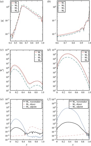
in figure 3. In figure 5(a,b), we depict the streamwise velocity peak along the aerofoil chord on the suction and pressure surfaces of the aerofoil, respectively, for the four modes
 $\mathsf{M}_{1}$
–
 $\mathsf{M}_{4}$
. All four modes display a similar behaviour: on the suction side, up to 60 % of the chord, we observe a significant rise, after which the peak streamwise velocity steadily decreases towards the trailing edge; on the pressure side, we have a continual rise in the peak velocity, which becomes even more pronounced as the trailing edge is approached. The corresponding adjoint modes are displayed in figure 5(c,d), visualised by the adjoint streamwise velocity magnitude
 $|u^{\ast }|$
in the suction- and pressure-side boundary layers, respectively. Recalling the normalisation convention of the adjoint modes, the magnitude of
 $u^{\ast }$
is a meaningful measure to compare the relative receptivity of different direct modes. As was the case for the direct modes, the spatial distribution of the four adjoint global modes for
 $\mathsf{M}_{1}$
–
 $\mathsf{M}_{4}$
is very similar: the support of the adjoint mode is highly localised on the pressure-surface boundary layer, between the leading edge and upstream of the separation point, i.e.
 $0.2<x<0.5$
, with the maximum value at approximately
 $10^{9}$
. Among the four modes considered,
 $\mathsf{M}_{1}$
and
 $\mathsf{M}_{4}$
show nearly the same receptivity, while
 $\mathsf{M}_{2}$
and
 $\mathsf{M}_{3}$
display an order of magnitude less. Some receptivity is also observed in the free-stream (not shown) in the region where the base flow convects perturbations to the pressure-surface boundary layer, i.e. near the stagnation line. We note that the levels of receptivity on the suction surface are nearly
 $10^{3}$
times smaller than the corresponding receptivity measures on the pressure surface.
The difference in spatial support between the direct global modes and their adjoint equivalents is striking and has implications for the understanding of the underlying physical phenomena. It is well-known that in convectively unstable shear flows, a common manifestation of the non-normality of the Navier–Stokes operator is the spatial separation between the direct and adjoint global modes in the downstream and upstream direction (Chomaz Reference Chomaz2005), respectively. The direct global modes typically display exponential growth in the convectively unstable region, and if the flow is stable downstream, their amplitudes reach nearly a constant value in that region. Conversely, from a global point of view, the adjoint modes show increased spatial support in the region where a localised perturbation yields a large projection onto the direct global mode. From a local point of view, the adjoint modes show the highest value where a localised pointwise perturbation undergoes maximum amplification by means of the instability mechanisms present in the flow.
In our case, however, the direct global mode is concentrated on the suction surface and in the near wake, whereas the adjoint global mode is predominantly located on the pressure surface. Paradoxically, the perturbation that causes the largest growth of a global mode with spatial support on the suction surface is not convectively linked to the location on the pressure surface that causes maximum receptivity. As a consequence, the spatial structure of the adjoint mode suggests a different route for the excitation of the instabilities in the flow via (i) the growth of instabilities by convective mechanisms on the pressure surface, (ii) the scattering of an acoustic wave at the trailing edge, and (iii) the receptivity at the leading edge, where the suction-surface boundary layer displays convective instabilities. This receptivity mechanism prevails over the direct growth of instabilities on the suction surface as the total spatial growth along the pressure surface is larger than the analogous growth on the suction surface. This observation is supported by previous experiments (Nash, Lowson & McAlpine Reference Nash, Lowson and McAlpine1999) and numerical calculations (Desquesnes et al. Reference Desquesnes, Terracol and Sagaut2007): the frequency of the dominant tone in the spectrum coincides with the most amplified frequency along the pressure surface based on local stability theory.
Besides, not all modes appear to be equally receptive. We depict the magnitude of the adjoint mode on the suction surface, figure 5(c), and on the pressure surface, figure 5(d). It can be observed that the receptivity on the pressure surface to streamwise velocity perturbations is higher for the modes at the peaks in growth rate,
 $\mathsf{M}_{1}$
and
 $\mathsf{M}_{4}$
, than for modes
 $\mathsf{M}_{2}$
and
 $\mathsf{M}_{3}$
. As discussed before, the frequencies of the modes
 $\mathsf{M}_{1}$
and
 $\mathsf{M}_{4}$
are in excellent agreement with the frequencies that appear in the acoustic spectrum of the nonlinear numerical simulation.
The occurrence of multiple peaks in the sound spectrum cannot solely be explained by the convective instability properties of the boundary layer: the range of frequencies where the boundary layer displays convective growth is larger than the frequency difference between the peaks. In this respect, it is suggested that global effects further discretise the components that are most amplified.
3.2.1 Wavemaker analysis and structural sensitivity
In figure 5(e,f) we display the peak amplitude of the wavemaker of the leading mode
 $\mathsf{M}_{1}$
(together with the respective contribution of the direct and adjoint modes) along the suction- and pressure-side boundary layer, respectively. We observe that the spatial support of the wavemaker is closer to the adjoint than to the direct mode, since the compactness of the adjoint is more pronounced than that of the direct mode.
This fact suggests that the individual leading eigenfrequency is more sensitive to operator perturbations
 $\unicode[STIX]{x1D63C}$
on the pressure surface of the aerofoil (and, in particular, upstream of the separation point) than in the rest of the domain. A first indication of the wavemaker location on the pressure surface has been reported in the previous numerical study of Desquesnes et al. (Reference Desquesnes, Terracol and Sagaut2007), where they state: ‘The computation of the amplification ratio for different chordwise stations and the same
 $x_{0}$
[distance from the leading edge] shows that the most amplified frequency is constant and equal to
 $845~\text{Hz}$
from
 $x/c=0.7$
to
 $x/c=0.96$
. The tone noise frequency is therefore selected before the boundary-layer separation.’ In this respect, the wavemaker describes the localised region in the flow that imposes its dynamics on the remaining flow. The results presented here are therefore in good agreement with both numerical and experimental studies; we can quote Paterson et al. (Reference Paterson, Vogt, Fink and Much1973) who report: ‘A boundary-layer trip wire was found to have no effect on the tone when placed at various chordwise positions on the suction surface of this airfoil but caused the tone to disappear when placed forward of 80 % chord on the pressure surface.’
The above observations, describing the sensitivity of the flow to changes in the base flow, are in excellent agreement with the spatial location of the wavemaker. However, it is less clear whether a link between the triggering of the pressure-surface boundary layer and the small operator perturbations (considered above) can be established and whether this link can be made responsible for the vanishing of tonal-noise effects.
Another implication is related to the choice of base flow. Although the instantaneous flow and the mean flow are not steady solutions of the Navier–Stokes equations, the time residual at the pressure-surface boundary layer upstream of the separation bubble is very small. This indicates that the modes of interest exhibit sufficient robustness, provided that the pressure-surface boundary layer remains unaltered.
3.3 High-frequency modes: suction-surface shear-layer instabilities
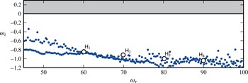
We next consider in figure 6 the range of high frequencies of the global spectrum (with respect to the leading eigenfrequencies). A rather continuous branch is observed, and for our analysis four representative global modes are selected and identified, to assess the parameterisation along the high-frequency branch.
Global spectrum displaying high frequencies
 $\unicode[STIX]{x1D714}>45$
; the modes labelled
 $\mathsf{H}_{1}$
–
 $\mathsf{H}_{4}$
will be analysed further. Their associated eigenfrequencies are:
 $\unicode[STIX]{x1D714}_{\mathsf{H}_{1}}=60.06-0.85\text{i}$
,
 $\unicode[STIX]{x1D714}_{\mathsf{H}_{2}}=69.90-0.92\text{i}$
,
 $\unicode[STIX]{x1D714}_{\mathsf{H}_{3}}=80.17-1.00\text{i}$
, and
 $\unicode[STIX]{x1D714}_{\mathsf{H}_{4}}=89.97-1.05\text{i}$
. The residual associated with the iterative eigenvalue solver is smaller than
 $5\times 10^{-3}$
.

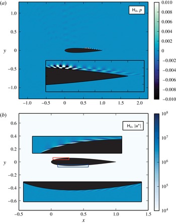
Direct and adjoint global mode corresponding to
 $\mathsf{H}_{4}$
indicated in figure 6, visualised by the real part of the pressure field (a) and absolute value of the adjoint streamwise velocity (b). The insets, showing the real part of the streamwise velocity, give more details of the respective flow fields.

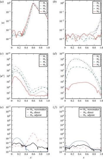
Evolution of the streamwise velocity peak along the aerofoil chord (a) on the suction surface and (b) on the pressure surface of the aerofoil for the high-frequency modes labelled
 $\mathsf{H}_{1}$
–
 $\mathsf{H}_{4}$
in figure 6. (c,d) Same for the adjoint streamwise velocity peak. (e,f) Same for the direct mode, adjoint mode and wavemaker corresponding to
 $\mathsf{H}_{4}$
.

The direct mode
 $\mathsf{H}_{4}$
, depicted in figure 7(a) in terms of the pressure, is singled out and shown to display features that are concentrated in the detached area of the suction-side boundary layer, together with its effect on the shear layer past the reattachment point. A wavepacket pattern with a distinct spatial wavenumber is observed, with its maximum near 60 % of the chord and a steadily diminishing amplitude as it sheds towards the trailing edge and into the aerofoil’s wake. An involvement of instability features from the pressure-side boundary layer is not observed. We thus conclude that high-frequency modes, such as
 $\mathsf{H}_{4}$
, describe the Kelvin-Helmholtz-like instabilities induced by the separated suction-side boundary layer.
Only a very small amount of acoustic radiation is present in this mode, far less than the acoustic footprint of any of the leading modes: the high-frequency vortex-shedding dynamics of the suction-side separation bubble is a very minor contributor to the tonal-noise sound pressure levels.
Again, the corresponding adjoint mode provides information about the receptivity of this instability and its origin. The adjoint
 $\mathsf{H}_{4}$
-mode is displayed in figure 7(b), visualised by the adjoint streamwise velocity. The insets clearly show non-zero adjoint amplitude at both the pressure and suction side of the aerofoil; the suction side amplitudes are, however, orders of magnitude larger, indicating a preferred receptivity location near the upper leading edge (10 % chord) of the aerofoil. On the pressure side, the region of maximum receptivity is at approximately 50 % of the chord.
A more complete analysis of the high-frequency modes and their structural connection to the leading modes of the previous section consists of a comparison of several (direct and adjoint) modes along the high-frequency branch in terms of their amplitudes and localisation along the pressure and suction side of the aerofoil. To this end, we investigate four selected high-frequency modes, labelled
 $\mathsf{H}_{1}$
–
 $\mathsf{H}_{4}$
in figure 6, and display their streamwise velocity amplitudes in the suction- and pressure-side boundary layer. On the suction side (see figure 8
a), the modal structure remains very similar as we move from
 $\mathsf{H}_{1}$
to
 $\mathsf{H}_{4}$
: a strong exponential rise in amplitude towards a peak near 60 % of the chord, followed by an exponential decay towards the trailing edge. On the pressure side (see figure 8
b), however, we observe markedly larger differences. While the high-frequency modes
 $\mathsf{H}_{1}$
and
 $\mathsf{H}_{2}$
(which are closest in frequency to the leading modes) are characterised by a steady and pronounced rise in amplitude towards the trailing edge, this rise is absent in the higher-frequency modes
 $\mathsf{H}_{3}$
and
 $\mathsf{H}_{4}$
. In effect, towards the lower edge of the high-frequency branch, the direct modes still resemble the leading modes in shape, i.e. a dominant localised structure on the suction side, coupled to an even more localised counterpart near the pressure side’s trailing edge. As we progress towards higher frequencies, only the suction-side structures remains; the pressure-side amplitudes are considerably smaller along the entire chord. This observation is in accordance with the structure of
 $\mathsf{H}_{4}$
(figure 7
a), where only features near the suction-side separation bubble and its wake have been detected.
The analysis of the adjoint modes confirms the above findings. On the suction side (see figure 8
c), we observe an amplitude evolution for
 $\mathsf{H}_{1}$
reminiscent of the leading modes (compare to figure 5
c). As higher frequencies are approached, however, the maximum amplitudes decay by two orders of magnitude, while preserving the approximate dependence on the chordwise coordinate direction. More importantly, this decay in amplitude for higher-frequency modes is more pronounced on the pressure side (see figure 8
d), where
 $\mathsf{H}_{1}$
still displays a receptivity of
 $10^{9},$
comparable to the value for the leading modes, while
 $\mathsf{H}_{4}$
shows a receptivity measure more than four orders of magnitude smaller. In other words, higher-frequency modes increasingly become unreceptive to perturbations on the pressure side of the aerofoil. It should be stressed again that the choice of normalisation allows direct comparison of the direct and adjoint modal structures.
The wavemaker analysis of the highest-frequency mode
 $\mathsf{H}_{4}$
is depicted in figure 8(e,f) for the suction and pressure side, respectively. Few distinguishing features can be found in these amplitude curves, indicating the absence of a strong selection principle for localisation of the receptivity measure in the case of high-frequency modes.
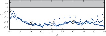
Low-frequency modes in the spectrum. The modes labelled
 $\mathsf{L}_{1}$
–
 $\mathsf{L}_{4}$
are depicted in figure 10, and the corresponding eigenvalues are
 $\unicode[STIX]{x1D714}_{\mathsf{L}_{1}}=29.98-0.63\text{i}$
,
 $\unicode[STIX]{x1D714}_{\mathsf{L}_{2}}=20.15-0.70\text{i}$
,
 $\unicode[STIX]{x1D714}_{\mathsf{L}_{3}}=10.12-0.65\text{i}$
and
 $\unicode[STIX]{x1D714}_{\mathsf{L}_{4}}=0.001-0.19\text{i}$
.

3.4 Low-frequency modes: separation-bubble flapping and reattached flow dynamics
The global modes at lower frequencies (compared to the leading modes) capture the dynamics of the unsteady separation bubbles together with the induced flow dynamics in the reattachment zone. The low-frequency part of the spectrum, displayed in figure 9, shows a continuous branch reaching up to the quasi-steady (
 $\unicode[STIX]{x1D714}_{r}\approx 0$
) regime. Along this branch, we select four representative modes, labelled
 $\mathsf{L}_{1}$
through
 $\mathsf{L}_{4}$
, which we will analyse in more detail to determine the qualitative changes in the modal structures and their receptivity as we approach the lower-frequency limit.
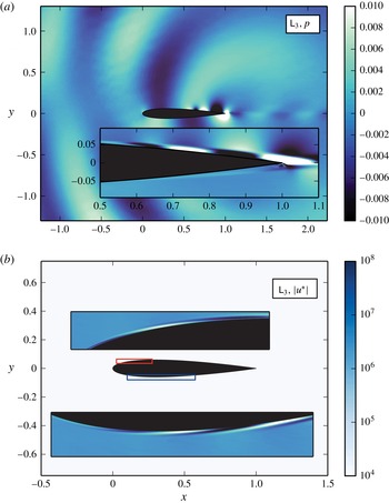
The shape of mode
 $\mathsf{L}_{3}$
, visualised by pressure, is displayed in figure 10(a). It shows flow features concentrated on the separated region of the suction-side boundary layer. Due to the low frequency, large-scale spatial structures are encountered. They describe the ‘breathing’ unsteadiness of the separation bubble, coupled to the remainder of the complex flow dynamics which even includes a weak but non-negligible acoustic component. The inset shows more details, such as the link via the trailing edge to the separated flow region on the pressure surface: a vortical element near the very end of the pressure surface – an essential part of the pressure-surface dynamics – is clearly visible.
The corresponding adjoint mode (figure 10
b) shows non-zero features on both the pressure and the suction side of the aerofoil. Either structure is characterised by low-wavenumber elements due to the low temporal frequency. While the suction-side structure is concentrated near 20 % of the chord, the pressure-side structure is localised near the half-chord. In terms of amplitude, the two adjoint structures are nearly equal (approximately
 $10^{4}$
using our standard normalisation), suggesting that triggering this particular mode
 $\mathsf{L}_{3}$
is equally effective by perturbations in either of the two general locations identified by the adjoint mode.
Direct and adjoint global modes corresponding to
 $\mathsf{L}_{3}$
indicated in figure 9, showing streamwise velocity (a) and adjoint streamwise velocity (b). The insets give more details of the respective flow fields.

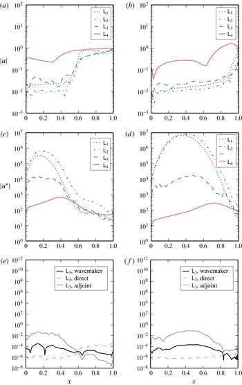
Evolution of the streamwise velocity peak along the aerofoil chord (a) on the suction surface and (b) on the pressure surface of the aerofoil for the low-frequency modes labelled
 $\mathsf{L}_{1}$
–
 $\mathsf{L}_{4}$
in figure 9. (c,d) Same for the adjoint streamwise velocity peak. (e,f) Same for the direct mode, adjoint mode and wavemaker corresponding to
 $\mathsf{L}_{3}$
.

As before, more insight can be gained by evaluating the direct and adjoint streamwise velocity along the pressure and suction side for each of the four selected modes
 $\mathsf{L}_{1,\ldots ,4}$
. Figure 11(a,b) presents the results for the direct modes, where panel (a) shows localisation of the modal structure on the suction surface in the second half of the aerofoil, nearly independent of the frequency, except for the quasi-steady case
 $\mathsf{L}_{4}$
. On the pressure surface (panel b), similar tendencies are observed: modes
 $\mathsf{L}_{1,\ldots ,3}$
exhibit nearly identical behaviour, reflecting the presence of a strong separation bubble near the trailing edge. Again, the quasi-steady mode
 $\mathsf{L}_{4}$
shows a markedly different shape.
Figure 11(c,d) displays the adjoint modes
 $\mathsf{L}_{1,\ldots ,4}$
evaluated along the suction and pressure surface of the aerofoil, respectively. The suction surface depicts a dominant receptivity measure (quantified by the adjoint streamwise velocity) near the upstream half of the aerofoil, which is rather pronounced for
 $\mathsf{L}_{1}$
, closest in frequency to the leading modes, and gradually diminishes in amplitude (without too strong a change in shape) as the frequency is lowered. In this respect, the curve for adjoint mode
 $\mathsf{L}_{1}$
should be compared to the one for adjoint mode
 $\mathsf{M}_{1}$
(from figure 5
c): similarities are clearly present. The same can be said about the analogous results for the pressure surface (figure 11
d). For
 $\mathsf{L}_{1}$
we nearly recover the receptivity curves of the leading modes (see 5
d), although at lower maximum amplitude. Moreover, the low-frequency modes
 $\mathsf{L}_{1,2}$
inherit from the leading modes their preference of the pressure surface (over the suction surface) regarding the most effective manner of triggering the associated global direct modes. This preference is more conspicuous for the leading modes (with more than two orders of magnitude in receptivity measure
 $\max _{x}|u^{\ast }|$
between the two surfaces); nonetheless, it is also present (with one order of magnitude between the two surfaces) for the low-frequency modes
 $\mathsf{L}_{1,2}$
. As the frequency is further lowered, such as for mode
 $\mathsf{L}_{3}$
, the partiality in receptivity of the pressure surface vanishes, and mode
 $\mathsf{L}_{3}$
is as easily triggered (and manipulated) from the pressure as from the suction surface. This result can be inferred from figure 11(c,d).
Finally, the wavemaker analysis (see figure 11
e,f) for the low-frequency mode
 $\mathsf{L}_{2}$
shows that both surfaces of the aerofoil are nearly equally structurally stable. In addition, similar to the high-frequency modes, there is little that distinguishes specific regions on either airfoil surface as far as structural stability is concerned.
4 Summary and conclusions
A complete and global analysis of the compressible flow about a NACA-0012 aerofoil at a
 $2^{\circ }$
angle of attack, a chord-based Reynolds number of
 $2\times 10^{5}$
and a Mach number of 0.4 has been presented, with emphasis on extracting the dominant physical mechanisms underlying the generation of tonal noise. This flow configuration was chosen to match typical mean flow characteristics described in the experimental work of Paterson et al. (Reference Paterson, Vogt, Fink and Much1973), Nash et al. (Reference Nash, Lowson and McAlpine1999) and the numerical simulations of Desquesnes et al. (Reference Desquesnes, Terracol and Sagaut2007). The modal structures span a rather wide frequency range, but only a few modes (in the leading
 $\mathsf{M}$
-category) contain a significant acoustic component to account for the observed sound pressure levels as well as the observed frequencies. An analysis of the adjoint modal structures gives insight into receptivity and sensitivity measures for the associated direct counterparts, and a pointwise superposition of direct and adjoint modes identifies the wavemaker region of maximal structural instability. It should be stressed that the details of noise generation near the trailing edge – the subject of a large body of literature – are of less importance in our study, since they only represent one component of a global feedback loop; rather, it is the details of the complete feedback loop, and the role of its components, that we are interested in.
In the case of the acoustically active
 $\mathsf{M}$
-modes this type of analysis revealed that tonal noise is most easily triggered, or manipulated, at the pressure side of the aerofoil, more specifically near 35 % of the chord. This finding corroborates previous observations, including the early investigations of Paterson et al. (Reference Paterson, Vogt, Fink and Much1973) as well as the numerical simulations of Desquesnes et al. (Reference Desquesnes, Terracol and Sagaut2007) and Fosas de Pando et al. (Reference Fosas de Pando, Schmid and Sipp2014). It identifies the most sensitive part of the hydrodynamic-acoustic feedback loop and suggests the placement of actuators or surface elements on the aerofoil’s upstream pressure side for an active or passive strategy to weaken or suppress acoustic tones.
With the direct
 $\mathsf{M}$
-modes appearing predominantly on the suction side of the aerofoil and the associated adjoint modes showing compact support on the pressure side, it is worth pointing out that these two structures are not convectively connected. This is in contrast to previous studies where the upstream sensitivity and the downstream amplification are solely joined by an advective process via the base or mean flow. In our present case, a link between the input and output structures for the
 $\mathsf{M}$
-modes is established by the acoustic waves, which form an integral part of the feedback loop. Ascribing the generation of tonal noise solely to boundary layer instabilities would amount to an incomplete description of the overall mechanism.
For completeness, modes with lower and higher frequency (compared to the
 $\mathsf{M}$
-branch) have also been included in our analysis. Either type shows rather negligible acoustic radiation, and, according to their adjoint counterparts, they can be most easily manipulated from the suction side (in case of high-frequency modes) or equally from the suction and pressure side (for the low-frequency modes). As the frequency range of the leading
 $\mathsf{M}$
-modes is approached, however, the aerofoil’s pressure side increasingly dominates the receptivity of either modes.
Lastly, the present analysis of the tonal noise problem using adjoint techniques showcases a tool which provides valuable insight into instability mechanisms that entail a complex interplay of multiple physical processes. The same analysis would, for example, also be appropriate for thermoacoustic or combustion systems where hydrodynamic, acoustic and reactive instabilities co-exist and interact in a non-trivial manner. Similar to the present study, a global stability and receptivity analysis would capture pertinent feedback loops and suggest means of disrupting them most efficiently.