3.1. Kinematics model

Tab In the O–XYZ coordinate system, under ideal conditions, when constructing the closed-loop vector equation, the position vector r _A of point A can be expressed as:

(1) \begin{align} \left\{\begin{array}{l} {\boldsymbol{r}}_{A}={\boldsymbol{b}}_{i}+l_{di}\cdot {\boldsymbol{e}}_{di}-{\boldsymbol{a}}_{i}\\ {\boldsymbol{r}}_{A}=l_{c}\cdot {\boldsymbol{e}}_{c} \end{array}\right. \left(i=1,2,3\right) \end{align}

Among them, l _di and e _di respectively represent the rod length and unit vector of the i-th UPS driving branch chain, and l _c and e _c respectively represent the rod length and unit vector of the UP-constraint branch chain.

b _i is the position vector of point B _i in the coordinate system O–XYZ, and a _i is the position vector of the center point A _i of the Hooke hinge in the composite spherical hinge in the coordinate system O–XYZ. R _A is the rotation matrix of the coordinate system A-x^′y^′z^′ relative to the coordinate system O–XYZ, and a _iM is the position vector of point A _i under the coordinate system A-x^′y^′z^′ of the moving platform M.

The rod length and unit vector of the UPS driving branch chain can be expressed as:

(2) \begin{align} \left\{\begin{array}{l} l_{di}=\sqrt{\left(l_{c}\cdot {\boldsymbol{e}}_{c}+{\boldsymbol{a}}_{i}-{\boldsymbol{b}}_{i}\right)^{\mathrm{T}}\cdot \left(l_{c}\cdot {\boldsymbol{e}}_{c}+{\boldsymbol{a}}_{i}-{\boldsymbol{b}}_{i}\right) }\\ {\boldsymbol{e}}_{di}=\frac{l_{c}\cdot {\boldsymbol{e}}_{c}+{\boldsymbol{a}}_{i}-{\boldsymbol{b}}_{i}}{l_{di}} \end{array}\right. \left(i=1,2,3\right) \end{align}

The rod length and unit vector of the UP constraint branched chain can be expressed as:

(3) \begin{align} l_{c}=\sqrt{{{\boldsymbol{r}}_{A}}^{\mathrm{T}}\cdot {\boldsymbol{r}}_{A} } \, ; \, {\boldsymbol{e}}_{c}=\frac{{\boldsymbol{r}}_{A}}{l_{c}} \end{align}

In order to express the position of the end point P of the lapping and polishing disk in the coordinate system O-XYZ, the pose relationship between each coordinate system of the serial mechanism is established.

Under the coordinate system P ₂-x _p2 y _p2 z _p2, the position vector P _m2 of the endpoint P of the lapping and polishing disk can be expressed as:

(4) \begin{align} {\boldsymbol{P}}_{m2}=\left[\cos \left(\omega _{m}t\right)\cdot d_{0}\sin \left(\omega _{m}t\right)\cdot d_{0} -d_{0z}\right]^{\mathrm{T}} \end{align}

R _p2 is the rotation matrix of the coordinate system P ₂-x _p2 y _p2 z _p2 relative to the coordinate system P ₁-x _p1 y _p1 z _p1, and P ₂ is the position vector of the coordinate origin P ₂ in the coordinate system P ₁-x _p1 y _p1 z _p1.

Under the coordinate system P ₁-x _p1 y _p1 z _p1, the position vector P _m1 of the end point P of the lapping and polishing disk can be expressed as:

(5) \begin{align} {\boldsymbol{P}}_{m1}={\boldsymbol{P}}_{2}+{\boldsymbol{R}}_{p2}\cdot {\boldsymbol{P}}_{m2} \, ; \, {\boldsymbol{P}}_{2}=\left[\cos \left(\theta _{p}\right)\cdot d_{2}0 -\sin \left(\theta _{p}\right)\cdot d_{2}\right]^{\mathrm{T}} \end{align}

R _P1 is the rotation matrix of the coordinate system P ₁-x _p1 y _p1 z _p1 with respect to the coordinate system A-x^′y^′z^′ , and P ₁ is the position vector of the coordinate origin P ₁ in the coordinate system A-x^′y^′z^′ .

Under the coordinate system A-x^′y^′z^′ , the position vector P _mA of the end point P of the lapping and polishing disk can be expressed as:

(6) \begin{align} {\boldsymbol{P}}_{mA}={\boldsymbol{P}}_{1}+{\boldsymbol{R}}_{P1}\cdot {\boldsymbol{P}}_{m1} \, ; \, {\boldsymbol{P}}_{1}=\left[\begin{array}{lll} 0 & 0 & -d_{1} \end{array}\right]^{\mathrm{T}} \end{align}

To sum up, the position vector P of the end point P of the lapping and polishing disk in the coordinate system O-XYZ can be expressed as:

(7) \begin{align} {\boldsymbol{P}}={\boldsymbol{r}}_{A}+{\boldsymbol{R}}_{A}\cdot {\boldsymbol{P}}_{mA}={\boldsymbol{r}}_{A}+{\boldsymbol{R}}_{A}\cdot \left({\boldsymbol{P}}_{1}+{\boldsymbol{R}}_{P1}\cdot \left({\boldsymbol{P}}_{2}+{\boldsymbol{R}}_{P2}\cdot {\boldsymbol{P}}_{m2}\right)\right) \end{align}

3.2. Geometric error model

3.2.1. Establishment of a local coordinate system

For the ideal compound spherical hinge of the 5-DOF (Degree of Freedom) hybrid mirror caption mutually perpendicular. However, due to the limitations of processing and assembly conditions, it is difficult for the compound spherical hinge to meet these ideal requirements. Therefore, angular and linear errors exist between the rotation axes of the compound spherical hinge and those of the Hooke’s joint.

According to the right-hand rule, considering the geometric error conditions, the local coordinate system of the error model is established. In the fixed coordinate system O-XYZ, point O is the intersection of the common perpendicular line between the near-frame axis and the far-frame axis of the Hooke hinge in the UP-branch chain and the near-frame axis. The X-axis passes through points B _i (i = 1,2,3) and point O, and the Y-axis coincides with the near-frame axis of the Hooke hinge in the UP-branch chain. In the UPS-branched Hooke hinge connection system B _i -x _i y _i z _i , the point B _i (i = 1,2,3) is the intersection of the common perpendicular line between the near-frame axis and the far-frame axis of the Hooke hinge in branch chain i with the near-frame axis. The x _i (i = 1,2,3) axis coincides with the near-frame axis of the Hooke hinge in branch chain i, and the z _i axis is perpendicular to the far-frame axis. In the UPS-branched chain i connection system N _i -u _i v _i w _i , the point N _i (i = 1,2,3) is the intersection of the axis of branch chain i and the far-frame axis of the Hooke hinge. The v _i axis coincides with the far-frame axis, and the w _i axis aligns with the axis of branch chain i, pointing from point N _i in the direction of the compound spherical hinge. In the connection system of the outer ring of the compound spherical hinge bearing S _i -x _si y _si z _si , point S _i is the intersection point of the perpendicular line drawn from the center point O _fi of the outer ring of the bearing in the direction of the hinge connection shaft A _i B _i . The z _si axis is aligned with the axis of the UPS branch chain, and the x _si axis is perpendicular to the surface of the outer ring of the bearing. Similarly, in the connection system of the inner ring of the compound spherical hinge bearing T _i -x _Ti y _Ti z _Ti , point T _i is the intersection point of the perpendicular line drawn from the center point O _ei of the inner ring of the bearing in the direction of the hinge connection shaft A _i B _i . The z _Ti axis points along the hinge connection shaft toward the moving platform, and the x _Ti axis is perpendicular to the surface of the inner ring of the bearing. In the compound spherical hinge connection shaft system M _i -u _i ^′v _i ^′w _i ^′ , point M _i is the intersection point of the axis of the hinge connection shaft and the axis of the Hooke hinge far frame. The v _i ^′ axis coincides with the far frame axis, and the w _i ^′ axis aligns with the axis direction of the hinge connection shaft, pointing towards point T _i . In the Hooke hinge connection system A _i -x _i ^′y _i ^′z _i ^′ of the compound spherical hinge, point A _i is the intersection point of the common perpendicular line between the near frame axis and the far frame axis of the Hooke hinge on the moving platform and the near frame axis. The x _i ^′ axis coincides with the near frame axis, and the z _i ^′ axis is perpendicular to the far frame axis. In the moving platform connection system A-x^′y^′z^′ , point A is the intersection point of the axis of the UP branched chain and the plane defined by points A _i (i = 1,2,3), the y^′ axis is in the same direction as the Y axis in the system O-XYZ, and the z^′ axis points towards the fixed platform along the direction of the UP branched chain. In the Hooke hinge connection system O-X ₀ Y ₀ Z ₀ of the UP branched chain, the Y ₀ axis coincides with the near frame axis of the Hooke hinge in the UP branched chain, the Z ₀ axis is perpendicular to the far frame axis, and the X ₀ axis is determined according to the right-hand rule. The local coordinate system of its closed-branched chain is shown in Figure 2.

Figure 2.

The local coordinate system of the closed-branched chain.

3.2.2. Geometric error model

Under ideal conditions, the position vector equation of the closed chain O - B _i - N _i - S _i - T _i - M _i - A _i - A - o in the parallel mechanism can be expressed as:

(8) \begin{align} {\boldsymbol{r}}_{A}+{\boldsymbol{R}}_{A}\cdot {\boldsymbol{a}}_{i}+\delta _{i}\cdot {\boldsymbol{e}}_{i}={\boldsymbol{b}}_{i}+\gamma _{i}\cdot {\boldsymbol{e}}_{j} \left(i,j=1,2,3\right) \end{align}

Among them, e _i and δ _i are, respectively, the direction vector and the length of the rod connecting the i-th UPS branched chain to the moving platform in the coordinate system O-XYZ, and e _j and γ _j are, respectively, the direction vector and the length of the rod connecting the j-th UPS branched chain to the fixed platform in the coordinate system O-XYZ.

By combining the Eq. (7), we can obtain Eq. (9).

(9) \begin{align} \left\{\begin{array}{l} {\boldsymbol{P}}+{\boldsymbol{R}}_{A}\cdot {\boldsymbol{a}}_{i}+\delta _{i}\cdot {\boldsymbol{e}}_{i}={\boldsymbol{b}}_{i}+\gamma _{i}\cdot {\boldsymbol{e}}_{j}+{\boldsymbol{R}}_{A}\cdot {\boldsymbol{P}}_{mA}\\[4pt] {\boldsymbol{e}}_{i}={\boldsymbol{R}}_{A}\cdot {\boldsymbol{R}}_{Ai}\cdot {\boldsymbol{R}}_{Mi}\cdot {\boldsymbol{R}}_{Ti}\cdot {\boldsymbol{e}}\mathit{'}\\[4pt] {\boldsymbol{e}}_{j}={\boldsymbol{R}}_{Bj}\cdot {\boldsymbol{R}}_{Nj}\cdot {\boldsymbol{R}}_{Sj}\cdot {\boldsymbol{e}}\mathit{'} \end{array}\right. \end{align}

Based on the definition of the coordinate system, under the first-order perturbation condition, the relevant geometric error sources are introduced; therefore, the position vector can be expressed as:

(10) \begin{align} \left\{\begin{array}{l} {\boldsymbol{P}}+{\unicode{x0394}} {\boldsymbol{P}}+\left[\begin{array}{l} E+\boldsymbol{\theta }_{A\times } \end{array}\right]\cdot {\boldsymbol{R}}_{A}\cdot \left({\boldsymbol{a}}_{i}+{\unicode{x0394}} {\boldsymbol{a}}_{i}\right)+D_{1}={\boldsymbol{b}}_{i}+{\unicode{x0394}} {\boldsymbol{b}}_{i}+D_{2}+D_{3}\\[4pt] D_{1}=\left[\begin{array}{l} E+\boldsymbol{\theta }_{A\times } \end{array}\right]\cdot {\boldsymbol{R}}_{A}\cdot \left[{\boldsymbol{E}}+\boldsymbol{\theta }_{Ai\times }\right]\cdot {\boldsymbol{R}}_{Ai}\cdot \left[{\boldsymbol{E}}+\boldsymbol{\theta }_{Mi\times }\right]\\[4pt] \quad\quad\cdot {\boldsymbol{R}}_{Mi}\cdot \left({\unicode{x0394}} {\boldsymbol{m}}_{i}+\left[{\boldsymbol{E}}+\boldsymbol{\theta }_{Ti\times }\right]\cdot {\boldsymbol{R}}_{Ti}\cdot \left(\left(\delta _{i}+{\unicode{x0394}} \delta _{i}\right)\cdot {\boldsymbol{e}}'+{\unicode{x0394}} {\boldsymbol{S}}_{i}\right)\right)\\[4pt] D_{2}=\left[{\boldsymbol{E}}+\boldsymbol{\theta }_{Bi\times }\right]\cdot {\boldsymbol{R}}_{Bi}\cdot \left[{\boldsymbol{E}}+\boldsymbol{\theta }_{Ni\times }\right]\cdot {\boldsymbol{R}}_{Ni}\cdot \left({\unicode{x0394}} {\boldsymbol{n}}_{i}+\left[{\boldsymbol{E}}+\boldsymbol{\theta }_{Si\times }\right]\cdot {\boldsymbol{R}}_{Si}\cdot \left(\left(\gamma _{i}+{\unicode{x0394}} \gamma _{i}\right)\cdot {\boldsymbol{e}}'\right)\right)\\[4pt] D_{3}=\left[\begin{array}{l} E+\boldsymbol{\theta }_{A\times } \end{array}\right]\cdot {\boldsymbol{R}}_{A}\cdot \left({\boldsymbol{P}}_{1}+{\unicode{x0394}} {\boldsymbol{P}}_{1}+\left[{\boldsymbol{E}}+\boldsymbol{\theta }_{P1\times }\right]{\boldsymbol{R}}_{P1}\cdot \left({\boldsymbol{P}}_{2}+{\unicode{x0394}} {\boldsymbol{P}}_{2}+\left[{\boldsymbol{E}}+\boldsymbol{\theta }_{P2\times }\right]{\boldsymbol{R}}_{P2}\cdot \left({\boldsymbol{P}}_{m2}+{\unicode{x0394}} {\boldsymbol{P}}_{m2}\right)\right)\right) \end{array}\right. \end{align}

Among them, Δ P represents the position error of point P in the coordinate system O-XYZ; $\boldsymbol{\theta}$ _A represents the attitude error of the coordinate system A-x^′y^′z^′ in the coordinate system O-XYZ, and $\boldsymbol{\theta}$ _A× denotes the skew-symmetric matrix of $\boldsymbol{\theta}$ _A , with other skew-symmetric matrices expressed similarly; Δ a _i represents the position error of A _i in the coordinate system A-x^′y^′z^′ ; Δ b _i represents the position error of B _i in the coordinate system O-XYZ; Δ m _i represents the position error of M _i in the coordinate system A _i -x _i ^′y _i ^′z _i ^′ ; Δ S _i represents the position error of S _i in the coordinate system T _i -x _Ti y _Ti z _Ti ; Δ n _i represents the position error of N _i in the coordinate system B _i -x _i y _i z _i ; Δ $\boldsymbol{\delta}$ _i represents the offset of the actual position relative to the theoretical position of the connection part of the i-th UPS branched chain and the moving platform in the coordinate system M _i -u _i ^′v _i ^′w _i ^′ ; Δ $\boldsymbol{\gamma}$ _i represents the offset of the actual position relative to the theoretical position of the connection part of the i-th UPS branched chain and the fixed platform in the coordinate system N _i -u _i v _i w _i ; Δ P ₁ represents the position error of P ₁ in the coordinate system A-x^′y^′z^′ ; Δ P ₂ represents the position error of P ₂ in the coordinate system P ₁-x _p1 y _p1 z _p1; Δ P _m2 represents the error of the end point P of the lapping and polishing disk in the coordinate system P ₂-x _p2 y _p2 z _p2.

Firstly, the closed-chain vector equation under the first-order perturbation condition is linearized. Then, the difference between this equation and the closed-chain vector equation under the ideal condition is taken. Finally, the dot product of both sides of the resulting equation with e _j ^T is performed,

(11) \begin{align} \left\{\begin{array}{l} {\boldsymbol{e}}_{j}^{\mathrm{T}}\cdot {\unicode{x0394}} {\boldsymbol{P}}+E_{1}+E_{2}={\boldsymbol{e}}_{j}^{{\boldsymbol{T}}}\cdot {\unicode{x0394}} {\boldsymbol{b}}_{i}+\cos \psi _{i}\cdot {\unicode{x0394}} z_{ni}+{\unicode{x0394}} \gamma _{i}+E_{3}+E_{4}+E_{5}\\[3pt] E_{1}={\boldsymbol{e}}_{j}^{\mathrm{T}}\cdot {\boldsymbol{R}}_{A}\cdot {\unicode{x0394}} {\boldsymbol{a}}_{iM}+\left({\boldsymbol{a}}_{i}\times {\boldsymbol{e}}_{i}\right)^{\mathrm{T}}\cdot \boldsymbol{\theta }_{A}+{\boldsymbol{e}}_{j}^{\mathrm{T}}\cdot {\boldsymbol{R}}_{A}\cdot \left({\boldsymbol{R}}_{Ai}\cdot {\boldsymbol{R}}_{Mi}\cdot {\unicode{x0394}} {\boldsymbol{m}}_{i}+{\boldsymbol{R}}_{Ai}\cdot {\boldsymbol{R}}_{Mi}\cdot {\boldsymbol{R}}_{Ti}\cdot {\unicode{x0394}} {\boldsymbol{S}}_{i}\right)+{\boldsymbol{e}}_{j}^{\mathrm{T}}\cdot {\unicode{x0394}} \delta _{i}\cdot {\boldsymbol{e}}_{i}\\[3pt] E_{2}=\left(\left(\delta _{i}\cdot {\boldsymbol{e}}_{i}\right)\times {\boldsymbol{e}}_{j}\right)^{\mathrm{T}}\cdot \boldsymbol{\theta }_{A}+\left(\left(\delta _{i}\cdot {\boldsymbol{e}}_{i}\right)\times \left({\boldsymbol{R}}_{A}^{\mathrm{T}}\cdot {\boldsymbol{e}}_{j}\right)\right)^{\mathrm{T}}\cdot \boldsymbol{\theta }_{Ai}+\left(\left({\boldsymbol{R}}_{Ti}\cdot \delta _{i}\cdot {\boldsymbol{e}}'\right)\times \left({\boldsymbol{R}}_{Mi}^{\mathrm{T}}\cdot {\boldsymbol{R}}_{Ai}^{\mathrm{T}}\cdot {\boldsymbol{R}}_{A}^{\mathrm{T}}\cdot {\boldsymbol{e}}_{i}\right)\right)^{\mathrm{T}}\cdot \boldsymbol{\theta }_{Mi}\\[3pt] E_{3}={\boldsymbol{e}}_{j}^{\mathrm{T}}\cdot {\boldsymbol{R}}_{A}\cdot \left({\unicode{x0394}} {\boldsymbol{P}}_{1}+{\boldsymbol{R}}_{P1}\cdot {\unicode{x0394}} {\boldsymbol{P}}_{2}+{\boldsymbol{R}}_{P1}\cdot {\boldsymbol{R}}_{P2}\cdot {\unicode{x0394}} {\boldsymbol{P}}_{m2}\right)+\left(\left({\boldsymbol{R}}_{P2}\cdot {\boldsymbol{P}}_{m2}\right)\times \left({\boldsymbol{R}}_{P1}^{\mathrm{T}}\cdot {\boldsymbol{R}}_{A}^{\mathrm{T}}\right)\cdot {\boldsymbol{e}}_{j}\right)^{\mathrm{T}}\cdot \boldsymbol{\theta }_{P2}\\[3pt] E_{4}=\left(\left({\boldsymbol{R}}_{P1}\cdot {\boldsymbol{P}}_{2}\right)\times {\boldsymbol{e}}_{j}\right)^{\mathrm{T}}\cdot \boldsymbol{\theta }_{P1}+\left(\left({\boldsymbol{R}}_{P1}\cdot {\boldsymbol{R}}_{P2}\cdot {\boldsymbol{P}}_{m2}\right)\times {\boldsymbol{e}}_{j}\right)^{\mathrm{T}}\cdot \boldsymbol{\theta }_{P1}\\[3pt] E_{5}=\left(\left({\boldsymbol{R}}_{A}\cdot {\boldsymbol{P}}_{1}\right)\times {\boldsymbol{e}}_{j}\right)^{\mathrm{T}}\cdot \boldsymbol{\theta }_{A}+\left(\left({\boldsymbol{R}}_{A}\cdot {\boldsymbol{R}}_{P1}\cdot {\boldsymbol{P}}_{2}\right)\times {\boldsymbol{e}}_{j}\right)^{\mathrm{T}}\cdot \boldsymbol{\theta }_{A}+\left(\left({\boldsymbol{R}}_{A}\cdot {\boldsymbol{R}}_{P1}\cdot {\boldsymbol{R}}_{P2}\cdot {\boldsymbol{P}}_{m2}\right)\times {\boldsymbol{e}}_{j}\right)^{\mathrm{T}}\cdot \boldsymbol{\theta }_{A} \end{array}\right. \end{align}

and after simplification, the Eq. (11) can be obtained.

The direction vector e _Bi of the connection part of the UPS branch chain and the fixed platform B _i S _i in the coordinate system B _i -x _i y _i z _i can be expressed as:

(12) \begin{align} \begin{array}{l} {\boldsymbol{e}}_{Bi}=R\left(x_{i},\theta _{i}\right)\cdot R\left(y_{i},\psi _{i}\right)\cdot {\boldsymbol{e}}'={\boldsymbol{R}}_{Ni}\cdot {\boldsymbol{R}}_{Si}\cdot {\boldsymbol{e}}' \end{array} \end{align}

In the system O-XYZ, e _di can be expressed as e _di = R _Bi $ \cdot{\boldsymbol{e}}$ _Bi , where R _Bi is the rotation matrix of the coordinate system B _i -x _i y _i z _i relative to the coordinate system O-XYZ. Therefore, it can be expressed as:

(13) \begin{align} {\boldsymbol{e}}_{Bi}={\boldsymbol{R}}_{Bi}^{-1}\cdot {\boldsymbol{e}}_{di} \end{align}

By combining the Eqs. (12) and (13), we can obtain Eq. (14).

(14) \begin{align} {\boldsymbol{R}}_{Bi}^{-1}\cdot {\boldsymbol{e}}_{di}=\left[\begin{array}{lll} \sin \psi _{i} & -\sin \theta _{i}\cos \psi _{i} & \cos \theta _{i}\cos \psi _{i} \end{array}\right]^{\mathrm{T}} \end{align}

Among them, e _di can be obtained through the inverse kinematics solution, R _Bi can be expressed according to the geometric relationship between the coordinate systems as:

(15) \begin{align} {\boldsymbol{R}}_{B1}=R\left(Z,180^{\circ }\right);\,{\boldsymbol{R}}_{B2}=R\left(Z,60^{\circ }\right);\,{\boldsymbol{R}}_{B3}=R\left(Z,300^{\circ }\right) \end{align}

Through inverse solution, the expressions of $\psi$ _i and θ _i can be expressed as:

(16) \begin{align} \left\{\begin{array}{l} \psi _{i}= \ arcsin \left({\boldsymbol{R}}_{Bi}^{-1}\cdot {\boldsymbol{e}}_{di}\left(1\right)\right)\\[4pt] \theta _{i}=-arctan \left({\boldsymbol{R}}_{Bi}^{-1}\cdot {\boldsymbol{e}}_{di}\left(2\right)/{\boldsymbol{R}}_{Bi}^{-1}\cdot {\boldsymbol{e}}_{di}\left(3\right)\right) \end{array}\right. \left(i=1,2,3\right) \end{align}

Similarly, the direction vector e _Ai of the part T _i A _i where the UPS branch is connected to the moving platform in the coordinate system A _i -x _i ^′y _i ^′z _i ^′ can be expressed as:

(17) \begin{align} \begin{array}{l} {\boldsymbol{e}}_{Ai}=R\left(x_{i}^{\mathrm{'}},\tau _{i}\right)\cdot R\left(y_{i}^{\mathrm{'}},\varphi _{i}\right)\cdot {\boldsymbol{e}}'={\boldsymbol{R}}_{Mi}\cdot {\boldsymbol{R}}_{Ti}\cdot {\boldsymbol{e}}' \end{array} \end{align}

In the coordinate system O-XYZ, e _di can be expressed as e _di = −R _A $ \cdot{\boldsymbol{R}}$ _Ai $ \cdot{\boldsymbol{e}}$ _Ai , where R _Ai is the rotation matrix of the coordinate system A _i -x _i ^′y _i ^′z _i ^′ relative to the coordinate system A-x^′y^′z^′ . Through calculation, it can be expressed as:

(18) \begin{align} {\boldsymbol{e}}_{Ai}=-{\boldsymbol{R}}_{Ai}^{-1}\cdot {\boldsymbol{R}}_{A}^{-1}\cdot {\boldsymbol{e}}_{di} \end{align}

By combining the Eqs. (17) and (18), we can obtain Eq. (19).

(19) \begin{align} {\boldsymbol{R}}_{Ai}^{-1}\cdot {\boldsymbol{R}}_{A}^{-1}\cdot {\boldsymbol{e}}_{di}=\left[\begin{array}{ccc} -\sin \varphi _{i} & \sin \tau _{i}\cos \varphi _{i} & -\cos \tau _{i}\cos \varphi _{i} \end{array}\right]^{\mathrm{T}} \end{align}

Among them, e _di can be obtained through the inverse kinematics solution, and R _Ai can be expressed according to the geometric relationship between the coordinate systems as:

(20) \begin{align} {\boldsymbol{R}}_{A1}=R\left(z',0^{\circ }\right);\quad {\boldsymbol{R}}_{A2}=R\left(z',120^{\circ }\right);\quad {\boldsymbol{R}}_{A3}=R\left(z',240^{\circ }\right) \end{align}

Through inverse solution, the expressions of $ \phi$ _i and τ _i can be expressed as:

(21) \begin{align} \left\{\begin{array}{l} \varphi _{i}=-\mathit{arcsin }\left({\boldsymbol{R}}_{Ai}^{-1}\cdot {\boldsymbol{R}}_{A}^{-1}\cdot {\boldsymbol{e}}_{di}\left(1\right)\right)\\[4pt] \tau _{i}=-\mathit{arctan }\left({\boldsymbol{R}}_{Ai}^{-1}\cdot {\boldsymbol{R}}_{A}^{-1}\cdot {\boldsymbol{e}}_{di}\left(2\right)/{\boldsymbol{R}}_{0j}^{-1}\cdot {\boldsymbol{R}}_{A}^{-1}\cdot {\boldsymbol{e}}_{di}\left(3\right)\right) \end{array}\right.\left(i=1,2,3\right) \end{align}

Under ideal conditions, the position vector r _A of the center point A of the moving platform is given by r _A = l _c $ \cdot{\boldsymbol{e}}$ _c . Combining this with the position vector equation of the end point P of the lapping and polishing disk, we can be expressedas:

(22) \begin{align} {\boldsymbol{P}}={\boldsymbol{R}}_{O}\cdot {\boldsymbol{o}}+l_{c}\cdot {\boldsymbol{e}}_{c}+{\boldsymbol{R}}_{A}\cdot {\boldsymbol{P}}_{mA} \end{align}

Based on the definition of the coordinate system, under the first-order perturbation condition, the relevant geometric error sources are introduced; consequently, the position vector can be expressed as:

(23) \begin{align} {\unicode{x0394}} {\boldsymbol{P}}={\boldsymbol{R}}_{O}\cdot {\unicode{x0394}} {\boldsymbol{o}}+{\unicode{x0394}} l_{c}\cdot {\boldsymbol{e}}_{c}+l_{c}\cdot {\unicode{x0394}} {\boldsymbol{e}}_{c}+D_{3} \end{align}

Among them, Δ e _c = $\boldsymbol{\theta}$ _A × e _c , o and Δ o represent the position vector and position error of point o in the coordinate system O-X ₀ Y ₀ Z ₀ ; R _O is the rotation matrix of the coordinate system O-X ₀ Y ₀ Z ₀ relative to the coordinate system O-XYZ, and Δl _c represents the offset of the actual position of the UP-branch chain relative to the theoretical position in the coordinate system O-XYZ. Then, the position vector equation of the UP-branch chain can be expressed as:

(24) \begin{align} {\unicode{x0394}} {\boldsymbol{P}}={\boldsymbol{R}}_{O}\cdot {\unicode{x0394}} {\boldsymbol{o}}+{\unicode{x0394}} l_{c}\cdot {\boldsymbol{e}}_{c}+l_{c}\cdot \boldsymbol{\theta }_{A}\times {\boldsymbol{e}}_{c}+D_{3} \end{align}

Under the condition of considering only linear errors, the attitude vector equation for the UP branch can be expressed as:

(25) \begin{align} \boldsymbol{\theta }_{A}=\boldsymbol{\theta }_{\mathrm{P}}+{\boldsymbol{R}}_{O}\cdot \boldsymbol{\theta }_{0}+{\unicode{x0394}} \phi _{0}\cdot {\boldsymbol{e}}_{0} \end{align}

Among them, $\boldsymbol{\theta}$ _P represents the attitude error of the coordinate system O-X ₀ Y ₀ Z ₀ relative to the coordinate system O-XYZ; $\boldsymbol{\theta}$ ₀ represents the attitude error of the coordinate system o-xyz relative to the coordinate system O-X ₀ Y ₀ Z ₀ ; and Δ $ \phi$ ₀ represents the relative torsional error of the guide rails on both sides of the UP branched chain in the coordinate system O-XYZ.

During the working process, this less-degree-of-freedom parallel mechanism will generate coupled motion in the restricted directions, which is accompanied by the generation of end pose errors. The geometric error sources that cause this type of pose error are termed uncompensated error sources.

In order to facilitate the subsequent kinematic calibration research, it is necessary to separate the compensable and non-compensable error sources. For this purpose, the vectors in the closed vector equation are projected onto the driving direction and the constraint direction of the corresponding branch chain, respectively. That is, multiply both sides of the position vector equation of the UP-branch chain by e _y ^T and e _x ^T, respectively, and the following can be expressed as:

(26) \begin{align} \left\{\begin{array}{l} {\boldsymbol{e}}_{y}^{\mathrm{T}}\cdot {\unicode{x0394}} P+l_{c}\cdot {\boldsymbol{e}}_{x}^{\mathrm{T}}\cdot \boldsymbol{\theta }_{A}={\boldsymbol{e}}_{y}^{\mathrm{T}}\cdot {\boldsymbol{R}}_{O}\cdot {\unicode{x0394}} o+{\boldsymbol{e}}_{y}^{\mathrm{T}}\cdot D_{3}\\[4pt] {\boldsymbol{e}}_{x}^{\mathrm{T}}\cdot {\unicode{x0394}} P-l_{c}\cdot {\boldsymbol{e}}_{y}^{\mathrm{T}}\cdot \boldsymbol{\theta }_{A}={\boldsymbol{e}}_{x}^{\mathrm{T}}\cdot {\boldsymbol{R}}_{O}\cdot {\unicode{x0394}} o+{\boldsymbol{e}}_{x}^{T}\cdot D_{3} \end{array}\right. \end{align}

The direction vector S of the common perpendicular line between the two rotational axes in the UP-branched Hooke’s joint can be expressed as:

(27) \begin{align} {\boldsymbol{S}}={\boldsymbol{R}}\left(Y,\theta _{0}\right)\cdot {\boldsymbol{e}}'=\left[\begin{array}{lll} \sin \theta _{0} & 0 & \cos \theta _{0} \end{array}\right]^{\mathrm{T}} \end{align}

Multiplying both sides of the UP branched chain attitude vector equation by S ^T, respectively, we can be expressed as:

(28) \begin{align} {\boldsymbol{S}}^{\mathrm{T}}\cdot \boldsymbol{\theta }_{A}=\sin \theta _{0}\cdot \theta _{xp}+\cos \theta _{0}\cdot \theta _{zp}+\theta _{z0}+{\unicode{x0394}} \phi _{0}\cdot \cos \psi _{0} \end{align}

By organizing Eqs. (11), (26), and (28), the end pose error matrix of the lapping and polishing disk can be obtained as follows:

(29) \begin{align} \left[\begin{array}{l} {\unicode{x0394}} {\boldsymbol{P}}\\ {\unicode{x0394}} \boldsymbol{\theta } \end{array}\right]=\left[\begin{array}{l} {\boldsymbol{J}}_{a}\\ {\boldsymbol{J}}_{c} \end{array}\right]^{-1}\cdot \left[\begin{array}{l@{\quad}l} {\boldsymbol{A}} & 0\\ 0 & {\boldsymbol{B}} \end{array}\right]\cdot \left[\begin{array}{l} \boldsymbol{\varepsilon }_{a}\\ \boldsymbol{\varepsilon }_{c} \end{array}\right]={\boldsymbol{J}}\cdot \left[\begin{array}{l} \boldsymbol{\varepsilon }_{a}\\ \boldsymbol{\varepsilon }_{c} \end{array}\right] \end{align}

Among them, the independent compensable error source: $\boldsymbol{\varepsilon }_{a}=[\begin{array}{lll} \boldsymbol{\varepsilon }_{a1} & \boldsymbol{\varepsilon }_{a2} & \boldsymbol{\varepsilon }_{a3} \end{array}]^{\mathrm{T}}$ .

Non-independent and non-compensable error source: $\boldsymbol{\varepsilon }_{c}=[\begin{array}{lllll} {\unicode{x0394}} {\boldsymbol{O}}_{0} & \theta _{xp} & \theta _{zp} & \theta _{z0} & {\unicode{x0394}} \phi _{0} \end{array}]^{\mathrm{T}}$ .

(30) \begin{align} \left\{\begin{array}{l} \begin{array}{l} \boldsymbol{\varepsilon }_{ai}=\left[\begin{array}{l@{\quad}l@{\quad}l@{\quad}l@{\quad}l@{\quad}l@{\quad}l@{\quad}l@{\quad}l} {\unicode{x0394}} {\boldsymbol{b}}_{i} & {\unicode{x0394}} Z_{ni} & {\unicode{x0394}} l_{i} & {\unicode{x0394}} {\boldsymbol{a}}_{i} & {\unicode{x0394}} {\boldsymbol{m}}_{i} & {\unicode{x0394}} \delta _{i} & {\unicode{x0394}} {\boldsymbol{S}}_{i} & \theta _{Ai} & \theta _{Mi} \end{array}\right]^{\mathrm{T}} \\ \\ {\boldsymbol{A}}=\left[\begin{array}{c@{\quad}c@{\quad}c} a_{11} & 0 & 0\\ 0 & a_{22} & 0\\ 0 & 0 & a_{33} \end{array}\right] ;\, {\boldsymbol{B}}=\left[\begin{array}{c@{\quad}c@{\quad}c@{\quad}c@{\quad}c} {\boldsymbol{e}}_{y}^{\mathrm{T}}\cdot {\boldsymbol{R}}_{O} & 0 & 0 & 0 & 0\\ {\boldsymbol{e}}_{x}^{\mathrm{T}}\cdot {\boldsymbol{R}}_{O} & 0 & 0 & 0 & 0\\ 0 & \sin \theta _{0} & \cos \theta _{0} & 1 & \cos \psi _{0} \end{array}\right] \end{array}\\ \\ {\boldsymbol{J}}_{a}=\left[\begin{array}{l@{\quad}l} {\boldsymbol{e}}_{1}^{\mathrm{T}} & \left({\boldsymbol{a}}_{1}\times {\boldsymbol{e}}_{1}\right)^{\mathrm{T}}+\left(\left({\boldsymbol{R}}_{A}\cdot \delta _{1}\cdot {\boldsymbol{e}}_{11}\right)\times {\boldsymbol{e}}_{1}\right)^{\mathrm{T}}\\[3pt] {\boldsymbol{e}}_{2}^{\mathrm{T}} & \left({\boldsymbol{a}}_{2}\times {\boldsymbol{e}}_{2}\right)^{\mathrm{T}}+\left(\left({\boldsymbol{R}}_{A}\cdot \delta _{2}\cdot {\boldsymbol{e}}_{22}\right)\times {\boldsymbol{e}}_{2}\right)^{\mathrm{T}}\\[3pt] {\boldsymbol{e}}_{3}^{\mathrm{T}} & \left({\boldsymbol{a}}_{3}\times {\boldsymbol{e}}_{3}\right)^{\mathrm{T}}+\left(\left({\boldsymbol{R}}_{A}\cdot \delta _{3}\cdot {\boldsymbol{e}}_{33}\right)\times {\boldsymbol{e}}_{3}\right)^{\mathrm{T}} \end{array}\right];\, {\boldsymbol{J}}_{c}=\left[\begin{array}{c@{\quad}c} {\boldsymbol{e}}_{y}^{\mathrm{T}} & l_{0}\cdot {\boldsymbol{e}}_{x}^{\mathrm{T}}\\[3pt] {\boldsymbol{e}}_{x}^{\mathrm{T}} & -l_{0}\cdot {\boldsymbol{e}}_{y}^{\mathrm{T}}\\[3pt] 0 & {\boldsymbol{S}}^{\mathrm{T}} \end{array}\right] \end{array}\right. \end{align}

The error source $\varepsilon$ _a that affects the pose accuracy comprises 63 items, among which 15 items have a theoretical value of 0. The error source $\varepsilon$ _c consists of 7 items, with 1 item having a theoretical value of 0. $\varepsilon$ _a includes the position and angle errors of the Hooke hinges distributed on the fixed platform, the pose error between the near-frame axis and the far-frame axis in the hinges, the length error of the ball screw component, the position and angle errors of the compound spherical hinges distributed on the moving platform, the pose error between the Hooke hinge axes in the compound hinges, the length error of the connection shaft between the Hooke hinge and the angular contact bearing, and the axial error of the angular contact bearing. $\varepsilon$ _c includes the position and angle errors of the Hooke hinges distributed in the UP branched chain, the pose error between the near-frame axis and the far-frame axis in the hinges, and the torsional error of the guide rail in the UP branched chain.

4.1. Identification model

The core content of kinematic parameter calibration is to establish the residual equation between the measured pose error and the theoretical pose error at the end of the lapping and polishing disk and then identify and solve the geometric error parameters with the goal of minimizing the end-effector pose error. Figure 3 shows the calibration experiment body.

Figure 3.

Calibration experiment body.

$\varepsilon$ _a and $\varepsilon$ _c jointly affect the pose. The coupling between these two error sources will lead to a rank reduction in the identification matrix, making Δ $\varepsilon$ unidentifiable. Therefore, $\varepsilon$ _a is used to reconstruct the error model for identification. Under the observed configurations k (k = 1 to n), the residual equation between the measurement error of the end poses and the theoretical error is expressed as:

(31) \begin{align} {\boldsymbol{e}}_{k}=\left({\boldsymbol{P}}_{m,k}-{\boldsymbol{P}}_{e,k}\right)-\left({\boldsymbol{P}}_{t,k}-{\boldsymbol{P}}_{e,k}\right)=\delta {\boldsymbol{P}}_{m,k}-{\boldsymbol{H}}\cdot {\unicode{x0394}} \boldsymbol{\varepsilon }_{k} \end{align}

Among them, P _m,k and P _t,k are, respectively, the measured value and theoretical value of the end pose of the lapping and polishing disk, considering the influence of the error source; P _e,k is the expected value of the end pose of the lapping and polishing disk without considering the influence of the error source; δ P _m,k is the measurement error of the end pose of the lapping and polishing disk; H is the error transfer matrix, composed of the first 63 columns of the full error transfer matrix J ; and Δ $\varepsilon$ _k = $\varepsilon$ _a represents the geometric error parameter to be identified.

To obtain the optimal solution of the identification model, specifically the least squares solution, an error functional is constructed to minimize the sum of squared residuals, leading to the following results.

(32) \begin{align} {\unicode{x0394}} \boldsymbol{\varepsilon }_{{\boldsymbol{k}}}=\left({\boldsymbol{H}}^{\mathrm{T}}\cdot {\boldsymbol{H}}\right)^{-1}\cdot {\boldsymbol{H}}^{\mathrm{T}}\cdot \boldsymbol{\delta }{\boldsymbol{P}}_{{\boldsymbol{m}},{\boldsymbol{k}}} \end{align}

4.2. Pose measurement and parameter identification

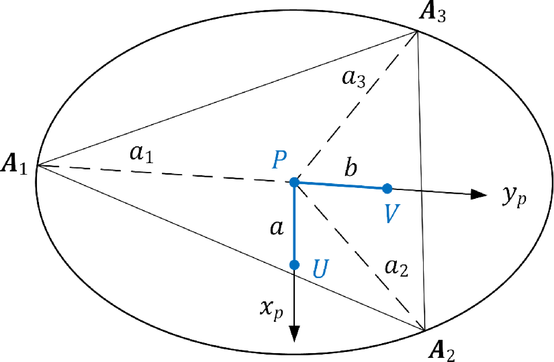
Based on the measurement values of each target point obtained from different observation points, the end pose of the lapping and polishing disk is calculated. Specifically, in the lapping and polishing disk coordinate system P-x _P y _P z _P , three targeted measurement points P, U, and V are set at the center point P and on the x _P and y _P coordinate axes, respectively. The positional relationship of the measurement points on the lapping and polishing disk is shown in Figure 4.

Figure 4.

Measuring points position.

The position vectors of the measurement points U and V under the coupled system P-x _P y _P z _P of the lapping and polishing disk can be expressed as:

(33) \begin{align} {\boldsymbol{U}}_{P}=\left[\begin{array}{lll} a & 0 & 0 \end{array}\right]^{\mathrm{T}} \, ; \, {\boldsymbol{V}}_{P}=\left[\begin{array}{lll} 0 & b & 0 \end{array}\right]^{\mathrm{T}} \end{align}

Among them, a is the distance between the measurement point P and U, and b is the distance between the measurement point P and V. When the lapping and polishing disk is in the observation configuration k, the position measurement values of the three-measurement points P, U, and V in the coordinate system O-XYZ are expressed as:

(34) \begin{align} \left\{\begin{array}{l} {\boldsymbol{P}}_{O,k}={\boldsymbol{P}}_{m,k}-{\boldsymbol{O}}_{m,k}=\left[\begin{array}{lll} x_{O,k}^{P} & y_{O,k}^{P} & z_{O,k}^{P} \end{array}\right]^{\mathrm{T}}\\[4pt] {\boldsymbol{U}}_{O,k}={\boldsymbol{U}}_{m,k}-{\boldsymbol{O}}_{m,k}=\left[\begin{array}{lll} x_{O,k}^{U} & y_{O,k}^{U} & z_{O,k}^{U} \end{array}\right]^{\mathrm{T}}\\[4pt] {\boldsymbol{V}}_{O,k}={\boldsymbol{V}}_{m,k}-{\boldsymbol{O}}_{m,k}=\left[\begin{array}{lll} x_{O,k}^{V} & y_{O,k}^{V} & z_{O,k}^{V} \end{array}\right]^{\mathrm{T}} \end{array}\right. \end{align}

It can be seen from the transformation relationship of the position vectors of each measurement point in different coordinate systems.

(35) \begin{align} \left\{\begin{array}{l} {\boldsymbol{R}}_{P}\cdot {\boldsymbol{U}}_{P}={\boldsymbol{U}}_{O,k}-{\boldsymbol{P}}_{O,k}=\left[x_{k}^{U} y_{k}^{U} z_{k}^{U}\right]^{\mathrm{T}}\\ {\boldsymbol{R}}_{P}\cdot {\boldsymbol{V}}_{P}={\boldsymbol{V}}_{O,k}-{\boldsymbol{P}}_{O,k}=\left[x_{k}^{V} y_{k}^{V} z_{k}^{V}\right]^{\mathrm{T}}\\ {\boldsymbol{R}}_{P}\cdot \left({\boldsymbol{U}}_{P}\times {\boldsymbol{V}}_{P}\right)=\left({\boldsymbol{U}}_{O,k}-{\boldsymbol{P}}_{O,k}\right)\times \left({\boldsymbol{V}}_{O,k}-{\boldsymbol{P}}_{O,k}\right) \end{array}\right. \end{align}

Among them, O _m,k is the position measurement value of the coordinate system O-XYZ in the measurement coordinate system O _m -x _m y _m z _m . R _P is the rotation matrix of the coordinate system P-x _P y _P z _P relative to the coordinate system O-XYZ.

Under the coordinate system O-XYZ, the measurement values of the end pose of the polishing disk are expressed as:

(36) \begin{align} {\boldsymbol{P}}_{O,k}=\left[x_{m,k}^{P}\, ; \, y_{m,k}^{P} \, ; \, z_{m,k}^{P} \, ; \, \arctan \frac{\left(z_{k}^{U}\cdot x_{k}^{V}-x_{k}^{U}\cdot z_{k}^{V}\right)}{\left(x_{k}^{U}\cdot y_{k}^{V}-y_{k}^{U}\cdot x_{k}^{V}\right)};\arcsin \frac{\left(z_{k}^{U}\cdot y_{k}^{V}-y_{k}^{U}\cdot z_{k}^{V}\right)}{ab};\arctan \frac{a\cdot x_{k}^{V}}{b\cdot x_{k}^{U}}\right] \end{align}

During the measurement process, the number and position distribution of observation points will have a certain impact on the identification accuracy. To ensure that the matrix ( H ^T $ \cdot{\boldsymbol{H}}$ is of full rank and the independent error source Δ $\varepsilon$ _k is identifiable, the number of observation configurations n should satisfy n > p/6, where p denotes the total number of independent error sources to be identified. Since there are 48 independent error sources to be identified, at least 8 observation configurations need to be selected.

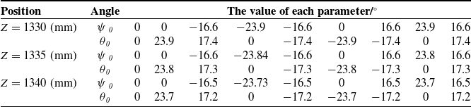
Since the workspace of the prototype is approximately cylindrical, the observation points are selected mainly within the range of the end’s primary movement. To ensure that the observation configurations can traverse all controllable degrees of freedom and make the measurement results reasonable and random to a certain extent, the observation points are uniformly distributed on both the circular ring of the working plane and at the center position. Considering that each independent error source primarily influences the end pose error in the edge area of the workspace, configurations with larger deflection angles around both the X-axis and Y-axis are selected for observation within this plane, thereby effectively improving the signal-to-noise ratio of measurement results.

Table I.

Pose parameters of observation points.

Therefore, three parallel and equidistant circular surfaces were selected along the Z-axis in the workspace of the mechanism. Nine points were uniformly selected on each circular surface, and a total of 27 poses were used for parameter identification. The pose parameters of the measurement points are shown in Table I.

Before parameter identification, it is necessary to verify the reliability of the identification model. Firstly, the accuracy rate ζ _i of parameter identification is defined, which is expressed in Eq. (37).

In the formula, ε _ai and ε _ai ^′ denote the prescribed value and the identified value of the geometric parameter associated with the i-th error source, respectively.

(37) \begin{align} \zeta _{i}=\frac{\left| \varepsilon _{ai}-\varepsilon _{ai}^{\mathrm{'}}\right| }{\left| \varepsilon _{ai}\right| } \end{align}

Secondly, 16 independent error sources in the branched chain were selected and defined. Based on the error model, the end pose error was analyzed. Finally, the parameter identification of the end pose error was conducted using the identification model, and the results are shown in Tables II and III.

It can be known that the error rate of geometric parameter identification ranges from 0 to 13.21%. Only one erroneous parameter achieves a relatively accurate identification result. However, a high identification error rate will significantly impact the position accuracy of the robot. The main reason for the poor identification accuracy is that during the parameter identification process, which involves tracing the error source, the inverse operation of the matrix ( H ^T $ \cdot{\boldsymbol{H}}$ is required, and inverting an ill-conditioned matrix often results in low solution accuracy. To analyze and evaluate the solution stability of this identification model, the condition number of the coefficient matrix is utilized as a metric for assessing the degree of ill-conditioning in the linear equation system. Specifically, a larger condition number of the matrix ( H ^T $ \cdot{\boldsymbol{H}}$ indicates a higher degree of ill-conditioning. When the condition number of the matrix ( H ^T $ \cdot{\boldsymbol{H}}$ exceeds 10³, the identification results become highly sensitive to measurement noise, which may cause significant deviations from the true values. For an arbitrary observed configuration, the calculated condition number is cond ( H ^T ⋅H ) = 2.855 × 10³⁶ >> 10³. This demonstrates that the robustness of the identification matrix is inadequate. Consequently, even a minor disturbance in ( H ^T $ \cdot{\boldsymbol{H}}$ can lead to reduced solution accuracy and degraded identification performance.

Table II.

Identification results of geometric parameters.

Table III.

Identification results of geometric parameters.

To address this ill-conditioned problem, an improved pivot element weighted iterative algorithm is employed for optimization. The core of this algorithm lies in preprocessing the coefficient matrix by adding a weight to its principal components, thereby reducing the condition number of the coefficient matrix. As the condition number decreases, the degree of ill-conditioning is mitigated. To further enhance the accuracy and stability of the solution, the algorithm is refined. Specifically, an intermediate variable is introduced, and through the error transfer method, the error of the solution vector is transferred to the intermediate variable. Subsequently, the intermediate variable is solved using the principal component weighted iterative method, achieving higher solution accuracy.

The identification model is formulated as the following system of equations.

(38) \begin{align} {\boldsymbol{Ax}} ={\boldsymbol{b}} \end{align}

Among them, $ {\boldsymbol{A}} ={\boldsymbol{H}}^{\mathrm{T}}{\boldsymbol{H}} ;\quad {\boldsymbol{x}}={\unicode{x0394}} \boldsymbol{\varepsilon }_{m} ;\quad {\boldsymbol{b}}={\boldsymbol{H}}^{\mathrm{T}}\delta {\boldsymbol{P}}_{m} $ .

By introducing intermediate variables and setting ${\boldsymbol{x}} ={\boldsymbol{c}}{\boldsymbol{y}}$ and ${\boldsymbol{c}} ={\boldsymbol{A}}^{\mathrm{T}}$ , where ${\boldsymbol{c}}$ is a non-singular matrix, the system of equations can be expressed as:

(39) \begin{align} \left({\boldsymbol{A}}{\boldsymbol{A}}^{\mathrm{T}}\right){\boldsymbol{y}}={\boldsymbol{b}} \end{align}

Based on the principal component weighting method, the system of equations can be expressed as:

(40) \begin{align} \left({\boldsymbol{A}}{\boldsymbol{A}}^{\mathrm{T}}+\alpha {\boldsymbol{E}}\right){\boldsymbol{y}}={\boldsymbol{b}}+\alpha {\boldsymbol{y}} \end{align}

Through successive iterations, the iterative equation can be expressed as:

(41) \begin{align} \left({\boldsymbol{A}}{\boldsymbol{A}}^{\mathrm{T}}+\alpha {\boldsymbol{E}}\right){\boldsymbol{y}}^{\left(\lambda +1\right)}={\boldsymbol{b}}+\alpha {\boldsymbol{y}}^{\lambda } \end{align}

Among them, $\lambda$ denotes the number of iterations. Setting ${\boldsymbol{y}}^{(\lambda +1)}={\boldsymbol{y}}^{\lambda }+{\boldsymbol{e}}^{\lambda }$ and combining the aforementioned formula, we can be expressed as:

(42) \begin{align} \left({\boldsymbol{A}}{\boldsymbol{A}}^{\mathrm{T}}+\alpha {\boldsymbol{E}}\right){\boldsymbol{e}}^{\left(\lambda \right)}={\boldsymbol{b}}-{\boldsymbol{A}}{\boldsymbol{A}}^{\mathrm{T}}{\boldsymbol{y}}^{\left(\lambda \right)} \end{align}

When ${\boldsymbol{e}}^{(\lambda )}$ is small enough, that is, when $\frac{\left\| {\boldsymbol{e}}^{\left(\lambda \right)}\right\| }{\left\| {\boldsymbol{y}}^{\left(\lambda \right)}\right\| }\leq \mu$ , the optimal solution of the equation system can be obtained.

The selection of the weighting factor $\alpha$ in the identification model plays a critical role during the iterative process. If $\alpha$ is too small, the change in the condition number will be limited, and the equation set will remain ill-conditioned. Conversely, if $\alpha$ is too large, it may result in an undesirably slow convergence rate. To achieve faster convergence while maintaining identification accuracy, it is essential to analyze how the condition number cond ( ${\boldsymbol{A}}{\boldsymbol{A}}^{\mathrm{T}}+\alpha {\boldsymbol{E}}$ ) of the identification matrix varies with the weighting factor $\alpha$ . The corresponding relationship is illustrated in Figure 5.

Figure 5.

The variation law of the condition number with changes in the weighting factor.

In this study, $\alpha$ is set to 240, resulting in cond ( ${\boldsymbol{A}}{\boldsymbol{A}}^{\mathrm{T}}+\alpha {\boldsymbol{E}}$ ) = 1.669. It can be observed that the condition number of the coefficient matrix in the identification model has been substantially reduced compared to its value prior to optimization.

Upon determining the value of the weighting factor, the identification algorithm is optimized using the improved principal component weighting iterative method, thereby enabling the solution of the geometric parameters to be identified. The iterative procedure is illustrated in Figure 6.

Figure 6.

Flowchart of improved pivot element weighted iterative algorithm.

Similarly, the 16 independent error sources of the branched chain were selected to perform parameter identification using an improved pivot element weighted iterative algorithm model. The identification values and set values were recorded as shown in Figure 7.

Figure 7.

The identification value and set value.

Based on the parameter identification results, the error rates of the 16 error sources of the branched chain identified directly by the least squares method and by the improved pivot element weighted iterative algorithm were respectively calculated, and the results are shown in Figure 8.

Figure 8.

Error rate of geometric parameter identification.

Figure 9.

Error values before and after calibration of the end position.

As shown in Figure 8, the error rate of the improved pivot element weighted iterative algorithm ranges from 0 to 5.122%. Among these, five parameters exhibit a relatively high identification accuracy. Compared with the identification results directly obtained by the least squares method, the error rate of the improved algorithm is significantly reduced, and the amplitude of error fluctuation is obviously decreased. This result indicates that this method can effectively enhance the accuracy of parameter identification results.

4.3. Kinematics calibration and simulation results

In the kinematic calibration process, geometric error sources are identified using the measured end pose errors, and the geometric parameters in the robot controller are modified based on these identification results to improve the robot’s motion accuracy.

On the basis of parameter identification using the improved pivot element weighted iterative algorithm, the end position error is compensated. For this purpose, 27 sets of observation configurations are established on three observation planes, and kinematic calibration is performed. To make the calibrated pose error more intuitive, only the position values in the three translational degrees of freedom are considered, and the results are shown in Figure 9. It can be seen from the result that using the improved pivot element weighted iterative algorithm for calibration significantly reduces the end pose error compared to the error before calibration.

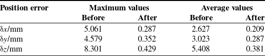
To further validate the reliability of kinematic calibration, Table IV presents the maximum and average values of the end position error before and after calibration. Additionally, the modulus of the position error, also known as the volumetric position error, is utilized to quantify the accuracy of the end pose.

It can be known that the maximum position error has decreased from (5.061, 4.579, 8.301) mm to (0.287, 0.352, 0.429) mm, and the maximum volumetric position error has decreased from 10.747 mm to 0.625 mm. The average position error has decreased from (2.627, 3.023, 5.408) mm to (0.209, 0.287, 0.381) mm, and the average volumetric position error has decreased from 6.729 mm to 0.521 mm. According to the data analysis, based on the improved pivot element weighted iterative algorithm, after kinematic calibration, both the maximum and average values of the end position error have decreased, and the accuracy of the mechanism has significantly improved.