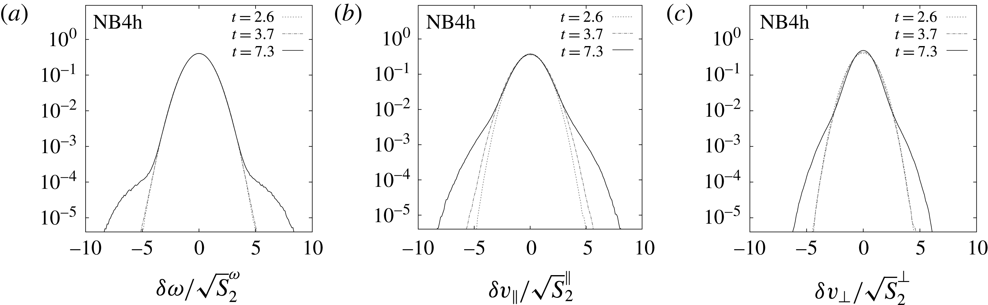
1 Introduction
Coherent vortices are an important flow component in both freely decaying and forced two-dimensional turbulence. In freely decaying turbulence, they form from localized extrema in the initial vorticity distribution and persist while weaker vorticity fluctuations in the background are strained into filaments, cascading enstrophy to dissipation scales. The vortices that survive this filamentation process merge, generating a self-similar population of vortex areas with a number density distribution that evolves algebraically in time (Benzi, Patarnello & Santangelo Reference Benzi, Patarnello and Santangelo1988; Carnevale et al. Reference Carnevale, McWilliams, Pomeau, Weiss and Young1991; Benzi et al. Reference Benzi, Collela, Briscolini and Santangelo1992; Weiss & McWilliams Reference Weiss and McWilliams1993; Dritschel et al. Reference Dritschel, Scott, Macaskill, Gottwald and Tran2008). At late times the coherent vortices contain almost all the flow energy.
When the inverse energy cascade is forced at intermediate scales coherent vortices again form, this time from localized vorticity extrema arising from random fluctuations in the forcing. In this case, the partition between coherent and background vorticity differs from that found in freely decaying two-dimensional (2-D) turbulence. Forcing continuously replenishes vorticity in the filamentary flow to compensate the loss of vorticity through the direct enstrophy cascade; background vorticity levels thus do not decay but equilibrate at a finite level. However, this level is much lower than that found within the coherent vortices, which again develop into localized regions in which vorticity is protected from strain and dissipation. Consequently a partition between strong, nearly circular coherent vortices and weak filamentary background flow may again be unambiguously defined (Smith & Yakhot Reference Smith and Yakhot1993; Borue Reference Borue1994; Scott Reference Scott2007; Vallgren Reference Vallgren2011; Fontane, Dritschel & Scott Reference Fontane, Dritschel and Scott2013; Burgess, Scott & Shepherd Reference Burgess, Scott and Shepherd2015; Burgess & Scott Reference Burgess and Scott2017); vortices are found to develop at the scales of the forcing and increase in area with time.
Burgess & Scott (Reference Burgess and Scott2017) recently proposed a scaling theory for the forced inverse energy cascade that predicts the number density distribution of vortices as a function of vortex area, where a vortex is defined as a region of intense vorticity bounded by a vorticity isoline, or level set of vorticity. By considering fundamental conservation properties of the flow and arguments similar to those underlying traditional inertial-range theories, Burgess & Scott (Reference Burgess and Scott2017) predicted a three-part number density comprising an equilibrated range at scales just larger than the forcing scale, a self-similar distribution of vortex areas at larger scales and a comparatively short steep range near the scale of the largest vortex. The spatial and temporal scaling predictions were confirmed by high resolution numerical experiments with a standard and widely used form of vorticity forcing and a typical hyperdiffusive dissipation at the smallest scales.
A basic question that should be addressed is the extent to which the vortex number density predicted by the scaling theory is sensitive to the characteristics of the forcing and dissipation. While the narrowband
 $\unicode[STIX]{x1D6FF}$
-correlated forcing and hyperdiffusion chosen by Burgess & Scott (Reference Burgess and Scott2017) are standard in the literature, one may legitimately question whether the vortex population obtained was a consequence, for example, of the highly band-limited forcing spectrum or of its white-noise temporal correlation. Equally, it is conceivable that hyperdiffusion, although acting only at scales much smaller than those of the smallest vortex areas, may introduce unphysical effects such as vorticity overshoots (Jimenez Reference Jimenez1994; Mariotti, Legras & Dritschel Reference Mariotti, Legras and Dritschel1994) that could influence the development of the vorticity population. In this paper we address some of these questions by conducting a series of simulations with various choices of forcing and diffusion. In particular, we consider (i) the effect of increasing the spectral band-width of the forcing, (ii) the effect of finite-time correlations in the forcing, which could potentially influence the time evolution of the vortex number density through the introduction of a new time scale, (iii) the possibly spurious effects of hyperdiffusive dissipation by comparing to simulations run with standard Laplacian viscosity and (iv) the effect of forcing Reynolds number. In all cases forced at intermediate scales, the three-part vortex number distribution emerges as a robust feature of the inverse cascade. The greatest differences are found between white-in-time and temporally correlated forcing: the latter, for intermediate-range forcing, still produces a three-part number density, but with modified power law dependence. Interestingly, even in the experiments (iv) in which forcing Reynolds number is varied, we find that for white-in-time forcing an analogue of the three-part number density distribution establishes itself even when the forcing is so close to the dissipation scale that coherent vortices do not have a strong tendency to emerge.
The remainder of the paper is structured as follows. In § 2 we provide a revised and expanded presentation of the similarity and vortex scaling theories developed in Burgess & Scott (Reference Burgess and Scott2017). We place the similarity arguments for the inverse energy cascade in the context of previous work on decaying two-dimensional turbulence, and provide more detailed discussion of the characteristic length scales, including their previous appearances in the literature and physical interpretations. We also situate the vortex scaling theory within the broader context of scaling in far-from-equilibrium systems, and clarify the conceptual foundations of the theory. In § 3 we describe the numerical simulations, and in § 4 we describe our vortex identification procedure and the results of a threshold sensitivity study. In § 5, we present results for all simulations in which
 $Re_{f}$
takes the same value as in Burgess & Scott (Reference Burgess and Scott2017), as well as a simulation forced at larger scales; this section examines the robustness of the vortex population to the effects (i)–(iii) above. In § 6 we consider the effect (iv) of varying
 $Re_{f}$
. Finally, we conclude with a short discussion of the implications of our results for the question of universality in two-dimensional turbulence and theories of the inverse energy cascade.
2 Vortex scaling theory for the forced inverse cascade
The scaling theory developed by Burgess & Scott (Reference Burgess and Scott2017) involved similarity arguments for the inverse energy cascade, and, secondarily, a spatio-temporal scaling theory for the coherent vortex population. The similarity arguments use global growth rates of energy
 $E$
and enstrophy
 $Z$
to predict the evolution of characteristic length scales. We first discuss the similarity arguments in § 2.1 and then the vortex scaling theory in § 2.2.
2.1 Dimensionless variables and characteristic length scales
We begin by considering the characteristic length scales that arise in the description of the forced inverse energy cascade, and associating them with features in the flow and in the energy spectrum. Specifically, we will predict the temporal evolution of the largest vortex area,
 $A_{max}$
, and the spectral peak wavenumber,
 $k_{p}$
. The vortex growth law will be used in the scaling theory developed in § 2.2 for the vortex number density distribution as a function of area.
The state of a system depends, in general, on the values taken by a set of dimensionless variables formed from combinations of the relevant physical parameters (Buckingham Reference Buckingham1914, Reference Buckingham1915). For the forced inverse energy cascade, relevant parameters are the kinetic energy
 $E$
, enstrophy
 $Z$
, energy injection rate (or flux)
 $\unicode[STIX]{x1D700}$
, length
 $l$
and time
 $t$
. Since we hold
 $\unicode[STIX]{x1D700}$
constant, energy and time are related through
 $t\sim E/\unicode[STIX]{x1D700}$
. We expect enstrophy
 $Z=\text{const.}$
once the enstrophy cascade has equilibrated. From the relevant physical parameters, we form three basic dimensionless combinations,
 $$\begin{eqnarray}\displaystyle & \displaystyle kt\sqrt{2E},\quad k\sqrt{2E/Z},\quad t\sqrt{Z}, & \displaystyle\end{eqnarray}$$
where
 $\sqrt{2E}=u$
is the root-mean-square (r.m.s.) speed,
 $1/\sqrt{Z}$
is an eddy turnover time and
 $k=2\unicode[STIX]{x03C0}/l$
is the wavenumber associated with length
 $l$
. The most important of these for our purposes will be (2.1b
), but we include (2.1a
) for completeness and because of its historical importance (Batchelor Reference Batchelor1969). The same parameters can be combined to yield characteristic length scales
 $$\begin{eqnarray}\displaystyle & \displaystyle L\equiv t\sqrt{2E},\quad l\equiv \sqrt{2E/Z}. & \displaystyle\end{eqnarray}$$
In Burgess & Scott (Reference Burgess and Scott2017)
 $L\equiv l_{\unicode[STIX]{x1D713}}$
was identified with the streamfunction and
 $l\propto l_{\unicode[STIX]{x1D714}}$
with vortices. These characteristic lengths have appeared previously in the context of decaying two-dimensional turbulence: see e.g. Batchelor (Reference Batchelor1969) for (2.2a
) and Kraichnan (Reference Kraichnan1967, Reference Kraichnan1975) for (2.2b
). They are also distinguished by their natural emergence in the process of non-dimensionalizing the vorticity equation
 $$\begin{eqnarray}\displaystyle & \displaystyle {\displaystyle \frac{\unicode[STIX]{x2202}\unicode[STIX]{x1D714}}{\unicode[STIX]{x2202}t}}+\boldsymbol{u}\boldsymbol{\cdot }\unicode[STIX]{x1D735}\unicode[STIX]{x1D714}=f+d, & \displaystyle\end{eqnarray}$$
where
 $\unicode[STIX]{x1D714}$
is vorticity,
 $\boldsymbol{u}$
is velocity,
 $f$
is forcing and
 $d$
is dissipation. Letting
 $$\begin{eqnarray}\displaystyle & \displaystyle t=T\tilde{t},\quad \unicode[STIX]{x1D714}=\unicode[STIX]{x1D6FA}\tilde{\unicode[STIX]{x1D714}},\quad \boldsymbol{u}=U\tilde{\boldsymbol{u}},\quad \boldsymbol{x}=\unicode[STIX]{x1D6EC}\tilde{\boldsymbol{x}},\quad f=F\tilde{f},\quad d=D\tilde{d}, & \displaystyle\end{eqnarray}$$
where the tildes denote dimensionless variables, we obtain
 $$\begin{eqnarray}\displaystyle & \displaystyle {\displaystyle \frac{\unicode[STIX]{x1D6FA}}{T}}{\displaystyle \frac{\unicode[STIX]{x2202}\tilde{\unicode[STIX]{x1D714}}}{\unicode[STIX]{x2202}\tilde{t}}}+{\displaystyle \frac{\unicode[STIX]{x1D6FA}U}{\unicode[STIX]{x1D6EC}}}\tilde{\boldsymbol{u}}\boldsymbol{\cdot }\tilde{\unicode[STIX]{x1D735}}\tilde{\unicode[STIX]{x1D714}}=F\tilde{f}+D\tilde{d}. & \displaystyle\end{eqnarray}$$
We now assume that forcing and dissipation play no direct role in the dynamics at the scales of interest, which is the standard assumption for an inertial range. Requiring the Eulerian and advective derivatives to balance results in
 $$\begin{eqnarray}\displaystyle & \displaystyle \unicode[STIX]{x1D6EC}\sim TU, & \displaystyle\end{eqnarray}$$
where
 $\unicode[STIX]{x1D6EC}$
denotes a characteristic length. Now choosing
 $T=E/\unicode[STIX]{x1D700}\sim t$
and
 $U=\sqrt{2E}$
yields
 $$\begin{eqnarray}\displaystyle & \displaystyle \unicode[STIX]{x1D6EC}\sim t\sqrt{2E}, & \displaystyle\end{eqnarray}$$
which corresponds to (2.2a
) while
 $T=1/\sqrt{Z}$
and
 $U=\sqrt{2E}$
give
 $$\begin{eqnarray}\displaystyle & \displaystyle \unicode[STIX]{x1D6EC}\sim \sqrt{2E/Z}, & \displaystyle\end{eqnarray}$$
which corresponds to (2.2b ).
An intermediate third characteristic length,
 $$\begin{eqnarray}\displaystyle & \displaystyle l_{I}\equiv \sqrt{Ll}=(4tE/\sqrt{Z})^{1/2}, & \displaystyle\end{eqnarray}$$
can be obtained by combining (2.2);
 $l_{I}$
is proportional to the spectral peak length scale defined in Burgess & Scott (Reference Burgess and Scott2017),
 $l_{I}\propto l_{E}$
, and is intermediate between
 $L$
and
 $l$
, so we have the relative ordering
 $L>l_{I}>l$
. Note that (2.2b
) and (2.3) differ by a factor of
 $\sqrt{2}$
from the vortex diameter
 $l_{\unicode[STIX]{x1D714}}$
and spectral peak length scale
 $l_{E}$
appearing in Burgess & Scott (Reference Burgess and Scott2017) and defined below in (2.11) and (2.13); we have made this change to be consistent with previous appearances of
 $l$
and
 $l_{I}$
in the literature, as discussed below.
The dimensionless combinations (2.1) and the length scales (2.2) and (2.9) have all appeared previously in the literature on two-dimensional turbulence. Batchelor’s similarity theory (Batchelor Reference Batchelor1969) assumes
 $E$
,
 $k$
and
 $t$
are the only relevant parameters in the long-time limit of decaying two-dimensional turbulence, and that the energy spectrum takes the self-similar form
 $E(k)=u^{3}t~h(kut)$
, where
 $u=\sqrt{2E}$
and
 $h$
is a universal function of the dimensionless variable (2.1a
). The turbulence then has only one characteristic length scale,
 $L=t\sqrt{2E}$
, given by (2.2a
).
Taking into account long-lived vortices in decaying turbulence introduces a second invariant,
 $\hat{\unicode[STIX]{x1D714}}$
, the vorticity extremum, which is expected to be conserved as
 $Re\rightarrow \infty$
, and leads to refinements of Batchelor’s theory (Carnevale et al.
Reference Carnevale, McWilliams, Pomeau, Weiss and Young1991; Bartello & Warn Reference Bartello and Warn1996; Davidson Reference Davidson2004; Lowe & Davidson Reference Lowe and Davidson2005). An additional dimensionless combination,
 $\hat{\unicode[STIX]{x1D714}}t$
, then becomes possible. Batchelor’s similarity spectrum is replaced by
 $E(k)=u^{3}t~{\hat{h}}(kut,\hat{\unicode[STIX]{x1D714}}t)$
, which is not, in general, self-similar (Davidson Reference Davidson2004; Lowe & Davidson Reference Lowe and Davidson2005). In connection with this spectrum, Lowe & Davidson (Reference Lowe and Davidson2005) define an integral scale
 $l=\sqrt{2E/Z}$
, equivalent to (2.2b
). They note that if the energy spectrum is a function of the similarity variable
 $kl^{+}$
, where
 $l^{+}\sim tu/\sqrt{\hat{\unicode[STIX]{x1D714}}t}$
, it can be brought into the self-similar form
 $$\begin{eqnarray}\displaystyle & \displaystyle E(k)\sim u^{2}l^{+}g(kl^{+}). & \displaystyle\end{eqnarray}$$
In the context of the stationary or quasi-stationary forced inverse energy cascade
 $\sqrt{Z}$
is conserved, so the dimensionless variable equivalent to
 $\hat{\unicode[STIX]{x1D714}}t$
is (2.1c
). Replacing
 $\hat{\unicode[STIX]{x1D714}}$
with
 $\sqrt{Z}$
, it becomes apparent that
 $l^{+}$
can be identified with the length scale
 $l_{I}\sim t\sqrt{2E}/(\sqrt{Z}t)^{1/2}$
defined in (2.9).
The physical meanings of these characteristic lengths are by no means immediately obvious, and in previous similarity arguments their interpretations have usually been left imprecise. Each of
 $L$
,
 $l_{I}$
and
 $l$
has been referred to, somewhat vaguely, as an ‘integral scale’ – see e.g. Davidson (Reference Davidson2004) § 10.1.4 and § 10.2.2 – although given their disparate magnitudes and growth laws it is clear they cannot all be associated with the same flow feature. We generically expect characteristic lengths to mark the breaks between scaling regimes, of which we expect three in the inverse energy cascade: a low-
 $k$
regime between the largest energy-containing scale and the energy spectral peak, a range of scales between the spectral peak and the largest coherent vortex and a regime between the scale of the largest vortex and the forcing scale. The characteristic lengths demarcating these three regions are the largest energy-containing scale, the spectral peak length scale and the length scale of the largest vortex core. Considering the relative magnitudes
 $L>l_{I}>l$
leads to the tentative association of
 $L$
with the largest energy-containing scale,
 $l_{I}$
with the spectral peak length scale and
 $l$
with the largest coherent vortex area. The latter length scale
 $l$
is equivalent to
 $l_{\unicode[STIX]{x1D701}}\equiv \sqrt{V^{2}/\langle \unicode[STIX]{x1D701}^{2}\rangle }$
defined in Thompson & Young (Reference Thompson and Young2006), where
 $V$
is the barotropic velocity and
 $\unicode[STIX]{x1D701}$
is barotropic vorticity; their scaling hypothesis
 $r_{core}\sim l_{\unicode[STIX]{x1D701}}$
, where
 $r_{core}$
is a typical vortex core radius, is the same as ours.
It is possible to give simple physical arguments motivating the association of
 $l$
with a vortex core diameter
 $l_{\unicode[STIX]{x1D714}}$
as well as the association of
 $l_{I}$
with the spectral peak. Beginning with
 $l$
, we note that intense vortices dominate the velocity field, and we therefore identify the tangential speed of the vortex core with
 $u=\sqrt{2E}$
. Relating the tangential speed to the angular velocity
 $\sqrt{2Z}/2$
then yields the prediction
 $$\begin{eqnarray}\displaystyle & \displaystyle l_{\unicode[STIX]{x1D714}}=2\sqrt{4E/Z}\sim t^{1/2}, & \displaystyle\end{eqnarray}$$
where
 $l_{\unicode[STIX]{x1D714}}\propto l$
is a vortex diameter, and we have used
 $E\propto t$
and
 $Z=\text{const}$
. The corresponding wavenumber is
 $$\begin{eqnarray}\displaystyle & \displaystyle k_{\unicode[STIX]{x1D714}}\equiv 2\unicode[STIX]{x03C0}/l_{\unicode[STIX]{x1D714}}\sim t^{-1/2}. & \displaystyle\end{eqnarray}$$
Moving now to the integral scale,
 $l_{I}$
, Burgess & Scott (Reference Burgess and Scott2017) noted that the area
 $A_{eff}\sim l_{I}^{2}\sim l_{\unicode[STIX]{x1D714}}ut$
corresponding to (2.9) is the collision cross-section for vortices of area
 $A\sim l_{\unicode[STIX]{x1D714}}^{2}$
. Based on this observation, they speculated that
 $$\begin{eqnarray}\displaystyle & \displaystyle l_{E}=\sqrt{Ll_{\unicode[STIX]{x1D714}}}=(2t\sqrt{8E^{2}/Z})^{1/2}\propto t, & \displaystyle\end{eqnarray}$$
was the effective length scale for interactions between the vorticity field and the more slowly evolving streamfunction, motivating the association of
 $$\begin{eqnarray}\displaystyle & \displaystyle k_{E}\equiv 2\unicode[STIX]{x03C0}/l_{E} & \displaystyle\end{eqnarray}$$
with the spectral peak, whose time dependence is then
 $$\begin{eqnarray}\displaystyle & \displaystyle k_{p}\sim k_{E}\sim t^{-1}, & \displaystyle\end{eqnarray}$$
obtained by substituting
 $E\propto t$
and
 $Z=\text{const.}$
into (2.13).
An alternative physical interpretation of
 $l_{I}$
arises in the simple model problem of a point vortex winding up a background vorticity gradient (Davidson Reference Davidson2004). The steepening vorticity gradients associated with the progressively spiralling vorticity field generate a velocity field – an ‘eddy’ – around the point vortex. The length scale of this eddy grows as
 $\sqrt{\unicode[STIX]{x1D6E4}t}$
, where
 $\unicode[STIX]{x1D6E4}$
is the circulation of the vortex. Substituting
 $\unicode[STIX]{x1D6E4}\sim A\sqrt{Z}\sim l_{\unicode[STIX]{x1D714}}^{2}\sqrt{Z}$
yields
 $\sqrt{\unicode[STIX]{x1D6E4}t}\sim l_{I}$
. Davidson (Reference Davidson2004) notes the appearance of this length scale in the similarity form (2.10) of the decaying turbulence energy spectrum and in the vortex wind-up problem, and speculates that the growth of the integral scale might be associated with the winding up of filaments by vortices. As above, where the energy-containing scale was associated with the collision cross-section, here it is again associated with an effective area larger than the vortex core, this time the belt of high speed coinciding with the spiralling filaments.
2.2 Vortex scaling theory
Many-body systems far from equilibrium often exhibit multiple scaling ranges with distinct power law behaviour, each associated with transport of a conserved, or approximately conserved, quantity across scales (Berges & Mesterhazy Reference Berges and Mesterhazy2012). The dual cascade of two-dimensional turbulence is a canonical example in which the transported quantities are enstrophy and energy, which have
 $k$
-independent fluxes in the direct and inverse cascades respectively (Kraichnan Reference Kraichnan1967). In a similar way, vortex populations in two-dimensional turbulence are far-from-equilibrium systems with many degrees of freedom. Hence, in modelling these populations it is natural to conjecture power law behaviour in potentially multiple distinct ranges, each associated with stationary transport of an approximately conserved quantity.
Considering the forced inverse energy cascade, Burgess & Scott (Reference Burgess and Scott2017) developed such a scaling theory for the vortex number density distribution
 $n(A,\,t)$
as a function of vortex area
 $A$
, where a ‘vortex area’ is defined as a region of intense vorticity enclosed by a vorticity isoline. That is,
 $A$
is bounded by a level set of vorticity. This choice of definition for a vortex area is motivated by theoretical indications that vorticity isolines and their enclosed regions will be especially significant in the description of two-dimensional turbulence. For example, the approach of contour dynamics relies on the fact that Euler’s equations in two dimensions can be formulated in terms of vorticity isolines (Zabusky Reference Zabusky1979). Furthermore, considering two-dimensional incompressible fluids, Virasoro (Reference Virasoro1981) derives an action principle in which the canonical coordinates are isovorticity lines, with ‘vorticity densities’ as the conjugate momenta. Vorticity isolines make attractive vortex boundaries for other reasons, which we will discuss in connection with our vortex extraction algorithm in § 4.
The theory of Burgess & Scott (Reference Burgess and Scott2017) applies inertial-range arguments to the vortex subfield, with transport across scales in vortex area space mediated by vortex interactions taking the place of transport through wavenumber space. The number density distribution
 $n(A,\,t)$
of vortices as a function of vortex area
 $A$
takes the power law form
 $$\begin{eqnarray}\displaystyle & \displaystyle n(A,\,t)=c(t)A^{-r_{i}}\sim t^{\unicode[STIX]{x1D6FC}_{i}}A^{-r_{i}},\quad i\in 1,\ldots ,S, & \displaystyle\end{eqnarray}$$
where
 $c(t)\sim t^{\unicode[STIX]{x1D6FC}_{i}}$
has dimensions
 $A^{r_{i}-1}$
and
 $S$
is the number of scaling ranges. Scale invariance and local conservation in
 $A$
-space are used to constrain the spatial and temporal scaling exponents
 $\unicode[STIX]{x1D6FC}_{i}$
and
 $r_{i}$
.
Three candidate conserved quantities potentially associated with
 $A$
-independent flux through area space in distinct scaling ranges are the first three moments of
 $\overline{\unicode[STIX]{x1D714}_{v}^{2}}n(A,\,t)$
,
 $$\begin{eqnarray}\displaystyle & \displaystyle E_{v}={\displaystyle \frac{1}{2{\mathcal{D}}}}\int \overline{\unicode[STIX]{x1D714}_{v}^{2}}A^{2}n(A,\,t)\,\text{d}A, & \displaystyle\end{eqnarray}$$
 $$\begin{eqnarray}\displaystyle & \displaystyle Z_{v}={\displaystyle \frac{1}{2{\mathcal{D}}}}\int \overline{\unicode[STIX]{x1D714}_{v}^{2}}An(A,\,t)\,\text{d}A, & \displaystyle\end{eqnarray}$$
 $$\begin{eqnarray}\displaystyle & \displaystyle \unicode[STIX]{x1D70E}_{v}={\displaystyle \frac{1}{2{\mathcal{D}}}}\int \overline{\unicode[STIX]{x1D714}_{v}^{2}}n(A,\,t)\,\text{d}A. & \displaystyle\end{eqnarray}$$
Here
 ${\mathcal{D}}$
is the area of the domain,
 $(2\unicode[STIX]{x03C0})^{2}$
in our simulations, and
 $\overline{\unicode[STIX]{x1D714}_{v}^{2}}$
is the vortex intensity, or mean square vorticity evaluated over vortices of area
 $A$
,
 $$\begin{eqnarray}\displaystyle & \displaystyle \overline{\unicode[STIX]{x1D714}_{v}^{2}(A)}\equiv {\displaystyle \frac{1}{N}}\mathop{\sum }_{i=1}^{N}{\displaystyle \frac{1}{A_{i}}}\int _{A_{i}}\unicode[STIX]{x1D714}^{2}\,\text{d}\boldsymbol{x}, & \displaystyle\end{eqnarray}$$
where
 $A_{i}\in [A-\text{d}A,A+\text{d}A]$
and
 $N$
is the total number of vortices in the system. The first quantity, given in (2.17), is the vortex energy
 $E_{v}$
, which played a central role in the vortex scaling theory of Dritschel et al. (Reference Dritschel, Scott, Macaskill, Gottwald and Tran2008) for decaying two-dimensional turbulence, where it was identified with the total energy; this precedent motivates our consideration of (2.17)–(2.19) as conserved quantities in the context of the forced inverse energy cascade. The vortex enstrophy
 $Z_{v}$
is defined by (2.18), and we interpret the third quantity,
 $\unicode[STIX]{x1D70E}_{v}$
, given in (2.19) as an intensity-weighted vortex number per area, or ‘charge density’. We note that
 $\unicode[STIX]{x1D70E}_{v}$
has the dimensions of palinstrophy, although how to interpret this is not immediately clear. If
 $\overline{\unicode[STIX]{x1D714}_{v}^{2}}$
is independent of
 $A$
and
 $t$
, then conservation of
 $\unicode[STIX]{x1D70E}_{v}$
is equivalent to conservation of vortex number,
 $$\begin{eqnarray}\displaystyle & \displaystyle N_{v}=\int n(A,\,t)\,\text{d}A, & \displaystyle\end{eqnarray}$$
and the vortex scaling theory was first developed in terms of
 $N_{v}$
.
Unlike energy
 $E$
and enstrophy
 $Z$
in Kraichnan–Batchelor inertial range theories, there are no exact flux form conservation laws for the flow of
 $E_{v}$
,
 $Z_{v}$
and
 $\unicode[STIX]{x1D70E}_{v}$
past a given
 $A$
. Nonetheless, as we shall see, considering approximate local conservation laws still provides insight into the number density distribution of vortices: namely, we will find scaling ranges in
 $n(A,\,t)$
associated with local conservation of
 $E_{v}$
,
 $Z_{v}$
and
 $\unicode[STIX]{x1D70E}_{v}$
despite the fact that these quantities are not globally conserved. Our approach has precedent in the study of other non-equilibrium systems, where scaling ranges associated with local conservation are seen despite the fact that the theory does not exactly conserve the quantity. An example arises in relativistic quantum field theories that have particle number changing processes, but which nonetheless exhibit approximate particle number conservation in weak wave turbulence scaling regimes (Berges & Mesterhazy Reference Berges and Mesterhazy2012).
The question now arises: in what
 $A$
-space intervals should conservation be enforced? The inverse cascade involves a dilatation of length scales associated with flow features growing larger in size. With this in mind we borrow from cosmology the concept of a ‘comoving frame’, i.e. a frame comoving with the expansion of the universe (Roos Reference Roos2015). We apply this concept in
 $A$
-space by considering a range of scales that grows along with the dilatation of flow features. More specifically, we define a ‘comoving’ interval
 $[\unicode[STIX]{x1D707}A_{0}(t),A_{0}(t)]$
, where
 $0<\unicode[STIX]{x1D707}<1$
is a constant, which has endpoints that evolve with the growth in vortex area. Any value may be chosen for
 $\unicode[STIX]{x1D707}$
as long as
 $\unicode[STIX]{x1D707}A_{0}(t)$
and
 $A_{0}(t)$
fall within the same scaling range. It is in comoving intervals that we will enforce conservation. This choice of interval is motivated by the expectation that certain features of the system should be invariant under the dilatation associated with the flow evolution, where we take the growth in vortex area as a measure of the dilatation. Which features are invariant, and, relatedly, which quantities are conserved, will depend on the particular scaling range in question.
We note that individually vortices may jump from scale to scale and even decrease in size as a result of mergers, rather than increasing in size steadily (Dritschel Reference Dritschel1992). However, we can picture an average ‘statistical vortex’ as increasing in size continually at the vortex growth rate. In a comoving interval one imagines following such a statistical vortex as it grows in area, moving through
 $A$
-space toward larger scales. Again, we are using the vortex growth as a measure of the dilatation associated with the inverse cascade. Hence, we are really requiring invariance under a dilatation (i.e. scale invariance) rather than making the strong assumption
 $A=Ct$
with
 $C$
independent of
 $A$
. What we are assuming is that a single time-dependent dilatation factor is relevant to understanding the number density at all scales.
The vortex scaling theory developed in Burgess & Scott (Reference Burgess and Scott2017) for the forced inverse energy cascade assumes a constant vortex intensity
 $\overline{\unicode[STIX]{x1D714}_{v}^{2}}$
and transport of vortex self-energy
 $E_{v}$
, enstrophy
 $Z_{v}$
and vortex number
 $N_{v}$
through vortex area space in three separate scaling ranges with distinct power law behaviour, such that the vortex number density
 $n(A,\,t)$
takes the form
 $$\begin{eqnarray}\displaystyle & \displaystyle n(A,\,t)=c(t)A^{-r_{i}}\sim t^{\unicode[STIX]{x1D6FC}_{i}}A^{-r_{i}},\quad i\in 1,2,3, & \displaystyle\end{eqnarray}$$
where again
 $c(t)\sim t^{\unicode[STIX]{x1D6FC}_{i}}$
has dimensions
 $A^{r_{i}-1}$
. The three ranges are separated by two time-evolving transitional vortex areas
 $A_{-}$
and
 $A_{+}$
, and bounded at small scales by a characteristic forcing scale area
 $A_{f}$
and at large scales by the largest vortex
 $A_{max}$
. We briefly review the properties of the scaling ranges here, and refer the reader to Burgess & Scott (Reference Burgess and Scott2017) for further details.
Range one, the ‘thermal bath’, extends from
 $A_{\text{f}}<A<A_{-}$
. We imagine range one to be equilibrated with the forcing, resulting in an
 $A$
-independent flux of
 $E_{v}$
, as well as constant
 $N_{v}$
,
 $Z_{v}$
and
 $E_{v}$
at fixed
 $A$
. The latter constraints require
 $\unicode[STIX]{x1D6FC}_{1}=0$
, and conservation of vortex self-energy
 $E_{v}$
in an interval comoving with the dilatation of length scales as measured by the growth in vortex area then sets
 $r_{1}=3$
, such that
 $n(A,\,t)\sim A^{-3}$
.
In the intermediate range two, where
 $A_{-}<A<A_{+}$
, there is a self-similar distribution of vortex sizes and
 $Z_{v}$
is conserved in comoving intervals. These constraints together imply
 $\unicode[STIX]{x1D6FC}_{2}=-1$
and
 $r_{2}=1$
, i.e.
 $n(A,\,t)\sim t^{-1}A^{-1}$
.
Range three, for
 $A_{+}<A<A_{max}$
, is the ‘front’ of the vortex population, in which vortices populate new and larger scales. A stable front maintaining the same shape as it propagates requires the number of vortices
 $N_{v}$
in a comoving interval
 $[\unicode[STIX]{x1D707}A_{0}(t),A_{0}(t)]$
, where
 $A_{0}(t)\sim t$
, to remain constant, from which
 $\unicode[STIX]{x1D6FC}_{3}=r_{3}-1$
, with an empirical value of
 $\unicode[STIX]{x1D6FC}_{3}\approx 5$
measured from the hyperviscous simulations of Burgess & Scott (Reference Burgess and Scott2017). In this range of scales we imagine vortices to be effectively point objects, merging relatively infrequently at just the rate needed to maintain the front propagation. Because of the lower merger rate vortices pile up at fixed
 $A$
, resulting in a steeper slope.
In summary, we have
 $$\begin{eqnarray}\displaystyle & \displaystyle n(A,\,t)\sim \left\{\begin{array}{@{}ll@{}}A^{-3},\quad & A_{f}\leqslant A<A_{-},\\ t^{-1}A^{-1},\quad & A_{-}<A<A_{+},\\ t^{5}A^{-6},\quad & A_{+}<A\leqslant A_{max}.\end{array}\right. & \displaystyle\end{eqnarray}$$
Matching the number densities at
 $A_{-}$
and
 $A_{+}$
yields
 $$\begin{eqnarray}\displaystyle & \displaystyle A_{-}\sim t^{1/2},\quad A_{+}\sim t^{6/5}, & \displaystyle\end{eqnarray}$$
where we have used the empirically obtained value
 $\unicode[STIX]{x1D6FC}_{3}\approx 5$
. Thus, both the ‘thermal bath’ range one and the intermediate scale-invariant range two extend in time, while the large-scale range three shrinks. Refinements to the predictions in (2.23)–(2.24) can be made allowing for time-evolving
 $\overline{\unicode[STIX]{x1D714}_{v}^{2}}$
; we refer the reader to Burgess & Scott (Reference Burgess and Scott2017) for further details.
We expect the total area fraction occupied by coherent vortices,
 $$\begin{eqnarray}\displaystyle & \displaystyle f_{v}={\displaystyle \frac{1}{{\mathcal{D}}}}\int _{A_{f}}^{A_{max}}An(A,\,t)\,\text{d}A, & \displaystyle\end{eqnarray}$$
where
 ${\mathcal{D}}$
is the area of the domain, to be constant because enstrophy is trapped within large-scale coherent structures and only lost to the enstrophy cascade through filamentation during mergers. Unlike in decaying turbulence, enstrophy lost to filamentation is replaced by the forcing.
3 Description of numerical simulations
The governing equation for two-dimensional flow with vorticity
 $\unicode[STIX]{x1D714}=-\unicode[STIX]{x1D6FB}^{2}\unicode[STIX]{x1D713}$
and streamfunction
 $\unicode[STIX]{x1D713}$
is
 $$\begin{eqnarray}\displaystyle & \displaystyle {\displaystyle \frac{\unicode[STIX]{x2202}\unicode[STIX]{x1D714}}{\unicode[STIX]{x2202}t}}+J(\unicode[STIX]{x1D713},\unicode[STIX]{x1D714})=f+d, & \displaystyle\end{eqnarray}$$
where
 $J(\unicode[STIX]{x1D713},\unicode[STIX]{x1D714})$
is the 2-D Jacobian,
 $f$
is forcing and
 $d=(-1)^{s+1}\unicode[STIX]{x1D708}\unicode[STIX]{x1D6FB}^{2s}\unicode[STIX]{x1D714}$
is a hyperviscous dissipation of order
 $s$
and strength
 $\unicode[STIX]{x1D708}$
. We simulate the dynamics governed by (3.1) in a doubly periodic domain using a traditional pseudospectral method. The initial condition is a state of no flow. Time evolution is by a fourth-order Runge–Kutta scheme, with adaptive time stepping according to a Courant–Friedrichs–Lewy (CFL) condition. Dealiasing is achieved using a spectral filter (Hou & Li Reference Hou and Li2006) rather than the traditional
 $2/3$
rule, giving a maximum resolved wavenumber of
 $k_{m}=3N/8$
, where
 $N$
is the total number of grid sites in
 $x$
and
 $y$
. We run simulations with
 $s=1$
, corresponding to ordinary or Laplacian viscosity, and
 $s=4$
, corresponding to fourth-order hyperviscosity. The hyperviscous term
 $d$
is treated exactly by means of an integrating factor. We use small-scale dissipation only – there is no linear drag or hypoviscosity at large scales; this absence of large-scale dissipation means the turbulence is in a quasistationary state, in which the integral scale grows with time. It also means that vortex formation is not due to hypoviscous effects.
Our choices of forcing include narrowband and broadband forcing. The spatial form for the narrowband forcing is such that
 $$\begin{eqnarray}\displaystyle & \displaystyle \hat{f}(\boldsymbol{k})=\left\{\begin{array}{@{}ll@{}}\sqrt{{\displaystyle \frac{\unicode[STIX]{x1D700}_{I}k}{2\unicode[STIX]{x03C0}\unicode[STIX]{x0394}k\,\text{d}t}}}~{\hat{c}},\quad & |k-k_{f}|\leqslant \unicode[STIX]{x0394}k,\\ 0,\quad & |k-k_{f}|>\unicode[STIX]{x0394}k,\end{array}\right. & \displaystyle\end{eqnarray}$$
where
 $\hat{f}$
is the Fourier transform of
 $f$
,
 $\unicode[STIX]{x1D700}_{I}$
is the injected energy,
 $\text{d}t$
is the time step,
 $\unicode[STIX]{x0394}k$
is the forcing bandwidth and
 ${\hat{c}}$
is a random complex number with unit modulus. Here we set
 $\unicode[STIX]{x0394}k=4$
and
 $\unicode[STIX]{x1D700}_{I}=1$
. The spatial form for the broadband forcing satisfies
 $$\begin{eqnarray}\displaystyle & \displaystyle \hat{f}(\boldsymbol{k})=\sqrt{{\displaystyle \frac{\unicode[STIX]{x1D700}_{I}k}{2\unicode[STIX]{x03C0}^{3/2}\unicode[STIX]{x1D70E}\,\text{d}t}}}\text{e}^{-(k-k_{f})^{2}/2\unicode[STIX]{x1D70E}^{2}}~{\hat{c}}. & \displaystyle\end{eqnarray}$$
Both choices of forcing result in an energy injection of
 $\unicode[STIX]{x1D700}_{I}\,\text{d}t$
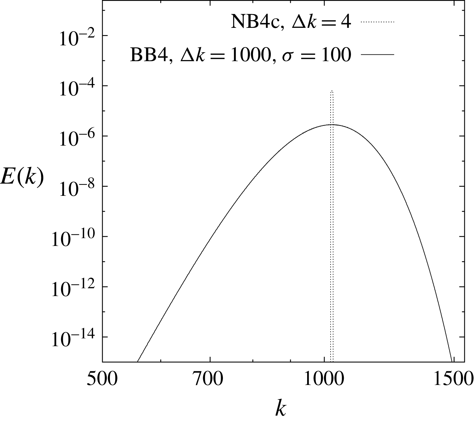
over one time step. The forcing spectra for narrowband and broadband forms with
 $k_{f}=1024$
are shown in figure 1.
Narrowband and broadband forcing spectra for runs NB4c and BB4 where
 $k_{f}=1024$
.

To examine the effect of finite forcing correlation time we use a Markovian time dependence obtained by first defining
 $$\begin{eqnarray}\displaystyle & \displaystyle \tilde{f}=r\hat{f}(\boldsymbol{k},t)+\sqrt{1-r^{2}}{\hat{c}}, & \displaystyle\end{eqnarray}$$
where
 $r=1-\text{d}t/f_{cr}$
and
 $f_{cr}$
is the forcing correlation radius, then defining
 $$\begin{eqnarray}\displaystyle & \displaystyle \hat{f}(\boldsymbol{k},t+\text{d}t)=\unicode[STIX]{x1D700}_{I}\,\text{d}t\,\tilde{f}/\langle \,\tilde{f}\hat{\unicode[STIX]{x1D713}}^{\ast }\rangle , & \displaystyle\end{eqnarray}$$
where
 $\langle \cdot \rangle$
denotes the average over the domain and
 $^{\ast }$
is the complex conjugate. The case
 $f_{cr}=0$
corresponds to
 $\unicode[STIX]{x1D6FF}$
-correlated forcing and
 $f_{cr}\rightarrow \infty$
corresponds to a forcing field that is constant in time.
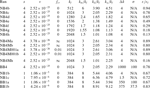
Table 1 contains parameters describing the various simulations. All are at resolution
 $8192^{2}$
, corresponding to
 $k_{m}=3072$
. The letters ‘NB’ and ‘BB’ denote narrowband and broadband forcing, respectively; the following number ‘1’ or ‘4’ denotes the order
 $s$
of the dissipation. The simulations with temporally correlated forcing are denoted ‘NB4M’, where M stands for ‘Markovian’. The values of the forcing correlation radius
 $f_{cr}$
are given in column 4.
Simulation parameters:
 $s$
is the order of viscosity,
 $\unicode[STIX]{x1D708}$
is the viscosity,
 $f_{cr}$
the forcing correlation radius,
 $k_{f}$
and
 $\unicode[STIX]{x0394}k$
the forcing wavenumber and bandwidth and
 $\unicode[STIX]{x1D70E}$
the variance of the Gaussian forcing envelope. For all simulations
 $N=8192$
and the maximum resolved wavenumber is
 $k_{m}=3072$
. The dissipation wavenumber
 $k_{d}$
is defined in (3.6), and
 $k_{\unicode[STIX]{x1D702}}$
is the wavenumber at which
 $\unicode[STIX]{x1D702}/k_{f}^{2}=0.5$
. The fraction of injected energy cascading to larger scales is
 $\unicode[STIX]{x1D700}/\unicode[STIX]{x1D700}_{I}$
.
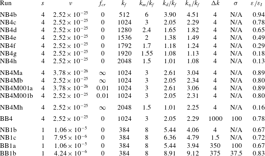
Columns 6–8 contain values for the forcing Reynolds number based on three alternative definitions. The simplest of these, in column 6, is the ratio of maximum resolved wavenumber to forcing wavenumber. Because this does not reflect the effects of varying order and strength of dissipation, it is useful to consider Reynolds numbers based on estimates of the dissipation wavenumber. One such estimate,
 $$\begin{eqnarray}\displaystyle & \displaystyle k_{d}=[\unicode[STIX]{x1D708}^{-3}k_{f}^{2}\unicode[STIX]{x1D700}]^{1/6s}, & \displaystyle\end{eqnarray}$$
where
 $\unicode[STIX]{x1D700}$
is the energy flux, was also used by Vallgren (Reference Vallgren2011) and Burgess et al. (Reference Burgess, Scott and Shepherd2015). The dissipation wavenumber may also be defined as the wavenumber
 $k_{\unicode[STIX]{x1D702}}$
at which the enstrophy flux
 $\unicode[STIX]{x1D702}/k_{f}^{2}$
falls to 0.5. Values of
 $k_{d}/k_{f}$
and
 $k_{\unicode[STIX]{x1D702}}/k_{f}$
are given in columns 7 and 8 of table 1.
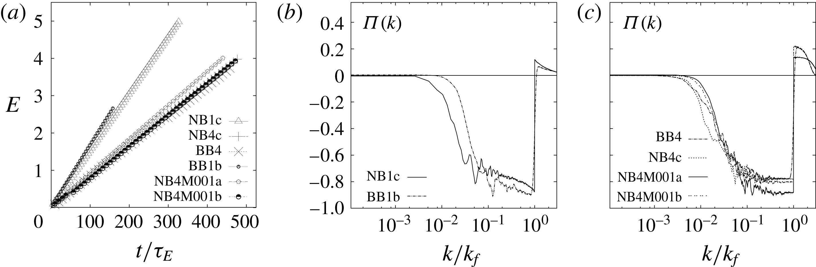
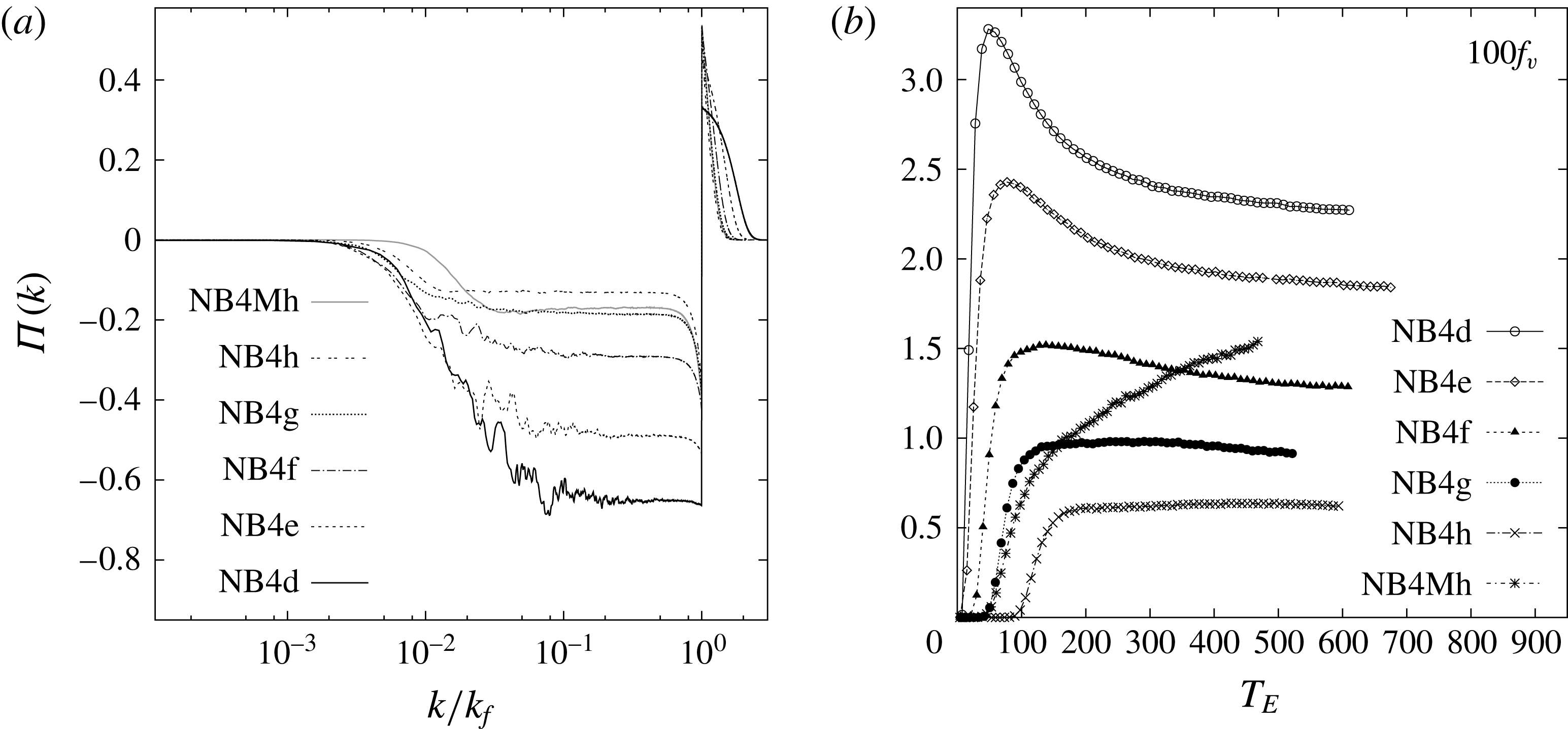
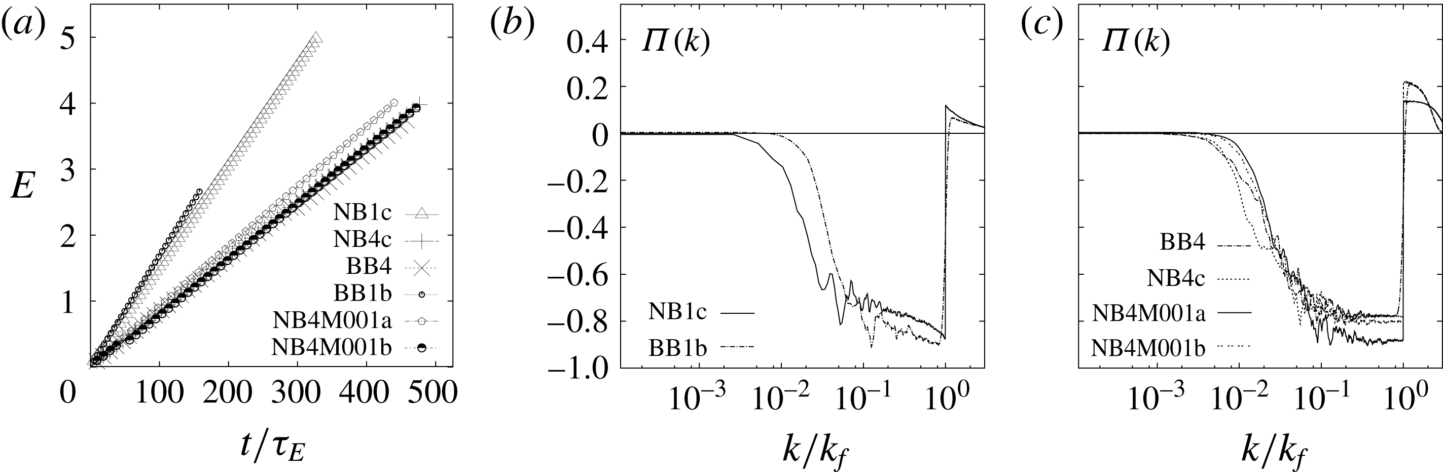
The total energy growth and energy flux in wavenumber space are shown in figure 2 for a selection of simulations. The energy is plotted as a function of a dimensionless time
 $t/\unicode[STIX]{x1D70F}_{E}$
, where
 $$\begin{eqnarray}\displaystyle & \displaystyle \unicode[STIX]{x1D70F}_{E}=(\unicode[STIX]{x1D700}k_{f}^{2})^{-1/3} & \displaystyle\end{eqnarray}$$
is a characteristic time associated with the enstrophy input rate, based on the energy flux
 $\unicode[STIX]{x1D700}$
to large scales (table 1, column 11). All cases show an approximately linear growth in energy (left) at a rate somewhat below the specified energy injection rate
 $\unicode[STIX]{x1D700}_{I}=1$
, the reduction resulting from non-zero energy loss to the small-scale dissipation. The reduction in energy growth rate is consistent with the plateau level in the energy fluxes (middle and right), which may be used as a measure of the strength of the inverse cascade in each simulation. In all cases shown, the forcing is well separated from the dissipation scales and most energy, typically over 70 %, cascades to larger scales (see table 1, column 11). In general, the inverse cascade is stronger at larger values of the forcing Reynolds number (table 1, columns 6–8). The plateaus in the hyperdiffusive cases (right) are flat over at least part of the inverse cascade because dissipation is effectively zero there. In contrast the broader spectral projection of the Laplacian diffusion (middle) means that dissipation has a small but persistent effect throughout the inverse cascade, resulting in decay of energy flux toward smaller
 $k$
. The effect of the broadband forcing, smoothing the sharp discontinuity at
 $k_{f}$
, can be seen most clearly in the flux for simulation BB1b, shown in the middle panel of figure 2.
Energy growth in time (a) and energy flux through
 $k$
-space (b,c) for a selection of cases (see table 1), illustrating the effects of broadband forcing, finite correlation times and Laplacian diffusion. There is a systematic dependence of the strength of the inverse cascade (magnitude of the plateau) on the forcing Reynolds numbers (table 1, columns 6–8). Fluxes have been averaged over 11 time steps centred on times
 $t=6.0$
for NB1c,
 $t=2.5$
for BB1b, and
 $t=5.0$
for the hyperviscous simulations.
4 Identification of coherent structures
As has been recognized for some time, identifying coherent structures in a turbulent flow is a highly non-trivial task. The definition of a ‘coherent vortex’ remains somewhat nebulous, but Haller et al. (Reference Haller, Hadjighasem, Farazmand and Huhn2016) specify two main requirements, namely that coherent vortices are concentrated regions of high vorticity, and that they propagate with a high degree of material invariance. It seems intuitively obvious that a vortex boundary must not only enclose an intense concentration of vorticity, it must also consist of the same material fluid elements at all times, otherwise the classification of fluid elements as falling within or outside the vortex will fluctuate, contrary to the notion of coherence. Vortex identification methods that are not based on material invariants will in general not consistently identify the same set of fluid elements as the vortex boundary at all times. Such criteria include the Okubo–Weiss criterion (Okubo Reference Okubo1970; Weiss Reference Weiss1991) and its refinement, the Hua–Klein criterion (Hua & Klein Reference Hua and Klein1998), which involve the eigenvalues of the velocity and acceleration gradient tensors, respectively.
In two-dimensional inviscid flows governed by the Euler equation vorticity is frozen into the flow, meaning that a fluid parcel maintains its initial value of vorticity for all times. This material invariance makes vorticity isolines attractive and obvious candidates for vortex boundaries in the large Reynolds number limit
 $Re\rightarrow \infty$
. As long as the effects of dissipation are negligible, a given vorticity threshold is guaranteed to identify the same set of fluid elements at all times. In fact, the vortex identification method proposed in Haller et al. (Reference Haller, Hadjighasem, Farazmand and Huhn2016) involves applying a threshold to the Lagrangian-averaged vorticity deviation (LAVD), the trajectory integral of the normed difference between the fluid element’s vorticity and the spatial mean vorticity. In a two-dimensional flow with zero mean vorticity and negligible viscous effects (which we expect to apply in vortex cores and on their boundaries), thresholding on the LAVD is equivalent to thresholding on the instantaneous vorticity.
The controversy surrounding the definition of a ‘vortex’ is perhaps best understood as an instance of a broader problem, namely identifying the correct extended physical space objects with which to describe turbulence. Here, we understand ‘correct’ to mean variables that will yield an elegant description of the flow. As discussed in § 2.2, there are strong theoretical reasons to expect that isolines of vorticity and their enclosed regions will play an important role in the description of two-dimensional turbulence. These theoretical considerations motivate our definition of a vortex area as an intense vorticity concentration bounded by a level set of vorticity. In testing our theory, the vortex identification method should reflect the same principles, and this consideration leads naturally to an identification method based on a vorticity threshold.
We used two thresholding procedures to identify vortex areas. The first involves a single threshold, together with restrictions on eccentricity and the peak value of vorticity within the region. The latter restriction is intended to ensure that the region is an intense vortex. We also used a multi-level thresholding procedure with a base cutoff
 $\unicode[STIX]{x1D714}_{thr}$
. This procedure is more complex than the single threshold used by Burgess & Scott (Reference Burgess and Scott2017), and is designed to remove strong filaments from coherent structures in the Laplacian runs, where intensities within vortices and their trailing filaments are comparable. In practice, though the multi-level threshold yields vortex fields that appear cleaner upon visual inspection, it has a negligible effect on the number density and vortex growth rate as compared to a single stage threshold.
The results presented below are for the multi-level threshold algorithm, which begins by identifying regions for which
 $\unicode[STIX]{x1D714}\geqslant \unicode[STIX]{x1D714}_{thr}$
, and discarding those that fall below a minimum allowed size
 $A_{min}=\unicode[STIX]{x03C0}r_{min}^{2}$
, where
 $r_{min}=\unicode[STIX]{x03C0}/(k_{f}+\unicode[STIX]{x1D70E})$
, and
 $\unicode[STIX]{x1D70E}$
is as defined in table 1. It also discards regions for which the peak value of the vorticity within the region does not exceed a second threshold
 $\unicode[STIX]{x1D714}_{thr}^{p}$
; the purpose of this threshold is to ensure that regions selected are in fact intense vortices. Within a wide range of values, the choice of
 $\unicode[STIX]{x1D714}_{thr}^{p}$
has little effect on the vortex populations selected in the hyperviscous runs, whereas it has a more significant effect on the populations and corresponding densities in the Laplacian runs, which is not surprising given the lesser intensity difference between the vortices and surrounding field in these simulations; we discuss this below in § 5. For the narrowband simulations,
 $\unicode[STIX]{x1D70E}$
is the parameter chosen for the corresponding broadband run. The eccentricity
 $$\begin{eqnarray}\displaystyle & \displaystyle e=\sqrt{1-{\displaystyle \frac{\unicode[STIX]{x1D706}_{2}}{\unicode[STIX]{x1D706}_{1}}}} & \displaystyle\end{eqnarray}$$
of the region is then calculated, with
 $\unicode[STIX]{x1D706}_{1}$
and
 $\unicode[STIX]{x1D706}_{2}$
the eigenvalues of the covariance matrix formed from the second-order moments of
 $\unicode[STIX]{x1D714}$
(e.g. Liu & Scott Reference Liu and Scott2015, section 2.5). Structures with
 $e<0.9$
are retained, i.e. removed from the original vorticity field and stored in a coherent field; this value of
 $e$
was chosen by examining the resulting coherent field to ensure that almost all vortices were selected while eliminating filaments in the Laplacian runs. (The eccentricity criterion has little to no effect on the hyperviscous coherent fields.) The threshold is then increased to
 $\unicode[STIX]{x1D714}_{thr}+(\unicode[STIX]{x1D714}_{max}-\unicode[STIX]{x1D714}_{thr})/n_{lev}$
, where
 $\unicode[STIX]{x1D714}_{max}$
is the vorticity extremum at that time, and we take
 $n_{lev}=1000$
levels. The selection procedure is then repeated until the largest identified structure falls below the minimum allowable size, at which point the search algorithm terminates. Removing the qualifying coherent structures from the field at each level ensures that no regions are double-counted.
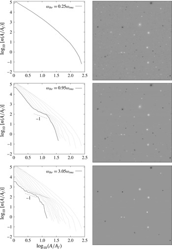
Vortex number density distributions (left) and corresponding anomaly fields for thresholds on vorticity from
 $0.25\unicode[STIX]{x1D714}_{rms}$
to
 $3.05\unicode[STIX]{x1D714}_{rms}$
. The data used are from simulation NB4c at
 $t/\unicode[STIX]{x1D70F}_{E}=467$
.

Because the choice of
 $\unicode[STIX]{x1D714}_{thr}$
is somewhat arbitrary, we have performed a threshold sensitivity study for the simulation NB4c. We utilize a single threshold with values in between
 $0.25\unicode[STIX]{x1D714}_{rms}$
and
 $3.05\unicode[STIX]{x1D714}_{rms}$
to explore the dependence of the number density distribution of vortex areas on the threshold. The results are shown in figure 3 for dimensionless time
 $t/\unicode[STIX]{x1D70F}_{E}=467$
, with the number density on the left and the corresponding vortex field on the right. As is evident, the three-part number density emerges just as the threshold becomes high enough to isolate nearly circular intense vortices. Moreover, the power laws of the scaling ranges remain virtually unchanged for thresholds between
 $0.95\unicode[STIX]{x1D714}_{rms}$
and
 $3.05\unicode[STIX]{x1D714}_{rms}$
. (The threshold can be taken higher, but the statistics become increasingly noisy and the ‘thermal bath’ shallows as more and more vortex areas fail the minimum size criterion.) The emergence of the three-part number density as the threshold identifies circular, intense, long-lived vortices justifies the association of these scaling ranges with the coherent vortex population. The insensitivity of the number density to the threshold once long-lived vortices are identified shows that the scaling form equation (2.23) is a robust result not limited to a special choice of cutoff.
We note that there is an observable relationship between the intensity of the vorticity concentration enclosed by an isoline and its tendency to avoid deformation and filamentation. In general, the stronger the circulation of the region enclosed relative to the background flow, the more circular and smooth the isoline. This can be seen by comparing the right middle and lower panels in figure 3: in the lower panel the threshold is higher and the structures all have unfilamented boundaries. Hence, the problem of selecting appropriate material curves as vortex boundaries is not independent from the problem of ensuring that those boundaries enclose vorticity concentrations.
In most of the simulations reported below, we have used parameter values
 $\unicode[STIX]{x1D714}_{thr}=1.5\unicode[STIX]{x1D714}_{rms}$
,
 $\unicode[STIX]{x1D714}_{thr}^{p}=4\unicode[STIX]{x1D714}_{rms}$
and
 $e_{max}=0.9$
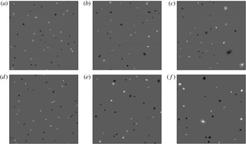
. Examples of the resulting coherent vorticity fields are illustrated in figure 4 for cases with broadband forcing and Laplacian diffusion (a–c) and hyperdiffusion (d–f). Only a small portion of the full domain is shown, the subdomains having the same resolution with respect to the forcing scale,
 $(48l_{f})^{2}$
, where
 $l_{f}=8192/k_{f}$
is the forcing length scale in number of grid sites. This corresponds to regions of size
 $384^{2}$
grid points (
 $0.22\,\%$
of the domain) for the case BB4 and
 $1024^{2}$
grid points (
 $1.56\,\%$
of the domain) for the case BB1a.
Since other vortex identification methods, including the Okubo–Weiss and Hua–Klein criteria, extract regions of the flow with different characteristics, one would, in general, expect the statistics of these regions to differ from those of the areas bounded by isolines considered here. The dependence of the statistics on the extraction method is an interesting question, and might provide insight into the structure of vortices. However, such a study is beyond the scope of this paper.
5 The vortex population at moderate forcing Reynolds number
The fields shown in figure 4 illustrate both the nature of the dilute vortex populations across spatial scales and their evolution in time. Times are selected at comparable values of the quantity
 $l_{\unicode[STIX]{x1D714}}/l_{f}$
, so that top and bottom rows represent similar stages of evolution in the vortex population. The vorticity fields of both simulations are populated by intense quasi-circular structures that persist in time, grow through merger and span a broad range of sizes, signalling a hierarchical population, as will be discussed shortly. Careful inspection, in particular of the rightmost panels, indicates a rougher and more filamentary field in the Laplacian (top row) than in the hyperdiffusive (bottom row) simulation. The more coherent structure of vortices in the hyperdiffusive case possibly reflects the tendency of hyperdiffusion to develop overshoots in vorticity profiles, leading eventually to anomalously intense vortices. Aside from this difference, it is clear that both cases have developed a dilute field of coherent vortices spanning a range of scales well above the scale of the forcing. It is difficult to distinguish any difference between (f) and the corresponding narrowband, hyperdiffusive case analysed in figure 2(b) of Burgess & Scott (Reference Burgess and Scott2017), showing that the vortex formation is not an artefact of the narrowband forcing used in that study.
Coherent vorticity fields for the broadband Laplacian simulation BB1a on a
 $1024^{2}$
subdomain (1.56 % of the domain) at
 $t=2.2,3.7,5.8$
(a–c), and for the broadband hyperviscous simulation BB4 on a
 $384^{2}$
(0.22 % of the domain) subdomain at
 $t=1.0,1.9,3.1$
(d–f). Both subdomains have side lengths
 $48l_{f}$
, where
 $l_{f}$
is the forcing length scale, and the times are chosen such that
 $l_{\unicode[STIX]{x1D714}}/l_{f}=0.00092,0.0012,0.00148$
(left to right) in both simulations.

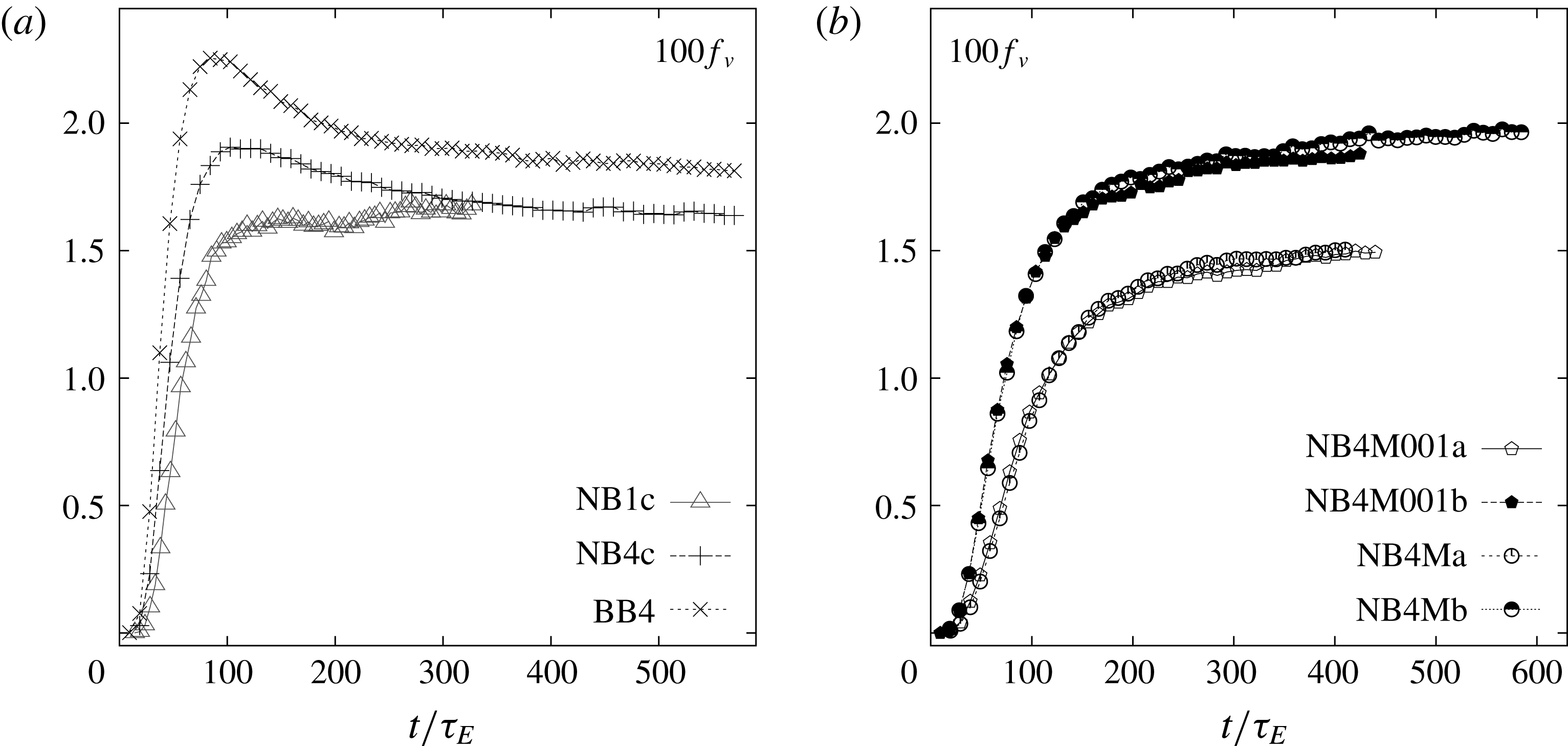
Percentage
 $100f_{v}$
of the domain occupied by coherent vortices. (a) Simulations NB1c, NB4c, BB4. (b) Simulations NB4M001a, NB4M001b, NB4Ma, NB4Mb.

Figure 5 shows the percentage of the domain,
 $100f_{v}$
, occupied by coherent vortices, where
 $f_{v}$
is as defined in (2.25). In panel (a) we compare the case NB4c studied by Burgess & Scott (Reference Burgess and Scott2017) with cases NB1c and BB4. At early times,
 $t<2$
, the vortex population has not fully developed. Once the vortices have emerged, all three cases show a tendency toward a constant area fraction
 $f_{v}$
, as predicted by Burgess & Scott (Reference Burgess and Scott2017) and discussed in § 2. In both hyperdiffusive cases the area fraction
 $f_{v}$
overshoots and peaks at a higher value than the one at which it equilibrates, whereas in the diffusive case there is a more monotonic increase to the final value. The early time difference may be due to the effect of different diffusion operators on the initial vortex formation, or possibly reflects inaccuracies in the vortex extraction algorithm when applied to the early time fields, the extraction being designed primarily with the aim of accurately capturing coherent structures once the vortex population is developed.
Figure 5(b) shows a selection of cases with finite forcing decorrelation time, in particular the cases
 $f_{cr}=0.01$
and
 $f_{cr}=\infty$
. The former forcing choice may be considered a smoothing of
 $\unicode[STIX]{x1D6FF}$
-correlated forcing on a time scale that is still short compared to the time scale for vortex motions. The latter is the more extreme case in which the forcing field is constant in time (though still spatially random). Two simulations of each case are shown with different forcing Reynolds number, which has the effect of changing the overall area fraction; this dependence is examined in more detail in § 6 below. A comparison with figure 5(a) indicates that the introduction of even a short decorrelation time alters the early time formation of the vortex field. However, it is interesting that further increases in the decorrelation time have virtually no effect on the coherent area fraction development.
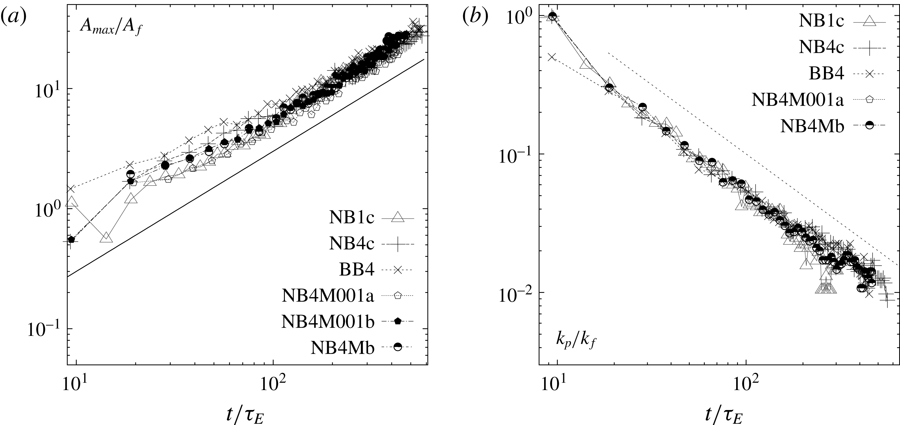
The area of the largest vortex,
 $A_{max}$
and the wavenumber of the peak of the energy spectrum,
 $k_{p}$
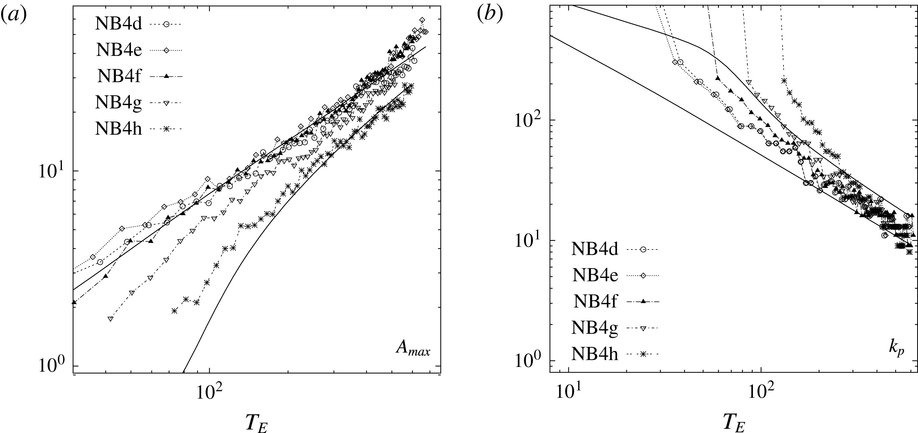
, are shown in figure 6. The area of the largest vortex (figure 6
a) follows the growth law
 $A_{max}\sim t$
predicted by Burgess & Scott (Reference Burgess and Scott2017) and derived in § 2. To collapse the curves we have plotted
 $A_{max}$
normalized by the forcing scale area
 $A_{f}$
and as a function of a rescaled dimensionless time
 $t/\unicode[STIX]{x1D70F}_{E}$
. Despite some noise, the growth rate is well supported in all cases. Similarly, the spectral peak evolution (figure 6
b) also follows the predicted
 $k_{p}\sim t^{-1}$
law in all five simulations plotted. In addition to following the predicted growth rates, the results indicate that the constant of proportionality is very similar across all cases, for both
 $A_{max}/A_{f}$
and
 $k_{p}/k_{f}$
.
(a) Area of the largest vortex normalized by the forcing area,
 $A_{max}/A_{f}$
, for simulations Nb1c, NB4c, BB4 and NB4M; the solid line has slope
 $t^{1}$
. (b) Wavenumber of the spectral peak normalized by the forcing wavenumber
 $k_{p}/k_{f}$
for the same simulations; the dotted line has slope
 $t^{-1}$
. Both quantities are plotted as a function of dimensionless time
 $t/\unicode[STIX]{x1D70F}_{E}$
.

We next consider in more detail the evolution of the characteristic wavenumbers
 $k_{\unicode[STIX]{x1D714}}$
and
 $k_{E}$
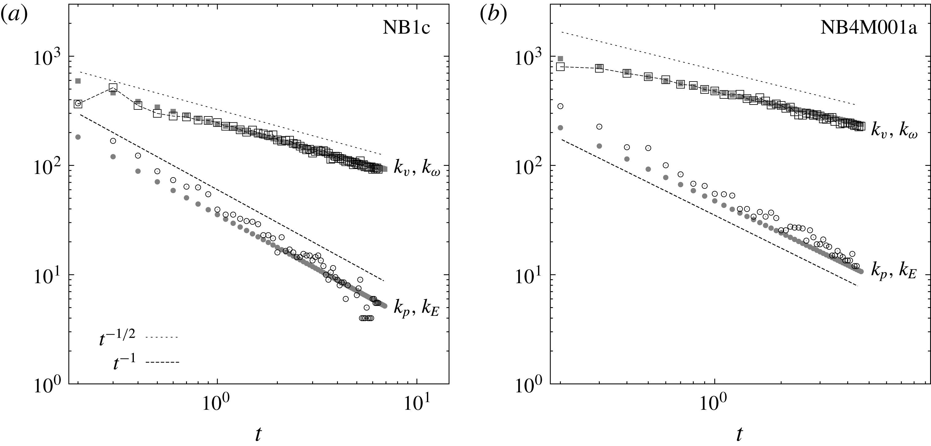
defined in § 2.1, equations (2.12) and (2.14), respectively. For this purpose we select simulations NB1c with Laplacian diffusion and NB4M001a with non-zero forcing decorrelation time scale. The maximum vortex size as shown in figure 6 is associated with a vortex wavenumber
 $k_{v}=\unicode[STIX]{x03C0}/\sqrt{A_{max}/\unicode[STIX]{x03C0}}$
that may be compared with the wavenumber
 $k_{\unicode[STIX]{x1D714}}$
. Similarly, we compare the energy spectral peak wavenumber
 $k_{p}$
with the characteristic wavenumber
 $k_{E}$
. All four wavenumbers are shown in figure 7 for NB1c (a) and NB4M001a (b). The wavenumbers
 $k_{\unicode[STIX]{x1D714}}$
(▪, grey) and
 $k_{E}$
(+), being defined from the bulk quantities
 $E$
and
 $Z$
, are well constrained and follow the expected
 $t^{-1/2}$
and
 $t^{-1}$
evolution with good agreement. The wavenumber
 $k_{v}$
(▫) associated with the largest vortex also follows the predicted
 $t^{-1/2}$
decay law well, and coincides very well with the characteristic wavenumber
 $k_{\unicode[STIX]{x1D714}}$
. The measured spectral peak wavenumber
 $k_{p}$
(○) is noisier, especially in simulation NB1c, where the spectral peak is closer to the domain scale, but still follows the predicted
 $t^{-1}$
decay reasonably well. A similar agreement between measured and predicted growth rates was found for cases with broadband forcing and other choices of forcing and dissipation.
Characteristic and empirical wavenumbers for the Laplacian simulation NB1c (a) and the Markovian simulation NB4M001a (b) together with predicted growth laws. Grey symbols denote the characteristic wavenumbers
 $k_{\unicode[STIX]{x1D714}}$
and
 $k_{E}$
.

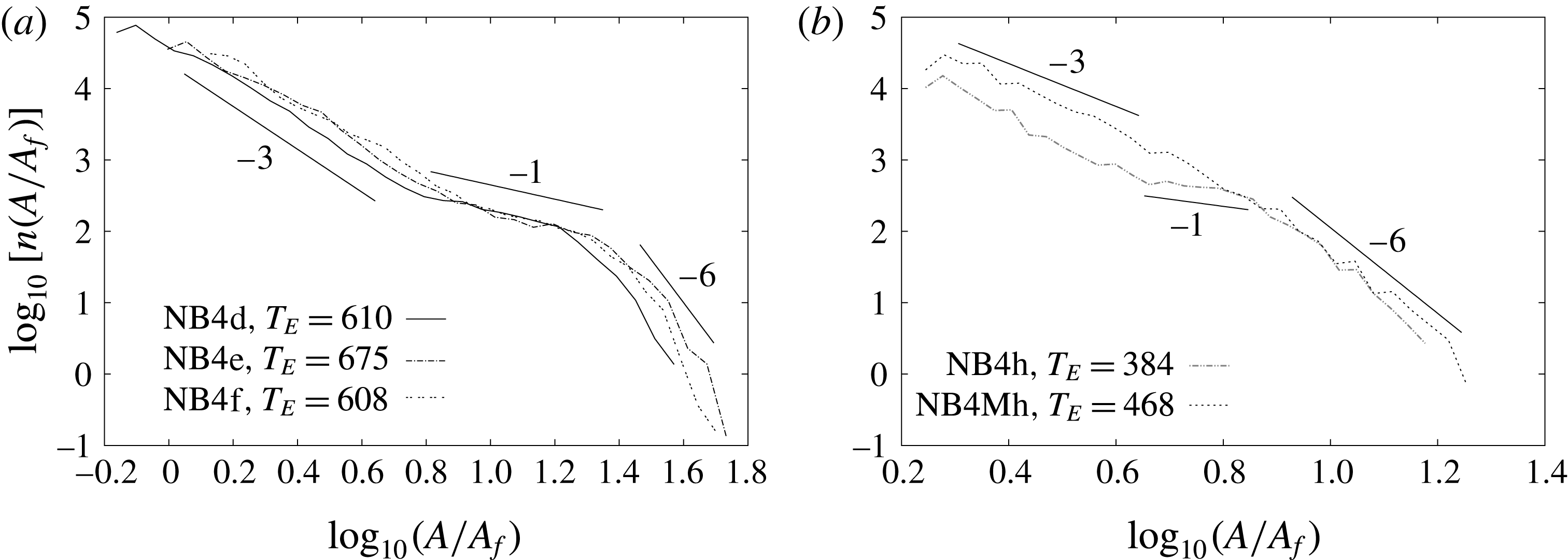
The vortex number density
 $n(A/A_{f})$
, normalized by the total vortex number
 $N$
, is shown in figure 8 for a selection of simulations; the case NB4c with narrowband,
 $\unicode[STIX]{x1D6FF}$
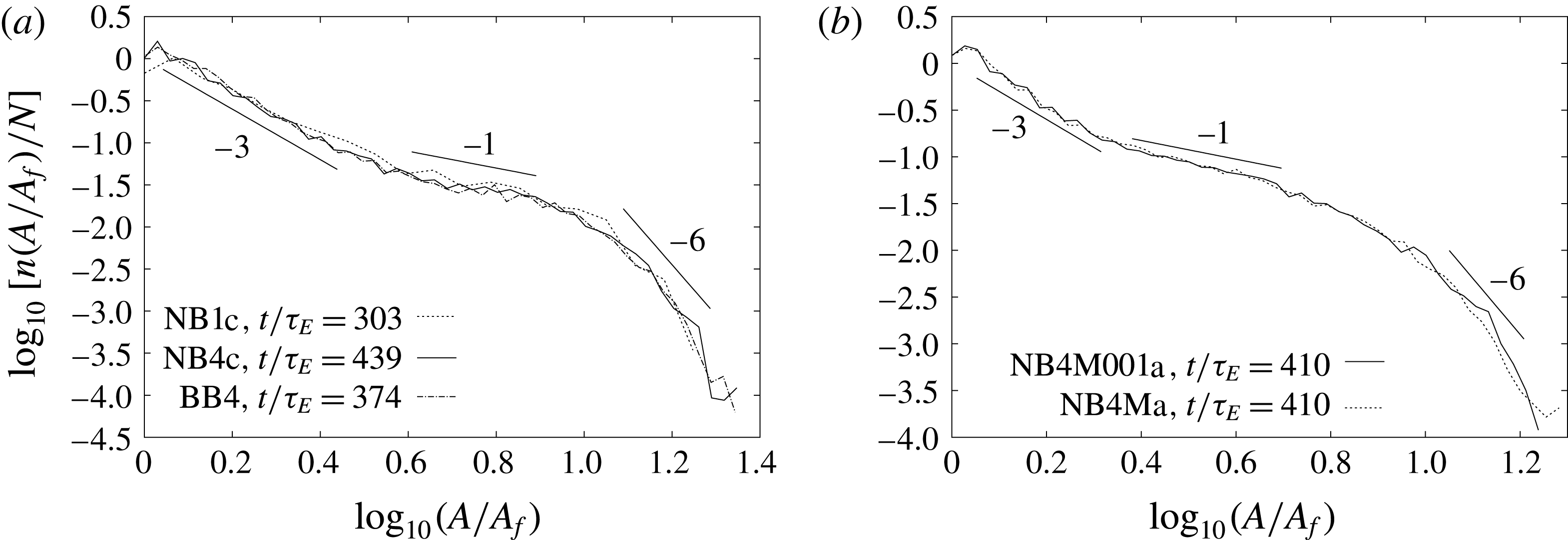
-correlated forcing and hyperviscous dissipation considered in Burgess & Scott (Reference Burgess and Scott2017) appears in (a) (solid line). The times are chosen so that the vortex population has developed to a comparable stage in each simulation. Two main features are worth noting. First, the cases BB4 and NB1c, each similar to NB4c, except for the use of broadband forcing and Laplacian dissipation, respectively, exhibit nearly identical vortex number densities to the NB4c simulation. In all cases the number density takes the three-part form described in § 2, with approximate slopes of
 $-3$
,
 $-1$
and
 $-6$
. The evidence for power law scaling is weakest in the steep large-scale range three, but as shown in Burgess & Scott (Reference Burgess and Scott2017) the conservation properties of this range are distinct from ranges one and two, and consistent with the arguments of (intensity-weighted) number conservation used to derive the number density in this range. This suggests that even if range three lacks clean power law scaling, it is dynamically distinct from the other two ranges. Other simulations show similar behaviour, and no significant differences were found in simulation BB1, in which both broadband forcing and Laplacian diffusion are used in combination. Thus, the first conclusion we draw here is that the vortex population obtained in Burgess & Scott (Reference Burgess and Scott2017) is not particularly sensitive to either the spectral bandwidth of the forcing, or to the order
 $s$
of viscous dissipation.
The second point illustrated in figure 8 is a small but significant effect of forcing decorrelation time on the vortex population. In (b), we show the vortex number densities for simulations NB4M001a and NB4Ma at non-dimensional time
 $t/\unicode[STIX]{x1D70F}_{E}=410$
. For NB4M001a the decorrelation time scale is
 $f_{cr}=0.01$
, which in terms of the rescaled time is approximately unity (
 $\unicode[STIX]{x1D70F}_{E}\approx 0.01$
): the forcing time scale for this case is thus comparable to the dynamical time scale, but still much shorter than the time scale on which the vortex population as a whole evolves. For the case NB4Ma, the decorrelation time scale is infinite, corresponding to the extreme case of forcing that is steady in time. From the figure, it is clear that in both cases nearly identical vortex populations have emerged. While again they exhibit three distinct scaling ranges with approximately the predicted slopes, the overall shape of the population shows some differences from the NB4c case. In particular, the
 $-3$
thermal bath range is shorter, the intermediate-range slope is slightly steeper than
 $-1$
at this time and the transition from the intermediate range to the large-scale
 $-6$
range occurs more slowly, i.e. over a broader range of scales in vortex area. We note that the steepening past a
 $-1$
slope in the intermediate scaling range occurs at later stages of the flow evolution, as is evident from figure 9(c,d), where a
 $-1$
slope can be seen at earlier times. The origin of these differences is not clear but we offer some speculations in § 7 below. Here, we note that the steeper intermediate range appears to be related to the forcing Reynolds number: reducing this further (simulation NB4Mb, not shown) has the effect of steepening the slope even more. Overall, it appears that the introduction of a non-zero decorrelation time of the order of the dynamical time scale may alter the vortex population while preserving the basic three-part structure of the number density, but that further increase in the forcing time scale has no discernible effect.
Number densities normalized by total vortex number
 $N$
for simulations NB1c, NB4c and BB4 (a) and NB4Ma and NB4M001a (b).

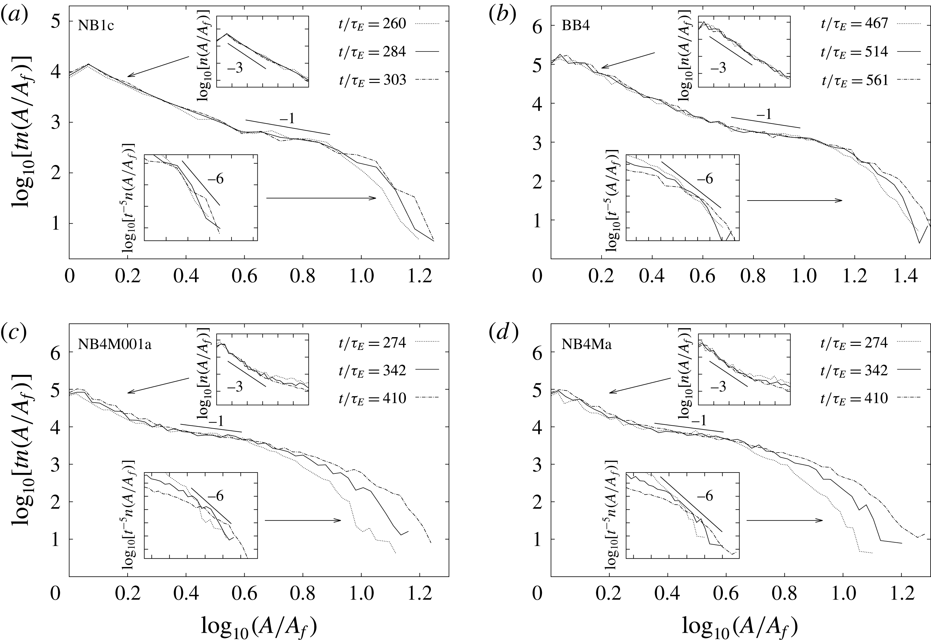
Number densities at the indicated times for simulations NB1c (a), BB4 (b), NB4M001a (c) and NB4Ma (d). The main panels show
 $tn(A/A_{f})$
, the upper insets show
 $n(A/A_{f})$
and the lower insets show
 $t^{-5}n(A/A_{f})$
.

The time evolutions of the number densities for the same four simulations are shown in figure 9. The main panels show the densities compensated by a factor of
 $t$
which, as found in Burgess & Scott (Reference Burgess and Scott2017) for simulation NB4c, collapses the curves fairly well in the intermediate range. Likewise, the
 $A^{-3}$
thermal bath ranges are all approximately constant in time (upper insets). Thus, while the non-zero forcing decorrelation time of the NB4M cases has shortened this range with respect to the NB4, BB4, NB1 cases, both the area and time dependence appear relatively unchanged. Finally, although the large-scale ranges are difficult to measure because of the relative scarcity of vortices at these scales, the
 $t^{-5}$
temporal rescaling results in a reasonable collapse of the data in this range (lower insets). Again, the evidence for power law scaling and collapse of the curves is weakest at the largest scales, but consistent with the constraint between the spatial and temporal scaling exponents based on number conservation. Thus, the predictions (2.23) for both the area and time dependence are reasonably well supported in all cases and show little sensitivity to the details of the forcing and dissipation.
Vortex intensities
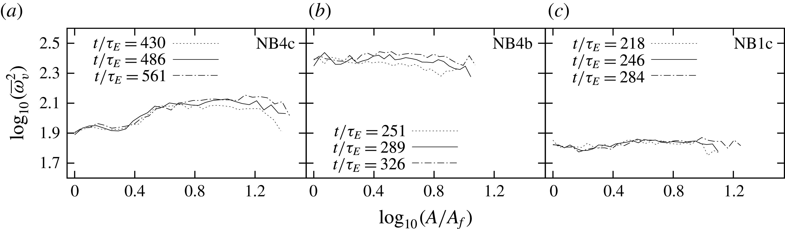
 $\overline{\unicode[STIX]{x1D714}_{v}^{2}}$
at three times for simulations NB4c (
 $k_{f}=1024$
, a), NB4b (
 $k_{f}=512$
, b) and NB1c (c).

As discussed in Burgess & Scott (Reference Burgess and Scott2017), the predictions (2.23) are based on the assumption that the vortex intensity
 $\overline{\unicode[STIX]{x1D714}_{v}^{2}}$
is independent of both area and time. While constancy across area was well supported by the numerical simulations in that study, a systematic growth in
 $\overline{\unicode[STIX]{x1D714}_{v}^{2}}$
was observed and related to departures of the number density’s temporal evolution from the predicted growth rates. We plot the vortex intensities
 $\overline{\unicode[STIX]{x1D714}_{v}^{2}}$
in figure 10 with equal scales on the vertical and horizontal axes to accurately convey the variation with vortex area
 $A$
. The ensemble of simulations analysed in Burgess & Scott (Reference Burgess and Scott2017) was equivalent in terms of parameters to NB4c, for which
 $\overline{\unicode[STIX]{x1D714}_{v}^{2}}$
is shown in figure 10(a) at a series of times, illustrating the growth in time of
 $\overline{\unicode[STIX]{x1D714}_{v}^{2}}$
in both the intermediate and large-scale ranges. All simulations listed in table 1 with moderate Reynolds number and hyperviscous dissipation exhibit a similar growth in
 $\overline{\unicode[STIX]{x1D714}_{v}^{2}}$
, though we have not attempted to determine the growth rates in the intermediate and large-scale ranges of the number density, as was done in Burgess & Scott (Reference Burgess and Scott2017). There is some variation of
 $\overline{\unicode[STIX]{x1D714}_{v}^{2}}$
with
 $A$
, which can be traced to the effects of dissipation: in panel (b) we include vortex intensities from a simulation labelled NB4b, which has the same parameters as NB4c, but is forced at larger scales (
 $k_{f}=512$
as opposed to
 $k_{f}=1024$
for NB4c). As can be seen by comparing panels (a) (NB4c) and (b) (NB4b), the dependence of vortex intensity on area reflects the choice of dissipation mechanism only insofar as the order of dissipation controls how rapidly diffusive effects fall off with
 $A$
across the vortex-containing scales. This effect is more pronounced for the hyperviscous simulation NB4c, which is forced at scales where dissipative effects are still appreciable. The noticeable variation of vortex intensity with
 $A$
is due to the fact that diffusive effects fall off much more quickly with increasing length scale for hyperviscosity than they do for the ordinary Laplacian diffusion used in simulation NB1c. The variation of vortex intensity with area can be eliminated from the hyperviscous simulations by forcing at larger scales, or, equivalently, in still higher resolution calculations in which the effect of dissipation is moved to smaller scales. This shows that the shape of the number density is not particularly sensitive to the diffusive effects seen in the plot of vortex intensity as a function of area for NB4c. At earlier times
 $\overline{\unicode[STIX]{x1D714}_{v}^{2}}$
also grows in the Laplacian simulations, but at these times the intermediate scale-invariant
 $-1$
range has not yet been established. At later times, once this range has been established,
 $\overline{\unicode[STIX]{x1D714}_{v}^{2}}$
equilibrates in the narrowband Laplacian simulations. This differs from the hyperviscous simulations, in which
 $\overline{\unicode[STIX]{x1D714}_{v}^{2}}$
keeps growing at intermediate scales even though the
 $-1$
range has already been established. As an example, we show the case NB1c in figure 10(c); other Laplacian simulations show similar constancy in time. We note that the effect of viscosity on the vortex population is much stronger in NB1c, as can be deduced from the attenuation of the flux with scale, evident in figure 2(b). It is thus not immediately clear whether the lack of growth in
 $\overline{\unicode[STIX]{x1D714}_{v}^{2}}$
seen in NB1c is due to absence of hyperviscous sharpening, or to increased dissipative effects balancing the enstrophy input into the range. Nonetheless, the growth of
 $\overline{\unicode[STIX]{x1D714}_{v}^{2}}$
observed in Burgess & Scott (Reference Burgess and Scott2017) is evidently non-robust, and sensitive to the form and/or strength of the diffusion.
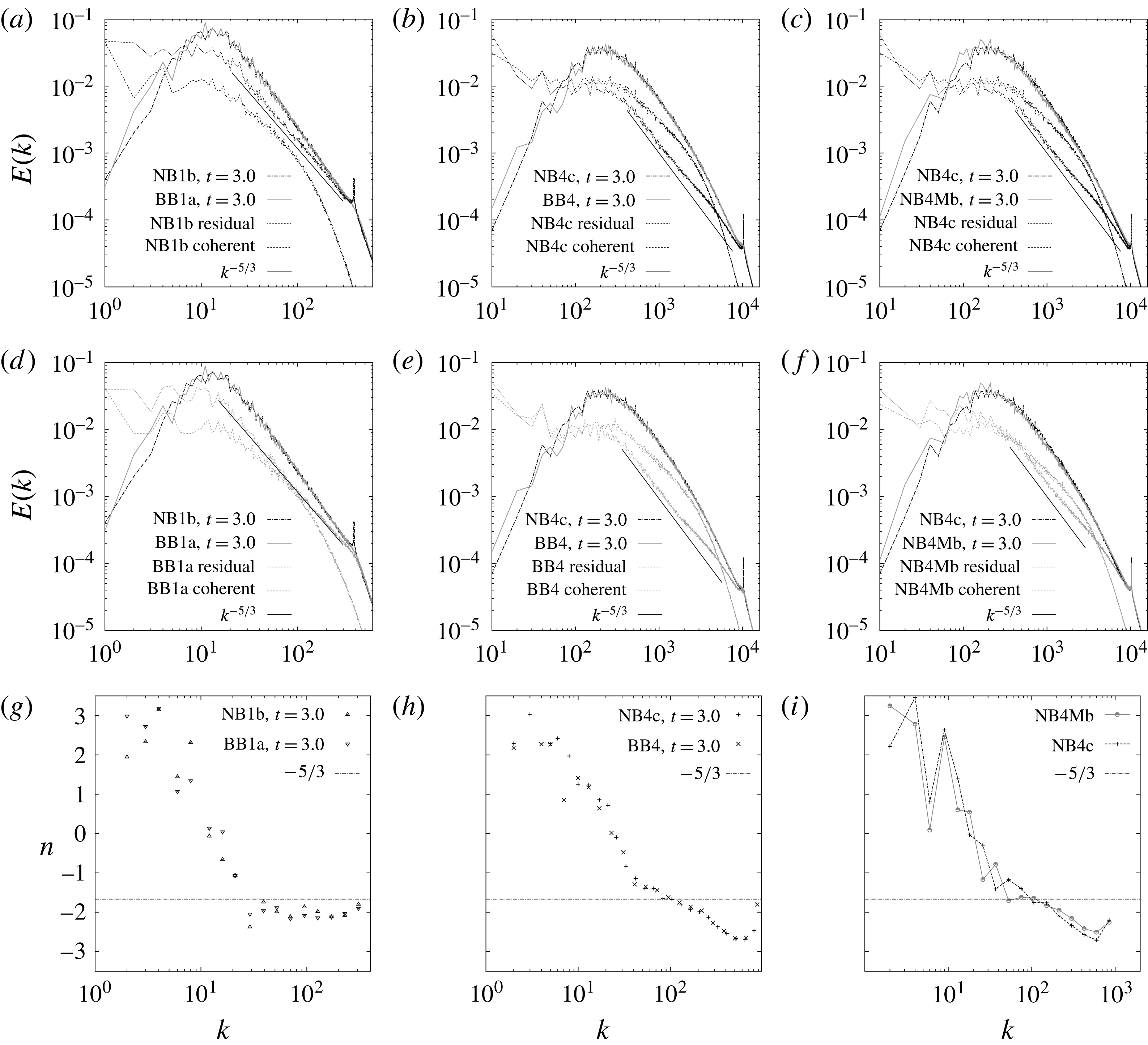
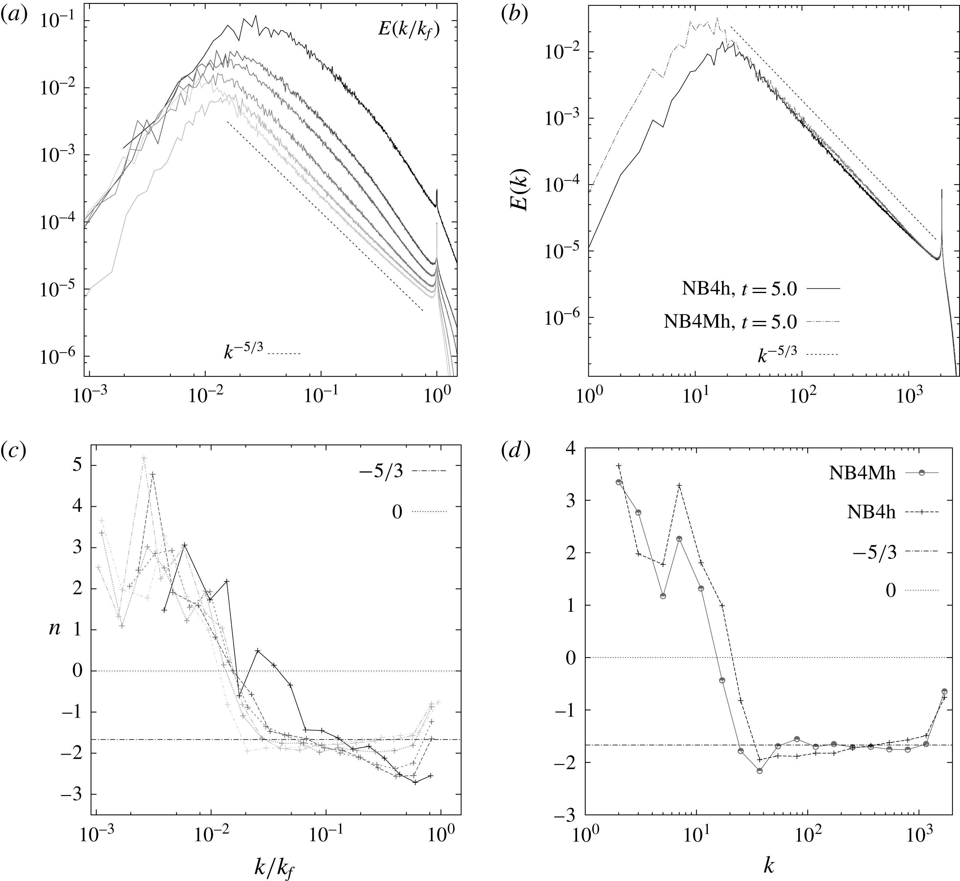
Energy spectra for Laplacian (a,d,g), hyperviscous
 $\unicode[STIX]{x1D6FF}$
-correlated (b,e,h) and hyperviscous
 $\unicode[STIX]{x1D6FF}$
-correlated and constant forcing simulations (c,f,i) with intermediate-range forcing. In (a–f) total spectra for two simulations are shown together with coherent and residual spectra for one of the simulations. For example, in (a) total spectra for NB1b and BB1a are shown together with coherent and residual spectra for simulation NB1b, while directly below in (d) total spectra for NB1b and BB1a are shown again together with coherent and residual spectra for simulation BB1a for comparison. In the bottom row are shown corresponding local slopes for the total energy spectra averaged over equal intervals in
 $\text{log}(k)$
.

Finally, figure 11 shows energy spectra for the Laplacian simulations NB1b and BB1a (a) and (d), hyperviscous simulations with
 $\unicode[STIX]{x1D6FF}$
-correlated forcing NB4c and BB4 (b) and (e) and the hyperviscous simulations NB4c and NB4Mb with
 $\unicode[STIX]{x1D6FF}$
-correlated and infinitely correlated forcing, respectively, and equal values of dissipation (c) and (f). Each of panels (a–f) shows total spectra (i.e. of the unfiltered fields) from two simulations, together with coherent and residual spectra from one of the simulations; the spectra for the other simulation are shown immediately below. Panels (a) and (d) both show total spectra from simulations NB1b and BB1a; coherent and residual spectra for NB1b are shown in (a), while coherent and residual spectra for BB1a are shown in (d). Similarly, (b) and (e) show spectra from simulations NB4c and BB4, while (c) and (f) show spectra from simulations NB4c and NB4Mb. The coherent spectra shown are for fields obtained via the extraction procedure described in § 4.
Considering first the total spectra, the choice of narrowband versus broadband forcing has no impact on the spectrum in the inverse cascade sufficiently far above the peak forcing wavenumber, as is evident in (a,b), which compare simulations NB1b to BB1a and NB4c to BB4, respectively, and in the corresponding local slope (g,h). There is a small but noticeable difference in the spectral slopes between the simulations NB4c and NB4Mb with delta-correlated and infinitely correlated forcing, respectively, which is most evident in the local slope plot in (i). By far the biggest differences in energy spectra lie in the comparison between Laplacian and hyperviscous dissipation, as can be seen by comparing (g) to (h,i). Consistent with previous studies (Scott Reference Scott2007; Vallgren Reference Vallgren2011; Fontane et al.
Reference Fontane, Dritschel and Scott2013) we find a slope of approximately
 $-2$
in the Laplacian simulations, illustrated by the local slopes in (g), which are around
 $-2$
up to
 $k=30$
and then shallow slowly. In contrast, the local slope in the hyperviscous simulations is much less constant above the forcing scale, such that there is no clear power law, as shown in (h,i).
Considering now the coherent and residual spectra, the vorticity field can be decomposed into an incoherent filamentary subfield with an energy spectrum
 $E(k)\sim k^{-5/3}$
, in accordance with the Kraichnan theory, and a coherent subfield whose energy spectrum shows a more complex dependence with no clear power law. The coherent spectrum is rounded, with a shallower dependence at moderate wavenumbers, and a rapid fall-off just above the forcing scale. The energy spectra of the complete unfiltered vorticity fields arise from the combination of the coherent spectrum, with its rounded shape and very rapid decrease, and the
 $k^{-5/3}$
power law dependence of the background spectrum.
It is notable that the vortical area distribution, as captured by the number densities in figures 8 and 9, shows a higher degree of universality than the energy spectra in figure 11. One reason for this is that the power in the coherent field relative to the residual background field varies depending on the simulation parameters: in simulations NB4c and BB4 shown in (b) and (e) there is more power in the coherent field, while in simulations NB1b and BB1a shown in (a) and (d) there is more power in the residual field. This difference in relative power explains why the spectral shape depends on the simulation parameters, while the number density distribution is relatively universal. Fully explaining the shape of the observed total spectrum would require taking into account not only the distribution of vortex areas, but also the spatial configurations of the vortices, and their interaction with the background filamentary field. This information is not captured by the number density
 $n(A,\,t)$
, which is a one-point quantity. What remains clear is that the steepening past
 $k^{-5/3}$
is due to the presence of coherent vortices (Vallgren Reference Vallgren2011; Burgess et al.
Reference Burgess, Scott and Shepherd2015), and to the fact that the power in the coherent spectrum is predominantly well above the forcing scale.
As was discussed in Vallgren (Reference Vallgren2011), and will be explored further in § 6 below, the slope of the energy spectrum at inverse cascade scales is highly sensitive to the dissipation Reynolds number, and increases as the effect of viscosity on the inverse cascade decreases. The difference between the
 $-2$
slope in the Laplacian cases shown here and the steeper slopes immediately to the left of
 $k_{f}$
in the hyperviscous cases is most likely attributable to the fact that the effects of Laplacian diffusion penetrate significantly into the inverse energy cascade (see figure 2 above). The main conclusion in all cases, however, is that the effect of the vortex population is to steepen the energy spectrum, consistent with the findings of previous studies.
6 Reynolds number dependence of vortex formation
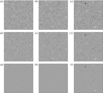
Total vorticity (a–c), vorticity anomaly for
 $\unicode[STIX]{x1D714}_{thr}=\unicode[STIX]{x1D714}_{thr}^{p}=\unicode[STIX]{x1D714}_{rms}$
(d–f), and coherent vorticity (g–i) fields for narrowband hyperviscous (NB4h) simulation at
 $t=2.6,3.7,7.3$
(left to right). The subdomain is
 $384^{2}$
grid points, corresponding to side lengths
 $96l_{f}$
, where
 $l_{f}$
is the forcing length scale.

In this section we study the effect of the forcing Reynolds numbers
 $Re_{f}$
,
 $Re_{d}$
and
 $Re_{\unicode[STIX]{x1D708}}$
on vortex population statistics. We consider a series of simulations with hyperviscosity and narrowband
 $\unicode[STIX]{x1D6FF}$
-correlated forcing at
 $k_{f}=1280,1536,1792,1920$
, 2048, as well as a Markovian simulation with constant forcing at
 $k_{f}=2048$
.
We begin by examining the vorticity fields from the
 $\unicode[STIX]{x1D6FF}$
-correlated simulation with the lowest Reynolds numbers, NB4h, which is forced at
 $k_{f}=2048$
. The forcing wavenumber is very close to both dissipation wavenumbers in this simulation, with
 $k_{d}/k_{f}=1.01$
and
 $k_{\unicode[STIX]{x1D702}}/k_{f}=1.08$
as given in row 7 columns 7–8 of table 1, yielding Reynolds numbers
 $Re_{d}\approx Re_{\unicode[STIX]{x1D708}}\approx 1$
, and
 $Re_{f}=1.5$
. The total vorticity field and the field of high intensity vorticity anomalies, defined by the procedure described in § 4, are shown in figure 12(a–c and g–i, respectively) at times
 $t=2.6,3.7,7.3$
(left to right) on subdomains with side length
 $96l_{f}$
, where
 $l_{f}$
is the forcing length scale. We have set the minimum allowed size
 $A_{min}=\unicode[STIX]{x03C0}r_{min}^{2}$
, with
 $r_{min}=\unicode[STIX]{x03C0}/k_{max}$
, extracting all high-intensity structures at resolvable scales. We have also set the minimum allowed peak vorticity to
 $\unicode[STIX]{x1D714}_{thr}^{p}=2\unicode[STIX]{x1D714}_{rms}$
, noting that the increased effect of dissipation can be expected to suppress vorticity extrema more than at higher Reynolds number. The vorticity field is grainy and lacks the characteristic filamentary structures usually associated with the cascade of enstrophy to small scales. The intense circular coherent vortices that were observed in figure 4 above are also absent at the earlier times
 $t=2.6$
and
 $t=3.7$
, and one might suppose that the lack of enstrophy cascade prevents coherent structures from forming at all at such a low Reynolds number. What is surprising, however, is that even for such low Reynolds numbers like-sign vorticity still aggregates into clusters of same-sign anomalies. This is reminiscent of the aggregation process observed previously in inverse energy cascades without vortices (Tabeling Reference Tabeling2002). To illustrate the aggregation process, in the middle row we show the vorticity anomaly field for a cutoff
 $\unicode[STIX]{x1D714}_{thr}=\unicode[STIX]{x1D714}_{thr}^{p}=\unicode[STIX]{x1D714}_{rms}$
: like-sign anomalies clearly cluster together, providing a formation mechanism for the relatively intense regions visible in the lower left and middle panels of figure 12, although these regions are of weaker intensity, and less circularly symmetric than the strong coherent vortices found at higher Reynolds numbers. By
 $t=7.3$
(when the spectral peak is still well away from the domain scale) more intense circular vortices have formed through clustering and merger of these weaker and less well-defined vortices. Formation of well-defined vortices by aggregation and merger of vorticity anomalies represents a route to coherent vortex formation distinct from the more immediate axisymmetrization of forcing anomalies seen at intermediate Reynolds number, and demonstrates the strong tendency of the inverse cascade in this system to form coherent vortices.
This early flow evolution leading to the emergence of coherent structures resembles that seen in decaying flows started from self-similar Gaussian initial conditions, where patches of vorticity aggregate, in time leading to anelastic collisions between well-defined coherent vortices (Benzi et al.
Reference Benzi, Patarnello and Santangelo1988). The two-point probability density functions (p.d.f.s) shown in figure 13 also illustrate the coherent vortex formation – between
 $t=2.6$
and
 $t=3.7$
there is only a small broadening of the tails, but by
 $t=7.3$
broad tails have formed on all p.d.f.s.
Two-point p.d.f.s of vorticity (a), longitudinal velocity (b) and transverse velocity (c) for simulation NB4h at a separation of
 $32l_{f}$
at
 $t=2.6,3.7,7.3$
, corresponding to the fields shown in figure 12.

Energy flux
 $\unicode[STIX]{x1D6F1}(k)$
(a) and percentage
 $100f_{v}$
(b) of the domain occupied by vortices or high vorticity regions for the indicated simulations.

Having established a robust tendency to form vortices even in the most strongly dissipated member of this set of simulations, we now move on to a more quantitative comparison of the vorticity anomaly fields at various values of the Reynolds number. The energy flux to large scales and the area fraction occupied by vorticity anomalies and coherent vortices are shown in figures 14(a) and 14(b), respectively for the series of experiment NB4d–NB4h with decreasing forcing Reynolds number. As expected, the energy flux to small
 $k$
decreases with decreasing Reynolds number as more energy is dissipated immediately at the scale of the forcing. Comparing the fluxes for NB4h and NB4Mh, which have
 $\unicode[STIX]{x1D6FF}$
-correlated and constant forcing, respectively, it is evident that, all else equal, constant forcing produces a stronger energy flux to large scales.
In analysing the time evolution of the area fraction, it was found necessary to modify the dimensionless time used in the last section. At the lowest Reynolds numbers considered, the evolution of the energy at early times before the inverse cascade is established shows a significant departure from linear growth, resulting in non-constant
 $\unicode[STIX]{x1D700}$
. In these cases, it is therefore more natural to use, in place of
 $t/\unicode[STIX]{x1D70F}_{E}$
, a dimensionless time defined by
 $$\begin{eqnarray}\displaystyle & \displaystyle T_{E}(t)=\int _{0}^{t}[\unicode[STIX]{x1D70F}_{E}(t^{\prime })]^{-1}\,\text{d}t^{\prime }. & \displaystyle\end{eqnarray}$$
Figure 14(b) shows the area fraction occupied by vorticity anomalies and coherent vortices, as identified by the extraction algorithm, plotted against this dimensionless time. Two features are worth noting. First, in the simulations with
 $\unicode[STIX]{x1D6FF}$
-correlated forcing, the area fraction tends to a constant value that exhibits a clear dependence on Reynolds number, with the area fraction decreasing monotonically as Reynolds number decreases. Concurrently the spectrum shallows toward the Kraichnan
 $-5/3$
scaling (figure 15). Plotting the compensated spectrum
 $E(k)k^{5/3}/\unicode[STIX]{x1D700}^{2/3}$
for simulations NB4h and NB4Mh yields a plateau with a Kolmogorov–Kraichnan constant of approximately 7, close to the theoretically predicted value 6.69 (Kraichnan Reference Kraichnan1971). In contrast, there is no clear plateau in the compensated spectrum
 $E(k)k^{5/3}/\unicode[STIX]{x1D700}^{2/3}$
for the simulations with moderate forcing Reynolds number, and the value is generally significantly greater than predicted by Kolmogorov–Kraichnan theory. It should be emphasized that the decrease in coherent area fraction is not a direct consequence of the lower energy input rate at small
 $Re$
: lowering
 $\unicode[STIX]{x1D700}_{I}$
at fixed Reynolds number has no effect on the area fraction. Rather, the decrease in both energy growth and final area fraction are a consequence of decreasing Reynolds number. Second, the case NB4Mh, identical to NB4h but with steady, rather than
 $\unicode[STIX]{x1D6FF}$
-correlated, forcing shows much stronger development of vorticity anomalies (which are not necessarily coherent), despite having a comparable level of energy flux to large scales. The area fraction continues growing with time and does not show the same tendency to level off as in the
 $\unicode[STIX]{x1D6FF}$
-correlated simulations.
Energy spectra (a,b) and local slopes (c,d) averaged over equal intervals in
 $\text{log}(k)$
. Simulations NB4b, NB4d, NB4e, NB4f, NB4g and NB4h (top to bottom spectra in panel a) are shown in (a,c) and the dissipation-range forced simulations NB4h and NB4Mh are shown in (b,d).

(a)
 $A_{max}$
as a function of dimensionless time; the upper and lower solid curves are the similarity predictions
 $\unicode[STIX]{x03C0}(l_{\unicode[STIX]{x1D714}}/2)^{2}$
for simulations NB4d and NB4h respectively. (b)
 $k_{p}$
as a function of dimensionless time; the upper and lower solid lines are the similarity predictions
 $k_{E}=2\unicode[STIX]{x03C0}/l_{E}$
for simulations NB4d and NB4h respectively.

The growth rates of the maximum vortex size,
 $A_{max}$
(a), and the peak of the energy spectrum,
 $k_{p}$
(b), are shown in figure 16. The two heavy black curves are the similarity predictions
 $\unicode[STIX]{x03C0}(l_{\unicode[STIX]{x1D714}}/2)^{2}$
(a) and
 $2\unicode[STIX]{x03C0}/l_{E}$
(b) for simulation NB4d (top curves) and NB4h (bottom curves), the outlying members of the set of simulations. Both the vortex area and the spectral peak wavenumber evolve in accordance with the similarity predictions, and the agreement in magnitude is good. Hence, the characteristic length scales predicted by the similarity arguments show little sensitivity to forcing Reynolds number, demonstrating the wide range of validity of this part of the theory.
Number density
 $n(A/A_{f})$
for the indicated simulations and dimensionless times, with slope lines for comparison.

Finally, the vortex number density is shown in figure 17 for the
 $\unicode[STIX]{x1D6FF}$
-correlated forcing simulations (a) and the lowest Reynolds number
 $\unicode[STIX]{x1D6FF}$
-correlated and constant forcing simulations NB4h and NB4Mh (b). The times chosen in (a) are the latest for which data are available for each case. All
 $\unicode[STIX]{x1D6FF}$
-correlated simulations have a three-part density, approximately following the
 $-3$
,
 $-1$
and
 $-6$
scaling laws found in intermediate forcing Reynolds number simulations. Referring to (b), we note that, remarkably, the three-part number density is obtained even in the simulation NB4h, at a time when there is a complete absence of intense circular vortices, with a short scale-invariant distribution of areas at intermediate scales. We postulate that the aggregation and merger process observed in the vorticity anomaly field, as well as in the coherent vortex population at intermediate Reynolds number, is responsible for the generation of this scaling range. For completeness, in (b) we also illustrate the difference between the number densities for the NB4h with
 $\unicode[STIX]{x1D6FF}$
-correlated forcing and NB4Mh with constant forcing: the latter simulation does not exhibit the scale-invariant
 $-1$
range at intermediate scales at all, but does exhibit the
 $-3$
thermal bath and a steepening at large scales – these ranges thus appear more robust than the scale-invariant intermediate range. The results for NB4Mh are consistent with those for NB4Mb: in both cases the scaling in the intermediate range is spoiled: for dissipation-range forcing the range does not exist at all, while for intermediate forcing it is steeper than expected.
7 Conclusions
We have studied the sensitivity to simulation parameters of the similarity and vortex scaling theories for the inverse energy cascade developed by Burgess & Scott (Reference Burgess and Scott2017). We varied forcing bandwidth, forcing correlation time, choice of dissipation operator and Reynolds number. The similarity arguments accurately predict the evolution of the spectral peak and the largest vortex area in all simulations, demonstrating the wide validity of these arguments based on globally integrated quantities, energy and enstrophy. The vortex scaling ranges are largely insensitive to forcing bandwidth and the dissipation operator. The vortex intensity
 $\overline{\unicode[STIX]{x1D714}_{v}^{2}}$
grows in all hyperviscous simulations, but not in the Laplacian simulations, showing that – in contrast to the number of scaling ranges and their slopes – the time evolution of the vortex intensity is not robust to choice of dissipation.
The dependence on forcing Reynolds number showed some interesting features. In particular, for white-in-time forcing, even the simulation with the lowest forcing Reynolds number, in which the enstrophy cascade is absent and in which the vorticity anomaly field consists of comparatively amorphous regions, develops a three-part number density with approximately the predicted scaling ranges. Vorticity anomalies in this simulation aggregate and merge, forming larger structures, eventually culminating in the formation of intense circular vortices at late times. Based on this observation, we hypothesize that the process of aggregation and merger generates the intermediate scale-invariant
 $A^{-1}$
range, which can thus arise for both amorphous vorticity anomalies and well-defined circular coherent vortices, as long as the aggregation process is not particularly sensitive to the spatial profile of the vorticity anomalies.
The greatest differences in the vortex number density arise in comparing simulations with constant forcing to those with
 $\unicode[STIX]{x1D6FF}$
-correlated forcing: at high enough values of viscosity, the intermediate scale-invariant range steepens significantly past the predicted
 $A^{-1}$
slope in the flows with constant forcing; relatedly, there is a shorter thermal bath and a more gradual transition to the large-scale steep range. We speculate that the steepening of the intermediate range may be due to correlations between the streamfunction and forcing, which were found to increase with dissipation. Since large-scale streamfunction regions are associated with clustering of anomalously intense vorticity regions, and since such clustering might be expected to affect details of scale invariance, it seems reasonable that changes in the statistics of the streamfunction would affect the aggregation process and disrupt the scale-invariant intermediate range. We will study this issue and the spatial characteristics of the vortex populations in the three scaling ranges in more detail in future work.
Acknowledgements
Simulations were run on the St Andrews MHD Cluster. B.H.B. is supported by a Leverhulme Early Career Fellowship from the Leverhulme Trust. The Natural Environment Research Council grant NE/M014983/1 also supported B.H.B. while this work was completed.